Outdoor Air Temperature Measurement: A Semi-Empirical Model to Characterize Shelter Performance

 , , , and
Abstract
:1. Introduction
1.1. Context
1.2. Air Temperature Error Estimation
- Data analysis of in situ and laboratory measurement campaigns,
- Empirical modeling from observations,
- Physical modeling.
1.2.1. Data Analysis of In Situ and Laboratory Measurement Campaigns
1.2.2. Empirical Modeling from Observation
- is the air temperature error due to a shield at time t
- is the regression coefficient attributed to the term
- is the value of an explanatory variable
- and are calculated using regression fitting
- = 1.2 kg·m the mass density of the air
- = 1004 J·K·kg the specific heat capacity of the air
- the zenithal solar angle (in degree)
1.2.3. Physical Modeling
1.3. Objective of the Study
- To propose a transfer function that highlights the two main characteristics of a shield: radiation sensitivity and temperature response time
- To verify the physical relevance of the proposed model using the observations
- To evaluate the model ability to accurately estimate the shield induced temperature error.
2. Material and Methods
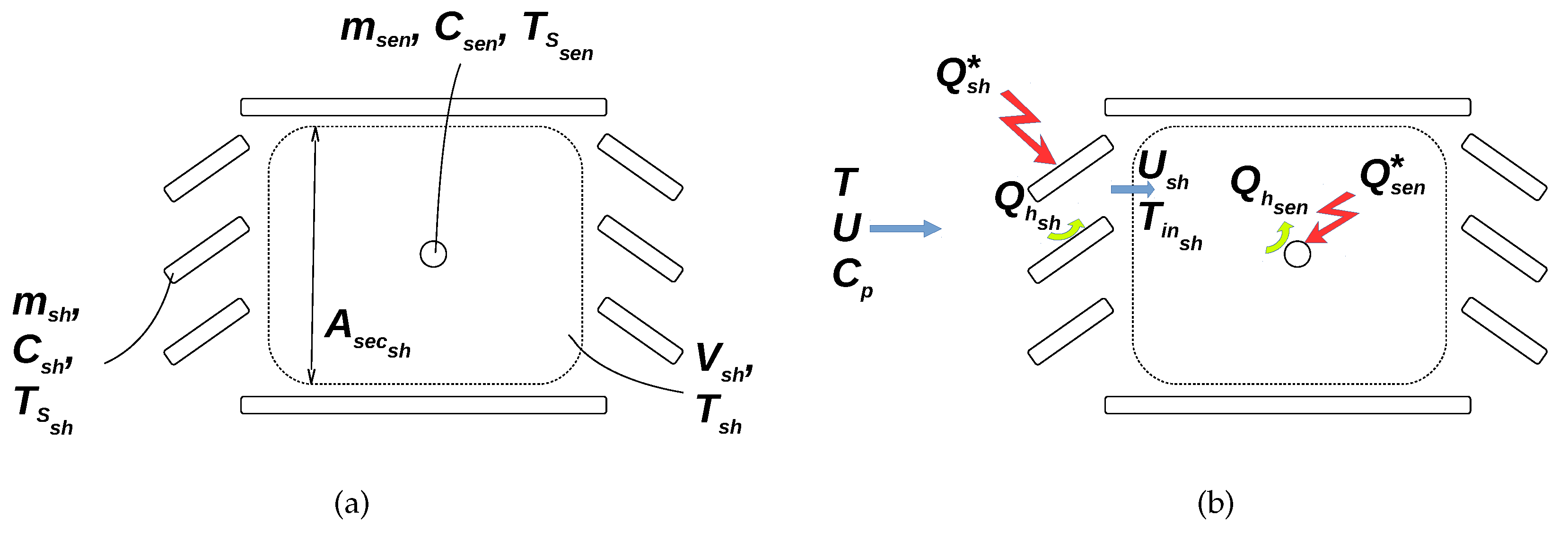
2.1. Proposed Shelter Physical Model
- the shelter weight (kg)
- the specific heat of the shelter (J·kg·K)
- the time derivative of the shelter surface temperature (K·s)
- the shelter surface (m2)
- the shelter net global radiation density (W·m)
- the shelter convective heat flux density (W·m)
- the surface of the vertical shelter cross-section (m2)
- the vertical averaged wind speed inside the shelter (m·s)
- the volume-specific heat of the air (J·m·K)
- the temperature of the air entering within the shelter (K)
- T the outside air temperature (K)
- the ratio of the shelter convective heat flux density which is transported within the shelter
- the sensor weight (kg)
- the specific heat of the sensor (J·kg·K)
- the volume of air included within the shelter (m3)
- the time derivative of the temperature of the system {sensor + air contained within the shelter} (K·s)
- the sensor surface (m2)
- the sensor net global radiation density (W·m)
- t the time (s)
- (m)
- (m2·K·J)
- (m2·K·J)
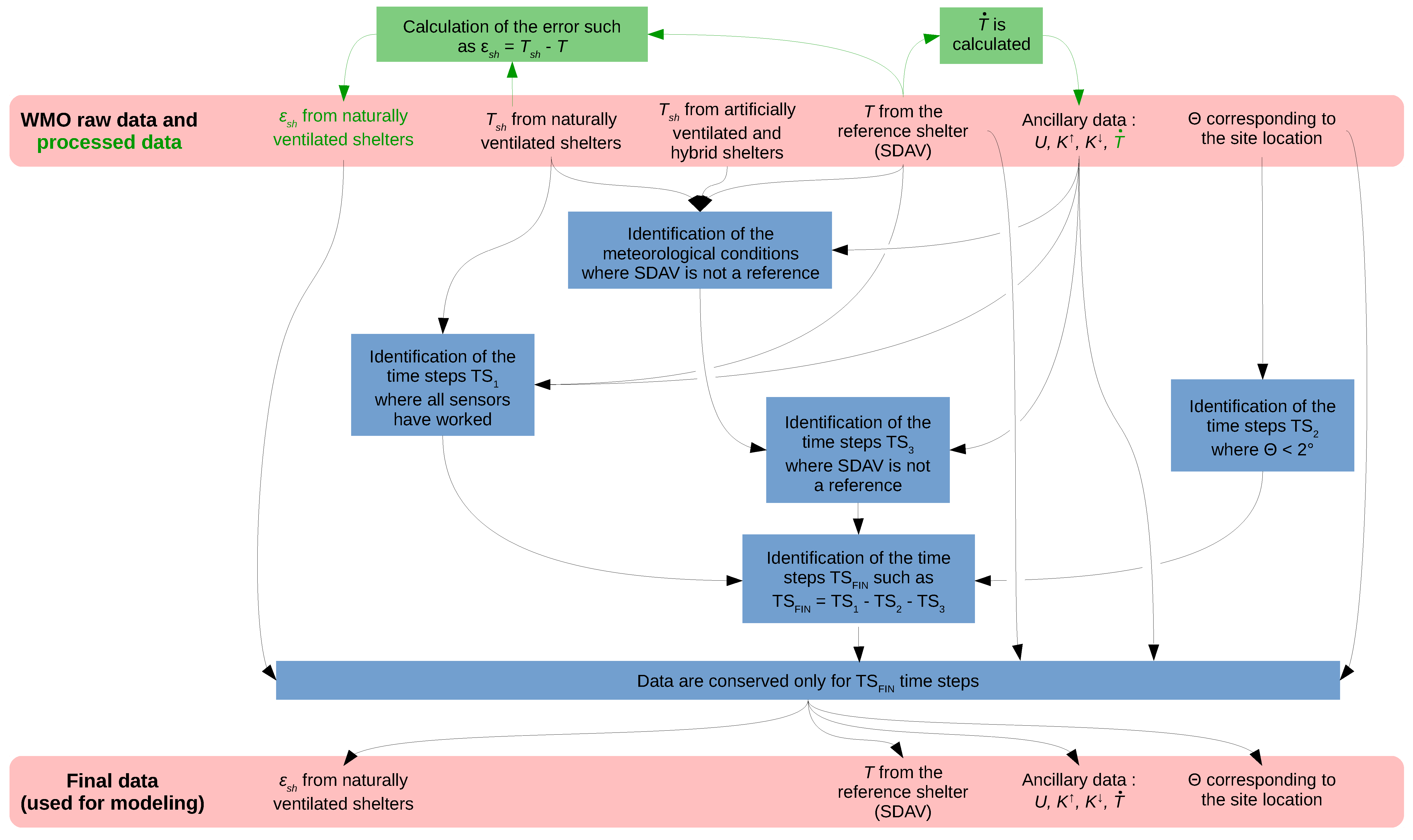
2.2. Data
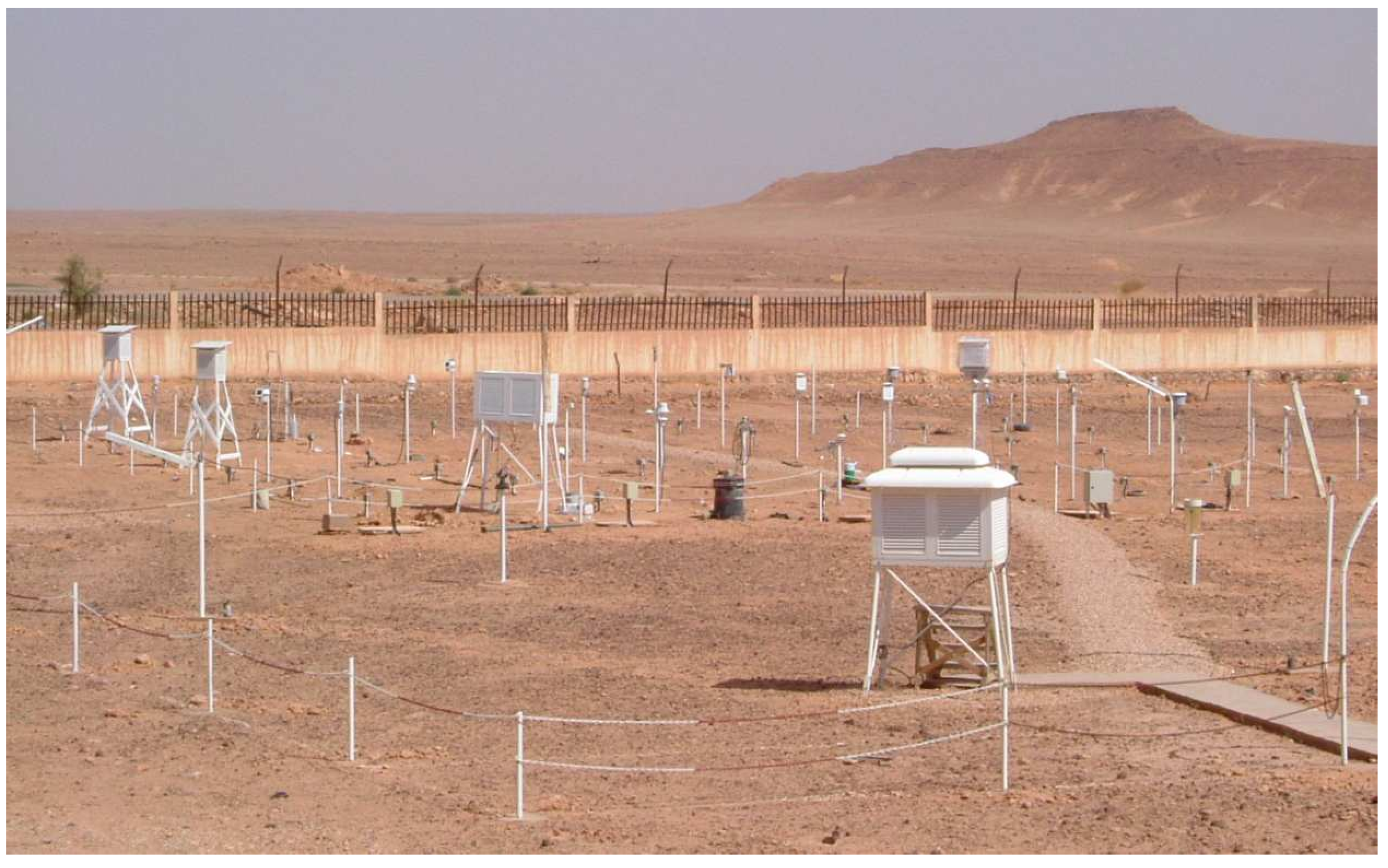
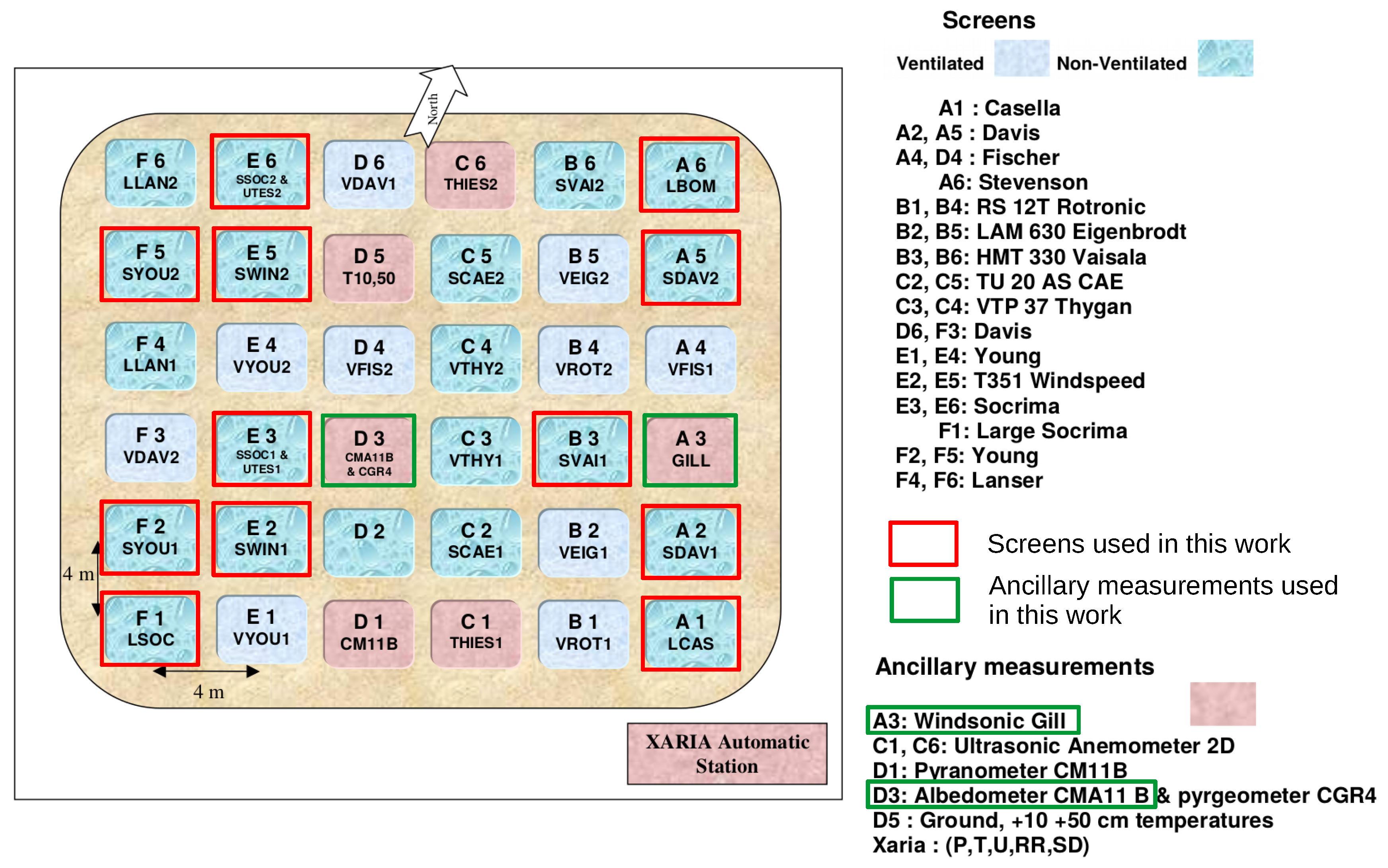
2.2.1. Location
2.2.2. Measurement of the Air Temperature within the Shields
2.2.3. Compatibility between the Observed Meteorological Variables and the Model Terms
- It should follow the outside air temperature as quickly as possible.
- It should be the least sensible to global radiation. According to the ISO17714:2007 standard, screens “that are cooler during the day and warmer during the night are likely to be giving measurements that are closest to the truth” [13].
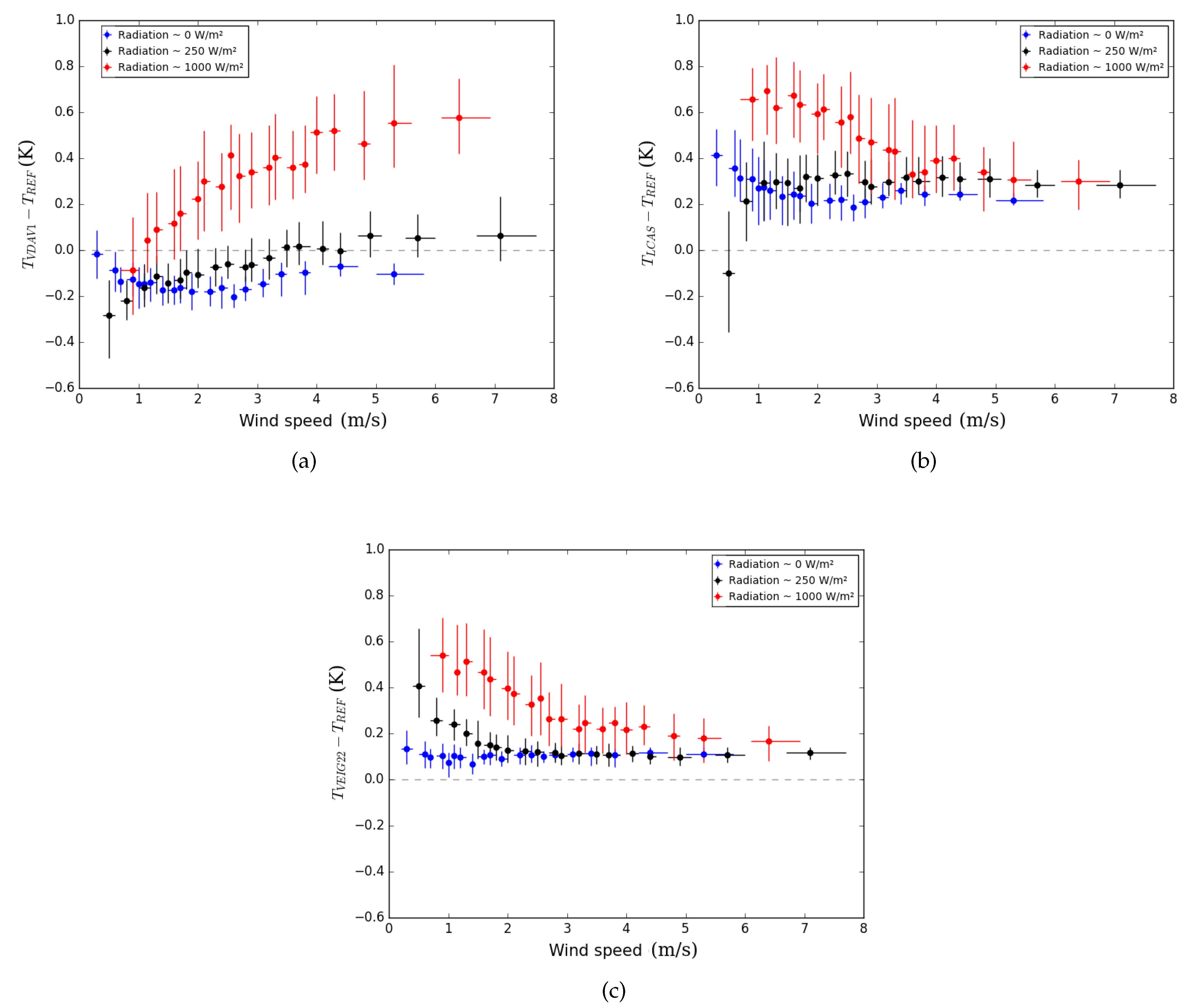
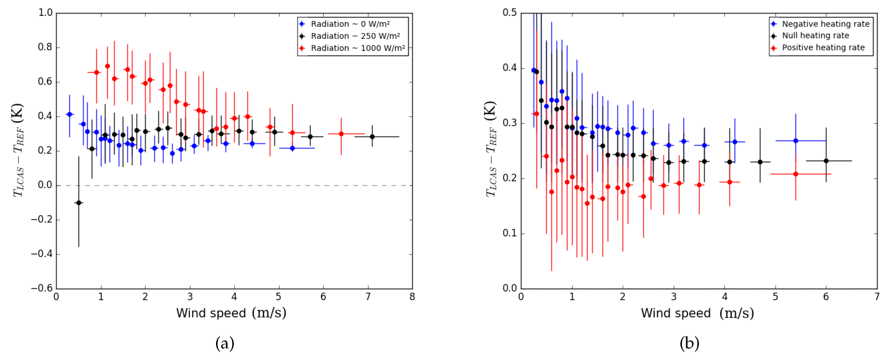
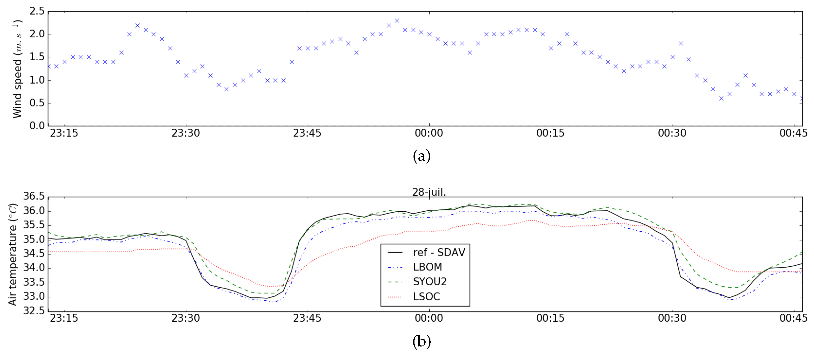
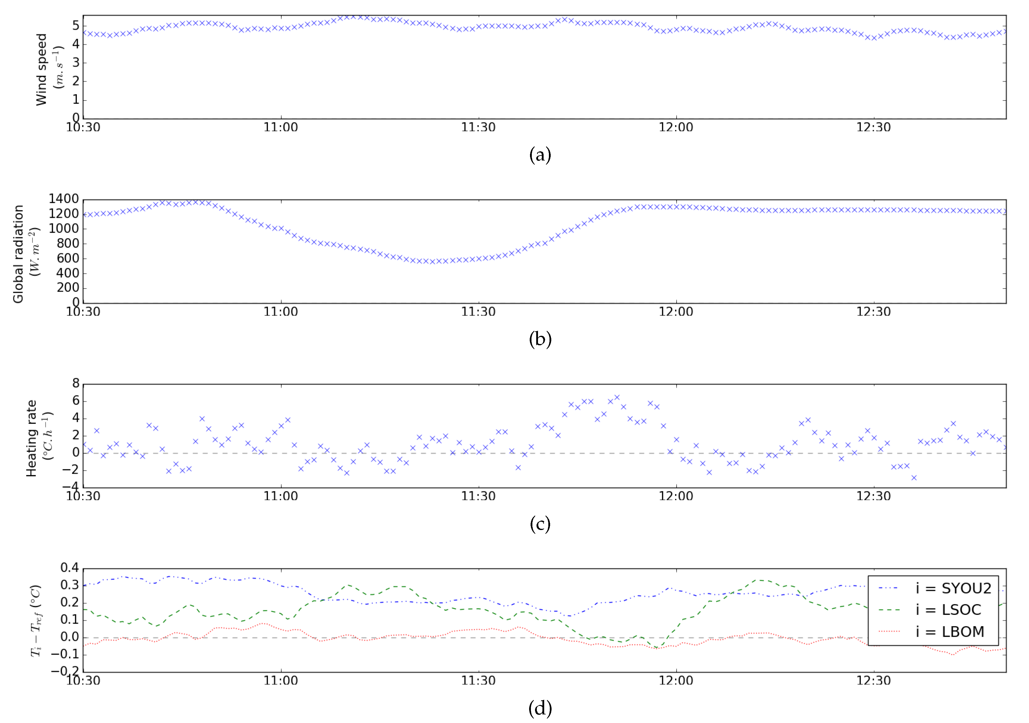
- Under wind speed lower than 1 m·s and whatever the radiation, SDAV temperature is not the highest during night-time neither the lowest during day-time (Figure 4a)
- Under low wind speed and low solar height (about 30 for the 250 W·m radiation curve), SDAV is more impacted by the radiation than some other naturally ventilated shelters (Figure 4b)
- When the wind speed increases, every hybrid or naturally ventilated shelter temperature tends toward a different value whereas they were expected to tend toward SDAV temperature (Figure 4b,c).
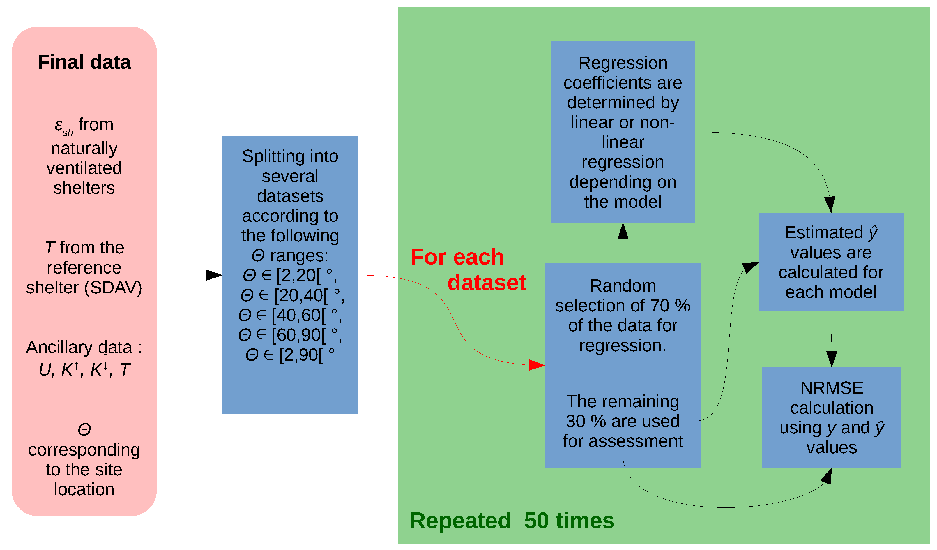
2.3. Model Regression
- y is estimated according to the observed y at the previous time step: this case is an ideal case,
- y is estimated according to the estimated y of the previous time step, itself estimated using the estimated y of the previous time step, etc. The number of previous time steps taken into account for the estimation of the error might be a critical parameter affecting the model performance. Thus, several values have been tested: 0, 5, 10, 15, 20, 25, and 30 time steps.
- (%) the normalized RMSE of the shelter when its data have been corrected by a given model
- (C) the RMSE of the shelter when its data have been corrected by a given model
- (C) the RMSE of the shelter when its data have not been corrected (raw data)
- N the number of time steps used for the calculation
- the air temperature error observed within shelter
- the air temperature error estimated within shelter according to a given model
3. Results
3.1. Physical Relevance of the Proposed Model
3.1.1. Explanatory Variables
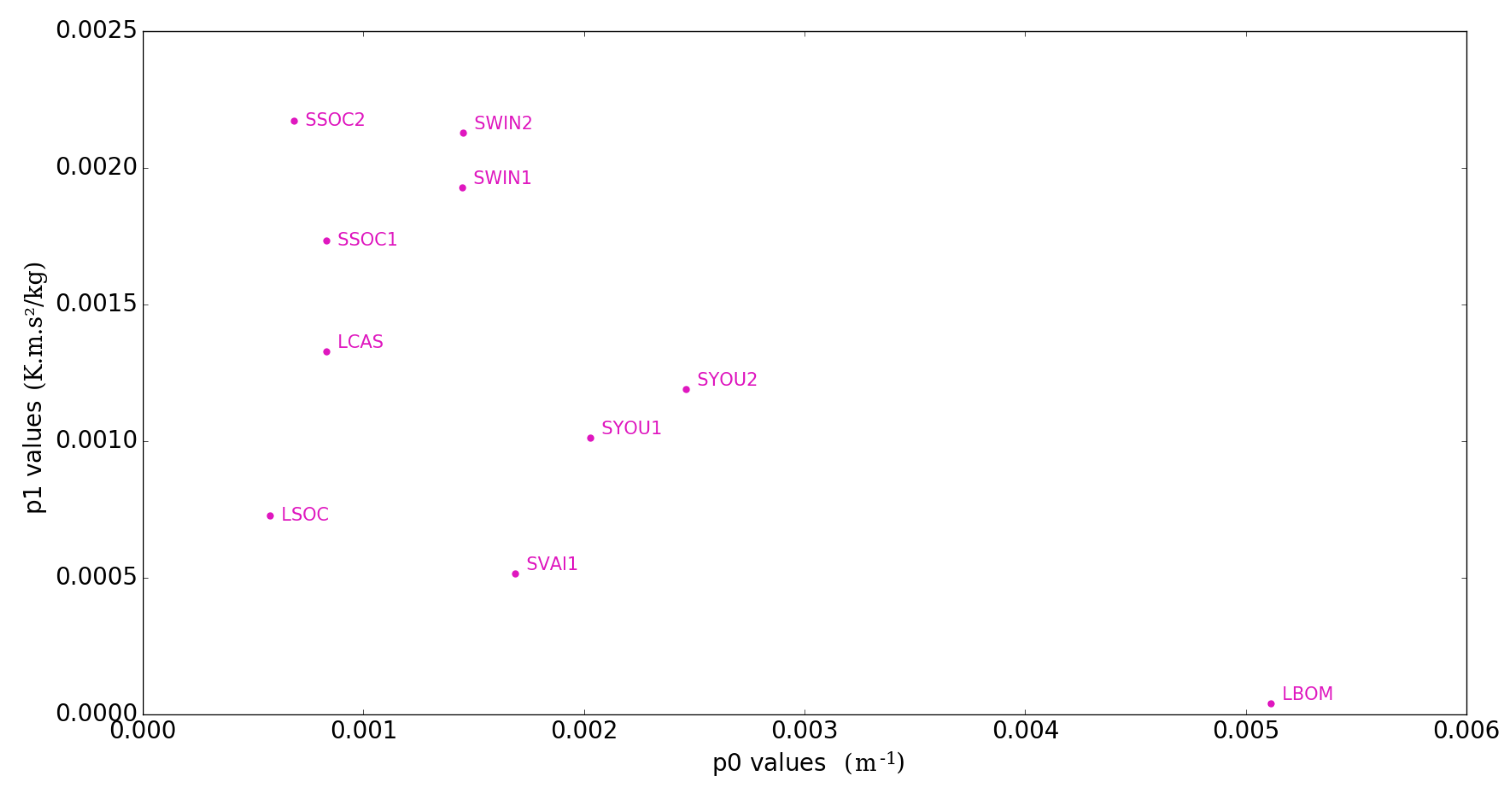
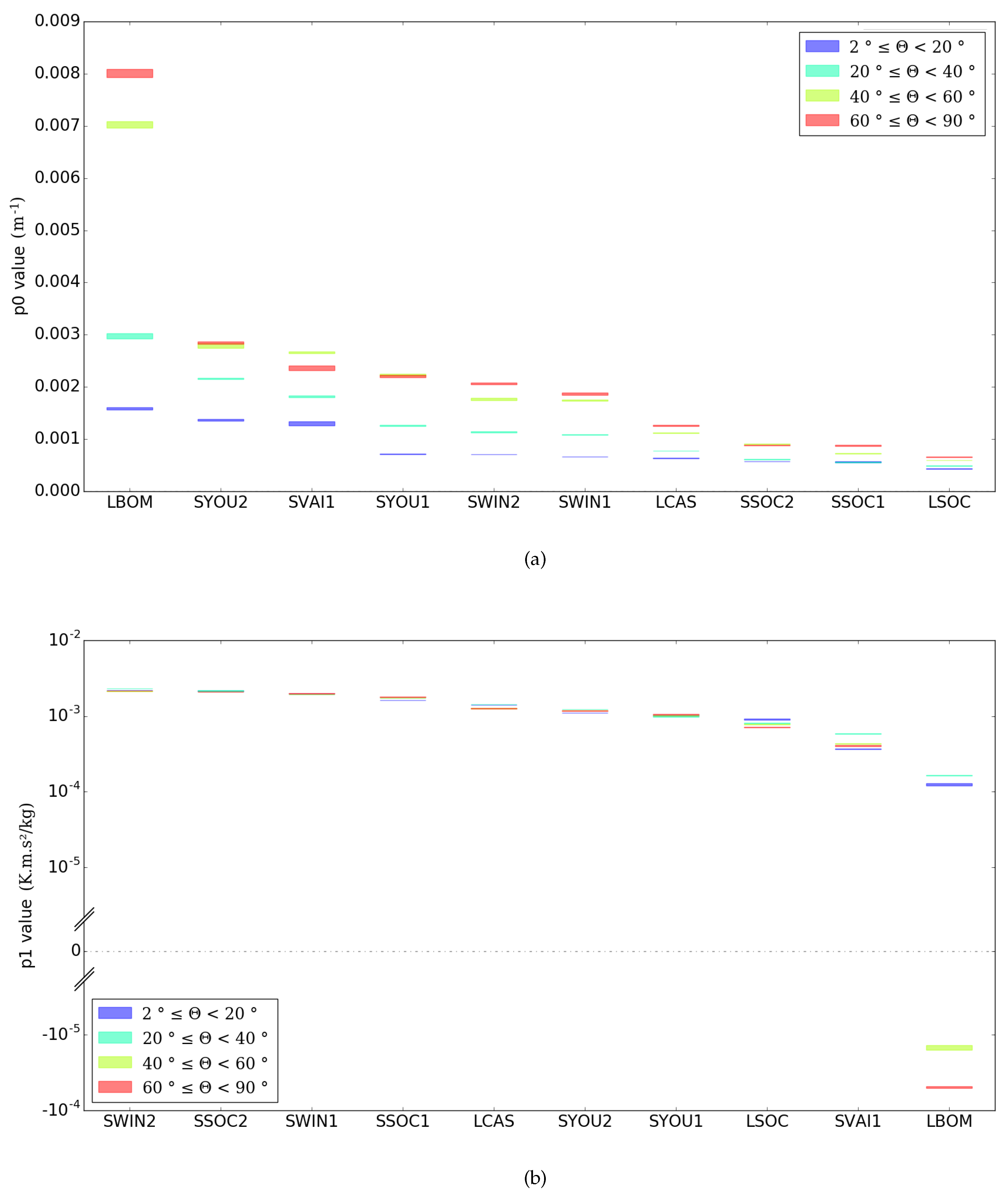
3.1.2. Regression Coefficients
- is the time constant of the shelter
- the regression coefficient value for shelter
3.1.3. Sensitivity Regarding the Solar Azimuth Angle
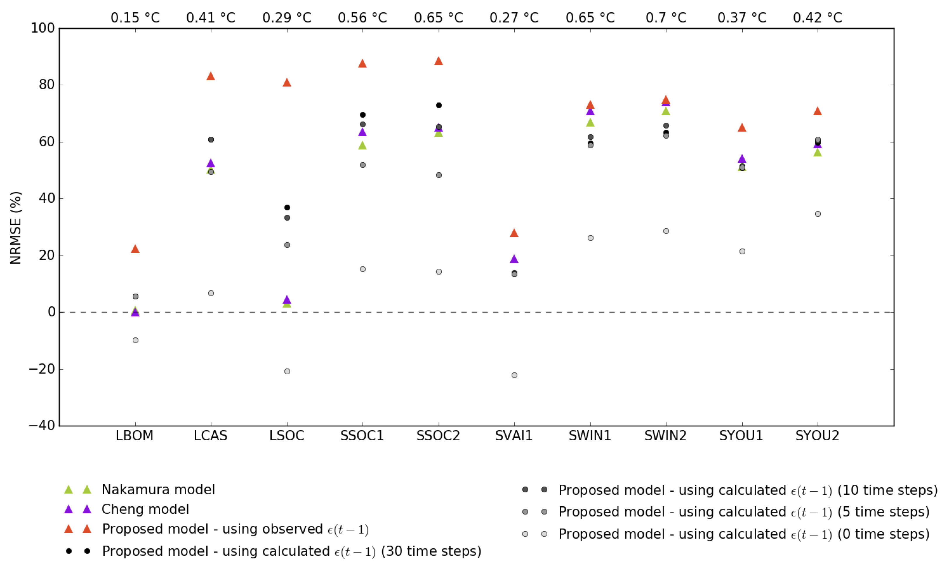
3.2. Comparison of the Models Performance
4. Discussions
- The response time is attributed to the shelter ventilation rate. The regression coefficient related to this phenomenon showed consistency with observation. However, this is contradictory with Lin et al. [6] observations showing that the horizontal wind speed along the central vertical axis of a shelter was sufficiently high to assume an almost instantaneous air renewal.
- To obtain our semi-empirical model, the sensor and the air within the shelter were considered as having the same temperature at any time, which is contradictory with Erell et al. [11], de Podesta et al. [5] findings. However, the results obtained using this model are consistent with the observation.
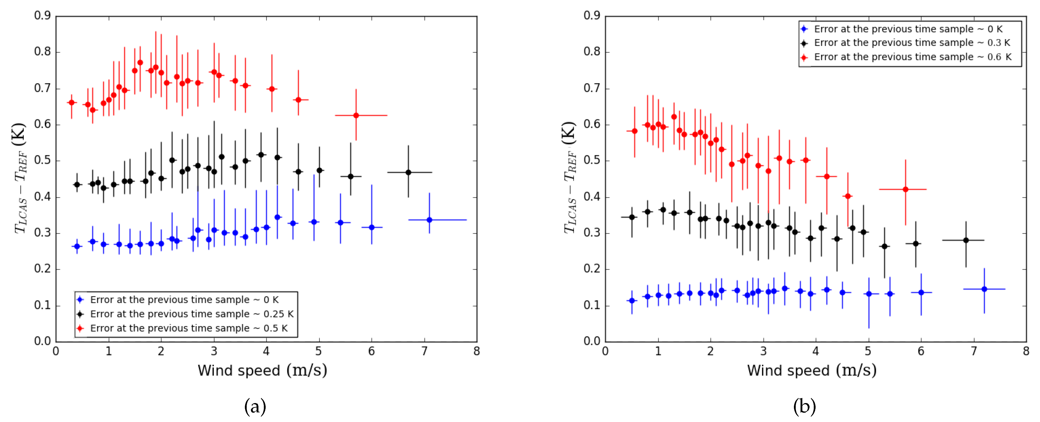
- The error does not tend toward zero when the wind speed increases. The offset seems to be directly dependent on the heating rate value.
- The three models compared in this study could be calibrated using only variables commonly measured on meteorological sites (descending solar radiation, wind speed, and air temperature). The objective would then be to evaluate their respective ability to estimate the error observed at several other locations.
- Hybrid and artificially ventilated shelters have not been modeled while it is fundamental to compare their characteristics (response time and sensitivity to radiation) to naturally ventilated shelters.
- The long-wave radiation was not used in this study. A measurement campaign where this meteorological variable is available would be welcome to further evaluate the model and verify its performances during night-time.
- The shelter used for the reference temperature is far from being perfect. Lanzinger and Langmack [15] proposed a calibration method in climatic chamber to access air temperature from an ultrasonic anemometer but as pointed by Richiardone et al. [16], further work should be done to obtain error-less air temperature from acoustic thermometric.
Author Contributions
Funding
Acknowledgments
Conflicts of Interest
Abbreviations
| WMO | World Meteorological Organization |
| RMSE | Root Mean Square Error |
Appendix A. Detailed Informations about the WMO Shelters and Their Respective Performances

| Acronym | Manufacturer | Type | Ventilation Type | Closest Shape | Material | Number of Shelters |
|---|---|---|---|---|---|---|
| LBOM | BoM | Small Stevenson screen | natural | cuboid | wood | 1 |
| LCAS | Casella | Stevenson screen | natural | cuboid | wood | 1 |
| LLAN | Lanser | hybrid | cuboid | wood | 2 | |
| LSOC | Socrima | Large Stevenson screen | natural | cuboid | plastic | 1 |
| SCAE | CAE | TU20AS | natural | cylindric | duralinium | 2 |
| SDAV | Davis | PN7714 | natural | cuboid | plastic | 2 |
| SSOC | Socrima | BMO1195D | natural | cylindric | plastic & steel | 2 |
| SVAI | Vaisala | DTR13 (HMT 330 MIK) | natural | cylindric | polyester & fiberglass | 2 |
| SWIN | Windspeed | T351-PX-D/3 | natural | cylindric | ABS & aluminum & nylon | 2 |
| SYOU | Young | 41003 | natural | cylindric | Thermoplastic & steel & aluminum | 2 |
| VDAV | Davis | 07755 | artificial | cylindric | plastic | 2 |
| VEIG | Eigenbrodt | LAM630 | hybrid | cylindric | ABS synthetic & acryl glass | 2 |
| VFIS | Fisher | 431411 | artificial | cylindric | aluminum | 2 |
| VROT | Rotronic | AG/RS12T | artificial | cylindric | aluminum | 2 |
| VTHY | Meteolabor | Thygan VTP37 Airport & Thygan VTP37 Thermohygrometer | artificial | cuboid | aluminum | 2 |
| VYOU | Young | 43502 | artificial | cylindric | Thermoplastic & steel & aluminum | 2 |
| Screen Type | Screen Acronym | Screen i Is Equal or Better than ref | Screen i Worse than ref | ||||
|---|---|---|---|---|---|---|---|
| Under Low G Values | Under Medium G Values | Under High G Values | Insensible to Wind Speed for Low G Values | When , K for Any G Value | Increases with Wind Speed | ||
| Natural ventilation | LBOM | when m·s | when m·s and m·s | for any wind speed | |||
| LCAS | when U < 1 m·s | when m·s | K | ||||
| LSOC | when m·s | when m·s and m·s | when m·s | K | |||
| SSOC1 | K | K | |||||
| SSOC2 | K | K | |||||
| SVAI1 | for any wind conditions | for any wind conditions | for any wind conditions | ||||
| SWIN1 | K | ||||||
| SWIN2 | K | ||||||
| SYOU1 | when m·s | K | |||||
| SYOU2 | when m·s | K | |||||
| Artificial ventilation | LLAN1 | when m·s | K | ||||
| LLAN2 | when m·s | K | |||||
| VEIG11 | for any conditions | when m·s | |||||
| VEIG12 | for any conditions | when m·s | K | ||||
| VEIG21 | when m·s | when m·s | K | ||||
| VEIG22 | when m·s | when m·s | |||||
| Hybrid ventilation | VDAV1 | when m·s | when m·s | when | |||
| VDAV2 | when m·s | when m·s | when | ||||
| VFIS2 | |||||||
| VFIS1 | |||||||
| VROT1 | when m·s | when m·s | when | ||||
References
- Jarraud, M. Guide to Meteorological Instruments and Methods of Observation (WMO-No. 8); World Meteorological Organisation: Geneva, Switzerland, 2008. [Google Scholar]
- Van der Meulen, J. A Thermometer Screen Intercomparison; World Meteorological Organisation: Geneva, Switzerland, 1998; p. 319. [Google Scholar]
- Van der Meulen, J.; Brandsma, T. Thermometer screen intercomparison in De Bilt (The Netherlands), Part I: Understanding the weather-dependent temperature differences. Int. J. Clim. 2008, 28, 371–387. [Google Scholar] [CrossRef]
- Barnett, A.; Hatton, D. Recent Changes in Thermometer Design and Their Impact; World Meteorological Organisation: Geneva, Switzerland, 1998. [Google Scholar]
- Erell, E.; Leal, V.; Maldonado, E. Measurement of air temperature in the presence of a large radiant flux: An assessment of passively ventilated thermometer screens. Bound. Layer Meteorol. 2005, 114, 205–231. [Google Scholar] [CrossRef]
- Lin, X.; Hubbard, K.G.; Meyer, G.E. Airflow characteristics of commonly used temperature radiation shields. J. Atmos. Ocean. Technol. 2001, 18, 329–339. [Google Scholar] [CrossRef]
- Nakamura, R.; Mahrt, L. Air temperature measurement errors in naturally ventilated radiation shields. J. Atmos. Ocean. Technol. 2005, 22, 1046–1058. [Google Scholar] [CrossRef]
- Cheng, X.; Su, D.; Li, D.; Chen, L.; Xu, W.; Yang, M.; Li, Y.; Yue, Z.; Wang, Z. An improved method for correction of air temperature measured using different radiation shields. Adv. Atmos. Sci. 2014, 31, 1460–1468. [Google Scholar] [CrossRef]
- Lin, X.; Hubbard, K.; Walter-Shea, E.; Brandle, J.; Meyer, G. Some perspectives on recent in situ air temperature observations: Modeling the microclimate inside the radiation shields. J. Atmos. Ocean. Technol. 2001, 18, 1470–1484. [Google Scholar] [CrossRef]
- Lacombe, M.; Bousri, D.; Leroy, M.; Mezred, M. WMO Field Intercomparison of Thermometer Screens/Shields and Humidity Measuring Instruments, Ghardaia, Algeria, November 2008–October 2009; World Meteorological Organisation: Geneva, Switzerland, 2011. [Google Scholar]
- De Podesta, M.; Bell, S.; Underwood, R. Air temperature sensors: Dependence of radiative errors on sensor diameter in precision metrology and meteorology. Metrologia 2018, 55, 229. [Google Scholar] [CrossRef]
- Coppa, G.; Garcia Izquierdo, C.; Jandric, N.; Quarello, A.; Voldan, M.; Merlone, A. Experimental evaluation of temperature uncertainty components due to siting conditions with respect to WMO classification. In Proceedings of the EMS Annual Meeting—European Conference for Applied Meteorology and Climatology 2017, Dublin, Ireland, 4–8 September 2017. [Google Scholar]
- ISO. Meteorology—Air Temperature Measurements—Test Methods for Comparing the Performance of Thermometer Shields/Screens and Defining Important Characteristics; World Meteorological Organisation: Geneva, Switzerland, 2007. [Google Scholar]
- Lacombe, M. Results of the WMO intercomparison of thermometer screens/shields and hygrometers in hot desert conditions. In Proceedings of the TECO-2010—WMO Technical Conference on Meteorological and Environmental Instruments and Methods of Observation, Helsinki, Finland, 30 August–1 September 2010. [Google Scholar]
- Lanzinger, E.; Langmack, H. Measuring air temperature by using an ultrasonic anemometer. In Technical Conference on Meteorological and Environmental Instruments and Methods of Observation (TECO-2005), WMO Tech. Doc; World Meteorological Organisation: Geneva, Switzerland, 2005. [Google Scholar]
- Richiardone, R.; Manfrin, M.; Ferrarese, S.; Francone, C.; Fernicola, V.; Gavioso, R.M.; Mortarini, L. Influence of the sonic anemometer temperature calibration on turbulent heat-flux measurements. Bound. Layer Meteorol. 2012, 142, 425–442. [Google Scholar] [CrossRef]


| Size and Orientation of Shield Openings | Shield Albedo & Emissivity | Thermal Characteristics of the Shield Structure (Resistance, Admittance) | |
|---|---|---|---|
| Direct radiation | X | X | |
| Indirect radiation | X | X | |
| Poor shield ventilation | X | ||
| Enthalpy of phase change (water and snow on the shelter) | X |
| Acronym | Manufacturer | Type | Number of Shelters | Location in Figure 3 | Estimated Volume (dm3) | Estimated Section (dm2) | Estimated Surface (dm2) |
|---|---|---|---|---|---|---|---|
| LBOM | BoM | Small Stevenson screen | 1 | A6 | 180 | 36 | 200 |
| LCAS | Casella | Stevenson screen | 1 | A1 | 510 | 64 | 380 |
| LSOC | Socrima | Large Stevenson screen | 1 | F1 | 1000 | 100 | 620 |
| SCAE | CAE | TU20AS (Cylindric multiplate) | 2 | C2, C5 | 17 | 7.8 | 20 |
| SDAV | Davis | PN7714 (Cuboid multiplate) | 2 | A2, A5 | 5.6 | 2.9 | 19 |
| SSOC | Socrima | BMO1195D (Cylindric multiplate) | 2 | E3, E6 | 16 | 10 | 16 |
| SVAI | Vaisala | DTR13-HMT 330 MIK (Cylindric multiplate) | 2 | B3, B6 | 11 | 6.6 | 14 |
| SWIN | Windspeed | T351-PX-D/3 (Cylindric multiplate) | 2 | E2, E5 | 0.50 | 0.80 | 1.8 |
| SYOU | Young | 41003 (Cylindric multiplate) | 2 | F2, F5 | 5.0 | 3.6 | 8.7 |
| Original Needed Variable (Equation (12)) | Substitution Variable (Measured during the WMO Campaign) | Modification Brought Equation (12) | ||
|---|---|---|---|---|
| Sensor Name | Variable Name | Sampling Conditions | ||
| Wind Sonic Gill (Gill) | outside wind speed U | The measurement is performed twice per second. Then a 2 min period moving-average (vectorial) is performed and only the 1 min data is recorded. * | where is a coefficient proper to each shelter | |
| Albedometer CMA11B (Kipp & Zonen) | Ascending and descending short-wave radiation ( and ) | The measurement is performed once every ten seconds. Then an average of the last minute is recorded every 1 min. * | where is the shelter albedo is the solar zenith angle | |
| where is a coefficient proper to each shelter | ||||
| PT100 temperature sensor located within the Davis PN7714 shelter | Outside air temperature T | The measurement is performed once every ten seconds. Then an average of the last minute is recorded every 1 min. * | where and n are two consecutive samples the sampling period T the outside air temperature | |
| Year | 2008 | 2008 | 2009 | 2009 | 2009 | 2009 | 2009 | 2009 | 2009 | 2009 | 2009 | 2009 |
|---|---|---|---|---|---|---|---|---|---|---|---|---|
| Month | 11 | 12 | 01 | 02 | 03 | 04 | 05 | 06 | 07 | 08 | 09 | 10 |
| Time step distribution (%) | 10 | 7.9 | 6.1 | 5.7 | 6.2 | 6.9 | 7.6 | 6.1 | 13.4 | 12.3 | 7.5 | 10.2 |
| Model Name | Model Function | Explanatory Variables | Regression Coefficients |
|---|---|---|---|
| Nakamura | , | ||
| Cheng | , | ||
| Our model | , , , | , |
© 2019 by the authors. Licensee MDPI, Basel, Switzerland. This article is an open access article distributed under the terms and conditions of the Creative Commons Attribution (CC BY) license (http://creativecommons.org/licenses/by/4.0/).
Share and Cite
Bernard, J.; Kéravec, P.; Morille, B.; Bocher, E.; Musy, M.; Calmet, I. Outdoor Air Temperature Measurement: A Semi-Empirical Model to Characterize Shelter Performance. Climate 2019, 7, 26. https://0-doi-org.brum.beds.ac.uk/10.3390/cli7020026
Bernard J, Kéravec P, Morille B, Bocher E, Musy M, Calmet I. Outdoor Air Temperature Measurement: A Semi-Empirical Model to Characterize Shelter Performance. Climate. 2019; 7(2):26. https://0-doi-org.brum.beds.ac.uk/10.3390/cli7020026
Chicago/Turabian StyleBernard, Jérémy, Pascal Kéravec, Benjamin Morille, Erwan Bocher, Marjorie Musy, and Isabelle Calmet. 2019. "Outdoor Air Temperature Measurement: A Semi-Empirical Model to Characterize Shelter Performance" Climate 7, no. 2: 26. https://0-doi-org.brum.beds.ac.uk/10.3390/cli7020026