A Case Study of Ozone Diurnal Variation in the Convective Boundary Layer in the Southeastern United States Using Multiple Observations and Large-Eddy Simulation

Abstract

We investigated the diurnal ozone variation on 6 September 2013 in a midsize urban environment using multiple in situ and remote-sensing measurements along with the Dutch atmospheric large-eddy simulation (DALES) model coupled with a chemical module and a dry deposition module that we added for this study. Our study area was Huntsville, Alabama, USA, a typical midsize city in the Southeastern United States. The ozone variation in the convective boundary layer (CBL) resulted mainly from local emissions and photochemical production stemming from weather conditions controlled by an anticyclonic system on that day. Local chemical production contributes approximately two thirds of the ozone enhancement in the CBL and, in this case, dynamical processes including ozone transport from the free troposphere (FT) to the CBL through the entrainment processes contributed the remainder. The numerical experiments performed by the large-eddy simulation (LES) model showed acceptable agreement with the TOLNet (The tropospheric ozone lidar network)/RO₃QET (Rocket-city ozone quality evaluation in the troposphere) ozone DIAL (differential absorption lidar) observations. This study indicated the need for fine-scale, three-dimensional ozone observations with high temporal and spatial resolution for air quality studies at the urban scale and smaller.

1. Introduction

Ozone is one of the most important air pollutants due to its harmful effects on human health, agriculture, and forests, and the material damage it causes [1,2]. Generally, ozone variations in the convective boundary layer (CBL) are associated with factors such as surface emission and deposition, interaction with the free troposphere (FT), and transport, in addition to the chemical production of NO_x (=NO + NO₂) volatile organic compounds (VOCs) in the presence of sunlight [3,4,5,6,7,8]. In the Southeastern United States, ozone concentrations are more sensitive to nitrogen oxides in rural areas due to the high VOC emissions of dense forests [9,10]. In urban areas (e.g., Atlanta, Georgia, USA), ozone concentrations are sensitive to both nitrogen oxidants and VOCs from both anthropogenic and natural sources [9,11]. Additionally, air stagnation regimes have more influence on the episode days than synoptic-scale transport in the Southeastern United States [12]. Ground ozone variation at small and urban scales is receiving increasing attention due to the dramatically growing population in urban areas [13,14,15,16,17]. Urbanization processes can influence a wide range of the atmospheric flow, including the surface–air exchange, turbulence regime, micro–climate, and, accordingly, can change the transport, dispersion, and deposition of atmospheric pollutants including ozone. The National Aeronautics and Space Administration (NASA) plans to launch a geostationary air quality satellite, tropospheric emissions: monitoring of pollution (TEMPO), providing high spatiotemporal observations [18,19]. Furthermore, air quality studies with fine scales are one of the most important foci in recent field campaigns (e.g., DISCOVER–AQ—deriving information on surface conditions from column and vertically resolved observations relevant to air quality, and SEAC⁴RS—studies of emissions and atmospheric composition, clouds and climate coupling by regional surveys) [20,21,22].

Thorough knowledge of urban CBL structure is the key to understanding satellite observations and forecast modeling of fine-scale air quality studies. However, studies of urban CBL structures are very challenging due to factors such as the paucity of fine resolution observations, emission and deposition inventories, and the coarse resolution of current air quality models [13,15,23,24]. Several studies have utilized, with considerable success, lidar measurements and large-eddy simulation (LES) models to study air quality with fine resolution by taking advantage of the strengths of observations and simulations with fine resolution [3,25,26,27,28,29]. In this research, we combined the strengths of the lidar and LES models for fine-scale urban air quality studies to investigate the impacts of the CBL chemical and dynamical processes on diurnal ozone variation in Huntsville, Alabama, a typical midsize city in the Southeastern United States.

The subsequent structure of this paper is as follows: Section 2 describes the measurements, model and methodology, Section 3 provides a discussion and analysis of the results, and Section 4 summarizes and concludes this study.

2. Measurements and Model

2.1. Measurements

Observations were collected on 6 September 2013 during the SEAC⁴RS field campaign, which included ozone and meteorological fields from multiple platform instruments located on the campus of the University of Alabama in Huntsville (UAH 34.724°N, 86.645°W) [3,30]. Local standard time in Huntsville, Alabama (USA central time zone) is 5 h earlier (GMT-5) according to the universal time coordinate (UTC).

The tropospheric ozone lidar network (TOLNet) Rocket-city ozone quality evaluation in the tropospher (RO₃QET) differential absorption lidar (DIAL) was developed jointly by the University of Alabama in Huntsville (UAH) and the NASA Goddard Space Flight Center (GSFC). This DIAL consists of two 30 Hz Nd:YAG-pumped Raman-shifted lasers at 289 and 299 nm, respectively, and three receivers (2.5, 10, and 40 cm) to cover the altitude range from 100 m to ~10 km above ground level (AGL) [30]. This DIAL retrieves ozone and aerosol vertical profiles, with accuracy generally above than 10%, from 100 m above ground level (AGL) to ~10 km AGL with a temporal resolution as small as 2 min and a varied vertical resolution from 150 m at the bottom of the measurement range to 750 m at the top. Consequently, this DIAL provided the continuous ozone observations that were used to study the ozone variation in the CBL [31,32].

UAH’s mobile integrated profiling system (MIPS) is a collection of instruments located on the UAH campus, which is approximately 100 m away from the RO₃QET ozone DIAL. It includes a 2kHz Doppler Sodar, a 915MHz Doppler wind profiler (Radian LAP-3000), a 12-channel microwave profiling radiometer, a multi-channel profiling radiometer (MPR, Radiometrics TP/WVP-3000), a Vaisala laser ceilometer (Vaisala CT-41k), and surface instrumentation [33,34,35,36]. A recently acquired 1.5 μm compact wind and aerosol lidar (CWAL) was collocated in the MIPS lab.

Table 1. Instrument descriptions.

Instrument	Measurements	Vertical Range	Vertical Resolution	Temporal Resolution
915 MHz wind profiler	Vertical motion,	0.19–4 km	60 or 106 m	60 s
	horizontal wind,
	spectral width
Ceilometer	Backscatter,	0.3–10+ km	30 m	15 s
	cloud base
MPR	Temperature,	Surface–10 km	100 m from surface to 1 km	1–14 min
	integrated water vapor		250 m above 1 km
Ozone differential absorption lidar (DIAL)	Ozone	Surface–10+ km	30 m (sampling resolution)	2–10 min
compact wind and aerosol lidar (CWAL)	Aerosol, wind velocity	0.75–10 km	30 m	0.1–30 s
Surface	Temperature, wind velocity,	2 m	N/A	5 s
	solar radiation

lists a brief description of each instrument. A more detailed description of MIPS is available at http://vortex.nsstc.uah.edu/mips/system/.

2.2. Dutch Atmospheric Large-Eddy Simulation (DALES)

The DALES 4.0 model used in this study was developed and is maintained by Delft University of Technology, the Royal Netherlands Meteorological Institute, Wageningen University, Max Planck Institute for Chemistry, Utrecht University, and Technical University of Catalonia, etc. [37,38]. Because it has the ability to couple dynamics and chemistry, [39,40,41,42], it has been used in studies of boundary layer dynamics and chemistry. This feature made it possible for us to study ozone variations in the CBL through complex dynamical and chemical processes in fine resolution [25,43,44]. The processes with scales larger than a set filter width are explicitly resolved using the Navier-Stokes equation with the Boussinesq approximation while smaller scale processes are parameterized based on a one and one half order closure assumption. Periodic boundary conditions occurred in all four horizontal directions in this study [37].

One of the advantages of DALES is the ability to explicitly resolve turbulence, including intensities of segregation, which describes the effects of chemical mixing on the mean chemical reactivity in turbulent atmospheric flows [42,45]. By resolving the turbulence and coupling it with the chemical solver, we simultaneously solved the physics and chemistry equations, thereby exposing their interactions within the CBL. Because simulating complex chemistry in the CBL is computationally expensive, we balanced the costs between scientific fidelity and computational time. We chose a chemical mechanism that reproduces the essential components of the O₃–NO_x–VOC–HOx system with the acceptable computational costs used in previous studies (see

Table 2. Chemical reaction scheme solved in the numerical experiments by the chemical module of Dutch atmospheric large-eddy simulation (DALES). T is the absolute temperature in K. The product represents the species in the ambient air that were not directly evaluated. The photochemical reactions are marked with hv. MVK represents methyl vinyl ketone.

Reaction Number	Reaction	Reaction Rate
R1	O3 + hv → O(1D) + O2	$3.83\times {10}^{-5}·e^{-\frac{0.575}{\cos \left(\chi \right)}}$
R2	O(1D) + H2O → 2OH	$1.63\times {10}^{-10}·e^{\frac{60}{\mathrm{T}}}$
R3	O(1D) + N2 → O3 + PRODUCT	$2.15\times {10}^{-11}·e^{\frac{110}{\mathrm{T}}}$
R4	O(1D) + O2 →O3 + PRODUCT	$3.30\times {10}^{-11}·e^{\frac{55}{\mathrm{T}}}$
R5	NO2 + hv → NO + O3	$1.67\times {10}^{-2}·e^{-\frac{0.575}{\cos \left(\chi \right)}}$
R6	CH2O + hv → HO2	$1.47\times {10}^{-4}·e^{-\frac{0.575}{\cos \left(\chi \right)}}$
R7	OH + CO → HO2 + CO2	$2.40\times {10}^{-13}$
R8	OH + CH4 → CH3O2	$2.45\times {10}^{-12}·e^{-\frac{1775}{\mathrm{T}}}$
R9	OH + ISO → RO2	$1.00\times {10}^{-10}$
R10	OH + MVK → HO2 + CH2O	$2.40\times {10}^{-11}$
R11	HO2 + NO → OH + NO2	$3.5\times {10}^{-12}·e^{-\frac{250}{\mathrm{T}}}$
R12	CH3O2 + NO → HO2 + NO2 + CH2O	$2.8\times {10}^{-12}·e^{-\frac{300}{\mathrm{T}}}$
R13	RO2 + NO → HO2 + NO2 + CH2O + MVK	$1.00\times {10}^{-11}$
R14	OH + CH2O + O2 → HO2 + CO + H2O	$5.5\times {10}^{-12}·e^{\frac{125}{\mathrm{T}}}$
R15	HO2 + HO2 → H2O2 + O2	k*
R16	CH3O2 + HO2 → PRODUCT	$4.10\times {10}^{-13}·e^{\frac{750}{\mathrm{T}}}$
R17	RO2 + HO2 → nOH product	$1.50\times {10}^{-11}$
R18	OH + NO2→ HNO3	$3.50\times {10}^{-12}·e^{\frac{340}{\mathrm{T}}}$
R19	NO + O3 → NO2 + O2	$3.00\times {10}^{-12}·e^{-\frac{1500}{\mathrm{T}}}$
k* = (k1 + k2)∙k3.
k1 = $2.2\times {10}^{-13}·e^{\frac{600}{\mathrm{T}}}$; k2 = $1.9\times {10}^{-33}·e^{\frac{980}{\mathrm{T}}}·c_{air}$; k3 = $1+1.4\times {10}^{-21}·e^{\frac{2200}{\mathrm{T}}}·c{h}_{20}$

) [27,40,43,46].

This mechanism has been proved to be capable of representing OH levels and providing adequate representation of the inherent chemical timescales by comparing them with a more complete mechanism [46]. It should be noted that all first generation products of isoprene (C₅H₈) in R9 and R13 in Table 2 have been lumped into the methyl vinyl ketone (MVK) category. The limited number of species and reaction results gave a better understanding of the main chemical pathways. In addition, the degrees of freedom were reduced, with fewer species, resulting in the model uncertainty from the initial and boundary conditions [25].

Deposition is a large portion of the removal process of atmospheric chemicals from the CBL [47]. There are two major categories of deposition—wet deposition and dry deposition. Wet deposition is the natural process in which trace chemicals are absorbed by hydrometeors and are brought to the Earth’s surface through precipitation scavenging, cloud interception, fog deposition, and snow deposition [48]. Dry deposition is the transport of gaseous and particulate species from the atmosphere onto the Earth’s surface without precipitation [48,49]. Unfortunately, DALES does not include a dry deposition module. In order to estimate the dry deposition to the maximum extent, we added the module described below.

We considered only dry deposition in this paper and assumed the dry deposition flux was directly proportional to the local concentration of the depositing species at the reference height above the Earth’s surface. The dry deposition flux can be written as:

$$F=-V_d\left[X\right]$$

(1)

where F is the dry deposition flux, [X] is the concentration of deposition at the reference height above the surface and V_d is the deposition velocity. This empirical equation of dry deposition simplifies the complex chemical and physical processes of the dry deposition into one parameter, V_d.

The removal mechanism is made up of three steps. The first step, which has a strong diurnal variation, is the transport of the gaseous and particulate species to the vicinity of the surface by turbulent diffusion [50]. The second step involves the diffusion of the pollutant through the laminar sub-layer and its contact with the surface. The quasi-laminar sub-layer is a layer with a thickness in the millimeters range that is adjacent to the Earth’s surface, where the air is almost stationary. The third step is the removal of the gaseous and particulate species by the Earth’s surface. Gaseous species may be irreversibly absorbed into the surface or particles may simply adhere to the surface. The moisture on the surface is an important factor in this step. For a highly soluble species, the deposition is rapid [48,49]. Each step contributes to the value of the deposition velocity; therefore, the dry deposition velocity, V_d, is a strong function of surface type and meteorology [51,52,53,54,55,56].

The dry deposition velocity is inversely proportional to the resistant parameter r:

$$V_d\propto 1/r$$

(2)

Thus, the lower resistance will have a higher deposition velocity. In the deposition process, in terms of an electrical resistance analogy, the resistance r can be considered the sum of two resistances: aerodynamic (r_a) and surface (or canopy) resistance (r_s). The aerodynamic resistance includes both resistances that a species exhibits in steps one and two during the dry deposition processes. Meteorological conditions and atmospheric turbulence influence both steps. The aerodynamic resistance r_a can be written as:

$$r_a=\frac{\ln \left(\frac{z}{z_0}\right)+2.6-{\mathsf{\Phi }}_H}{k u^{\ast }},$$

(3)

where z is the height of the first grid point above the Earth’s surface, z₀ is the surface roughness, ${\mathsf{\Phi }}_H$ is the non-dimensional temperature gradient, k (=0.35) is the von Karman’s constant, and u* is the friction velocity.

The final resistance in the dry deposition processes is the surface resistance, r_s. The surface resistance depends on the tendency of the surface type to absorb certain materials. We used a surface resistance of 2 s cm⁻¹ for ozone, 0.1 s cm⁻¹ for HNO₂, 2 s cm⁻¹ for peroxides, and 3.3 s cm⁻¹ for carbonyls and organic nitrates [49]. The surface resistance of the other chemical species was set as $r_s=\frac{1}{V_{dmax}}$, where V_dmax was the maximum deposition velocity found in our literature review [49,52,53,56,57]. Finally, the deposition velocity in the model was calculated according to the following equation:

$$V_d=\frac{1}{\left(r_a+r_s\right)}.$$

(4)

2.3. Methodology

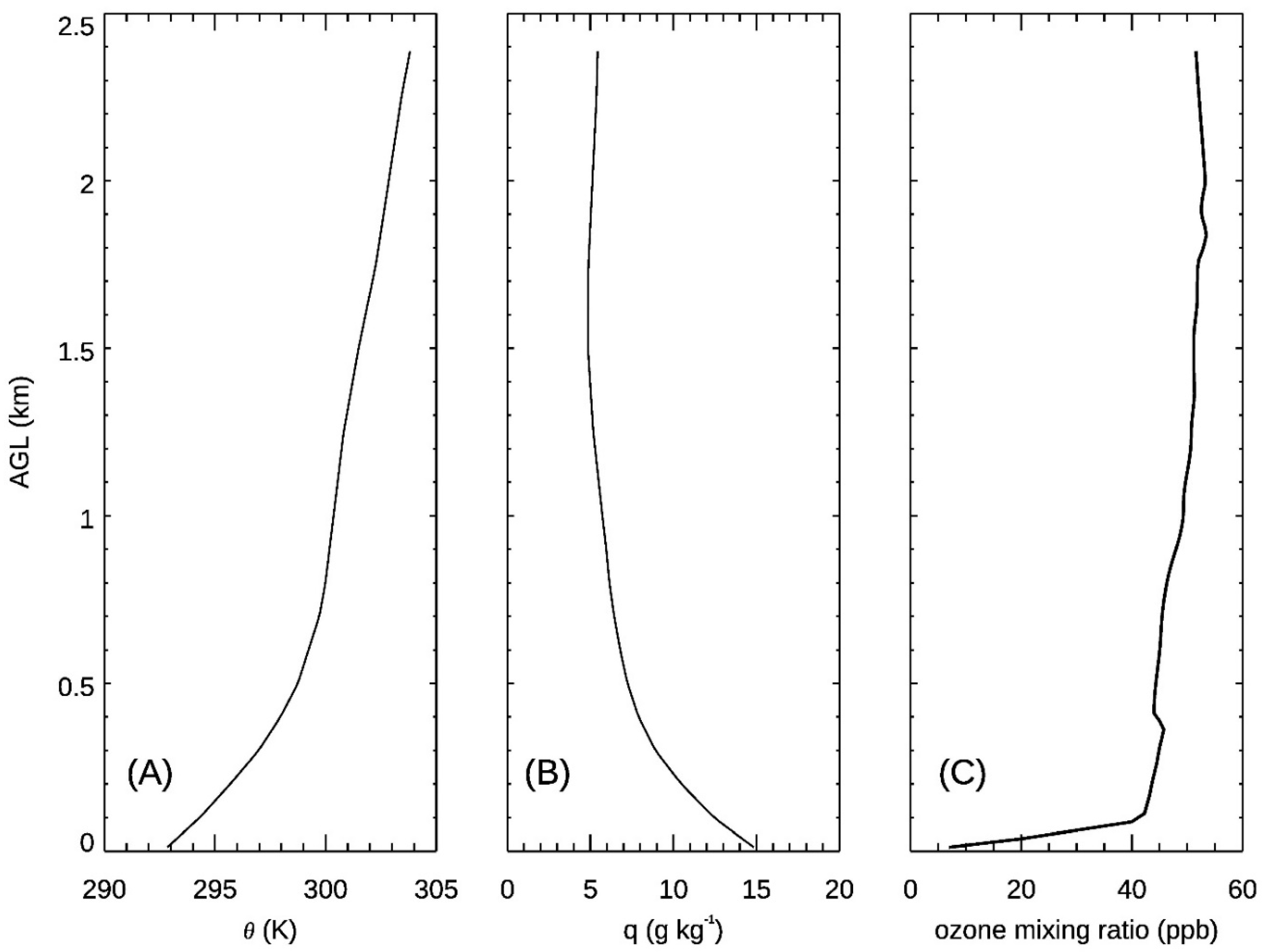
2.3.1. Physics Settings

The spatial resolution of the domain was set to 50 m × 50 m × 25 m in x, y, and z directions, respectively, with 100 × 100 × 96 grid cells in each dimension; consequently, the simulation domain was 5 km × 5 km × 2.4 km. The surface was assumed to be flat and homogenous. The total simulation time was set to 10 h with an adaptive time step of a maximum of 10 s for both chemistry and dynamics, which reduced the possibility of instabilities in the chemical solver and expensive computational costs. The fine temporal and spatial resolution resolved both atmospheric dynamical and chemical scales in the CBL. We used the parameterized radiation scheme of DALES that calculates radiative transfer at every single column of LES and neglects horizontal radiative transfer, which reduced our computational cost because our case was cloudless [37]. More details on the radiative transfer calculation can be found in [37]. We set the output intervals to 30 s.

To simulate the diurnal variation surface sensible and latent heat flux, both surface sensible and latent heat flux were set to 0.12 × SIN (SIN = sin(π × (time − 1380)/45,803)), where 1380 and 45,803 represented the sunset time at 1023 UTC and daytime length in seconds, respectively, and K∙ms⁻¹ and 0.0001 × SIN kg∙k⁻¹∙ms⁻¹, respectively. With no measurements of surface heat fluxes, these fluxes were based on climatology. Our simulation started at 10 UTC and warmed up our simulations during the first simulation hour. The geostrophic winds were set to zero and the initial profiles of potential temperature and water vapor were obtained from the collocated MIPS measurements, as shown in Figure 1 at 10 UTC. The first level meteorological data were obtained from surface measurements of MIPS. The initial ozone profiles were obtained from the RO₃QET DIAL, and the first level ozone input was obtained from the one hour ozone mixing ratio at 10 UTC, measured at the EPA air quality station located 6 km south of the ozone DIAL.

Because it plays an important role in the evolution of CBL in this case, it was also necessary to consider including large-scale subsidence in our simulations. We obtained the value of subsidence by analyzing the decrease of the residual layer (RL) between 11 and 17 UT, as shown in Figure 2 [44,58]. We assumed that the large-scale subsidence was approximately 0.009 m/s in all simulations because the RL decreased approximately 200 m over 6 h. It was noted that the constant large-scale subsidence in this study may have caused errors in our stimulation because the large-scale subsidence may vary during the day.

2.3.2. Chemistry Settings

The ozone chemistry that is typical for the Southeastern United States consists of very high VOC emissions, due to the dense forest coverage. Therefore, ozone production is controlled by the NOx concentration. The emission rate of isoprene and NO was set to 0.65 × SIN and 0.08 × COS (COS = (1 − cos(π × (time − 1380)/45,803))) ppb/s, respectively, based on the climatology of isoprene and NO emissions adjusted by previous studies [59,60,61].

Table 3. Initial inputs of reactive chemicals for all four cases. The rest of the chemical species are set to zero.

	Mixing Ratio (ppb, z < 200 m)	Mixing Ratio (ppb, z > 200 m)
Ozone	as Figure 1	as Figure 1
NO	0	0
NO2	1	0
ISO	2	0
HO2	0	0
OH	0	0
MVK	1.3	1.3
CH4	1724	1724
CO	124	124

shows the initial profiles of the chemical species. For comparison and understanding of the photochemical and entrainment contribution to CBL ozone enhancement, and in addition to the NO emission case just described, we also computed two numerical experiments with 50% and 100% more NO emission, respectively. We performed an additional numerical experiment turning off both chemistry and dry deposition results in four numerical experiments with the different NO emission rates of 0.08 × COS ppb/s, 0.12 × ppb/s NO, and 0.16 × COS ppb/s, and a control run with chemistry and dry deposition off, respectively, as shown in

Table 4. Overview experiments.

Name	Dynamics	Chemistry	Dry Depo.
Control	on	off	off
Std. NO emis.	on	on	on
150% NO emis.	on	on	on
200% NO emis.	on	on	on

.

3. Results and Discussions

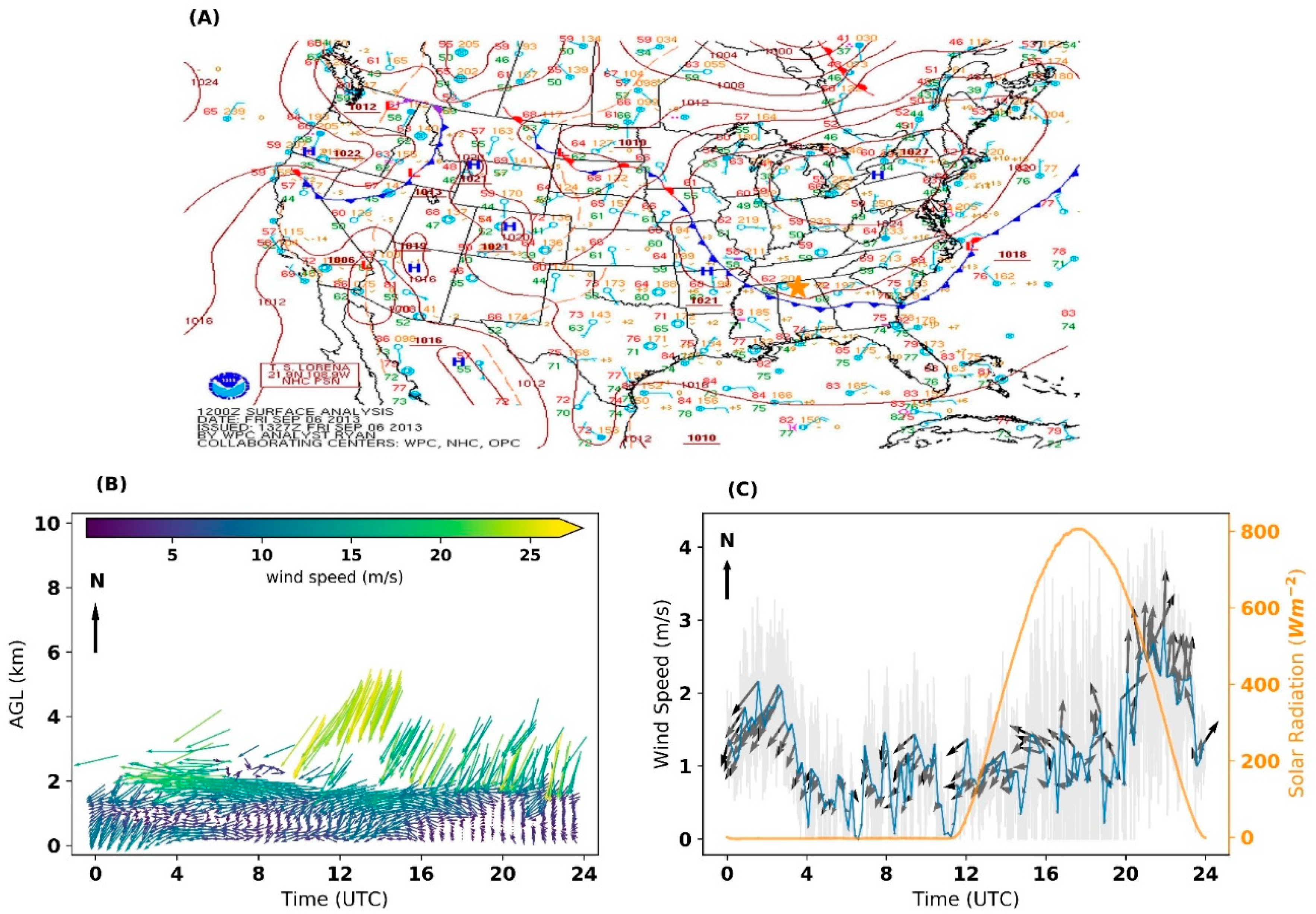
3.1. Meteorological Analysis

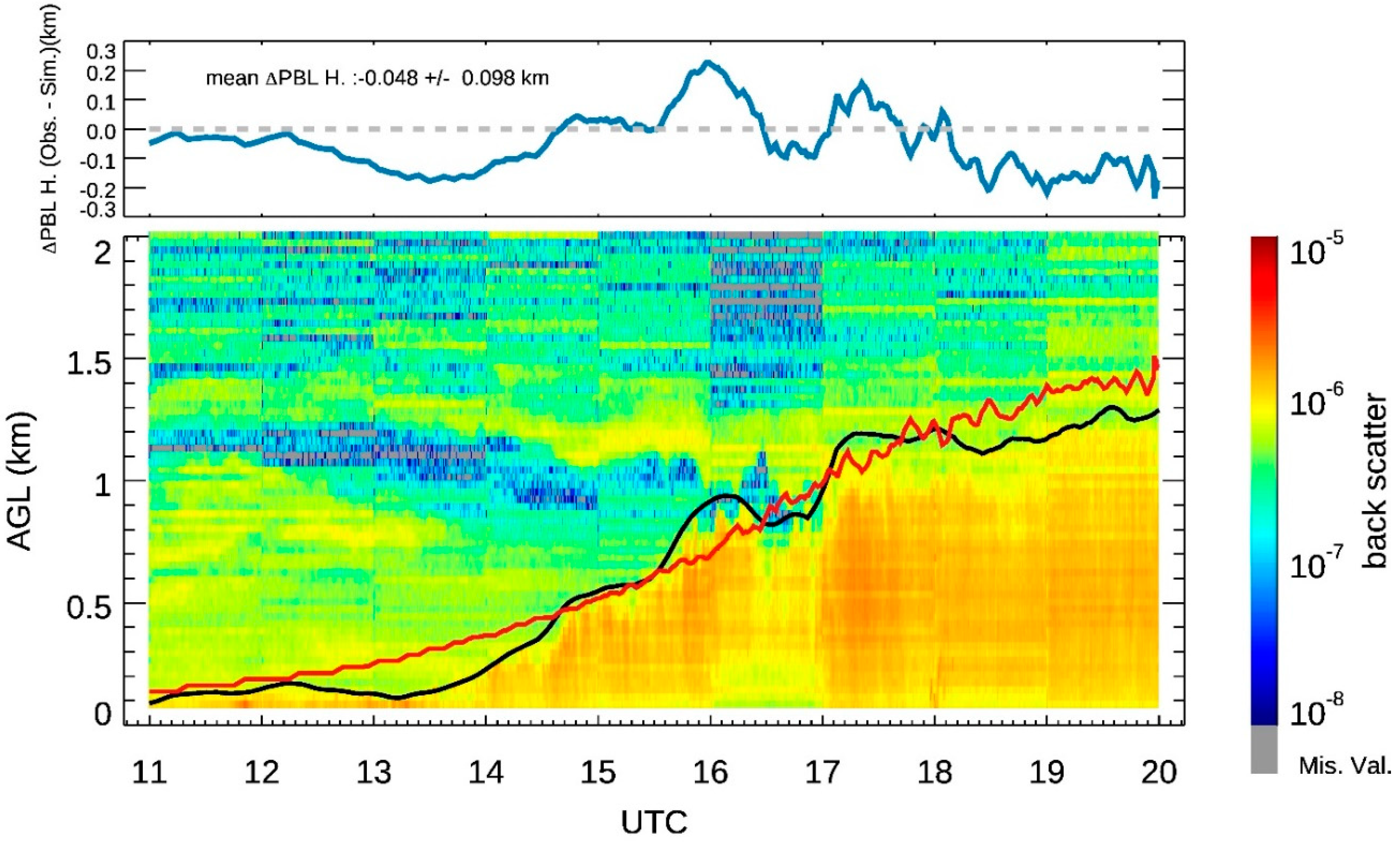
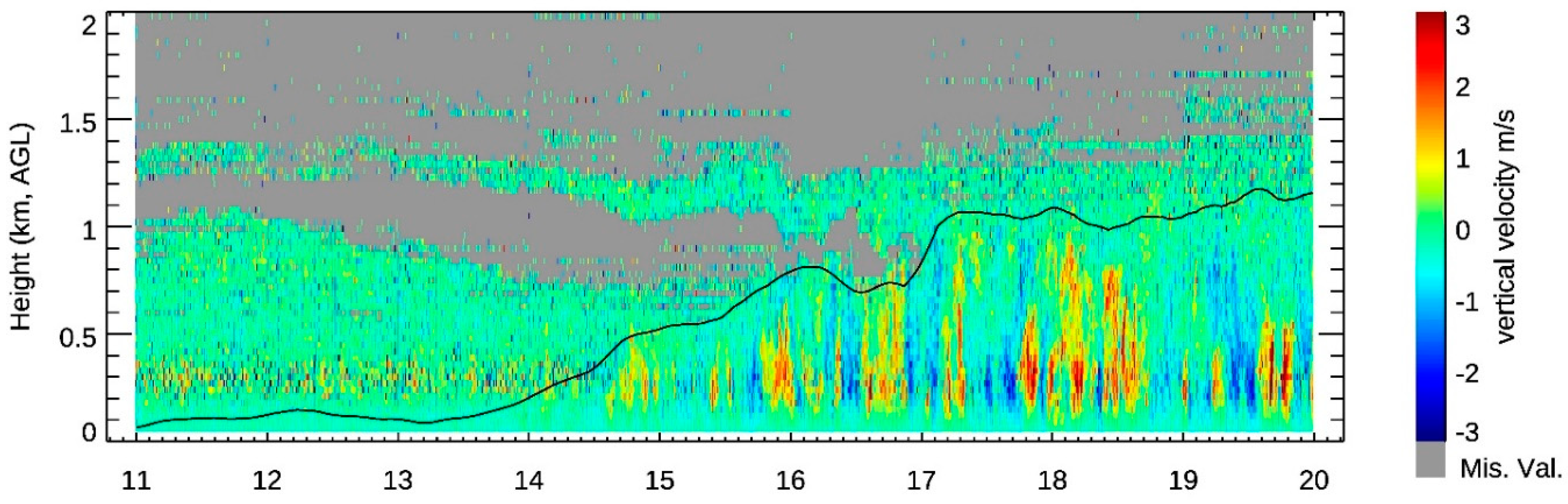
It is well known that meteorological fields play a critical role in the formation, transport, and deposition of air pollutants [62]. The surface analysis of the weather chart at UTC 1200 on 6 September 2013 clearly indicated that weather conditions in Huntsville, AL were controlled by an anticyclonic system, as shown in Panel (A) of Figure 3. The weather conditions in Huntsville were slightly windy with clear skies. The 10 m surface wind speed was low with less than 2 ms⁻¹ measured by surface instruments as shown in the bottom of Panel (C). Wind profiles observed by 915 MHz indicated the low wind speed in the CBL and the slightly increased wind speed above the CBL top, shown in Panel (B) of Figure 3. The solar radiation measured by the surface instruments in Panel (C) of Figure 3 show the diurnal curve of solar radiation without any interference from clouds. These weather conditions indicated that the horizontal ozone advection was too weak to transport the observed ozone amount to our study area, and the clear sky provided a large amount of solar radiation for photochemical production. Consequently, the ozone enhancement in the CBL on 6 September 2013 was mainly caused by local emissions and chemistry.

3.2. The CBL Height

The CBL height plays an important role in the ozone variation by diluting ozone concentrations and mixing air from the FT into the CBL through the entrainment processes. We applied the continuous wavelet transform (CWT) algorithm to determine the CBL heights based on the backscatter profile observed by CWAL with smoothing processes, as plotted by the solid black line in Figure 2 [4,63]. In addition, the simulated CBL heights from DALES, defined by the minimum local gradient of potential temperature profiles, are plotted by the solid red line in Figure 2. Generally, simulated CBL heights show acceptable agreement with the observed CBL heights, with slight underestimates. The mean differences between the observed and simulated CLB heights were 0.048 km with 0.098 km standard deviation. The DALES model successfully reproduced the evolution of CBL heights in the early morning. However, the model underestimated the CBL height between 1600 and 1700 UTC when an RL storing high aerosol concentrations at a 1.2–1.4 km height was incorporated into the growing CBL. The RL usually involved mean characteristics of the previous CBL including air pollutants, potential temperature, and relative humidity. When the potential temperature in the CBL reached the potential temperature in the RL, the CBL grew extremely fast by engulfing the RL. No (significant) inversion was present anymore between the growing CBL and the RL [27]. Consequently, the CBL height jump between 1600 and 1700 UTC was not captured by the DALES model. In addition, our simulation overestimated the CBL heights between 18 and 20 UTC because our constant large-scale subsidence assumption may have missed the variation of subsidence during our study period [11].

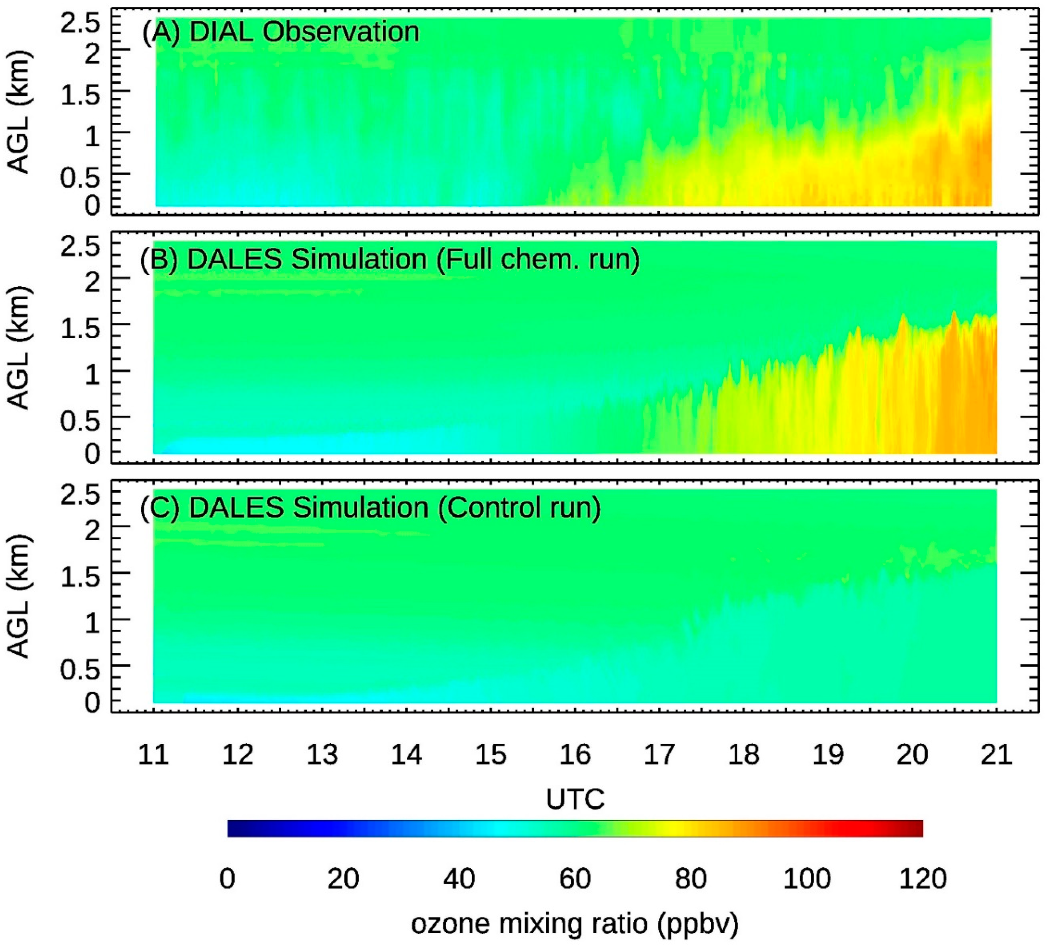
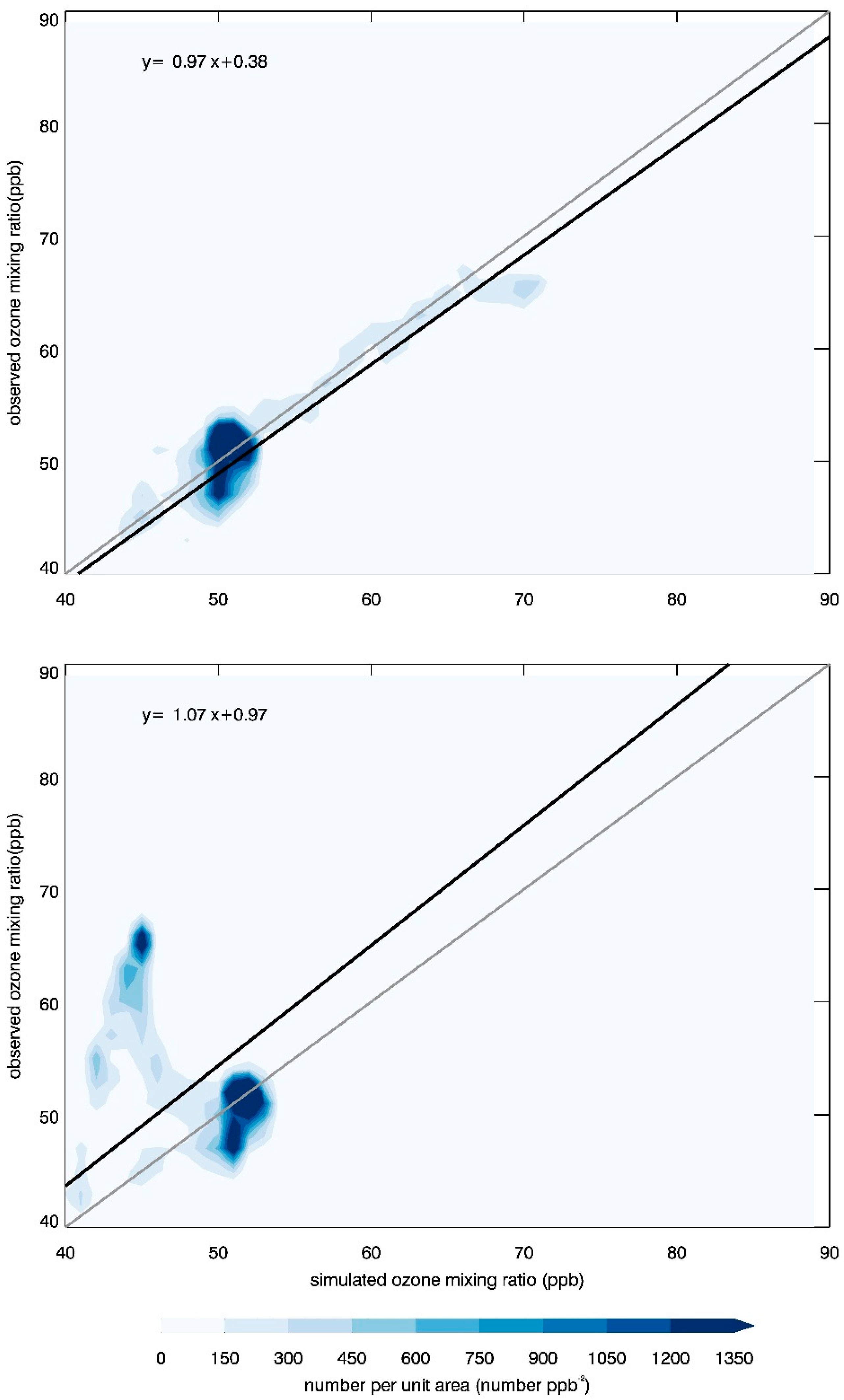
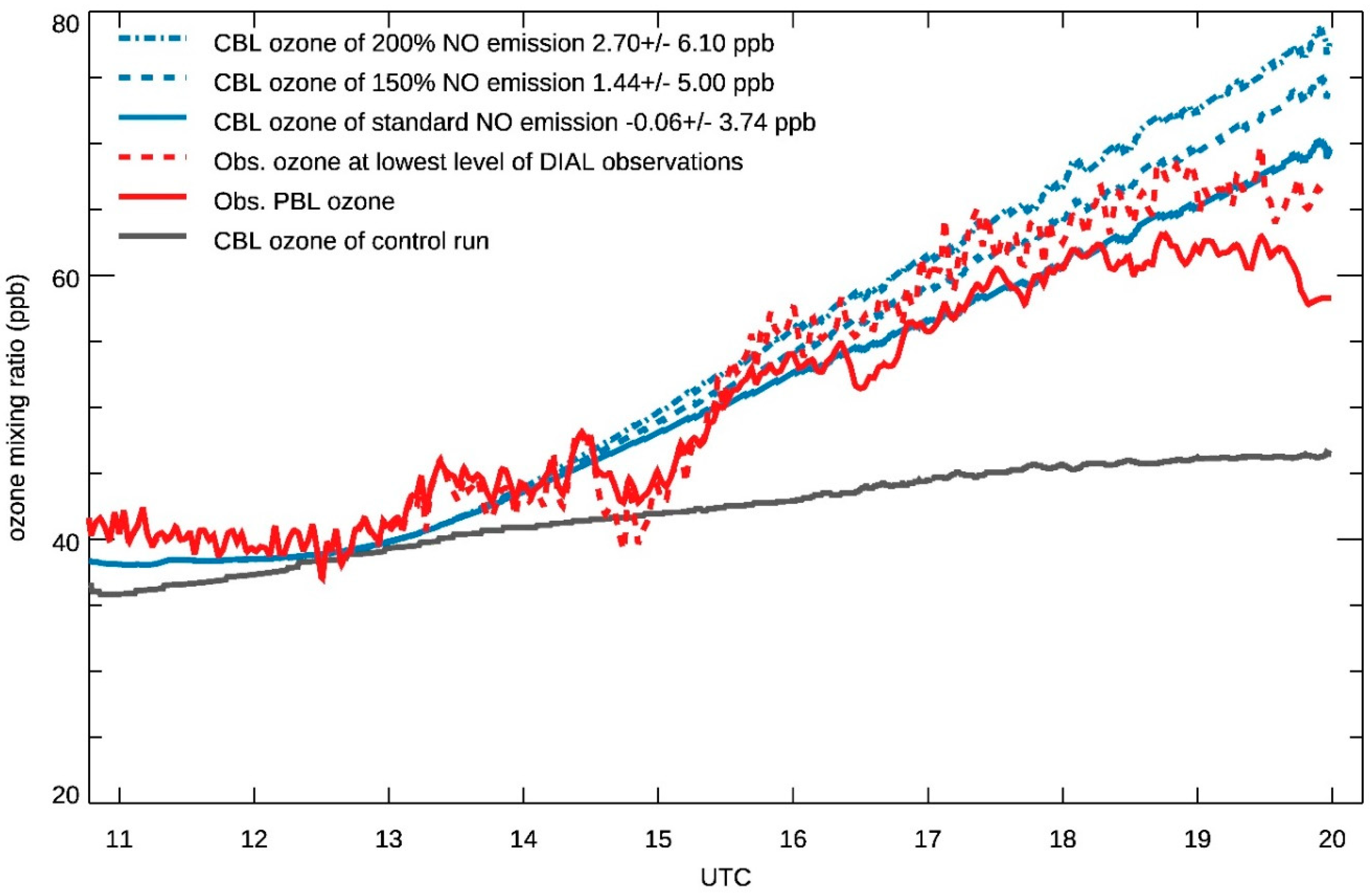
3.3. Ozone Variation in the CBL

In order to study ozone redistribution by eddy transport in the CBL without smoothing out the turbulence information, we investigated the ozone profiles at the center grid point of our domain with a 50 m horizontal and 25 m vertical resolution. The ozone observations from the ozone DIAL, simulation by DALES with standard NO emissions and a control run are plotted in Figure 4, from the top to the bottom panels, respectively. DALES reproduces the ozone temporal variation and the ozone structure caused by eddies in the CBL as shown in the top and middle panels in Figure 4. The DALES successfully reproduced the ozone variation and ozone morphology caused by eddies in the CBL, as shown in the middle panel of Figure 4. The ozone simulation of the control run in the bottom panel of Figure 4 implies that the ozone temporal variation on 6 September 2013 was caused mainly by local emissions and chemical production.

To quantify the comparisons between the ozone simulations and observations, we compared the model simulations with the observations between 0.1 and 2.375 km AGL in Figure 5. The top panel indicates the scatter plots of ozone DIAL observations and the standard NO emission simulation, while the bottom panel shows the comparisons between ozone DIAL observations and the DALES control run simulations. The DIAL observations had acceptable agreement with the DALES simulation, as shown in the top panel, with a slope of 0.97. In the bottom panel, the DALES control run reproduces the ozone mixing ratio in the FT as the hotspot pattern at ~50 ppb of simulated ozone and ~50 ppb of observed ozone, but underestimates the ozone in the CBL as the hotspot pattern at ~45 ppb of simulated ozone and ~68 ppb of observed ozone mixing ratio.

The comparisons between simulated and observed CBL ozone values are shown in Figure 6. The simulated and observed CBL ozone values were calculated by integrating the bottom to the corresponding CBL top. We noted that all simulated CBL ozone mixing ratios averaged over the whole domain to avoid the high frequency noise. The CBL ozone simulation with standard NO emission indicated acceptable agreement with our DIAL observations with a −0.06 ppb mean bias and a 3.74 ppb standard deviation during our study period. Large CBL ozone biases between the simulation and the observation occurred at 15, 16.5–17 and ~18–20 UTC, when the DALES missed the CBL heights. We also did a sensitivity test on ozone production rates with different NO emissions. The average ozone production rates in the CBL were 3.8, 4.2 and 4.5 ppb/hour for the standard, 150%, and 200% NO emissions, respectively.

The total ozone enhancement, defined by the difference between mean CBL ozone at 11–12 UTC and 19–20 UTC was ~18 ppb, observed by our DIAL and ~27 ppb by our simulation with standard NO emissions. Our control run showed a ~5 ppb increase in CBL ozone values caused by the mixing of low ozone air in the FT through entrainment processes and other physical processes. Consequently, about two thirds of the CBL ozone enhancement based on our DIAL observations was caused by photochemical reactions from local emissions and pollutions and the remaining one third was caused by dynamical transport in this study.

This agreement between ozone DIAL observations and DALES simulations indicated that the dry deposition module helped improve our simulations, but it is challenging to quantify how much of the improvement can be attributed to the dry deposition module due to the fact that: (1) ozone flux at heights below 500 m contains high uncertainties (discussed in Section 3.4); (2) ozone measurements at ground level collocated with the DIAL were insufficient; and (3) land surface in our domain is heterogenous while our simulations use a homogeneous surface. Our future studies will investigate the dry deposition and its impact on the CBL ozone variation.

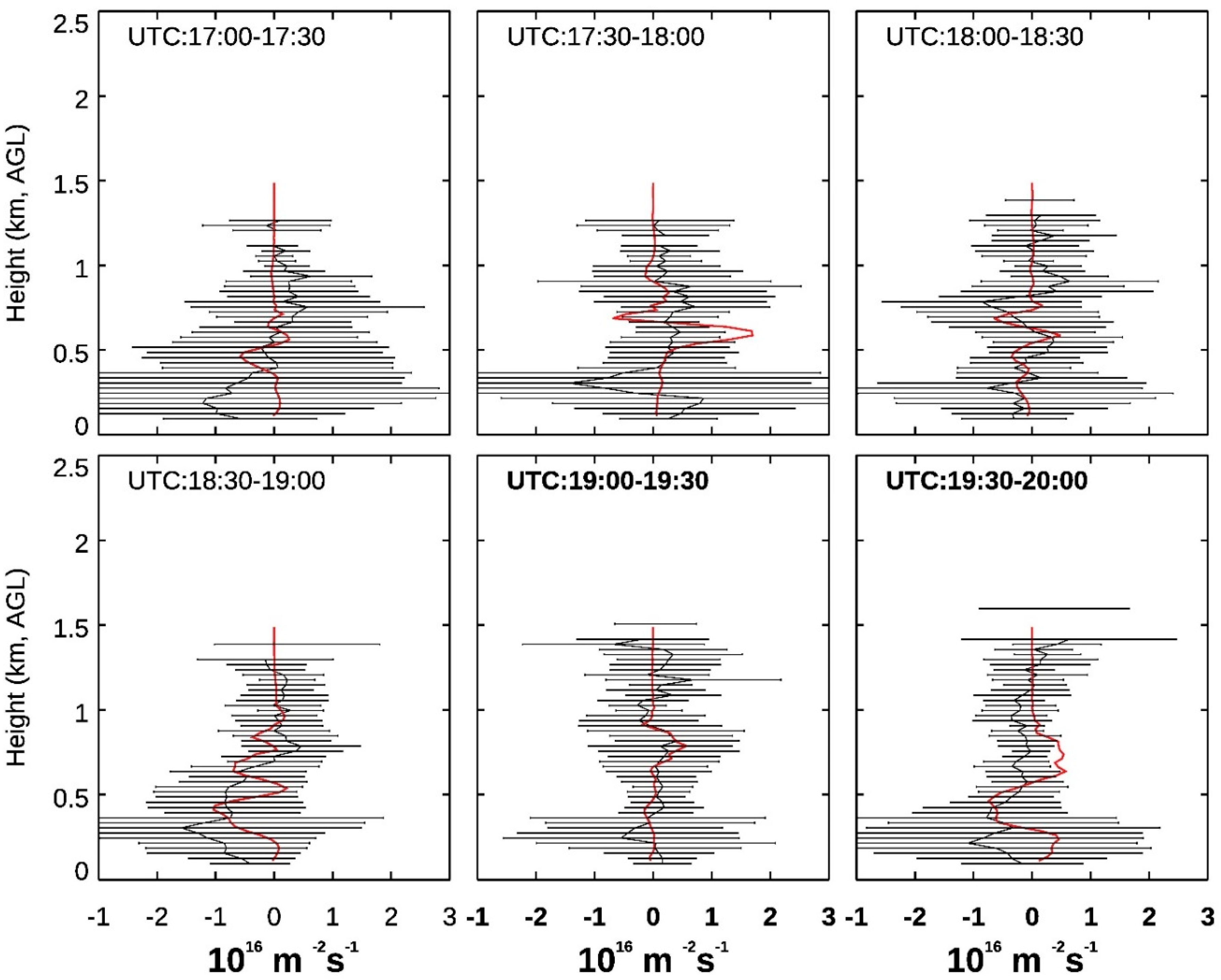
3.4. Ozone Transport within the CBL

Ozone transport within the CBL is a significant process for both ground ozone concentrations and the CBL budget. The land surface can provide either strong ozone sinks by deposition processes or strong ozone production sources through high emissions. The redistribution of ozone in the CBL occurs through convective mixing; the interaction between the CBL and the ground ozone concentration occurs through turbulent flux. For the calculation of the turbulence’s impacts on ozone, we need to investigate the highly resolved time series of vertical wind velocity and ozone mixing ratio data at specific height levels. We applied Taylor’s frozen turbulence hypothesis: the temporally-averaged observations can represent the corresponding spatial average observations [50]. Then, the turbulent ozone flux was defined as $\overline{w^{\prime }{O}_3{}^{\prime }}$, where the prime represents deviations from the mean value, and the overbar represents the temporal average.

The vertical wind profiles observed by CWAL are plotted in Figure 7. After the sunrise, eddies started to grow vertically due to the increased surface heat flux, as shown in Figure 7. The persistent layer of noise at approximately 300 m AGL throughout our observations was associated with a possible remnant warm plume atop the relatively warmer building and a more urbanized area around the campus [34].

The statistical errors of the ozone flux, due to noise, were taken into account. The measured ozone flux is written as [64]:

$${\overline{{\mathrm{w}{}^{\prime }\mathrm{O}}_3{}^{\prime }}}_{\mathrm{m}}=\overline{{\mathrm{w}{}^{\prime }\mathrm{O}}_3{}^{\prime }}+\overline{{\mathsf{\delta }\mathrm{w}{}^{\prime }\mathrm{O}}_3{}^{\prime }}+\overline{{\mathrm{w}{}^{\prime }\mathsf{\delta }\mathrm{O}}_3{}^{\prime }}+\overline{{\mathsf{\delta }\mathrm{w}{}^{\prime }\mathsf{\delta }\mathrm{O}}_3{}^{\prime }},$$

(5)

where δw′ and δO₃′ are fluctuations of the vertical wind and ozone mixing ratio, respectively. The variance of the measured ozone flux caused by system noise can be expressed as [64]:

$${\mathsf{\sigma }}^2\left({\overline{{\mathrm{w}{}^{\prime }\mathrm{O}}_3{}^{\prime }}}_{\mathrm{m}}\right)={\mathsf{\sigma }}^2\left(\overline{{\mathsf{\delta }\mathrm{w}{}^{\prime }\mathrm{O}}_3{}^{\prime }}+\overline{{\mathrm{w}{}^{\prime }\mathsf{\delta }\mathrm{O}}_3{}^{\prime }}+\overline{{\mathsf{\delta }\mathrm{w}{}^{\prime }\mathsf{\delta }\mathrm{O}}_3{}^{\prime }}\right)=\frac{1}{N}\left({\overline{O_{3 }^{{}^{\prime }2}}}_m \overline{{\delta }^{2}w{}^{\prime }}+ \overline{{\delta }^2{O}_3^{{}^{\prime }}} {\overline{w^{{}^{\prime }2}}}_m+\overline{{\delta }^2{O}_3^{{}^{\prime }}} \overline{{\delta }^{2}w{}^{\prime }}\right).$$

(6)

We calculated the observed ozone turbulent flux (solid black line) with statistical errors at each level (horizontal black line) every 30 min from 1700–200 UTC (shown in Figure 8), as well as the simulated ozone turbulent flux (solid red line). It is evident that the spatial and temporal resolutions of ozone DIAL and CWAL are not fine enough to capture the ozone flux caused by small eddies (with lengths less than the measurement resolution). Consequently, ozone flux may be underestimated. However, the ignored portion of the ozone flux should be negligible in the CBL. The unresolved part of the ozone flux cannot be quantified since there is no high resolution in situ measurement on both ozone and wind with for comparison with the measurements by ground-based remote-sensing techniques [65].

The statistical errors were significantly larger at approximately 200–500 m AGL for each panel in Figure 8, possibly because of a remnant warm plume from the relatively warmer building and a more urbanized area around the campus [34]. The majority of the simulated ozone fluxes above 500 m AGL were within the range of observed ozone fluxes plus or minus statistical errors. This indicated that the DALES reproduced the typical ozone behavior for a clear late summer day—the CBL ozone mixing ratio increases during the daytime due to local production with sunlight presence. The knowledge of the vertical distribution of the ozone mixing ratio in the CBL and RL allowed some basic predictions about the turbulent fluxes associated with this ozone vertical distribution. The ground is known to be an ozone sink due to the dry deposition, while the photochemical production of ozone in the CBL under clear summer conditions acted as a source of ozone. This caused a slightly higher ozone mixing ratio in the CBL than at the ground surface. Therefore, the observed ozone fluxes indicated downward motion at each time interval.

4. Conclusions

We investigated the diurnal ozone evolution on 6 September 2013 in Huntsville, Alabama, using multiple measurements and the DALES model coupled with a chemical module. In addition, a dry deposition scheme was also added in this study. The DALES successfully reproduced the CBL ozone enhancement from the local emissions and chemical productions. The experiments between the chemical and control run (with chemistry off) suggested that the ozone production was controlled mainly by local emissions on this particular day with low horizontal winds and strong solar insolation, in this case. This study indicated that the LES model and lidar observations, in high temporal and spatial resolution, are powerful tools to help us understand ozone and other air pollutant variations in the CBL.

The CBL height was determined by finding the highest gradients in the CWAL backscatter profiles using the continuous wavelet transform technique. Generally, the DALES-simulated CBL heights have acceptable agreement with the observed CBL heights. The two reasons that the model missed the CBL heights are: the intrusion of the RL and the variation of large-scale subsidence. The CBL height grows fast when an RL storing low ozone concentration is incorporated into the growing CBL through the entrainment. In addition, our constant large-scale settings may have missed the evolution of the large-scale on that day, resulting in the underestimate of CBL height in the late afternoon.

References

1. Jenkin, M.E.; Clemitshaw, K.C. Ozone and other secondary photochemical pollutants: chemical processes governing their formation in the planetary boundary layer. Atmos. Environ. 2000, 34, 2499–2527. [Google Scholar] [CrossRef]
2. EPA (Ed.) EPA’s Reports on the Environment; United States Environmental Protection Agency: Washington, DC, USA, 2008; p. 366.
3. Kuang, S.; Newchurch, M.J.; Burris, J.; Wang, L.; Buckley, P.I.; Johnson, S.; Knupp, K.; Huang, G.; Phillips, D.; Cantrell, W. Nocturnal ozone enhancement in the lower troposphere observed by lidar. Atmos. Environ. 2011, 45, 6078–6084. [Google Scholar] [CrossRef]
4. Huang, G.; Newchurch, M.J.; Kuang, S.; Buckley, P.I.; Cantrell, W.; Wang, L. Definition and determination of ozone laminae using Continuous Wavelet Transform (CWT) analysis. Atmos. Environ. 2015, 104, 125–131. [Google Scholar] [CrossRef]
5. Kuang, S.; Newchurch, M.J.; Burris, J.; Wang, L.; Knupp, K.; Huang, G. Stratosphere-to-troposphere transport revealed by ground-based lidar and ozonesonde at a midlatitude site. J. Geophys. Res.-Atmos. 2012, 117. [Google Scholar] [CrossRef] [Green Version]
6. Tong, N.O.; Leung, D.C.; Liu, C.-H. A Review on Ozone Evolution and Its Relationship with Boundary Layer Characteristics in Urban Environments. Water Air Soil Pollut. 2011, 214, 13–36. [Google Scholar] [CrossRef]
7. Jaffe, D.A.; Wigder, N.L. Ozone production from wildfires: A critical review. Atmos. Environ. 2012, 51, 1–10. [Google Scholar] [CrossRef]
8. Langford, A.O.; Brioude, J.; Cooper, O.R.; Senff, C.J.; Alvarez, R.J., II; Hardesty, R.M.; Johnson, B.J.; Oltmans, S.J. Stratospheric influence on surface ozone in the Los Angeles area during late spring and early summer of 2010. J. Geophys. Res. 2012, 117, D00V06. [Google Scholar] [CrossRef]
9. Duncan, B.N.; Yoshida, Y.; Olson, J.R.; Sillman, S.; Martin, R.V.; Lamsal, L.; Hu, Y.; Pickering, K.E.; Retscher, C.; Allen, D.J.; et al. Application of OMI observations to a space-based indicator of NOx and VOC controls on surface ozone formation. Atmos. Environ. 2010, 44, 2213–2223. [Google Scholar] [CrossRef] [Green Version]
10. Sillman, S.; Al-Wali, K.I.; Marsik, F.J.; Nowacki, P.; Samson, P.J.; Rodgers, M.O.; Garland, L.J.; Martinez, J.E.; Stoneking, C.; Imhoff, R.; et al. Photochemistry of ozone formation in Atlanta, GA-Models and measurements. Atmos. Environ. 1995, 29, 3055–3066. [Google Scholar] [CrossRef]
11. Blanchard, C.L.; Hidy, G.M.; Tanenbaum, S. Ozone in the southeastern United States: An observation-based model using measurements from the SEARCH network. Atmos. Environ. 2014, 88, 192–200. [Google Scholar] [CrossRef]
12. Hidy, G.M. Ozone process insights from field experiments—Part I: overview. Atmos. Environ. 2000, 34, 2001–2022. [Google Scholar] [CrossRef]
13. Zhang, Y.; Bocquet, M.; Mallet, V.; Seigneur, C.; Baklanov, A. Real-time air quality forecasting, part II: State of the science, current research needs, and future prospects. Atmos. Environ. 2012, 60, 656–676. [Google Scholar] [CrossRef]
14. Yegorova, E.A.; Allen, D.J.; Loughner, C.P.; Pickering, K.E.; Dickerson, R.R. Characterization of an eastern U.S. severe air pollution episode using WRF/Chem. J. Geophys. Res.-Atmos. 2011, 116, D17306. [Google Scholar] [CrossRef]
15. Castellanos, P.; Marufu, L.T.; Doddridge, B.G.; Taubman, B.F.; Schwab, J.J.; Hains, J.C.; Ehrman, S.H.; Dickerson, R.R. Ozone, oxides of nitrogen, and carbon monoxide during pollution events over the eastern United States: An evaluation of emissions and vertical mixing. J. Geophys. Res.-Atmos. 2011, 116, D16307. [Google Scholar] [CrossRef]
16. So, K.L.; Wang, T. On the local and regional influence on ground-level ozone concentrations in Hong Kong. Environ. Pollut. 2003, 123, 307–317. [Google Scholar] [CrossRef] [Green Version]
17. Shao, M.; Zhang, Y.; Zeng, L.; Tang, X.; Zhang, J.; Zhong, L.; Wang, B. Ground-level ozone in the Pearl River Delta and the roles of VOC and NOx in its production. J. Environ. Manag. 2009, 90, 512–518. [Google Scholar] [CrossRef]
18. Chance, K.; Liu, X.; Suleiman, R.M.; Flittner, D.E.; Al-Saadi, J.; Janz, S.J. Tropospheric Emissions: Monitoring of Pollution (TEMPO); SPIE: Bellingham, WA, USA, 2013; Volume 8866. [Google Scholar]
19. Zoogman, P.; Liu, X.; Suleiman, R.M.; Pennington, W.F.; Flittner, D.E.; Al-Saadi, J.A.; Hilton, B.B.; Nicks, D.K.; Newchurch, M.J.; Carr, J.L.; et al. Tropospheric emissions: Monitoring of pollution (TEMPO). J. Quant. Spectrosc. Radiat. Transf. 2017, 186, 17–39. [Google Scholar] [CrossRef] [Green Version]
20. Martins, D.K.; Stauffer, R.M.; Thompson, A.M.; Halliday, H.S.; Kollonige, D.; Joseph, E.; Weinheimer, A.J. Ozone correlations between mid-tropospheric partial columns and the near-surface at two mid-atlantic sites during the DISCOVER-AQ campaign in July 2011. J. Atmos. Chem. 2013, 1–19. [Google Scholar] [CrossRef]
21. Goldberg, D.L.; Loughner, C.P.; Tzortziou, M.; Stehr, J.W.; Pickering, K.E.; Marufu, L.T.; Dickerson, R.R. Higher surface ozone concentrations over the Chesapeake Bay than over the adjacent land: Observations and models from the DISCOVER-AQ and CBODAQ campaigns. Atmos. Environ. 2014, 84, 9–19. [Google Scholar] [CrossRef]
22. Peterson, D.A.; Hyer, E.J.; Campbell, J.R.; Fromm, M.D.; Hair, J.W.; Butler, C.F.; Fenn, M.A. The 2013 Rim Fire: Implications for Predicting Extreme Fire Spread, Pyroconvection, and Smoke Emissions. Bull. Am. Meteorol. Soc. 2014. [Google Scholar] [CrossRef]
23. Duncan, B.N.; Prados, A.I.; Lamsal, L.N.; Liu, Y.; Streets, D.G.; Gupta, P.; Hilsenrath, E.; Kahn, R.A.; Nielsen, J.E.; Beyersdorf, A.J.; et al. Satellite data of atmospheric pollution for U.S. air quality applications: Examples of applications, summary of data end-user resources, answers to FAQs, and common mistakes to avoid. Atmos. Environ. 2014, 94, 647–662. [Google Scholar] [CrossRef] [Green Version]
24. Fishman, J.; Iraci, L.T.; Al-Saadi, J.; Chance, K.; Chavez, F.; Chin, M.; Coble, P.; Davis, C.; DiGiacomo, P.M.; Edwards, D.; et al. The United States’ Next Generation of Atmospheric Composition and Coastal Ecosystem Measurements: NASA’s Geostationary Coastal and Air Pollution Events (GEO-CAPE) Mission. Bull. Am. Meteorol. Soc. 2012, 93, 1547–1566. [Google Scholar] [CrossRef]
25. van Stratum, B.J.H.; Vilà-Guerau de Arellano, J.; Ouwersloot, H.G.; van den Dries, K.; van Laar, T.W.; Martinez, M.; Lelieveld, J.; Diesch, J.M.; Drewnick, F.; Fischer, H.; et al. Case study of the diurnal variability of chemically active species with respect to boundary layer dynamics during DOMINO. Atmos. Chem. Phys. 2012, 12, 5329–5341. [Google Scholar] [CrossRef] [Green Version]
26. Chamecki, M.; Meneveau, C.; Parlange, M.B. Large eddy simulation of pollen transport in the atmospheric boundary layer. J. Aerosol Sci. 2009, 40, 241–255. [Google Scholar] [CrossRef] [Green Version]
27. Ouwersloot, H.G.; Vilà-Guerau de Arellano, J.; Nölscher, A.C.; Krol, M.C.; Ganzeveld, L.N.; Breitenberger, C.; Mammarella, I.; Williams, J.; Lelieveld, J. Characterization of a boreal convective boundary layer and its impact on atmospheric chemistry during HUMPPA-COPEC-2010. Atmos. Chem. Phys. 2012, 12, 9335–9353. [Google Scholar] [CrossRef] [Green Version]
28. Langford, A.O.; Tucker, S.C.; Senff, C.J.; Banta, R.M.; Brewer, W.A.; Alvarez, R.J., II; Hardesty, R.M.; Lerner, B.M.; Williams, E.J. Convective venting and surface ozone in Houston during TexAQS 2006. J. Geophys. Res. 2010, 115, D16305. [Google Scholar] [CrossRef]
29. Senff, C.J.; Alvarez, R.J., II; Hardesty, R.M.; Banta, R.M.; Langford, A.O. Airborne lidar measurements of ozone flux downwind of Houston and Dallas. J. Geophys. Res. 2010, 115, D20307. [Google Scholar] [CrossRef]
30. Kuang, S.; Newchurch, M.J.; Johnson, M.S.; Wang, L.; Burris, J.; Pierce, R.B.; Eloranta, E.W.; Pollack, I.B.; Graus, M.; de Gouw, J.; et al. Summertime tropospheric ozone enhancement associated with a cold front passage due to stratosphere-to-troposphere transport and biomass burning: simultaneous ground-based lidar and airborne measurements. J. Geophys. Res.-Atmos. 2017. [Google Scholar] [CrossRef]
31. Kuang, S.; Newchurch, M.J.; Burris, J.; Liu, X. Ground-based lidar for atmospheric boundary layer ozone measurements. Appl. Opt. 2013, 52, 3557–3566. [Google Scholar] [CrossRef]
32. Kuang, S.; Burris, J.F.; Newchurch, M.J.; Johnson, S.; Long, S. Differential Absorption Lidar to Measure Subhourly Variation of Tropospheric Ozone Profiles. IEEE Trans. Geosci. Remote Sens. 2011, 49, 557–571. [Google Scholar] [CrossRef] [Green Version]
33. Karan, H.; Knupp, K. Mobile Integrated Profiler System (MIPS) Observations of Low-Level Convergent Boundaries during IHOP. Mon. Weather Rev. 2006, 134, 92–112. [Google Scholar] [CrossRef]
34. Wingo, S.M.; Knupp, K.R. Multi-platform Observations Characterizing the Afternoon-to-Evening Transition of the Planetary Boundary Layer in Northern Alabama, USA. Bound. -Layer Meteorol. 2014, 155, 29–53. [Google Scholar] [CrossRef] [Green Version]
35. Busse, J.; Knupp, K. Observed Characteristics of the Afternoon–Evening Boundary Layer Transition Based on Sodar and Surface Data. J. Appl. Meteorol. Climatol. 2012, 51, 571–582. [Google Scholar] [CrossRef]
36. Knupp, K.R.; Coleman, T.; Phillips, D.; Ware, R.; Cimini, D.; Vandenberghe, F.; Vivekanandan, J.; Westwater, E. Ground-Based Passive Microwave Profiling during Dynamic Weather Conditions. J. Atmos. Ocean. Technol. 2009, 26, 1057–1073. [Google Scholar] [CrossRef]
37. Heus, T.; van Heerwaarden, C.C.; Jonker, H.J.J.; Pier Siebesma, A.; Axelsen, S.; van den Dries, K.; Geoffroy, O.; Moene, A.F.; Pino, D.; de Roode, S.R.; et al. Formulation of the Dutch Atmospheric Large-Eddy Simulation (DALES) and overview of its applications. Geosci. Model Dev. 2010, 3, 415–444. [Google Scholar] [CrossRef] [Green Version]
38. Böing, S.J.; Jonker, H.J.J.; Siebesma, A.P.; Grabowski, W.W. Influence of the Subcloud Layer on the Development of a Deep Convective Ensemble. J. Atmos. Sci. 2012, 69, 2682–2698. [Google Scholar] [CrossRef] [Green Version]
39. Vilà-Guerau de Arellano, J.; Kim, S.W.; Barth, M.C.; Patton, E.G. Transport and chemical transformations influenced by shallow cumulus over land. Atmos. Chem. Phys. 2005, 5, 3219–3231. [Google Scholar] [CrossRef] [Green Version]
40. Ouwersloot, H.G. The Impact of Dynamic Processes on Chemistry in Atmospheric Boundary Layers over Tropical and Boreal Forest; Wageningen University: Wageningen, The Netherlands, 2013. [Google Scholar]
41. Aan de Brugh, J.M.J.; Ouwersloot, H.G.; Vilà-Guerau de Arellano, J.; Krol, M.C. A large-eddy simulation of the phase transition of ammonium nitrate in a convective boundary layer. J. Geophys. Res.-Atmos. 2013, 118, 826–836. [Google Scholar] [CrossRef] [Green Version]
42. Ouwersloot, H.G.; Vilà-Guerau de Arellano, J.; van Heerwaarden, C.C.; Ganzeveld, L.N.; Krol, M.C.; Lelieveld, J. On the segregation of chemical species in a clear boundary layer over heterogeneous land surfaces. Atmos. Chem. Phys. 2011, 11, 10681–10704. [Google Scholar] [CrossRef] [Green Version]
43. Vilà-Guerau de Arellano, J.; van den Dries, K.; Pino, D. On inferring isoprene emission surface flux from atmospheric boundary layer concentration measurements. Atmos. Chem. Phys. 2009, 9, 3629–3640. [Google Scholar] [CrossRef] [Green Version]
44. Blay-Carreras, E.; Pino, D.; Vilà-Guerau de Arellano, J.; van de Boer, A.; De Coster, O.; Darbieu, C.; Hartogensis, O.; Lohou, F.; Lothon, M.; Pietersen, H. Role of the residual layer and large-scale subsidence on the development and evolution of the convective boundary layer. Atmos. Chem. Phys. 2014, 14, 4515–4530. [Google Scholar] [CrossRef] [Green Version]
45. Dlugi, R.; Berger, M.; Zelger, M.; Hofzumahaus, A.; Rohrer, F.; Holland, F.; Lu, K.; Kramm, G. The balances of mixing ratios and segregation intensity: A case study from the field (ECHO 2003). Atmos. Chem. Phys. 2014, 14, 10333–10362. [Google Scholar] [CrossRef]
46. Vilà-Guerau de Arellano, J.; Patton, E.G.; Karl, T.; van den Dries, K.; Barth, M.C.; Orlando, J.J. The role of boundary layer dynamics on the diurnal evolution of isoprene and the hydroxyl radical over tropical forests. J. Geophys. Res. 2011, 116, D07304. [Google Scholar] [CrossRef]
47. Wesely, M.L.; Hicks, B.B. A review of the current status of knowledge on dry deposition. Atmos. Environ. 2000, 34, 2261–2282. [Google Scholar] [CrossRef]
48. Seinfeld, J.H.; Pandis, S.N. Atmospheric Chemistry and Physics: From Air Pollution to Climate Change, 2nd ed.; John Wiley & Sons: Hoboken, NJ, USA, 2006. [Google Scholar]
49. Biazar, A.P. The Role of Natural Nitrogen Oxides in Ozone Production in the Southeastern Environment. Ph.D. Thesis, The University of Alabama in Huntsville, Ann Arbor, MI, USA, 1995. [Google Scholar]
50. Stull, R.B. An Introduction to Boundary Layer Meteorology; Springer: Berlin, Germany, 1988; Volume 13. [Google Scholar]
51. Dentener, F.; Vet, R.; Dennis, R.L.; Du, E.; Kulshrestha, U.C.; Galy-Lacaux, C. Progress in Monitoring and Modelling Estimates of Nitrogen Deposition at Local, Regional and Global Scales. In Nitrogen Deposition, Critical Loads and Biodiversity; Sutton, M.A., Mason, K.E., Sheppard, L.J., Sverdrup, H., Haeuber, R., Hicks, W.K., Eds.; Springer: Dordrecht, The Netherlands, 2014; pp. 7–22. [Google Scholar]
52. Erisman, J.W.; Van Pul, A.; Wyers, P. Parametrization of surface resistance for the quantification of atmospheric deposition of acidifying pollutants and ozone. Atmos. Environ. 1994, 28, 2595–2607. [Google Scholar] [CrossRef]
53. Ganzeveld, L.; Lelieveld, J. Dry deposition parameterization in a chemistry general circulation model and its influence on the distribution of reactive trace gases. J. Geophys. Res. 1995, 100, 20999. [Google Scholar] [CrossRef] [Green Version]
54. Pleim, J.E.; Xiu, A.; Finkelstein, P.L.; Otte, T.L. A Coupled Land-Surface and Dry Deposition Model and Comparison to Field Measurements of Surface Heat, Moisture, and Ozone Fluxes. Water Air Soil Pollut. Focus 2001, 1, 243–252. [Google Scholar] [CrossRef]
55. Zhang, L.; Moran, M.D.; Makar, P.A.; Brook, J.R.; Gong, S. Modelling gaseous dry deposition in AURAMS: A unified regional air-quality modelling system. Atmos. Environ. 2002, 36, 537–560. [Google Scholar] [CrossRef]
56. Zhang, L.; Brook, J.R.; Vet, R. A revised parameterization for gaseous dry deposition in air-quality models. Atmos. Chem. Phys. 2003, 3, 2067–2082. [Google Scholar] [CrossRef] [Green Version]
57. Sickles Ii, J.E.; Shadwick, D.S. Air quality and atmospheric deposition in the eastern US: 20 years of change. Atmos. Chem. Phys. 2015, 15, 173–197. [Google Scholar] [CrossRef] [Green Version]
58. Yi, C.; Davis, K.J.; Berger, B.W.; Bakwin, P.S. Long-Term Observations of the Dynamics of the Continental Planetary Boundary Layer. J. Atmos. Sci. 2001, 58, 1288–1299. [Google Scholar] [CrossRef]
59. Geron, C.D.; Nie, D.; Arnts, R.R.; Sharkey, T.D.; Singsaas, E.L.; Vanderveer, P.J.; Guenther, A.; Sickles, J.E.; Kleindienst, T.E. Biogenic isoprene emission: Model evaluation in a southeastern United States bottomland deciduous forest. J. Geophys. Res. 1997, 102, 18889. [Google Scholar] [CrossRef]
60. Kesselmeier, J.; Staudt, M. Biogenic volatile organic compounds (VOC): An overview on emission, physiology and ecology. J. Atmos. Chem. 1999, 33, 23–88. [Google Scholar] [CrossRef]
61. Sullivan, L.J.; Moore, T.C.; Aneja, V.P.; Robarge, W.P.; Pierce, T.E.; Geron, C.; Gay, B. Environmental variables controlling nitric oxide: emissions from agricultural soils in the southeast united states. Atmos. Environ. 1996, 30, 3573–3582. [Google Scholar] [CrossRef]
62. Solomon, P.; Cowling, E.; Hidy, G.; Furiness, C. Comparison of scientific findings from major ozone field studies in North America and Europe. Atmos. Environ. 2000, 34, 1885–1920. [Google Scholar] [CrossRef]
63. Davis, K.J.; Gamage, N.; Hagelberg, C.R.; Kiemle, C.; Lenschow, D.H.; Sullivan, P.P. An Objective Method for Deriving Atmospheric Structure from Airborne Lidar Observations. J. Atmos. Ocean. Technol. 2000, 17, 1455–1468. [Google Scholar] [CrossRef]
64. Senff, C.J.; Bösenberg, J.; Peters, G.; Schaberl, T. Remote Sensing of Turbulent Ozone Fluxes and the Ozone Budget in the Convective Boundary Layer with DIAL and Radar-RASS: A Case Study. Beitr. Phys. Atmos. 1996, 69, 161–176. [Google Scholar]
65. Patton, E.G.; Sullivan, P.P.; Moeng, C.-H. The Influence of Idealized Heterogeneity on Wet and Dry Planetary Boundary Layers Coupled to the Land Surface. J. Atmos. Sci. 2005, 62, 2078–2097. [Google Scholar] [CrossRef] [Green Version]
Figure 1. Initial profiles of potential temperature, water vapor, and ozone mixing ratio for DALES modeling in panels (A), (B) and (C), respectively. The profiles of potential temperature and water vapor were obtained from the multi-channel profiling radiometer (MPR) collocated with the RO3QET DIAL. The initial profile of ozone was obtained from the RO3QET ozone DIAL and the lowermost part was obtained from the Huntsville U.S. Environmental Protection Agency (U.S. EPA) EPA ground station 6 km away from our DIAL location.
Climate 07 00053 g001
Figure 2. Backscatter observed by collocated CWAL in the bottom panel with the observed and simulated convective boundary layer (CBL) height differences in the top panel. In the bottom panel, the solid black and red lines represent the CBL heights obtained based on the CWAL backscatter profiles and PBL heights based on the simulation of DALES, respectively. The blue solid line in the top panel indicates the differences between observed and simulated PBL heights (ΔPBL heights = observed—simulated) in the top panel. The mean ΔPBL height was −0.05 km with a standard deviation of 0.1 km.
Climate 07 00053 g002
Figure 3. Weather chart and micro-meteorological measurements on 6 September 2013 in Huntsville, AL. (A) Weather chart at 1200 z on 6 September 2013 from NOAA (National Climatic Data Center) (http://nomads.ncdc.noaa.gov/ncep/NCEP). The star symbol shows the location of Huntsville, Alabama, USA. (B) Wind profiles measured by collocated 915 MHz wind profiler. (C) Solar radiation and surface wind measured by the collocated weather station.
Climate 07 00053 g003
Figure 4. (A) Ozone profiles observed by ozone DIAL, (B) simulated of DALES with full chemistry run, and (C) simulated by DALES in the control run without chemistry or dry deposition.
Climate 07 00053 g004
Figure 5. The scatter plot of observed and simulated ozone. The top and bottom panels represent the standard run vs. the observations and the control run vs. the observations, respectively. The black lines are the linear regression fitting function, and the gray lines are linear regression functions.
Climate 07 00053 g005
Figure 6. Observed and simulated convective boundary layer (CBL) ozone variations. The blue dashed–dotted, dashed, and solid lines are simulated CBL ozone with 100% more NO emission, 50% more NO emissions, and standard NO emissions, respectively, followed by the mean difference (observed CBL ozone minus corresponding simulated CBL ozone values) and standard deviations. Simulated CBL ozone values were averaged over the whole domain. The red dashed and solid lines represent, respectively, the ozone mixing ratio, the lowest level of ozone DIAL observations, and the CBL ozone observed by ozone DIAL. The solid gray line represents the CBL ozone simulated by the control run.
Climate 07 00053 g006
Figure 7. Vertical wind velocity measured by CWAL. The positive and negative values represent upward and downward motion, respectively. The solid black line indicates the PBL heights obtained based on the backscatter profile of CWAL.
Climate 07 00053 g007
Figure 8. The solid black lines represent the observed ozone turbulence flux with statistical errors at each level, shown in horizontal black lines. The solid red line represents the simulated ozone turbulence flux with standard NO emission at six corresponding intervals. The ozone flux is calculated as ozone number density times velocity, as in Equation (5).
Climate 07 00053 g008