Validation of the High-Altitude Wind and Rain Airborne Profiler during the Tampa Bay Rain Experiment


1
Central Florida Remote Sensing Laboratory, Department of Electrical and Computer Engineering, University of Central Florida, Orlando, FL 32816-2362, USA
2
NASA Goddard Space Flight Center, Mesoscale Atmospheric Processes Laboratory, Greenbelt, MD 20771, USA
*
Author to whom correspondence should be addressed.
Climate 2021, 9(6), 89; https://0-doi-org.brum.beds.ac.uk/10.3390/cli9060089
Submission received: 5 April 2021
/
Revised: 24 May 2021
/
Accepted: 26 May 2021
/
Published: 29 May 2021
(This article belongs to the Special Issue Modelling and Forecasting Extreme Climate Events)
Abstract
:This paper deals with the validation of rain rate and wind speed measurements from the High-Altitude Wind and Rain Airborne Profiler (HIWRAP), which occurred in September 2013 when the NASA Global Hawk unmanned aerial vehicle passed over an ocean rain squall line in the Gulf of Mexico near the North Florida coast. The three-dimensional atmospheric rain distribution and the associated ocean surface wind vector field were simultaneously measured by two independent remote sensing and two in situ systems, namely the ground-based National Weather Service Next-Generation Weather Radar (NEXRAD); the European Space Agency satellite Advanced Scatterometer (ASCAT), and two instrumented weather buoys. These independent measurements provided the necessary data to calibrate the HIWRAP radar using the measured ocean radar backscatter and to validate the HIWRAP rain and wind vector retrievals against NEXRAD, ASCAT and ocean buoys observations. In addition, this paper presents data processing procedures for the HIWRAP instrument, including the development of a geometric model to collocate time-morphed rain rates from the NEXRAD radar with HIWRAP atmospheric rain profiles. Results of the rain rate intercomparison are presented, and they demonstrate excellent agreement with the NEXRAD time-interpolated rain volume scans. In our analysis, we find that HIWRAP produces wind and rain rates that are consistent with the supporting ground and satellite estimates, thereby providing validation of the geolocation, the calibration, and the geophysical retrieval algorithms for the HIWRAP instrument.
1. Introduction
The NASA Hurricane and Severe Storm Sentinel (HS3) mission was conducted for one-month periods in the 2012, 2013, and 2014 Atlantic Basin hurricane seasons [1]. During these airborne experiments, NASA’s Global Hawk Unmanned Aerial Vehicle (GH) [2] performed remote sensing observations of tropical storms and hurricanes in the Northern Atlantic and Caribbean Ocean, and the Gulf of Mexico. The scientific objective of these flights was to improve the understanding of the processes that lead to the development of intense hurricanes, which is of interest to the tropical climate science community.
However, this paper does not present hurricane measurements; rather, it deals with a serendipitous opportunity that occurred during a return flight from hurricane observations in the western Gulf of Mexico during the early hours of 16 September 2013, which is hereafter referred to as the Tampa Bay Rain Experiment (TBRE) [3]. At this time, a fast-moving tropical squall line appeared on the real-time National Weather Service meteorological radar network that was directly ahead of the projected GH flight path near the northern Florida coast. Recognizing the scientific potential of this opportunity, the decision was made to divert the aircraft and have the High-Altitude Wind and Rain Airborne Profiler (HIWRAP) [4] and other remote sensors make measurements during three passes over this rain event. The importance of this unplanned experiment was that there were simultaneous calibrated rain rate observations from the Next-Generation Weather Radar (NEXRAD) [5] that provided independent rain rate measurements for the premiere evaluation of the HIWRAP rain rate remote sensing measurements. Such occurrences in the history of airborne precipitation remote sensing are rare, and this is a major contribution of this paper. Further, there were also simultaneous ocean surface vector wind (OVW) estimates from the European Space Agency satellite Advanced Scatterometer (ASCAT) [6], and from in situ wind anemometers on two NOAA ocean weather buoys. The validation of HIWRAP rain rate and ocean surface wind vector retrievals is important to the HS3 science objectives of observing the three-dimensional (3D) precipitation structure of tropical storms and hurricanes, and this HIWRAP validation is the major objective of this paper.
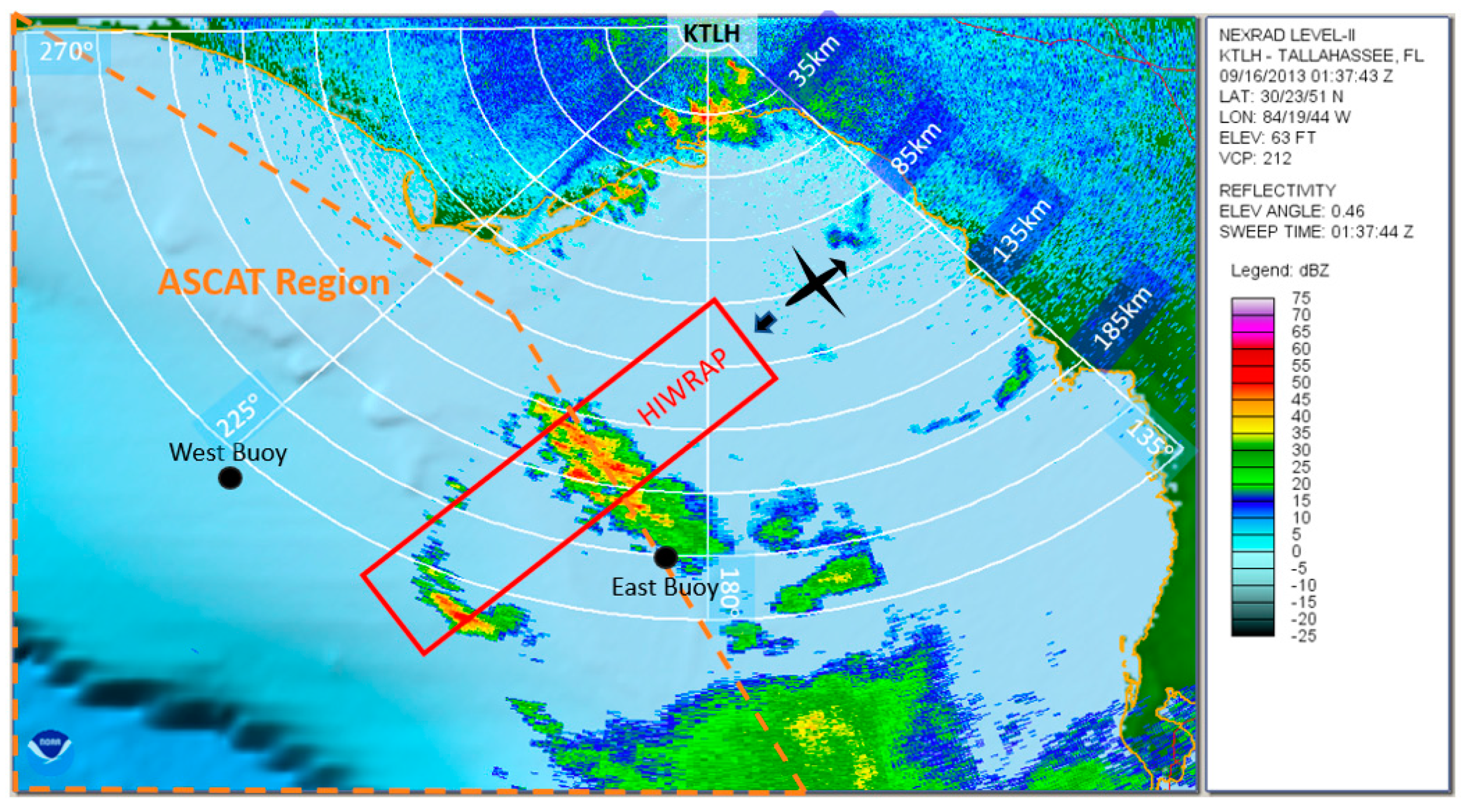
The collocation of the HIWRAP measurement swath for the second GH overpass is shown, in relation to the rain squall line, in Figure 1. This figure presents a range–azimuth display from the NEXRAD Tallahassee radar (KTLH), where range is given in km, azimuth is degrees from north, and radar reflectivity in logarithmic units of dBZ. For example, 25 dBZ (dark green) corresponds to light rain (1 ) and 50 dBZ (bright red) corresponds to heavy rain (64 ). Also shown are the locations of the NOAA ocean buoys to the east and the west of the rain event (black circles) and the region of the satellite ASCAT ocean vector wind measurements (orange dashed lines). The individual remote sensing datasets (NEXRAD and ASCAT) were near-simultaneous and provided overlapping spatial coverage, and the in situ buoy measurements provided ocean surface wind speed (WS) and wind direction (WD) time series that span the HIWRAP observation period.
Previously, results were reported for the TBRE concerning another GH remote sensor named the Hurricane Imaging Radiometer (HIRAD) that used NEXRAD rain measurements for calibration [3]. This present work significantly expands the scope of that previous paper by including the HIWRAP remote sensor and by focusing on the validation of the HIWRAP geophysical retrievals of rain rate and wind speed.
Section 2 provides a description of the HIWRAP instrument, and describes the procedures for the in-flight radar calibration, and geophysical retrieval algorithms of rain rate and wind speed. In Section 3, results are presented of the comparison of HIWRAP wind speed and direction retrievals with independent estimates from collocated satellite and ground-based observations. Finally, Section 4 summarizes the paper and discusses future related research efforts. Additionally, two appendices are included that describe: the airborne HIWRAP radar reflectivity calibration in Appendix A.1 (Appendix A), the SFR3 rain rate retrieval algorithm (Appendix A.2), and the geometric model used for spatial collocation of NEXRAD and HIWRAP 3-dimensional rain measurements (Appendix B).
2. HIWRAP Measurements, Calibration and Geophysical Retrieval Algorithms
2.1. HIWRAP Instrument
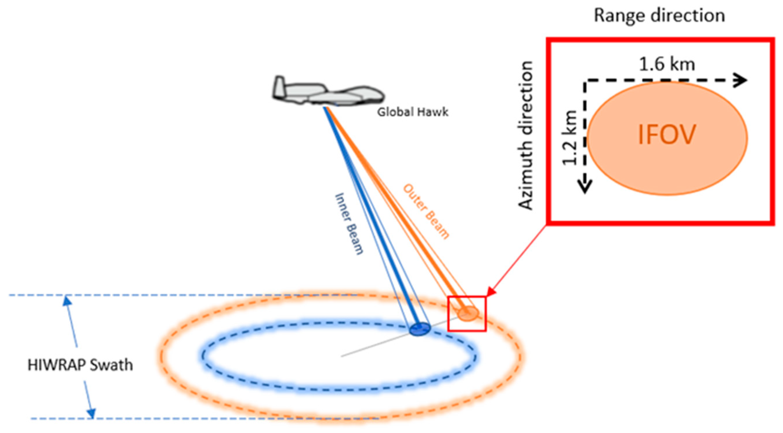
HIWRAP is a dual-frequency radar that measures the 3D structure of atmospheric precipitation backscatter, Doppler frequency, and ocean surface radar backscatter [7]. The antenna is a rotating parabolic reflector, with two offset feeds that produce a horizontally polarized inner beam with a cone angle of 30° and a vertically polarized outer beam at 40° that are both circular in cross-section. During the TBRE, the radar reflectivity is obtained in 75 m RGs from the aircraft to the surface of the earth at a particular azimuth scan angle over the full 360° rotation, for the inner and outer beams, respectively, as illustrated in Figure 2. With the Global Hawk operating at an altitude of 17.5 km, the corresponding HIWRAP measurement swath, for the second GH overpass of the TBRE area, is 27 km (cross-track) by 187 km (along track).
By processing HIWRAP backscatter measurements from multiple azimuth-looks within a conical scan, vertical profiles of rain rate and atmospheric wind (in rain), and ocean surface wind vector are derived. For this paper, only the rain rate and surface wind measurements are addressed.
The radar measurements are geolocated using an ellipsoid earth geometry model that produces longitude, latitude, and altitude for each range gate (RG). The accuracy of this geolocation was verified using HIWRAP radar reflectivity images of land/water boundaries that occurred during a fly-over of the northern Florida peninsula. By comparing the locations of major lakes and rivers with Google Earth maps [8], it was shown that they agreed within <0.5 km (better than half of the antenna Instantaneous Field of View (IFOV) on the surface). Moreover, according to [9], the uncertainty of the corresponding Google Earth 3D terrain model is <7 m for the horizontal and <3 m for the vertical positional accuracy.
2.2. Data Processing
2.2.1. Radar Calibration
Because the HIWRAP dataset provides the average received radio frequency (RF) power measurement in relative power (dB) units, it is necessary to perform an in-flight radar system calibration for this study. The basis of this calibration involves the measurement the ocean surface normalized radar cross-section (), which is defined as the reflected RF energy per unit area of the ocean surface, and this ocean calibration procedure is described in Appendix A.1.
2.2.2. Rain Rate Retrieval
With the HIWRAP radar return (echo) power calibrated, the rain reflectivity is calculated through an iterative single-frequency technique (SFR3), as described in Appendix A.2. Because HIWRAP operates at Ku-band frequency, there is an associated path integrated attenuation (PIA) that must be corrected before the rain reflectivity (Z), in a given RG, can be calculated. Once the PIA-adjusted rain reflectivity is known, then the rain rate is estimated using a Z–R relationship, which is an empirical rain backscatter reflectivity to rain rate relationship based on raindrop-size distribution (rain type classification).
The rain reflectivity Z is similar to the ocean surface , but now applied to the volume backscatter of rain per unit RG volume in units . Using the calibrated, PIA-adjusted, average received power at the input of the receiver , the radar reflectivity factor Z is calculated using the Probert–Jones equation [10].
where r is the range in meters, and the radar factor is
where Pt is the transmit power (Watts), G0 is the antenna peak gain (power ratio), is the pulse volume length (m), is the wavelength (m), and are the antenna pattern half power beamwidths (radians) in the elevation and azimuthal planes, 1024ln(2) is a constant used in approximating the volume, 1018 is the conversion factor between to , and |K|2 = 0.93 is the complex index of refraction for liquid water.
The reflectivity is then converted to rain rate using a Z–R relationship of the form Z = aRb, where R is the rain rate in , and the values of the “a” and “b” coefficients are estimated based on the type of precipitation. Using the calculated reflectivity, the rain rate is then calculated for HIWRAP using Z = 340.56R1.52 from [11], and for NEXRAD using Z = 300R1.4, which is the default from the NEXRAD meteorological handbook [5].
In each RG, the measured radar return power suffers from the extinction by the rain along the propagation path; therefore, it is necessary to correct the measured for the PIA before retrieving the rain rate. The radar frequency-dependent rain extinction coefficient for the nth range gate (kn) is calculated according to Ulaby and Long [12] as:
where the subscript n denotes the range gate number, is the path attenuation in , Rn is the unknown rain rate in , the coefficient kl is 0.0246 for the inner beam frequency (0.0227 for outer beam) and the exponent b is 1.1485 for the inner beam frequency (1.1515 for outer beam). Thus, by calculating the attenuation for each RG, the PIA, is found as the sum of the two-way path attenuations in dB, as
However, since the rain rate of the RGs is not known, the single-frequency rain rate retrieval algorithm is presented in Appendix A.2, where the precipitation return power and PIAs are iteratively solved along the propagation path.
2.2.3. HIWRAP OVW Retrievals
Because the ocean increases monotonically with increasing ocean surface wind speed, it is possible to use radar backscatter measurements to remotely sense this geophysical parameter. Further, because is anisotropic with wind direction, it is also possible to infer WD from radar backscatter measurements obtained at multiple azimuth angles that is provided by HIWRAP’s conical-scanning antenna geometry. Thus, HIWRAP measurements are processed using a maximum likelihood estimation (MLE) technique [13] to infer the “best estimate” wind vector that produced the measured .
This OVW retrieval algorithm is a three-step process, namely (1) collocating multiple “clear-sky” backscatter measurements (from different antenna scans) into cross-track “boxes” on the ocean surface called wind vector cells (WVC), (2) evaluating a cost function to find possible combinations of WS and WD that minimizes the square difference between measured and modeled , and (3) selecting the best WD from multiple possible wind direction solutions (aliases).
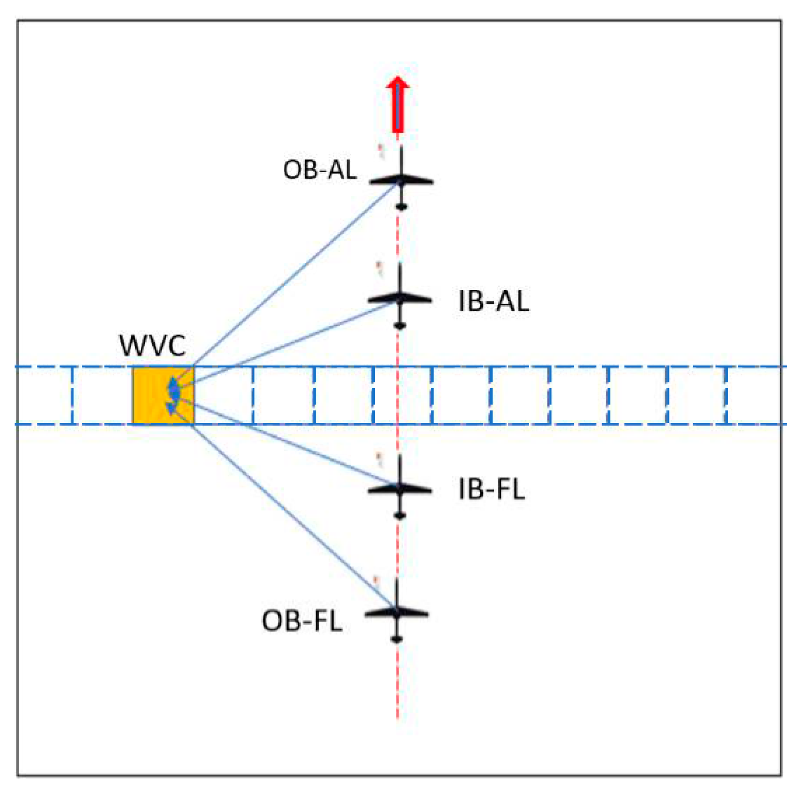
During the GH flight, the conical scanning HIWRAP inner and outer beams view a cross-track grid of WVCs as illustrated in Figure 3, which results in each having 4 different azimuth looks at the same 4 × 4 km box. For example, for a given antenna beam, the azimuth difference between fore and aft-looks varies with the cross-track position of the WVC, which results in delta-azimuth angles from 180° (along the aircraft track) to 0° (at the edge of scan). Given that multiple antenna scans lie within a selected WVC, this produces many measurements (typically 40–60), which are inputs to the OVW retrieval algorithm.
For the OVW retrieval, we use both the measured and modeled to evaluate a cost function. The measured is calculated using the calibrated measured power in the surface RG from the HIWRAP data (see Appendix A.1.1). The theoretical (modeled) is obtained using the NSCAT-1 Geophysical Model Function (GMF), an empirical relationship, derived from the NASA scatterometer (NSCAT) [14] as
where is a function of frequency f, electromagnetic polarization pol, EIA, and radar azimuth look direction Az, and of the geophysical variables WS and WD. Further, note that is anisotropic with the relative-WD, which is defined as the difference between WD and the radar Az look direction.
To retrieve wind vector, the cost is parametrically evaluated, where the measured and the radar variables f, pol, EIA, and Az are inputs, and the WS and WD are unknown.
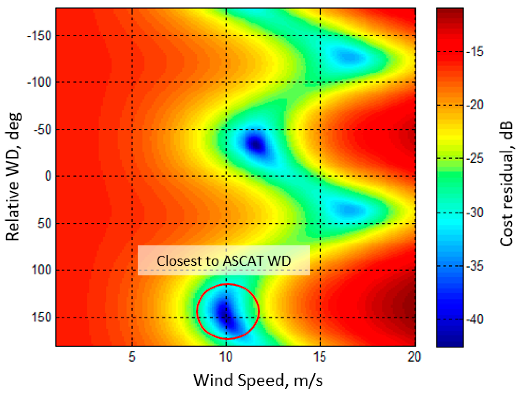
Figure 4 shows an example of the cost surface, which is the MLE residual that is plotted in dB for the selected WVC in Figure 3. The X and Y axes are, respectively, the “trial” WS and WD that are evaluated, and the solutions are the local minima of the cost surface. For this case, there are four local minima plotted in various shades of blue, which represent possible wind vector solutions (aliases). The depth of the null is an indicator of the likelihood (probability of the correct solution); but all are reasonable possibilities to produce the collection of measurements. While the choice of the best solution is beyond the scope of this paper, algorithms exist within the OVW science community, which achieve >90% success in selecting the correct solution [15]. Regardless, for this paper, the WD closest to the ASCAT WD product is selected.
3. HIWRAP Geophysical Retrieval Validation
3.1. Collocated Measurements
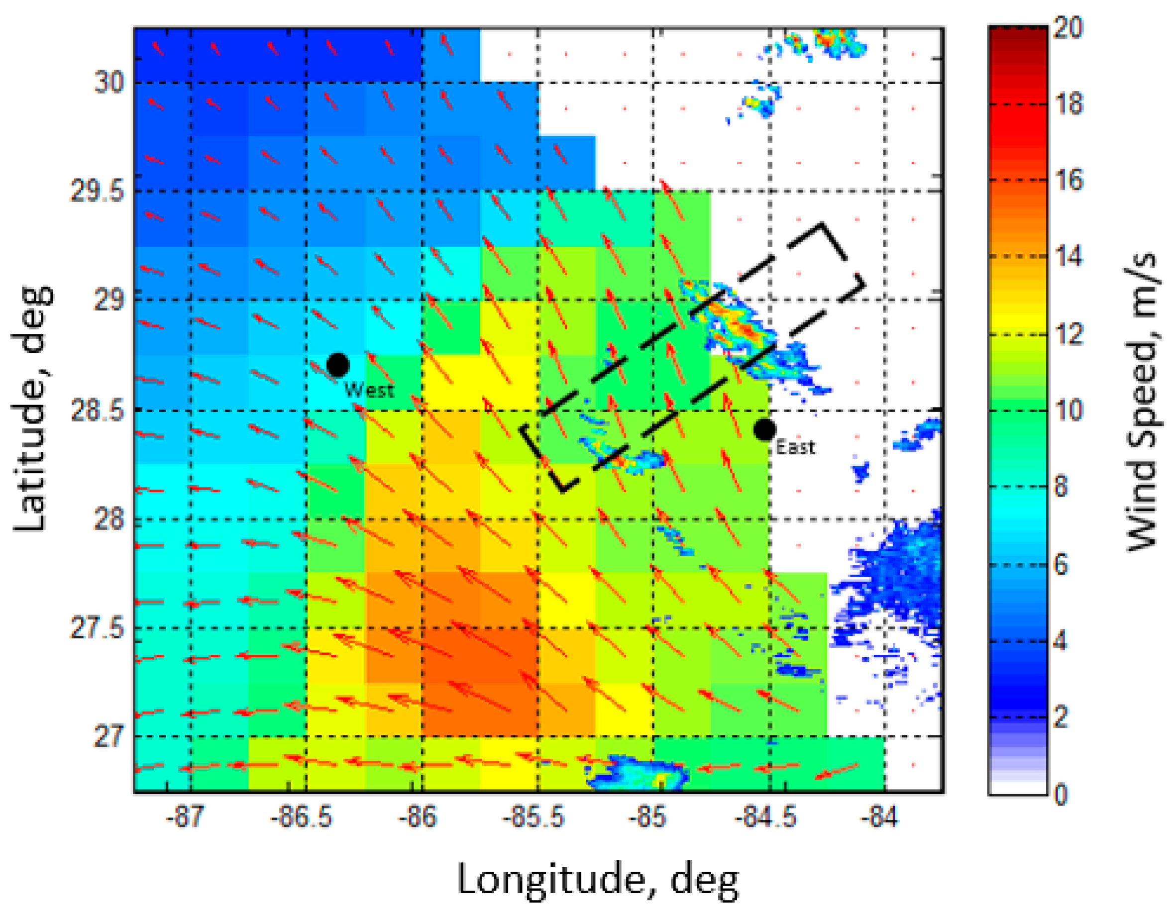
The HIWRAP geophysical retrievals (ocean vector wind and rain rate) are validated against independent estimates. For OVW, there are two sources, namely the ASCAT OVW product and in situ anemometer recordings from two NOAA ocean buoys. The region of intercomparison was the HIWRAP swath (second GH pass over the squall line), which was a rectangular region 27 km × 187 km. A composite image of the independent sources of geophysical estimates is given in Figure 5, where near-simultaneous ASCAT and NEXRAD measurements are presented, with the squall line located at 28.8 N × 84.6 W at the time of the GH overflight.
3.2. HIWRAP Ocean Wind Vector Validation
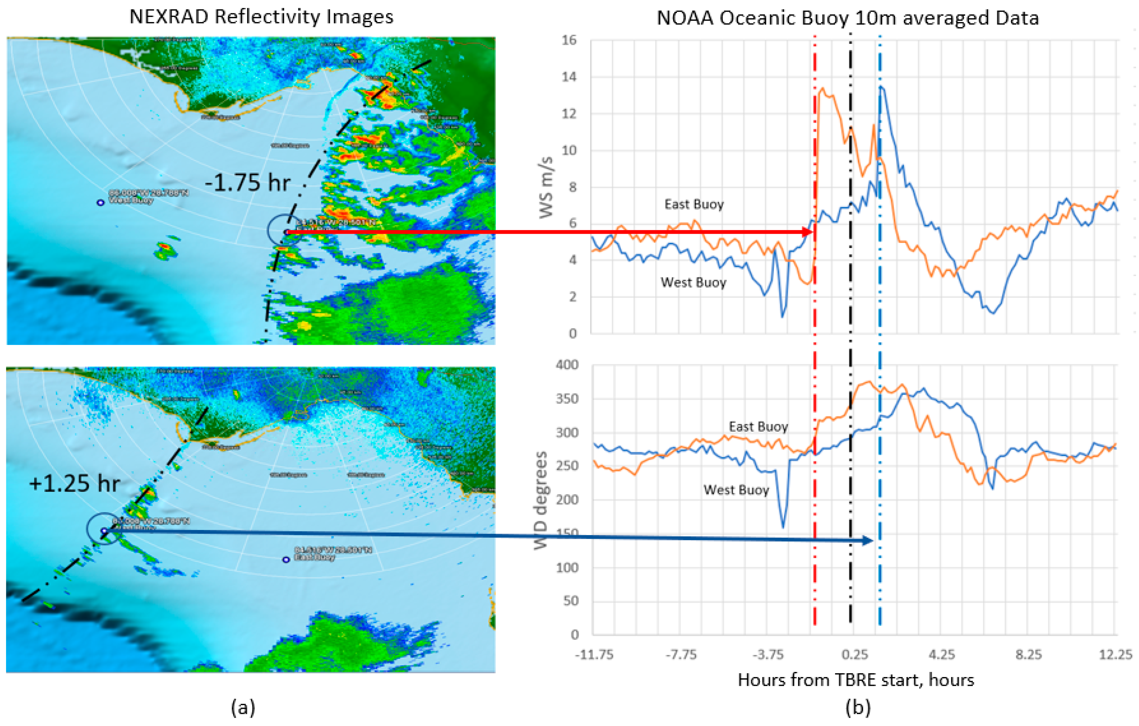
As shown in Figure 5, the wind field from ASCAT is fairly uniform at 10–11 over the HIWRAP swath except that there are no measurements at the beginning (upper portion). On the other hand, the ocean buoy anemometer measurements are very effective in capturing the timeseries of WS and WD, associated with the passage of the propagating atmospheric weather front and squall line. This is illustrated in Figure 6 (right panels), where the timeseries of WS and WD are displayed for the East (orange) and West (blue) buoys that are separated by ~180 km. Also shown (left panels) are the corresponding NEXRAD radar reflectivity images (dBZ), which illustrate the leading edge of the weather front arrival, at the respective buoy locations. The East buoy sees the frontal passage ~1.75 h before GH overpass time (red dashed line in panel b), and the arrival time at the West buoy is ~3 h later (blue dashed line in panel b).
For the East buoy, the passage of the weather front is characterized by a rapid increase in WS (of 8 ) and an associated change in wind direction (by 40°). By the time that the weather front reached the West buoy, its intensity is diminished and the change in WS (of 5 ) is less, as is the change in WD (by 15°). Using these data, the average propagation speed for the squall line is estimated to be ~17
As previously mentioned, the aerial extent of HIWRAP wind measurements was relatively small, and the resulting number of collocated comparisons does not provide a sufficient population for a robust statistical analysis, although evaluation of these independent measurements suggests high-quality HIWRAP retrievals. Figure 7 shows a gridded plot of ASCAT 25 km OVW, with the corresponding 12.5 km gridded retrievals from HIWRAP that selects the closest HIWRAP WD alias to the ASCAT WD. Over this lower 2/3rd of the HIWRAP swath, both the HIWRAP and ASCAT OVWs are in good agreement. Over this region, the average ASCAT OVW is 10.5 at 157° and HIWRAP is 11.6 at 144°, which is well within the accepted OVW measurement requirement of WS ≤ ±2 and WD ≤ ±20°. Further, it appears that HIWRAP vectors show spatial changes that are not captured in the coarser-spatial-resolution ASCAT results.
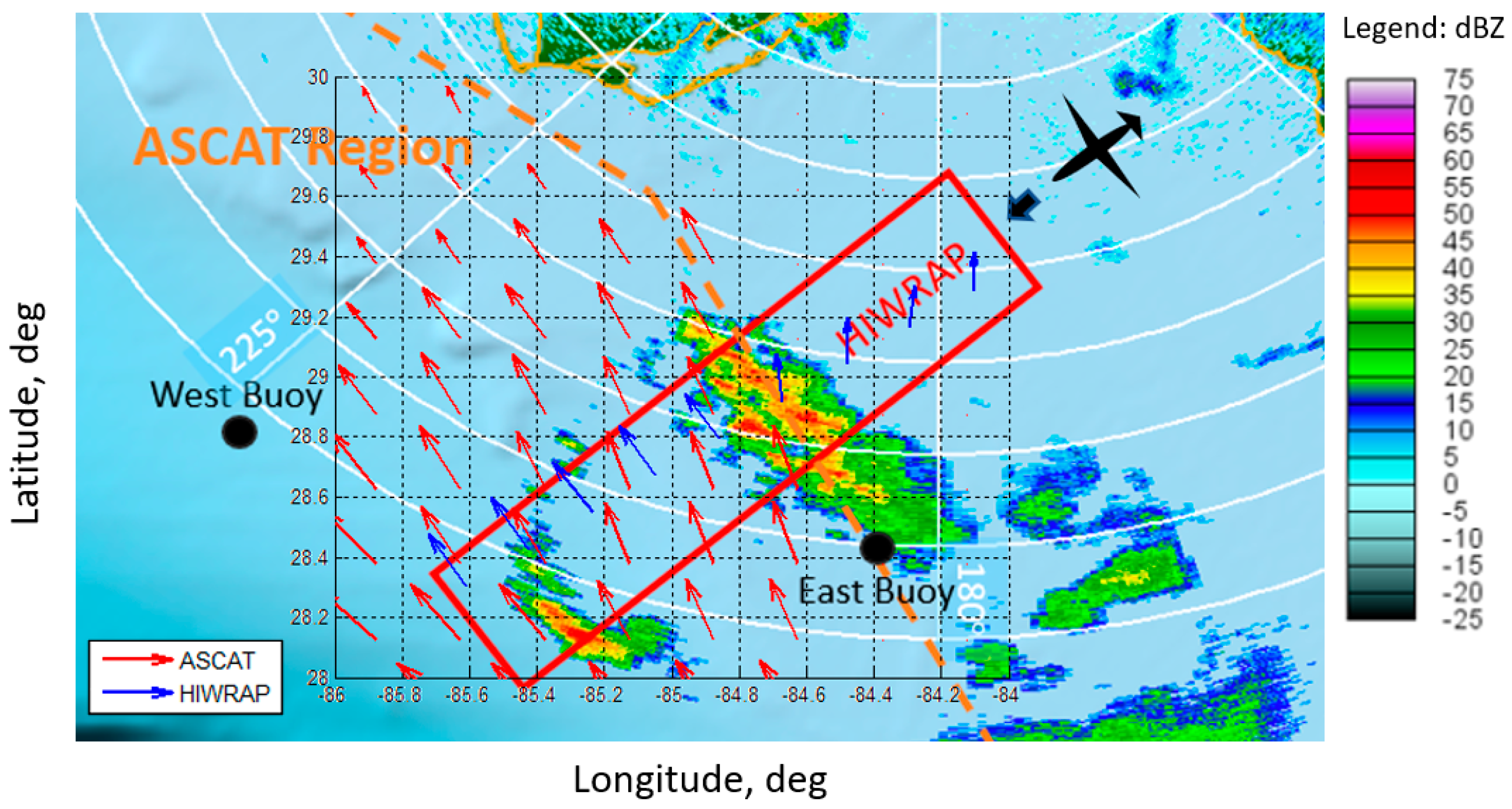
Next, concerning the upper 1/3rd of the HIWRAP swath (Figure 7, longitude 84.6 W to 84.0 W), there is an abrupt reduction in the WS (~4.7 ) and a rapid clockwise rotation of the WD by (~28°). To better understand the realism of this change, the NEXRAD rain reflectivity image (dBZ) is superimposed onto the ASCAT and HIWRAP wind vector plot in Figure 8. The rapid changes in OVW occurs precisely at the location of the weather front, which suggests that HIWRAP captures the true change in the surface wind that is consistent with the buoy anemometer timeseries. Moreover, it appears that HIWRAP-retrieved wind vectors are present within the rain cells located at 28.8° N × 84.8° W and 28.3° N × 85.4° W, which also agree with ASCAT.
This is important because ASCAT operates at C-band, which is much less affected by rain than is HIWRAP Ku-band. However, since, the HIWRAP measures rain reflectivity in the atmosphere, it provides excellent quality control to remove rain contaminated surface echo powers, which historically have caused seriously degraded Ku-band OVW retrievals [16]. For these results, a conservative approach was adopted to make a binary decision to delete all with rain attenuation. For future hurricane observations, where strong winds and rain cannot be spatially separated, a less conservative approach would be to develop a rain attenuation correction for less severely contaminated surface RG samples, which is the basis of future proposed research.
3.3. HIWRAP Rain Rate Validation
Using the HIWRAP-calibrated return power in RGs (Appendix A.1), the rain reflectivity Z is calculated through an iterative single-frequency technique (Appendix A.2) that involves estimating the PIA to correct the rain reflectivity, and then the rain rate is calculated using a Z–R relationship. Therefore, HIWRAP rain rate validation implicitly involves PIA validation, which unfortunately cannot be independently evaluated with the available NEXRAD data. As a result, the basis of HIWRAP rain rate validation is the comparison of independent, simultaneous, and collocated NEXRAD rain rate measurements. Fortunately, within the radar meteorology community, the NEXRAD rain rate product is an acceptable standard; however, even with this, there are several caveats (uncertainties) that limit the HIWRAP rain measurement validation. As a result, the following are important factors that must be considered in this process.
First, because of the differences in the radar operating frequencies (Ku-band for HIWRAP and S-band for NEXRAD), there are different Z–R relationships, which are empirically derived for several categories of rain type (assumed raindrop-size distributions). For this comparison, the Z–R relationships described in Section 2.2.2 are used. Second, differences in the measurement geometry must be considered. For example, HIWRAP measures from the top of the atmosphere downward at a high grazing angle (50–60°), while the NEXRAD geometry is along a nearly horizontal path. However, to make valid rain rate comparisons, the NEXRAD and HIWRAP atmospheric sampling volumes must be simultaneous and equal.
So, to satisfy the requirement for simultaneous measurements, it is reasonable to assume that on the time scale of a few minutes, the vertical distribution of rain is spatially frozen in altitude, while the entire rain event is advected horizontally by the motion of the propagating weather front. So, sequential NEXRAD rain rate measurements, at different altitude levels, are aligned in time to remove collocation errors associated with the rain advection and dynamic changes in the rain feature that may occur during the ~5 min sampling interval. To accomplish this, we use a morphing technique [17] to provide time-interpolated rain images at 1 min intervals that results in an acceptable 3D alignment of the rain features with an uncertainty of <±30 s or <±500 m. Further, since the HIWRAP conical scan samples the 2 km cubes at different times, the collocation time is based upon the average HIWRAP sampling time, where forward and aft-looks and inner and outer beam are separated into four different rain retrieval cases.
To ensure equal sampling volumes, NEXRAD rain rate measurements are interpolated to the HIWRAP RGs using the NEXRAD Spatial Interpolator that is described in Appendix B. These collocated rain rate measurements are then binned and averaged over the many RGs and antenna scans into a common 2 km cube of rain volume that approximates the spatial resolution of NEXRAD.
Finally, because of expected radar calibration differences and of uncertainties in the assumed Z–R relationships, there could be large rain rate differences between two collocated HIWRAP and NEXRAD rain estimates. Therefore, rather than comparing differences, the preferred metric used is the ratio of collocated rain rates (RH/RN), where RH is the HIWRAP rain rate and RN is the corresponding NEXRAD.
On the other hand, we believe that the spatial distribution of relative rain rate is the strongest validation metric. If there is good spatial and temporal collocation of the two radar measurements, then high correlation of the two rain rate images is strong evidence that both radars are performing well.
3.3.1. HIWRAP and NEXRAD Rain Rate Comparisons at Low Resolution
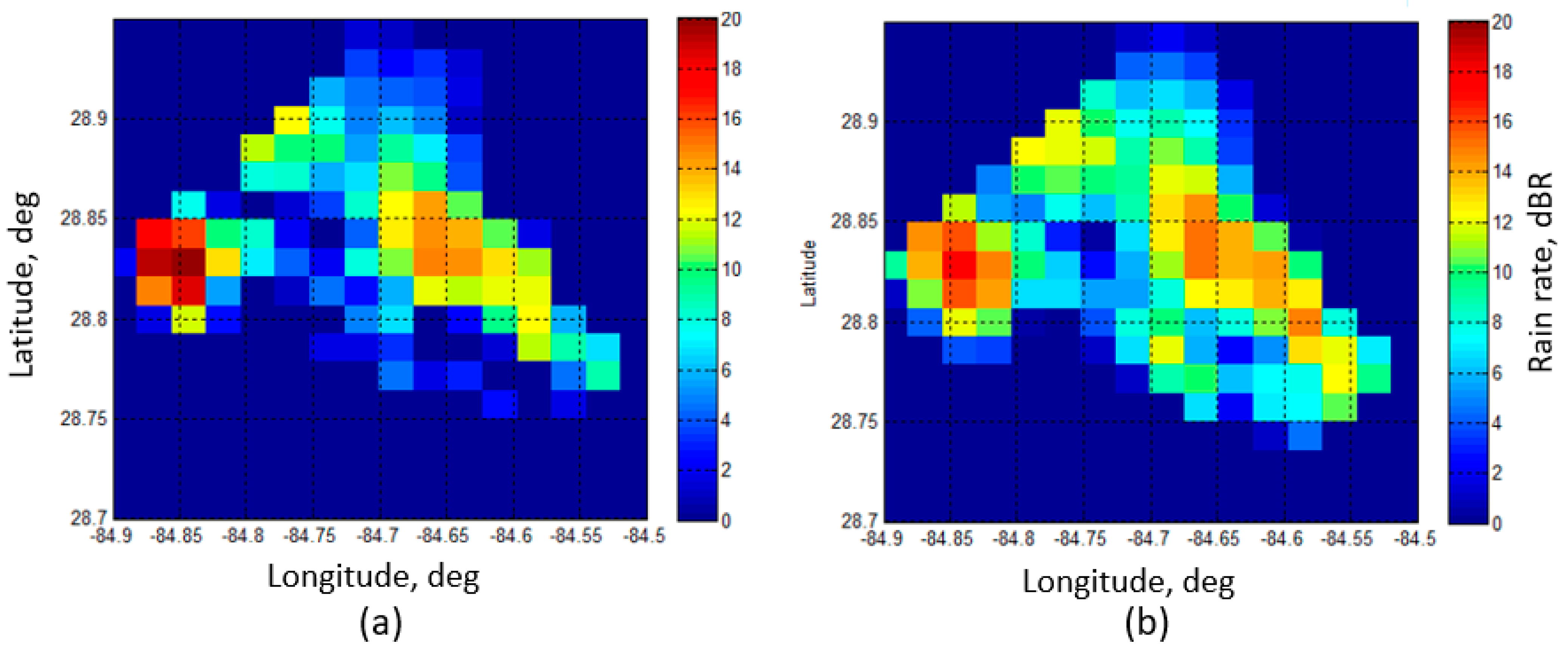
First, consider a comparison of HIWRAP and NEXRAD rain rates at the NEXRAD spatial resolution (2 km cubes) and the lowest elevation L-1 scan (4 km altitude), as shown in Figure 9. These are Constant-Altitude Plan Position Indicator (CAPPI) images of the rain squall line for HIWRAP (panel a) and NEXRAD (panel b) that occurred at the beginning of the GH flight. These CAPPIs were produced using binned averaged HIWRAP-retrieved rain rates (for the inner and outer beams over all azimuth angles combined) and interpolated NEXRAD rain rates to common 2 km cubes. Rain rates are displayed in logarithmetic units of dBR , where 0 dBR corresponds to 1 and 20 dBR corresponds to 100 of rain.
The spatial distribution of the precipitation features in these two CAPPIs are in remarkable agreement, and the 2D normalized cross-correlation coefficient is 89%, with zero lag in both longitude and latitude directions. We conclude that this comparison supports the validity of the HIWRAP rain retrieval.
Next, the statistical results of the comparison of HIWRAP and NEXRAD rain rates (>1 mm h−1 in Figure 9), are presented in Table 1. There are four different sub-categories for HIWRAP rain retrievals (combinations of inner and outer beams and fore and aft-looks), and within each, there are three statistical metrics, namely, average of HIWRAP rain rates, average of NEXRAD rain rates, and averages of rain rate ratios (RH/RN).
First, consider the comparisons between forward and aft-looks for a given beam. For both beams, the statistics are nearly identical, even though the time difference between these CAPPIs is ~2 min. During this interval, the rain event has propagated slightly more than 2 km, and a different NEXRAD time-interpolated (morphed) image is used for the comparisons; yet the results are the nearly the same. We believe that this is the result of the fidelity of the HIWRAP/NEXRAD collocation that results from the use of the NEXRAD Spatial Interpolator model. Further, this is strong evidence that supports the validity of the HIWRAP rain rate retrievals. On the other hand, there are small differences in the statistics for the inner and outer beams, e.g., RH/RN = 0.84 for inner beam and equal 0.63 for outer beam. This minor difference could be related to the geometry differences and possibly in the radar calibration, which will be investigated in future work.
3.3.2. HIWRAP and NEXRAD Rain Rate Comparisons at High Resolution
Next, the validation of HIWRAP measurement of vertical profiles of rain rate is presented, and for this analysis, it is necessary to increase the rain rate spatial sampling resolution to 500 m. For HIWRAP, the native rain rate sampling occurs in 75 m RGs, which is 3× better than the Nyquist spatial sampling requirement. Within a 500 m cube, individual RG volumes are stacked cylinders with the axis oriented vertically with heights of 75 m (vertical) and radii of 500 m (horizontal). Thus, HIWRAP measurement geometry gives excellent vertical rain rate profiling with modest horizontal spatial averaging.
On the other hand, the NEXRAD RG volume are also short cylinders, but now the orientation of the cylinder axis is horizontal, with the cylinder height (horizontal range dimension) of 250 m and a cylinder radius of 800 m (altitude dimension). This poor vertical resolution does not satisfy Nyquist spatial sampling, and the resulting vertical rain rate profile is significantly aliased.
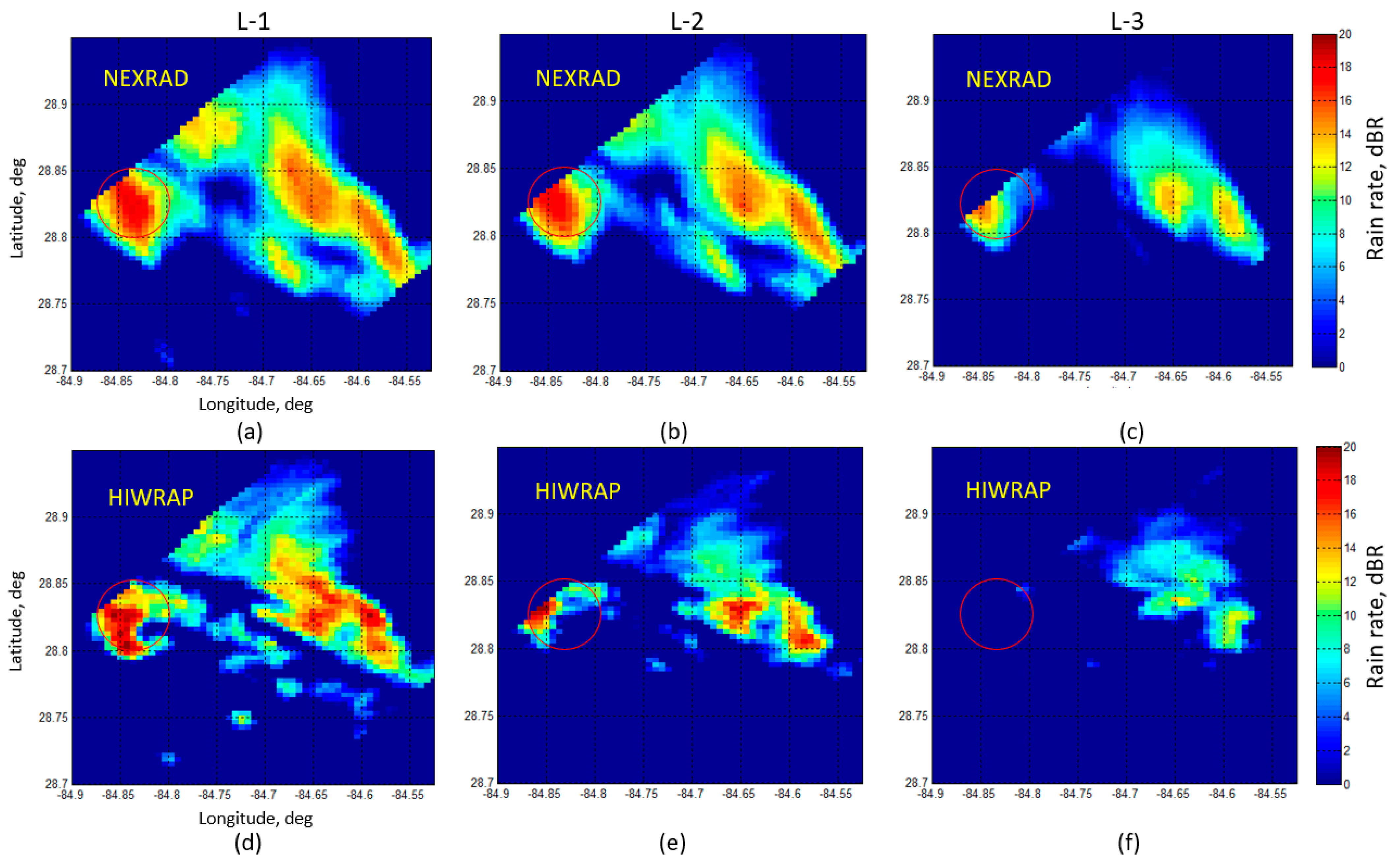
Collocated HIWRAP and NEXRAD rain rates are binned and averaged into 500 m cubes and are displayed in Figure 10 in three CAPPI plots of increasing altitude at NEXRAD L-1 (3.5 km), L-2 (4.5 km), and L-3 (6 km). In the NEXRAD images, the aliasing of the rain rate vertical profile with increasing altitude is quite evident, which causes precipitation to be present in L-2 and L-3, where the corresponding pixels for HIWRAP have little to no rain. This is especially visible in the heavy rain pattern at 28.825 N × 84.84 W (in the red circle). For example, in the L-3 CAPPI there is no rain detected by HIWRAP, while NEXRAD measures 14 dBR (25 ). On the other hand, for the L-1 images, both are highly correlated, but the HIWRAP image has more realistic small-scale rain structure variability.
The final HIWRAP rain rate comparison deals with vertical profile measurements. Consider 2D images of rain rate vertical profiles given in Figure 11 that are produced using the line-of-sight geometry for the HIWRAP outer beam looking aft along the aircraft ground track (dash-red line). The left image (panel a) is the HIWRAP binned average rain rate vertical profile in 500 m cubes, and the center image (panel b) is a simulated rain rate vertical profile using the HIWRAP measurement (panel a) and convolving with the antenna pattern of NEXRAD. Finally, the right image (panel c) is the corresponding NEXRAD measurements collocated with HIWRAP 500 m cubes. Note that the sloping red lines represent the height of L-1 to L-3 as the radar range increases from left to right. This image is the result of interpolation of NEXRAD measurements from the entire volume scan, except for the lower portion, which is an extrapolation of L-1 measurements to the surface. These images are all quite similar, exhibiting high correlation in the spatial distribution of rain rate, and the major difference between them is small-scale rain structure in the higher-resolution HIWRAP image (panel a), which is examined further in Figure 12.
Considering the HIWRAP rain rate profile image (Figure 11a), it is important to determine whether or not the small-scale rain structure is a geophysical signal or rain rate retrieval error. To investigate this, consider Figure 12, where the left image (panel a) is the same HIWRAP aft looking outer beam vertical profile, with a single beam location indicated by the magenta line of sight. The right panel b is the corresponding series of radar parameters plotted against the RG number (inversely proportional to altitude) for the selected single radar profile.
In panel b, the solid green curve is the raw rain reflectivity (dBZ) that is processed to simultaneously retrieve the PIA (dashed magenta curve), the PIA corrected reflectivity (dashed-black curve), and the rain rate (solid red curve). Also shown is the corresponding NEXRAD-interpolated rain rate (solid blue curve). Next, consider the rain rate vertical profile (red curve), which places the top of the intense rain at ~5.3 km (RG = 210), and over the next 15 RGs, there are two peaks of rain follow the raw reflectivity. Because the PIA is low, there is high confidence that HIWRAP accurately captures this small-scale structure of the rain rate profile, which is plausible given the heterogeneous nature of rain.
Next, over the next 40 RGs, there is a significant drop in reflectivity followed by two peaks in raw reflectivity. Here, the PIA increases from 5 to 10 dB, but the retrieved rain rate also appears plausible. So, we conclude that the HIWRAP-retrieved rain rate is profiling the small-scale structure of the rain cells. Similar scenarios were examined for many profiles with the same conclusion that the HIWRAP rain rates are a reasonable estimate.
Given this conclusion, how does one justify the NEXRAD rain rate profiles? The answer is the effect of the poor vertical resolution of the antenna beam, which is ~1.6 km. When examining the CAPPIs in Figure 10, it is apparent that the NEXRAD rain rates are aliased too high for the altitude range L-1 (3.5 km) through L-3 (6 km). Thus, the NEXRAD antenna pattern acts as a low pass filter, which smooths the rain rate vertical profile and extends rain into the higher altitudes. To support this hypothesis, consider Figure 11 panel b, where the simulated HIWRAP rain rate image was processed using a Gaussian spatial filter that represented the NEXRAD antenna pattern. After performing this antenna pattern convolution, the resulting simulated HIWRAP image (panel b) is very similar to the measured NEXRAD image (panel c).
4. Discussion
This paper reports the first in-flight radar calibration for HIWRAP to provide calibrated measurements for atmospheric rain and ocean surface roughness. The calibration was accomplished by measuring the normalized ocean radar cross-section and comparing this against modeled values using known geophysical parameters and independent collocated measurements of ocean surface wind speed and direction provided by ASCAT.
The primary goal of this work was to validate the HIWRAP geophysical retrievals of 3D atmospheric rain rate and ocean surface wind vector, which will enable critical hurricane measurements for the NASA Hurricane and Severe Storm Sentinel (HS3) mission. Concerning the HIWRAP rain rate retrieval, this was accomplished through the development of a single-frequency rain rate retrieval (SR3) algorithm.
The HIWRAP SR3 retrievals were validated through near-simultaneous and collocated comparisons of a tropical squall line of convective rain cells with independent 3D rain rate measurements from the National Weather Service’s NEXRAD meteorological radar. While NEXRAD is a reliable standard for measuring rain rate, the NEXRAD geometry for the TBRE was less than ideal for the validation of HIWRAP. When comparing collocated HIWRAP and NEXRAD low-spatial-resolution (2 km) rain measurements in CAPPIs at 4 km altitude, the agreement in the spatial distribution of rain is excellent. Additionally, rain rate magnitude comparisons, of rain between 1 and 100 , at the pixel level are very good. The mean ratio of HIWRAP to NEXRAD rain rates (RH/RN) for four different HIWRAP retrievals (2 beams and fore and aft-looks) ranging between 0.84 (inner beam) and 0.63 (outer beam). On the other hand, when comparing HIWRAP and NEXRAD rain rate vertical profiles at high resolution (500 m), we conclude that HIWRAP rain rate profile measurements are superior to NEXRAD because of the top-down viewing geometry and the excellent RG resolution in altitude.
Also, presented are the results of the validation of HIWRAP retrievals of ocean surface wind speed and direction by comparison with the ASCAT wind measurements and in situ anemometers on two NOAA ocean buoys. From our analysis, we conclude that the HIWRAP retrieves ocean surface wind and rain rates that are consistent with the supporting ground and satellite estimates, thereby providing validation of the geolocation, calibration, and wind vector retrieval algorithms used to infer ocean surface wind vectors. Further, we recognize that HIWRAP can be useful for providing high-resolution information within tropical storms and hurricanes. One key advantage of using HIWRAP as an ocean surface wind scatterometer, is that it is self-calibrating for atmospheric rain attenuation. The ability to detect rain along the propagation path and to correct for the associated signal attenuation, removes a significant source of wind retrieval error for Ku-band scatterometers [16].
Future work includes the in-flight cross-validation of the single-frequency wind and rain rate retrieval algorithms, with the dual-frequency methods described in [18]. Additionally, we plan to perform wind speed and rain rate retrievals for other hurricane flights, where HIWRAP operated. Finally, the TBRE will be revisited one final time to include the Hurricane Imaging Radiometer (HIRAD) wind speed and rain rate retrievals, and conduct validation assessments with HIWRAP, NEXRAD, ASCAT and the NOAA ocean buoy sensors.
Author Contributions
This research is the dissertation topic for J.C. at the University of Central Fl. He is responsible for the various algorithm developments, data processing, and the HIWRAP validation analysis, and he is the corresponding author responsible for the review and editing. W.L.J. is the PhD advisor for J.C. and responsible for technical guidance and review of J.C.’s work; and G.M.H. is the PI for the HIWRAP sensor, who contributed the HIWRAP data, and he provided technical guidance and review of the radar algorithms. All authors have read and agreed to the published version of the manuscript.
Funding
This research received no external funding. HIWRAP data were collected as part of the NASA HS3 mission.
Institutional Review Board Statement
Not applicable.
Informed Consent Statement
Not applicable.
Data Availability Statement
The HIWRAP data are available at https://ghrc.nsstc.nasa.gov/pub/fieldCampaigns/hs3/HIWRAP/doc/HS3_HIWRAP_dataset.pdf (accessed on 17 March 2021). The NEXRAD data are publicly available online through the NOAA National Center for Environmental Information (NCEI) as level 2 data products. The ASCAT data are available from https://www.ospo.noaa.gov/Products/atmosphere/ascat/ (accessed on 17 March 2021). The NOAA buoy data are available from https://www.ndbc.noaa.gov (accessed on 17 March 2021).
Conflicts of Interest
The authors declare no conflict of interest.
Appendix A. HIWRAP Calibration and Rain Retrieval Algorithms
Appendix A.1. Airborne Calibration Using the Ocean Normalized Radar Cross-Section
Appendix A.1.1. Measured Normalized Radar Cross-Section ()
For a single pulse, the ocean surface is calculated from the average measured received power Pr in the surface RG as;
where G is the 2D antenna gain (spherical coordinates), Pt is the transmit power, is the wavelength, is the ocean normalized radar cross-section, T is the round-trip time, r is the range, is the integration period (transmit pulse length), and are spherical coordinates with the Z axis aligned with the line of sight for inner and outer beams, and the differential solid angle is .
Then, the average power for a given range gate (n) is calculated by integrating over the period
For the integral over the antenna pattern, by splitting the solid angle into differential surface elements, a myriad of antenna pencil beams is created where subscripts (i,j) corresponds to the elevation position i and azimuth position j for a given pair, which are evenly spaced in elevation and azimuthal steps. This allows us to transform the integral into the summation of power, and the total returned power is then given as,
where is the integrated reflected transmitted power of a single element (pencil beam) at a specified range gate. Then, solving for the measured ocean , and setting n = s, the surface gate number.
Appendix A.1.2. Calibration
The measured power Pm is the average received power (at the antenna output), which is amplified by the receiver gain and digitized at the receiver output. Since the system gain is unknown, we define the calibration factor C to be the dB offset between the input and output of the receiver,
To calibrate HIWRAP, the and were compared for >20,000 clear-sky surface RGs (uniformly distributed over 360° of azimuth rotation), which were analyzed to find the best estimate of the calibration factor from the observed calibration factor histogram. Experimentally, it was observed that the shape of this histogram was a log-normal distribution, which is Gaussian when calibrating in dB units; therefore, the mean value of the best-fit Gaussian pdf is given by:
where both and are in dB units. This analysis resulted in a C factor of −71.32 dB averaged for inner and outer beams, with a standard deviation of 1.7 dB. It is important to recognize that this factor accounts for the difference in the references for the measured σ o (at the receiver output) and modeled (at the receiver input).
Appendix A.2. Single-Frequency Rain Rate Retrieval (SFR3)
As designed, the HIWRAP operates at two frequencies (Ku-band ~14 GHz and Ka-band ~37 GHz), so that the PIA can be estimated from differential frequency techniques. Unfortunately, for the TBRE the Ka-band channel was not available, so a single-frequency rain rate retrieval (SFR3) technique was developed, which uses an iterative technique to simultaneously calculate the rain and the PIA sequentially along the range gates of the HIWRAP beams. This technique is an expansion on the Hitschfeld–Bordan (HB) method [19], which iteratively calculates the rain and PIA. Although simple, the (HB) method is inherently unstable, and it requires constraints to prevent divergent solutions due to an exponential runaway of overestimating rains, caused by measurement noise and a lack of knowing the true Z–R relationship.
To mitigate this, other techniques such as surface reference methods described by Iguchi and Meneghini in [19] are applied, which use the peak value of the surface echo to estimate the PIA along the slant path. Although this method can be effective, it is unable to retrieve rain when the surface echo is contaminated by rain. Thus, the SFR3 method provides a method of retrieving rain, without prior knowledge of the PIA along the path, by apply the HB method with an iterative divergence correction constraint.
So, using Equation (4), R and PIA can be calculated iteratively by RG location. The procedure begins by solving for R1 (using the default Z–R relationship with the a = 340.56 and b = 1.52 from [11]) and then using the iterative equation below to solve for the PIA.
This procedure is repeated iteratively until the threshold altitude of 1.25 km, where the received power is contaminated by the surface echo. Thus, lower than this altitude no retrieval is possible.
Divergence Mitigation through Z–R Correction
According to Maki et al. [20], the “a-coefficient”, in the Z–R relationship for a tropical squall line, increases with rain intensity and atmospheric temperature, while the “b-coefficient” remains relatively constant. Since divergence of the SFR3 algorithm occurs only in high intensity rain, it is reasonable to assume that the a-coefficient is larger, and a simple method to compensate for this is to incrementally increase the a-coefficient used by a small step size , until the series converges (by checking the maximum allowable PIA and R limits):
Once the series converges, it most likely overestimates the rain. To mitigate this, the a-coefficient is increased by a sizeable value , which drives the results toward the true solution. Thus, the final a-coefficient is:
Although somewhat ad hoc, the divergence mitigation technique is quite effective, since increasing the a-coefficient beyond the true value only marginally underestimates the rain.
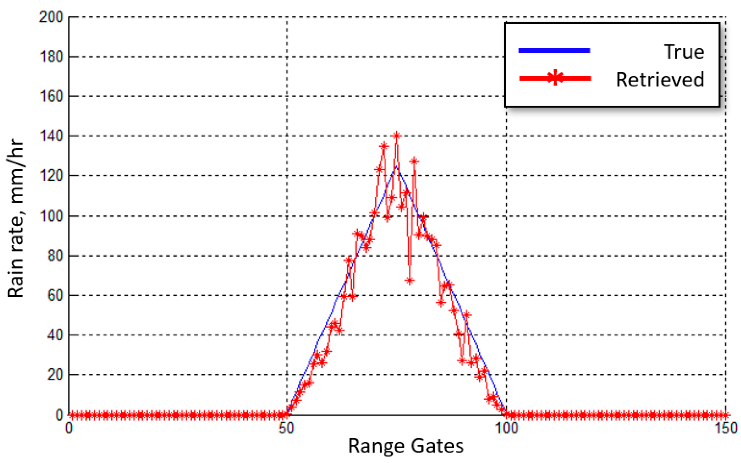
This SFR3 algorithm was developed and evaluated in a Monte Carlo simulation in to tune the algorithm and analyze how the algorithm performed under high rain. The Z–R coefficients were fixed (a = 440.56 and b = 1.52) for three cases with an assumed triangular rain rate profile with a maximum rain rate of 100, 125, and 150 (based on the maximum NEXRAD rain rate for the TBRE of ~108 ). During testing, 100 trials of simulated Pr measurements were perturbed by Gaussian measurement noise of 1 dB std. Using the simulated backscattered power in RGs, the SFR3 algorithm was run by setting the max threshold values (maxR = 150 and maxPIA = 30 dB) and a-coefficient increments ( = 2 and = 50). The root-mean-square rain rate error for the 3 simulation cases were, respectively, 3.24, 3.41, and −8.67 , which corresponded to a percent error of 17.2%, −13.0%, and −36.6% from the modeled rains. An example of a single trial of the retrieval for the 125 case can be seen in Figure A1, where the triangle function rain profile is simulated in blue, and the SFR3-retrieved rains are in red.
Figure A1.
Simulated triangular rain profile with a maximum rain at 125 . The blue is the simulated rain profile, while the red is the retrieved rain rates using the SFR3 algorithm (single random noise trial).
Figure A1.
Simulated triangular rain profile with a maximum rain at 125 . The blue is the simulated rain profile, while the red is the retrieved rain rates using the SFR3 algorithm (single random noise trial).

Appendix B. NEXRAD Spatial Interpolator
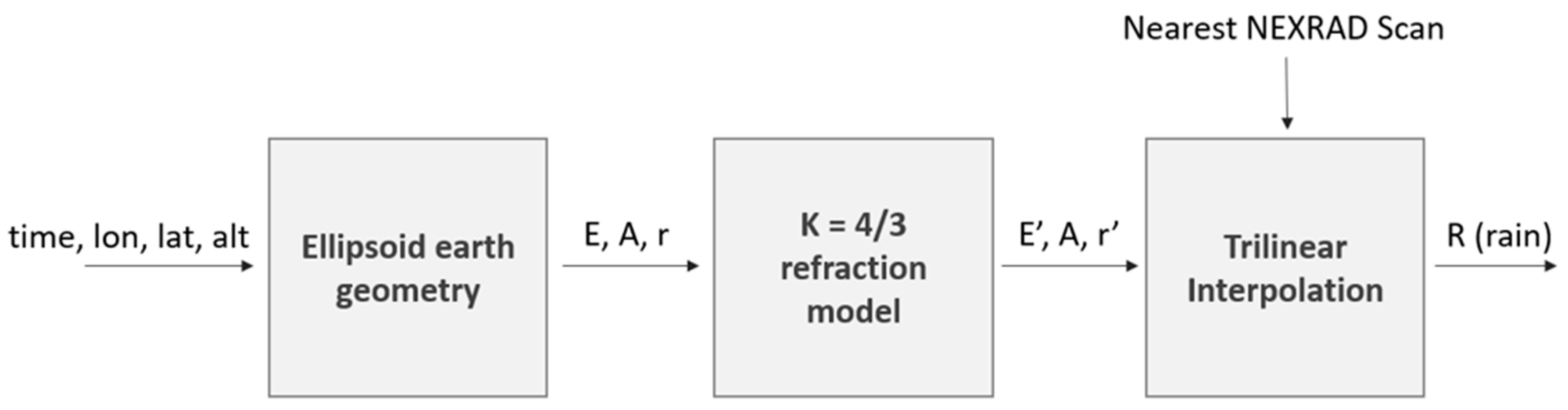
This appendix describes the NEXRAD Spatial Interpolator, which uses temporally aligned NEXRAD data to produce interpolated rain rates, given an input longitude, latitude, and altitude. This method is outlined in Figure A2, where HIWRAP data are first geolocated to the spherical reference frame of NEXRAD using ellipsoid earth geometry. These coordinates are in the line of sight (LoS) of the NEXRAD radar, where the NEXRAD measurements are refracted through the atmosphere, causing an arced path. This is accounted for using a k = 4/3 refraction model, where the change in elevation and range due to the refraction are calculated. With the input coordinates converted to NEXRAD’s refractive spherical coordinate system, the closest temporally aligned NEXRAD dataset in time is selected, where a trilinear interpolation of rain is performed using the nearest eight surrounding points to the input coordinate.
Figure A2.
NEXRAD Spatial Interpolator Block Diagram.

Appendix B.1. Temporal Alignment
The NEXRAD radar samples the atmosphere in ~5 min intervals producing a volume scan of multiple elevation layers. The 5 min revisit time between scans introduces errors due to the movement of the rain. To reduce this error, the NEXRAD 3D rain volumes are temporally sampled as described in [17], into ~1 min intervals. This results in a dataset with approximately ±0.5 min temporal alignment. The nearest NEXRAD dataset in time to the HIWRAP measurement is selected.
Appendix B.2. Ellipsoid Earth Geometry
The input geographic coordinate is converted to NEXRAD’s frame by first converting the geographic coordinate and the NEXRAD radar location to ECEF coordinates, using [21]. The ECEF coordinates are then compared and rotated into ENU coordinates using [22]. These ENU coordinates are converted to the spherical line of sight (LoS) coordinates system by
where r is the range, E is the elevation, and A is the azimuth.
Appendix B.3. Refraction Model
The beam of the NEXRAD radar refracts as it traverses the atmosphere. This is due to the variable density and can be accounted for by first calculating the radius of curvature () of the arc. From [23],
Then, assuming r is the secant of circle radius , we can calculate the elevation offset to get the refracted range r′, which is the arclength, and the refracted elevation E′.
Now the coordinates are in NEXRAD’s refracted spherical frame of reference.
Appendix B.4. Trilinear Interpolation of Rain
The NEXRAD dataset comes in different elevation layers increasing in elevation for each proceeding layer. These layers each contain an azimuth x range grid, where for this experiment, the azimuth is in 0.5-degree steps and the range in 250 m steps. The points to interpolate are selected by selecting the layer above and below the input coordinate, the azimuths to the left and right of the point, and the range gates before and after the point. This results in eight points, which are reflectivity measurements. These reflectivity samples are converted to rain rate using the Z–R relationship , which is the default for the NEXRAD meteorological handbook [5].
Under the condition that the input coordinate is below the first layer, the coordinate is projected upwards, normally to the surface of the earth, onto the first elevation layer. A 4-point interpolation is then performed using the nearest four points to the projected coordinate. This approximation assumes that the rain falls straight down towards the earth.
References
- Braun, S.A.; Newman, P.A.; Heymsfield, G.M. NASA’s Hurricane and Severe Storm Sentinel (HS3) Investigation. Bull. Am. Meteorol. Soc. 2016, 97, 2085–2102. [Google Scholar] [CrossRef]
- HS3 Hurricane Mission—NASA. Available online: https://www.nasa.gov/mission_pages/hurricanes/missions/hs3/index.html (accessed on 20 May 2021).
- Alasgah, A.; Jacob, M.; Jones, L.; Schneider, L. Validation of the Hurricane Imaging Radiometer Forward Radiative Transfer Model for a Convective Rain Event. Remote Sens. 2019, 11, 2650. [Google Scholar] [CrossRef] [Green Version]
- Heymsfield, G.M.; Tian, T. Hurricane and Severe Storm Sentinel (HS3) High-Altitude Imaging Wind and Rain Airborne Profiler (Hiwrap). Dataset Available online from the NASA Global Hydrology Resource Center DAAC, Huntsville, Alabama, USA. 2015. Available online: http://0-dx-doi-org.brum.beds.ac.uk/10.5067/HS3/HIWRAP/DATA101 (accessed on 17 March 2021).
- Office of the Federal Coordinator for Meteorological Services and Sup-Porting Research. Federal Meteorological Handbook No. 11: Doppler Radar Meteorological Observations, Part B: Doppler Radar Theory and Meteorology; Report FCM-H11B-1990; Interim Version One: Rockville, MD, USA, 1990. Available online: https://www.icams-portal.gov/publications/fmh/FMH11/fmh-11B-2005.pdf (accessed on 20 May 2021).
- Portabella, M.; Stoffelen, A.; Belmonte Rivas, M.; Verhoef, A.; Verspeek, J.; Vogelzang, J. ASCAT Scatterometer wind data processing. Instrumentation ViewPoint. ESA Bull. 2000, 102, 19–27. [Google Scholar]
- Li, L.; Heymsfield, G.; Carswell, J.; Schaubert, D.; McLinden, M.; Creticos, J.; Perrine, M.; Coon, M.; Cervantes, J.; Vega, M.; et al. The NASA High-Altitude Imaging Wind and Rain Airborne Profiler (HIWRAP). IEEE Trans. Geosci. Remote Sens. 2015, 54, 298–310. [Google Scholar] [CrossRef]
- Alasgah, A. Hurricane Imaging Radiometer (HIRAD) Tropical Rainfall Retrievals. Ph.D. Thesis, University of Central Florida, Orlando, FL, USA, 2019. [Google Scholar]
- Benker, S.C.; Langford, R.P.; Pavlis, T.L. Positional accuracy of the Google Earth terrain model derived from stratigraphic unconformities in the Big Bend region, Texas, USA. Geocarto Int. 2011, 26, 291–303. [Google Scholar] [CrossRef]
- Probert-Jones, J.R. The radar equation in meteorology. Q. J. R. Meteorol. Soc. 1962, 88, 485–495. [Google Scholar] [CrossRef]
- Rao, U.N.; Sarkar, A.; Mohan, M. Theoretical Z-R relationship for precipitating systems using Mie scattering approach. Indian J. Radio Space Phys. 2005, 34, 191–196. [Google Scholar]
- Ulaby, F.T.; Long, D.G. Microwave Radar and Radiometric Remote Sensing; The University of Michigan Press: Ann Arbor, MI, USA, 2014. [Google Scholar]
- Chi, C.-Y.; Li, F. A comparative study of several wind estimation algorithms for spaceborne scatterometers. IEEE Trans. Geosci. Remote Sens. 1988, 26, 115–121. [Google Scholar] [CrossRef]
- Wentz, F.J.; Smith, D.K. A model function for the ocean-normalized radar cross section at 14 GHz derived from NSCAT observations. J. Geophys. Res. Space Phys. 1999, 104, 11499–11514. [Google Scholar] [CrossRef]
- Shaffer, S.; Dunbar, R.; Hsiao, S.; Long, D. A median-filter-based ambiguity removal algorithm for NSCAT. IEEE Trans. Geosci. Remote. Sens. 1991, 29, 167–174. [Google Scholar] [CrossRef] [Green Version]
- Weissman, D.E.; Stiles, B.W.; Hristova-Veleva, S.M.; Long, D.G.; Smith, D.K.; Hilburn, K.A.; Jones, W.L. Challenges to Satellite Sensors of Ocean Winds: Addressing Precipitation Effects. J. Atmos. Ocean. Technol. 2012, 29, 356–374. [Google Scholar] [CrossRef]
- Schneider, L.; Jones, W.L. Analysis of spatially and temporally disjoint precipitation datasets to estimate the 3D distri-bution of rain. In Proceedings of the IEEE IGARSS 2017, Fort Worth, TX, USA, 23–28 July 2017. [Google Scholar]
- Meneghini, R.; Liao, L. Modified Hitschfeld–Bordan Equations for Attenuation-Corrected Radar Rain Reflectivity: Application to Nonuniform Beamfilling at Off-Nadir Incidence. J. Atmos. Ocean. Technol. 2013, 30, 1149–1160. [Google Scholar] [CrossRef]
- Iguchi, T.; Meneghini, R. Intercomparison of Single-Frequency Methods for Retrieving a Vertical Rain Profile from Airborne or Spaceborne Radar Data. J. Atmos. Ocean. Technol. 1994, 11, 1507–1516. [Google Scholar] [CrossRef] [Green Version]
- Maki, M.; Keenan, T.D.; Sasaki, Y.; Nakamura, K. Characteristics of the Raindrop Size Distribution in Tropical Continental Squall Lines Observed in Darwin, Australia. J. Appl. 2001, 40, 1393–1412. [Google Scholar] [CrossRef]
- Ellipsoidal and Cartesian Coordinates Conversion—Navipedia. Available online: https://gssc.esa.int/navipedia/index.php/Ellipsoidal_and_Cartesian_Coordinates_Conversion (accessed on 17 March 2021).
- Transformations between ECEF and ENU Coordinates—Navipedia. Available online: https://gssc.esa.int/navipedia/index.php/Transformations_between_ECEF_and_ENU_coordinates (accessed on 17 March 2021).
- Doerry, A.W. Earth Curvature and Atmospheric Refraction Effects on Radar Signal Propagation; Sandia Report; Sandia National Laboratories: Albuquerque, NM, USA, 2013.
Figure 1.
KTLH-NEXRAD radar reflectivity image, color contoured in 5 dBZ steps, on 16 September 2013 at 0137 UTC, where white lines are the range–azimuth grids in 25 km and 45 steps. The HIWRAP measurement swath is denoted by the “red box”, the locations of two ocean buoys, East and West (black circles), and the corresponding ASCAT measurements coverage in the orange dashed line boundary. The NEXRAD image was produced using the NOAA Weather Climate Toolkit.

Figure 2.
HIWRAP dual-beam, conical scan patterns on the surface of the earth, and the insert shows the antenna surface footprint (IFOV) dimensions.
Figure 2.
HIWRAP dual-beam, conical scan patterns on the surface of the earth, and the insert shows the antenna surface footprint (IFOV) dimensions.

Figure 3.
HIWRAP viewing a selected wind vector cell at 4 different azimuth looks: outer beam fore-look (OB-FL), inner beam fore-look (IB-FL), inner beam aft-look (IB-AL), and outer beam aft-look (OB-AL) as the GH moves from bottom to top.
Figure 3.
HIWRAP viewing a selected wind vector cell at 4 different azimuth looks: outer beam fore-look (OB-FL), inner beam fore-look (IB-FL), inner beam aft-look (IB-AL), and outer beam aft-look (OB-AL) as the GH moves from bottom to top.

Figure 4.
Example of HIWRAP cost error surface for a clear-sky OVW retrieval during TBRE.

Figure 5.
Composite ocean surface wind and rain independent estimates for the TBRE, where the dashed rectangle is the HIWRAP swath, the color-coded grid cells are ASCAT WS (white denotes no data), the red vectors are ASCAT OVW gridded at 25 km, the black-filled circles are NOAA buoys (labeled East and West), and NEXRAD rain reflectivity data are shown in dBZ color contours ranging from 10 to 55 dBZ.

Figure 6.
Ocean buoy anemometer timeseries during the TBRE. Panel (a) shows the NEXRAD reflectivity image as the atmospheric front passes over the East buoy (top) and West buoy (bottom), and Panel (b) shows the anemometer timeseries of WS and WD from the East (orange) and West (blue) buoys, where the x axis is the relative time since the start of TBRE. The vertical red and blue lines indicate the times when the atmospheric front passes over the East (−1.75 h) and West buoy (+1.25 h), respectively, and the middle (black) line indicates the time (0:00 h) of the GH overflight.

Figure 7.
ASCAT 25 km resolution (red) and HIWRAP 12.5 km resolution (blue) wind vectors.

Figure 8.
ASCAT and HIWRAP wind vectors superimposed on the NEXRAD reflectivity image. The red box indicates the HIWRAP swath, where the wind magnitude and direction change as the aircraft passes over the squall line. Buoys are indicated by large black dots.
Figure 8.
ASCAT and HIWRAP wind vectors superimposed on the NEXRAD reflectivity image. The red box indicates the HIWRAP swath, where the wind magnitude and direction change as the aircraft passes over the squall line. Buoys are indicated by large black dots.

Figure 9.
Rain rate CAPPIs at 4 km altitude gridded in 2 km cubes and in units of dBR for (a) HIWRAP and (b) NEXRAD.
Figure 9.
Rain rate CAPPIs at 4 km altitude gridded in 2 km cubes and in units of dBR for (a) HIWRAP and (b) NEXRAD.

Figure 10.
NEXRAD and HIWRAP collocated rain rate CAPPI images. Columns L-1, L-2 and L-3 correspond to the altitudes (3.5, 4.5, and 6 km) of the first three layers of the NEXRAD volume scan. Each column contains NEXRAD (top panels (a–c)) and HIWRAP (lower panels (d–f)). The color bar represents rain rate in dBR. The red circles indicate the region of NEXRAD rain rate vertical profile aliasing.

Figure 11.
HIWRAP and NEXRAD aft looking outer beam vertical rain rate profiles along the aircraft ground track, where rain intensity color bar is in dBR and the red boundary is the minimum detectible height due to surface echo contamination. Panel (a) is HIWRAP, panel (b) is HIWRAP convolved with NEXRAD IFOV, and panel (c) is NEXRAD.

Figure 12.
Single Beam Profile Comparison, where (a) is the HIWRAP vertical rain rate profiles from the outer beam aft looking, with the selected beam denoted by the magenta line. Panel (b) presents the key measured radar parameters versus RG position, where 270 is the surface RG.
Figure 12.
Single Beam Profile Comparison, where (a) is the HIWRAP vertical rain rate profiles from the outer beam aft looking, with the selected beam denoted by the magenta line. Panel (b) presents the key measured radar parameters versus RG position, where 270 is the surface RG.


Table 1.
Rain rate for 2 km gridded cells > 1 (Figure 9).
Table 1.
Rain rate for 2 km gridded cells > 1 (Figure 9).
| Rain Rate (mm h−1) | Mean | std | Points |
|---|---|---|---|
| Inner Beam Forward Looking | |||
| HIWRAP | 9.39 | 9.93 | 75 |
| NEXRAD | 9.60 | 9.35 | 87 |
| HIWRAP/NEXRAD | 0.85 | 0.37 | 61 |
| Inner Aft Looking | |||
| HIWRAP | 9.92 | 11.53 | 75 |
| NEXRAD | 9.03 | 9.34 | 87 |
| HIWRAP/NEXRAD | 0.82 | 0.26 | 45 |
| Outer Beam Forward Looking | |||
| HIWRAP | 7.88 | 9.06 | 87 |
| NEXRAD | 10.15 | 9.71 | 115 |
| HIWRAP/NEXRAD | 0.62 | 0.23 | 78 |
| Outer Beam Aft Looking | |||
| HIWRAP | 7.57 | 10.10 | 92 |
| NEXRAD | 9029 | 9.62 | 116 |
| HIWRAP/NEXRAD | 0.63 | 0.22 | 81 |
Publisher’s Note: MDPI stays neutral with regard to jurisdictional claims in published maps and institutional affiliations. |
© 2021 by the authors. Licensee MDPI, Basel, Switzerland. This article is an open access article distributed under the terms and conditions of the Creative Commons Attribution (CC BY) license (https://creativecommons.org/licenses/by/4.0/).
Share and Cite
MDPI and ACS Style
Coto, J.; Jones, W.L.; Heymsfield, G.M. Validation of the High-Altitude Wind and Rain Airborne Profiler during the Tampa Bay Rain Experiment. Climate 2021, 9, 89. https://0-doi-org.brum.beds.ac.uk/10.3390/cli9060089
AMA Style
Coto J, Jones WL, Heymsfield GM. Validation of the High-Altitude Wind and Rain Airborne Profiler during the Tampa Bay Rain Experiment. Climate. 2021; 9(6):89. https://0-doi-org.brum.beds.ac.uk/10.3390/cli9060089
Chicago/Turabian StyleCoto, Jonathan, W. Linwood Jones, and Gerald M. Heymsfield. 2021. "Validation of the High-Altitude Wind and Rain Airborne Profiler during the Tampa Bay Rain Experiment" Climate 9, no. 6: 89. https://0-doi-org.brum.beds.ac.uk/10.3390/cli9060089
Note that from the first issue of 2016, this journal uses article numbers instead of page numbers. See further details here.