
Engineering Comprehensive Model of Complex Wind Fields for Flight Simulation


School of Energy and Power Engineering, Nanjing University of Science and Technology, Nanjing 210094, China
*
Authors to whom correspondence should be addressed.
Aerospace 2021, 8(6), 145; https://0-doi-org.brum.beds.ac.uk/10.3390/aerospace8060145
Submission received: 28 April 2021
/
Revised: 20 May 2021
/
Accepted: 21 May 2021
/
Published: 24 May 2021
(This article belongs to the Special Issue Aircraft Modeling for Design, Simulation and Control)
Abstract
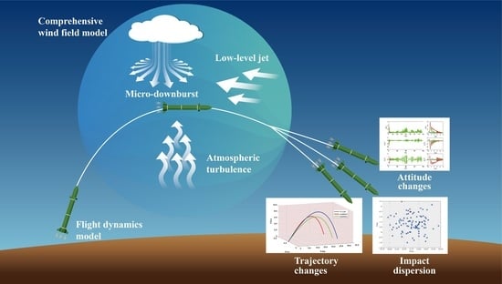
:A complex wind field refers to the typical atmospheric disturbance phenomena existing in nature that have a great influence on the flight of aircrafts. Aimed at the issues involving large volume of data, complex computations and a single model in the current wind field simulation approaches for flight environments, based on the essential principles of fluid mechanics, in this paper, wind field models for two kinds of wind shear such as micro-downburst and low-level jet plus three-dimensional atmospheric turbulence are established. The validity of the models is verified by comparing the simulation results from existing wind field models and the measured data. Based on the principle of vector superposition, three wind field models are combined in the ground coordinate system, and a comprehensive model of complex wind fields is established with spatial location as the input and wind velocity as the output. The model is applied to the simulated flight of a rocket projectile, and the change in the rocket projectile’s flight attitude and flight trajectory under different wind fields is analyzed. The results indicate that the comprehensive model established herein can reasonably and efficiently reflect the influence of various complex wind field environments on the flight process of aircrafts, and that the model is simple, extensible, and convenient to use.
1. Introduction
A complex wind field refers to the typical atmospheric disturbance phenomena in nature, for instance gusts, typhoons, wind shear, turbulence and so on, which are closely related to factors such as weather and terrain. In flying aircrafts, rockets, missiles, and airships, etc., the whole flight process is affected by complex wind fields. For example, the flight stability and safety of aircrafts will reduce, and the firing accuracy of rockets and missiles will become worse. Therefore, establishing a computational model of complex wind fields suitable for flight simulation is of great significance to the design of aircraft and the study of flight control.
At present, there are three types of modeling method for complex wind fields. The first method is the wind field data measurement method. The data obtained from this method are authentic and reliable, but the volume of data is large and the computation cost is high. [1,2], respectively, substituted the exploratory data of 14 Atlantic tropical storms from 1982 to 1989 collected by the Hurricane Research Division (HRD) and the wind vector data from the HY-2 satellite into the wind field data model of the National Center for Environmental Prediction (NCEP) for calculation, analysis and verification. [3] used particle filter and Monte Carlo methods to process the measured data and set up the wind velocity model. [4] reanalyzed the atmospheric circulation data taken from the Black Sea region during the period of 1958 to 2001 and established the distribution of circulation wind field affected by sea temperature. The second method is the numerical method of atmospheric dynamics, which needs to solve the computation-heavy nonlinear differential equations, due to which the methodology is too complicated. [5] used the mesoscale model (MM5) of the National Center for Atmospheric Research of Pennsylvania State University to calculate the distribution of low-level winds located over Antarctica. [6] used the RNG turbulence closure model along with the SIMPLEC pressure correction algorithm to establish the nature of wind field distribution around different buildings. The third method is the engineering simulation method. This method begins with the flow characteristics of airflow in various wind fields and describes the law of airflow movement with simple fluid dynamics equations. This method is simple and intuitive, and can highlight the influence of primary physical parameters. For example, refs. [7,8,9] built the engineering models of micro-downburst using the vortex ring method and wind profile model, respectively. Ref. [10] established a wind distribution model over a large-scale ridge with temperature as the vertical coordinate, and [11,12] developed the atmospheric turbulence models for flight simulation. In the actual flight simulation applications, it is frequently necessary to quickly adjust the parameters according to the changing flight environments to complete the simulation. As a result, it is difficult for both the measured wind field data method and the atmospheric dynamics numerical method to meet such real-time and fast-paced requirements. The engineering simulation method has been widely used because of its simplicity and low computation requirement [13,14,15,16].
It can be seen from the above discussion about the available literature that there are two major deficiencies in the current research on wind field modeling in flight environment. Firstly, the model is relatively simple, because it considers only one form of wind field, and neglects the case that the natural wind appears simultaneously in the form of wind shear, turbulence, and other forms under the influence of terrain and weather. Secondly, owing to the large volume of model data and the complex calculations, special fluid dynamics analysis software is needed. Additionally, it is difficult to meet the requirements of fast simulation or real-time simulation in some practical engineering applications. To address these problems, in this paper, the wind field models of two typical types of wind shear, namely micro-downburst and low-level jet, and atmospheric turbulence are established by the using engineering simulation method. Then, taking the ground coordinate system as the unified reference coordinate system, the three wind field models are combined together to construct a comprehensive wind field model with spatial location coordinates as the input and the wind velocity as the output. Finally, the ballistic simulation of a rocket projectile is used as an example to verify the practicability and efficiency of the comprehensive wind field models.
2. Typical Wind Field Models
2.1. Micro-Downburst
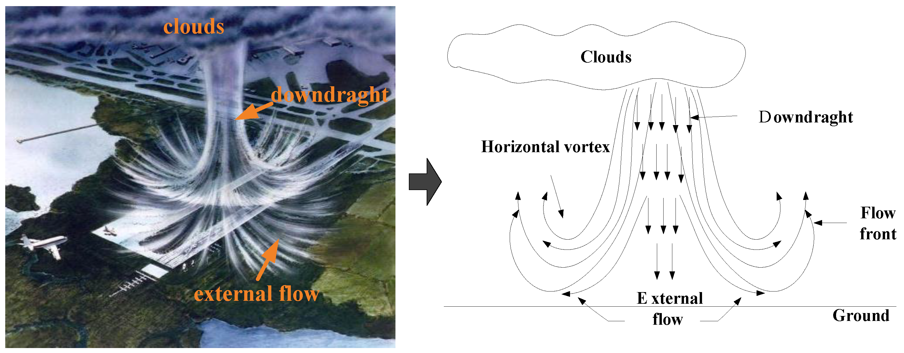
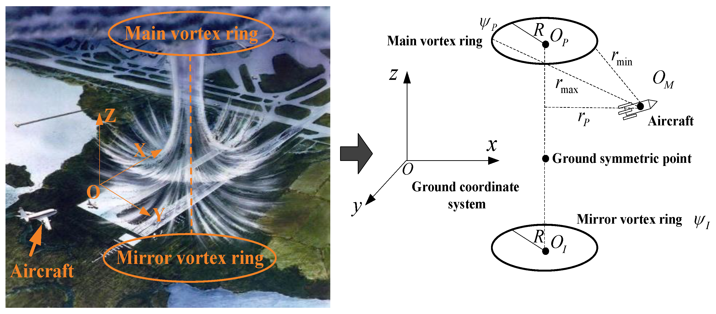
A micro-downburst (abbreviated as MD in this section) is a type of low-level wind shear associated with convective weather [17,18]. Figure 1 shows a schematic diagram of airflow distribution in the MD wind field. It can be noticed that the MD manifests itself as a local vertically downward airflow in the strong convective cloud cluster. After the airflow sinks and touches the ground, it diverges in all directions and curls up to form an area of vortex ring above the ground. In view of such flow characteristics, a bunch of ground-symmetric vortex rings were constructed in the vertical direction of the horizontal plane to simulate the vertical airflow generation [19]. The coordinate system of the model is illustrated in Figure 2.
Considering the ground coordinate system as the datum and a point above the plane as the center, a closed vortex ring of radius is set, named the main vortex ring, and its curve equation is:
The circulation line equation of the main vortex is:
where denotes the intensity of the vortex ring, determined by vertical velocity of the vortex ring center and the vortex ring radius :
and are the maximum and the minimum distances of the main vortex ring from an arbitrary point in the ground coordinate system, and is the elliptic integral function, where:
Based on the theories of higher functions [7], when , is approximated as:
Based on Equation (2), the induced radial and axial velocities of the main vortex ring can be calculated by partial derivatives:
where is distance of the point from the axis of vortex ring (). By decomposing the induced velocities calculated by Equation (6) along the and axes of the ground system, the velocity components can be written as:
In the actual circumstances, the vertical velocity component on the ground should be zero after the vertical airflow of the vortex ring center reaches the ground. For that reason, by setting the method of mirror vortex ring for the symmetry of main vortex ring about the plane , the vertical induced velocities on the ground are reversed with equal value and thus cancel each other out. The signs of the streamline equations for the two vortex rings are opposite . Given the mirrored vortex ring center , its connection line with the main vortex ring center is vertical to the ground. According to the streamline equation of the mirrored vortex ring, analogous to the derivation of the induced velocity of the main vortex ring, the induced velocities at the spatial points of the mirrored vortex ring can be calculated. Velocity superposition is performed by combining Equations (6) and (7), and the resultant velocity at point can be obtained as:
Then, the streamline equation of point is:
where and denote the maximum and the minimum distances of the mirrored vortex ring from the spatial point , and similarly .
The simulation results of the model are shown in Figure 3. It can be noted that the simulated wind field distribution of the vortex ring model is consistent with the measured data.
2.2. Low-Level Jet
Low-level jet (abbreviated as LLJ in this section) refers to the wind velocity zone in the lower troposphere, which is significantly affected by the mesoscale weather system. It is a surface inversion phenomenon occurring in the stable surface boundary layer [23]. According to the principle of the plane wall jet, when a plane free jet with a large width flows through a narrow slit, the velocity distribution of the jet near the wall is similar to that of the LLJ [24]. For that reason, the plane wall jet is employed to simulate the wind velocity distribution of the LLJ wind field, as shown in Figure 4.
According to the principles of fluid dynamics, the relationship between the horizontal velocity component of a free jet and its maximum jet velocity is:
where denotes a scale factor and refers to hyperbolic tangent function. To simplify the model, the basic flow characteristics of LLJ are retained, while the wind velocity is evenly distributed in the horizontal direction , that is,
where denotes the height of maximum velocity of the free jet with symmetrical distribution, is employed to describe the relationship between and the width of the jet in the vertical direction; and the width of jet denoting the velocity range determined by 7% of the maximum velocity. The expression is
By superimposing the velocity distribution of the free jet onto the exponential model of the mean wind in the boundary layer, the vertical velocity profile of LLJ on the surface boundary layer can be obtained:
In the formula above, is the wind velocity corresponding to the height of , where the distribution index can be calculated in keeping with the relevant meteorological data [25]:
where denotes terrain roughness; analogous to Equation (13), the deviation of wind direction between height and height is derived as:
where , and denote reference height, height of maximum deviation of wind direction in the jet stream layer and height of top of the jet stream layer, respectively; , and are the angles included between the wind direction and the geostrophic wind at the three corresponding heights, respectively; and are wind velocities at heights and , respectively.
Thus, the wind velocity components in the ground coordinate system are calculated as:
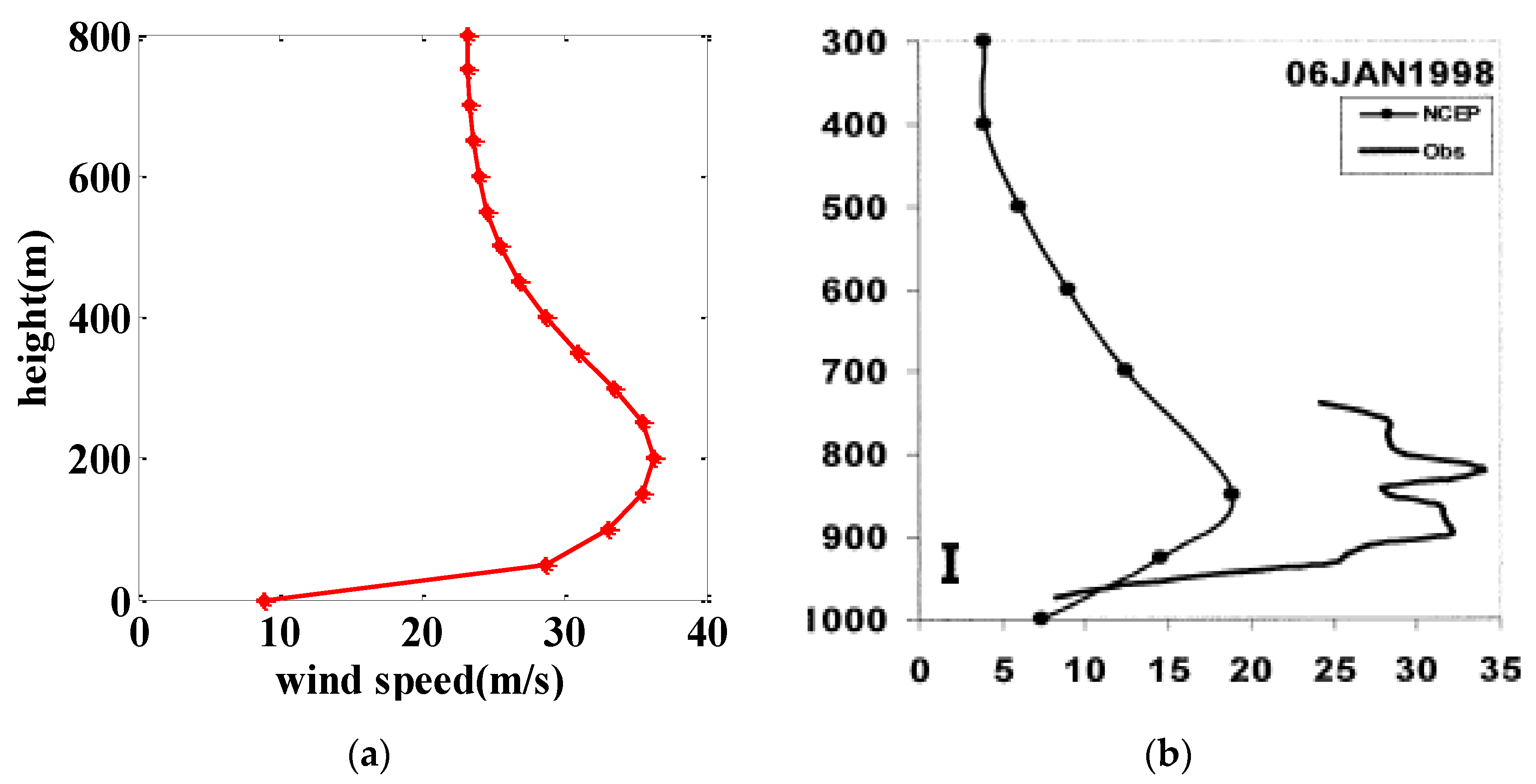
The model parameters [26] are configured as shown in Table 2 and the simulation results are shown in Figure 5.
It can be seen from Figure 5a,b that the wall jet model can accurately simulate the wind velocity distribution of the actual LLJ wind field.
2.3. Atmospheric Turbulence
Atmospheric turbulence is the irregular and uneven random eddy motion of the Earth’s atmosphere. The Dryden model is a classical form of atmospheric turbulence, wherein the longitudinal and transverse correlation functions [28] are expressed as:
The spatial correlation function [29] of one-dimensional turbulence is:
For two (or three)-dimensional turbulence, the spatial correlation function is:
where denotes the location difference between the two spatial points, , , are the components of in the ground coordinate system, is the turbulence intensity parameter, is the turbulence scale parameter, and the subscripts , , denote the components of turbulent velocity in the ground coordinate system.
For a one-dimensional turbulent sequence, the recursion equation is:
where denotes the turbulent velocity along the one-dimensional direction, is the one-dimensional white noise sequence, is the simulation step size, and are the recursion parameters to be solved. According to the correlation function definitions of the Dryden model,
Combining Equations (18) and (21), where , it is obtained that
Thus, the one-dimensional atmospheric turbulent velocity can be calculated. Similarly to Equation (20), the recursion equation of two-dimensional turbulence can be written as:
The correlation function values are
The equation obtained by expanding Equation (24) is
Substitute calculated by Equation (19) into Equation (25), where , so that the parameters can be obtained. Thus, the two-dimensional atmospheric turbulent velocity can be calculated according to the recursive Equation (23).
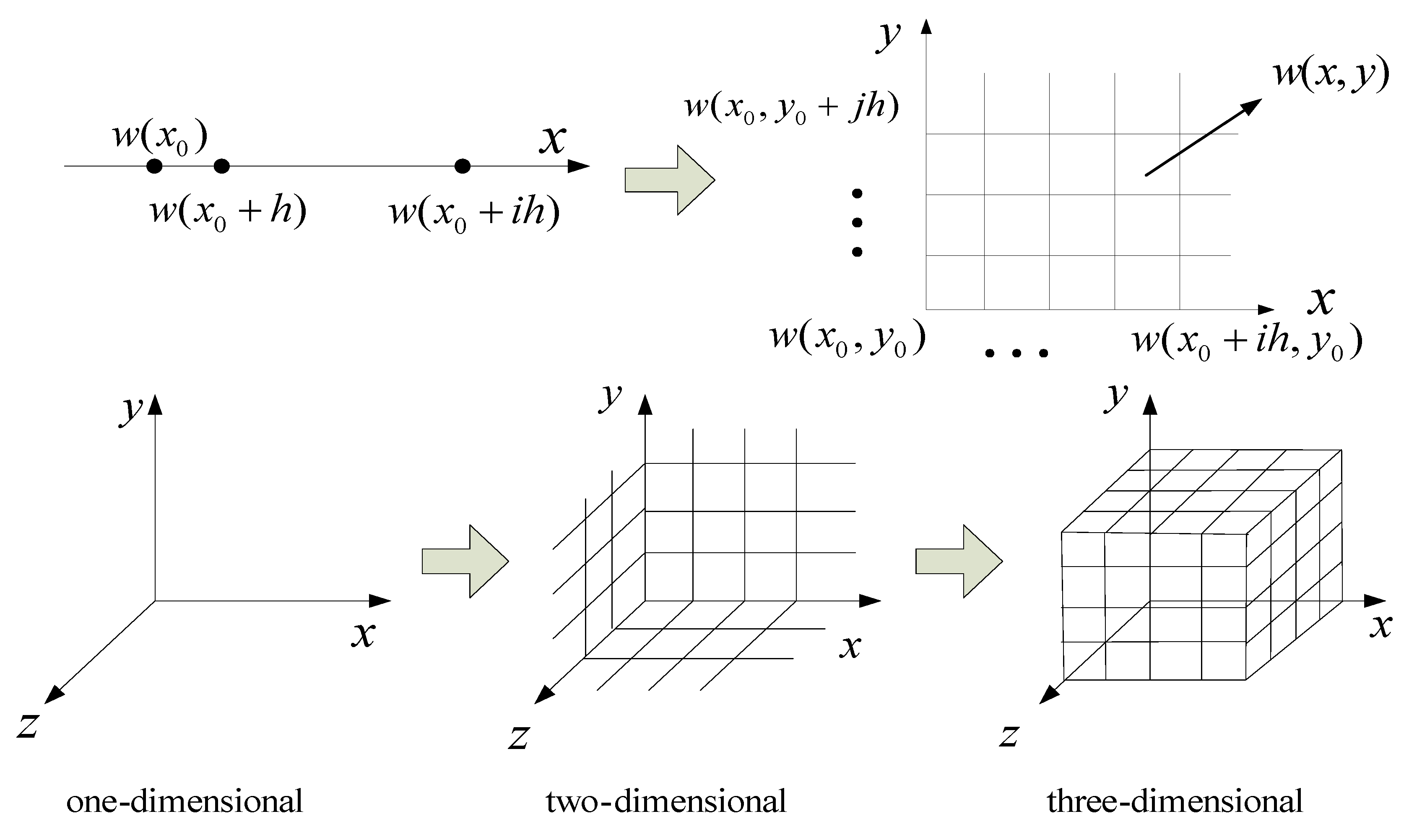
For the three-dimensional space turbulence, the construction idea is as follows: taking one-dimensional turbulence as the boundary value to figure out the two-dimensional plane turbulence sequence, and subsequently taking the two-dimensional plane turbulence sequence as the boundary value to figure out the three-dimensional space turbulence, as shown in Figure 6.
Analogous to Equations (20) and (23), the three-dimensional turbulence recursion equation is formulated as
The correlation function of the three-dimensional space turbulence can be expressed as
Substituting Equation (19) into Equation (27), where , the following equations are obtained
By solving Equation (28), the recursive parameters and can be obtained, and then the velocity recursion equation of three-dimensional space turbulence is obtained. By using the method above, and can also be obtained. AT refers to the atmospheric turbulence herein.
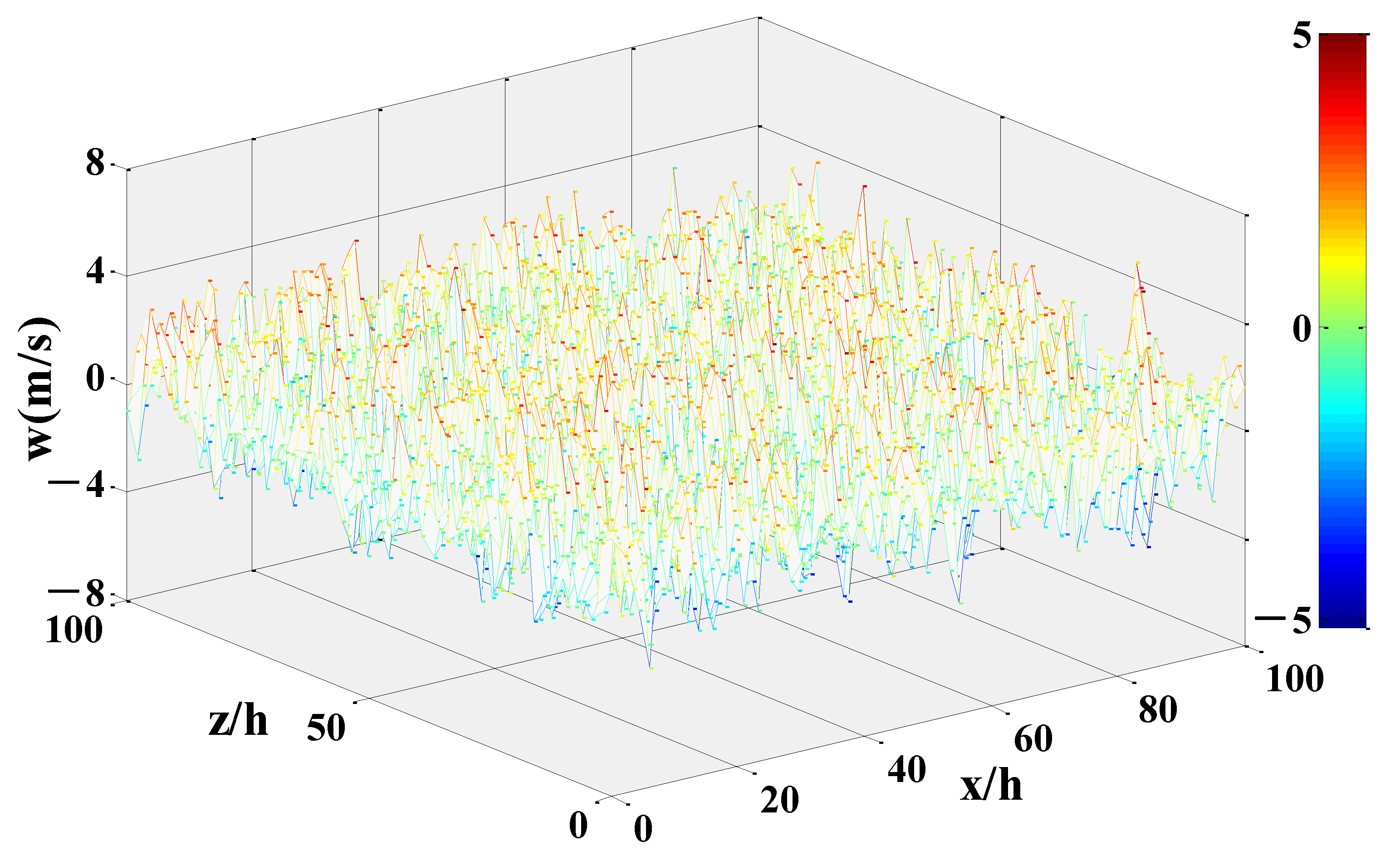
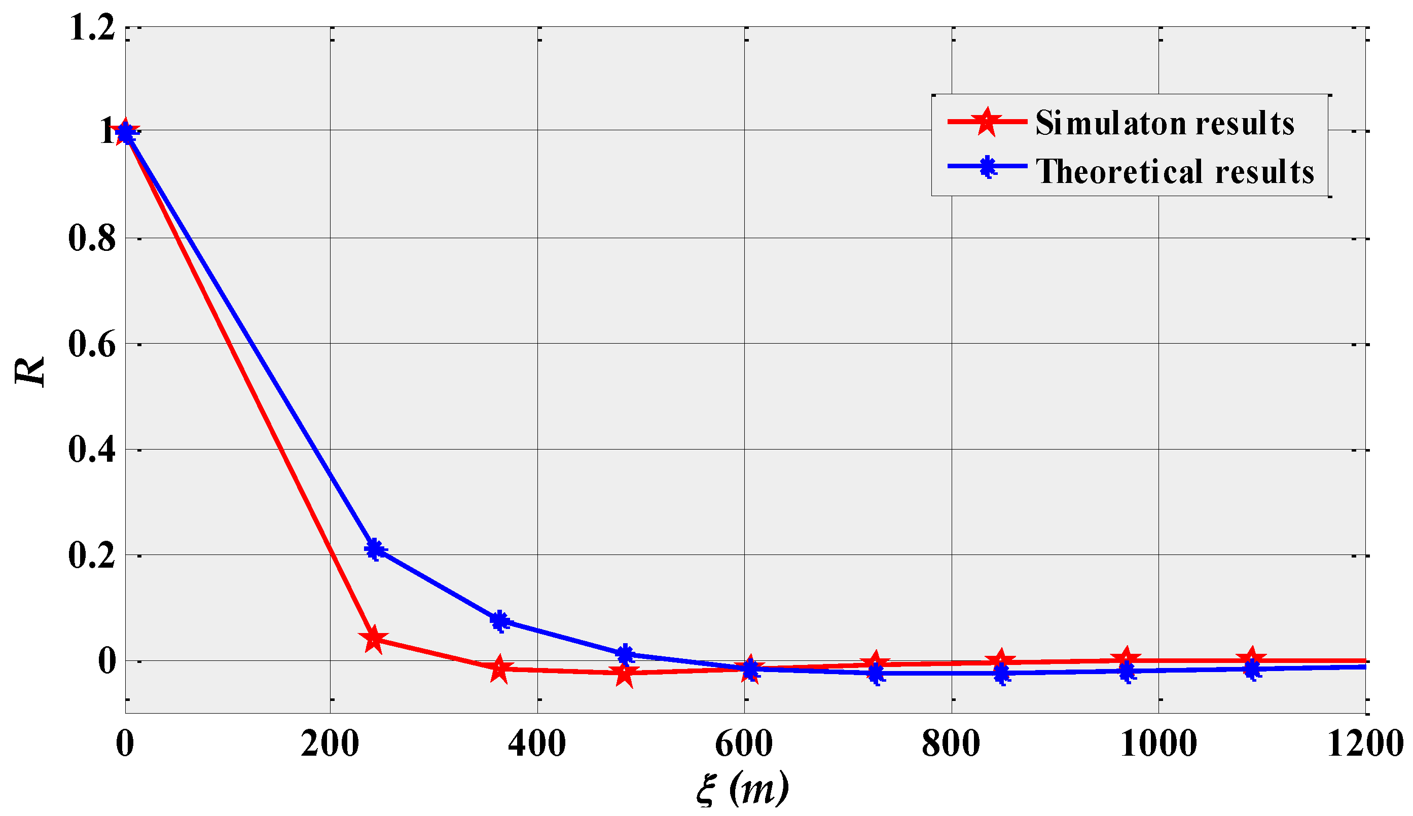
According to the parameters in Table 3, the three-dimensional atmospheric turbulence was simulated in space. The simulation results are shown in Figure 7 and Figure 8. From Figure 8, the random variation of the atmospheric turbulent wind velocity in space is observed. As presented in Figure 8, the theoretical value is calculated according to correlation function (Equation (19)) of the Dryden model. It can be seen that the variation trend in the correlation value of turbulent velocity simulated by simulation is actually the same as that obtained from the Dryden model, which proves the rationality and effectiveness of the established model.
3. Comprehensive Wind Field Model
Since wind velocity is a vector including magnitude and direction, it meets the principle of vector superposition. For any spatial point , assuming that wind field induces the wind velocity vector at point and wind field induces the wind velocity vector at point , the total wind velocity vector at point induced by the wind fields and can be obtained by the following equation:
Based on Equation (30), in this section, a superposition method is adopted to synthesize the established typical wind field models. The input and output parameters of the three typical wind field models are listed in Table 4.
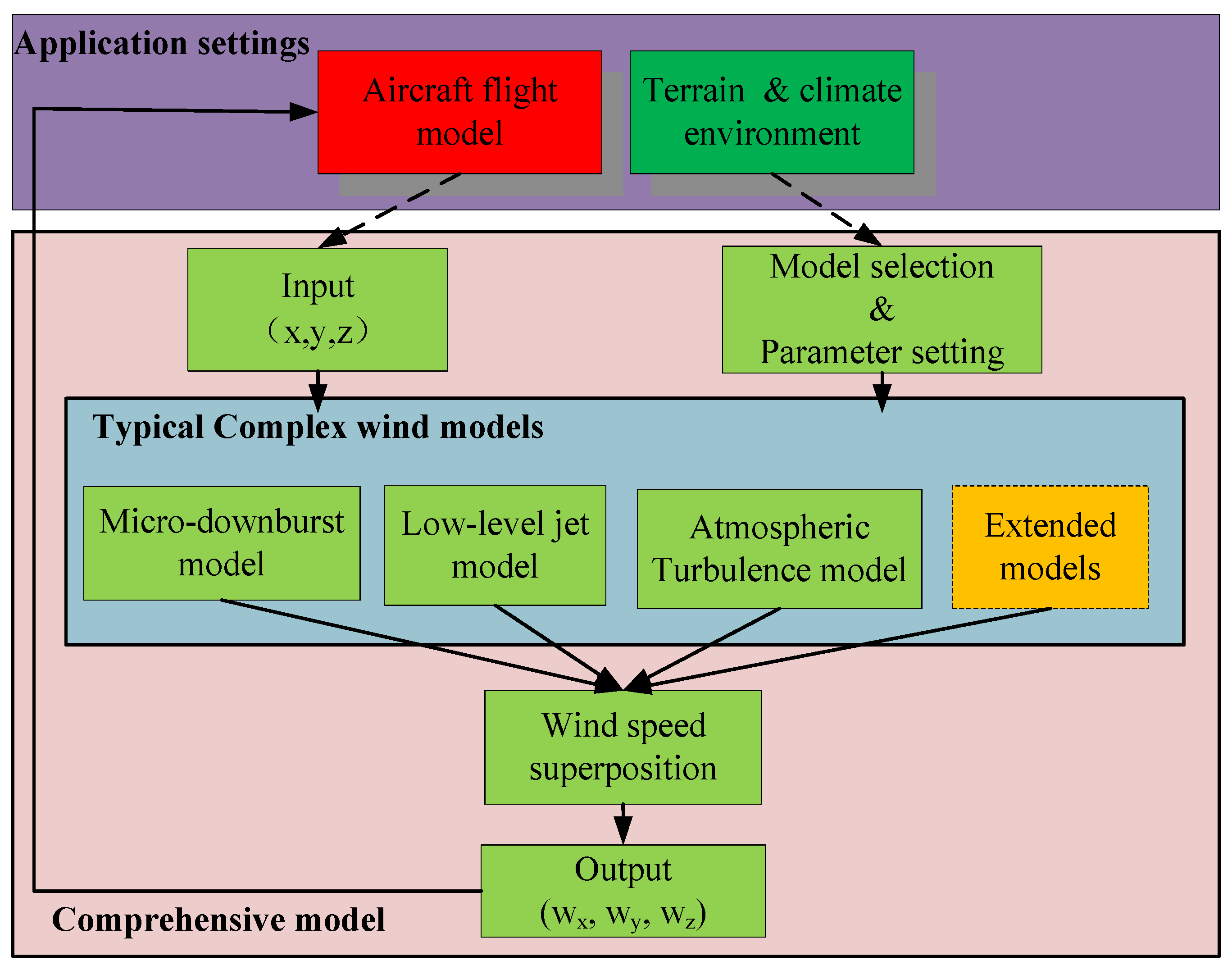
It can be seen that the inputs of the three models are the spatial positions, and the outputs are the wind velocity components. Therefore, the inputs and outputs are combined, and the ground coordinate system is used as the frame of reference to establish a comprehensive model. The application structure of this model is shown in Figure 9.
As can be seen from Figure 9, the calculation process of the comprehensive wind field model consists of four key steps:
- Input spatial location parameters;
- Select the wind field models according to simulation requirements;
- Calculate the total wind velocity value;
- Substitute the wind velocity into the flight simulation.
To ensure the scalability of the model, an expansion module (yellow box in the chart) is set up to add other wind field models such as gust and mountain flow.
4. Model Application
4.1. Flight Simulations under Different Wind Field Conditions
In order to verify the calculation effect on the whole model, a rocket projectile is taken as an example and the six degrees-of-freedom rigid body trajectory equation of the rocket projectile is considered as the flight simulation model. The basic parameters [31] of the rocket projectile are listed in Table 5.
For the flight state of a rocket projectile, the main concern is its trajectory and flight attitude. The flight trajectory can be directly analyzed by calculating the three-dimensional trajectory curve of the rocket projectile, while the flight attitude needs to be reflected by the flight attack angle.
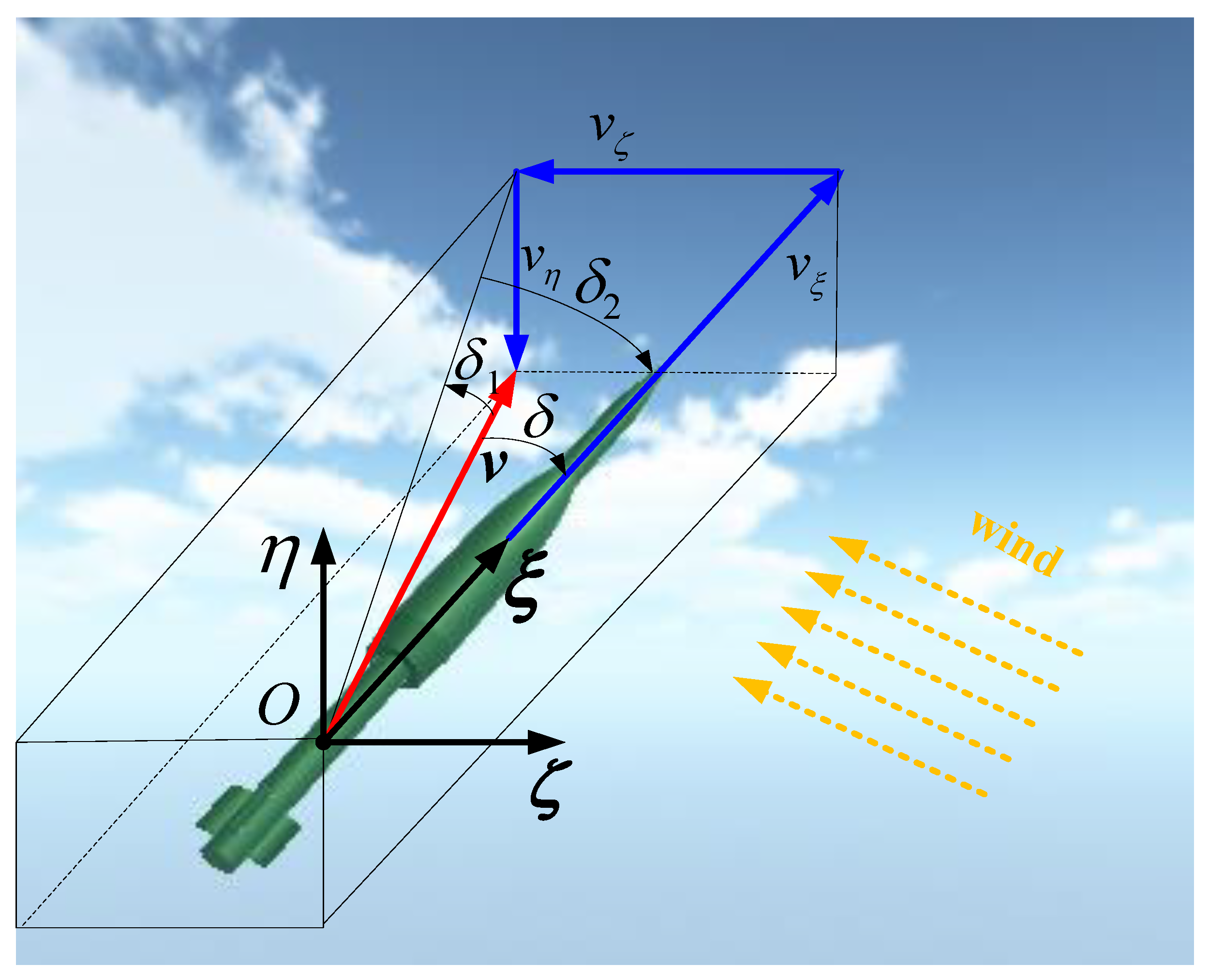
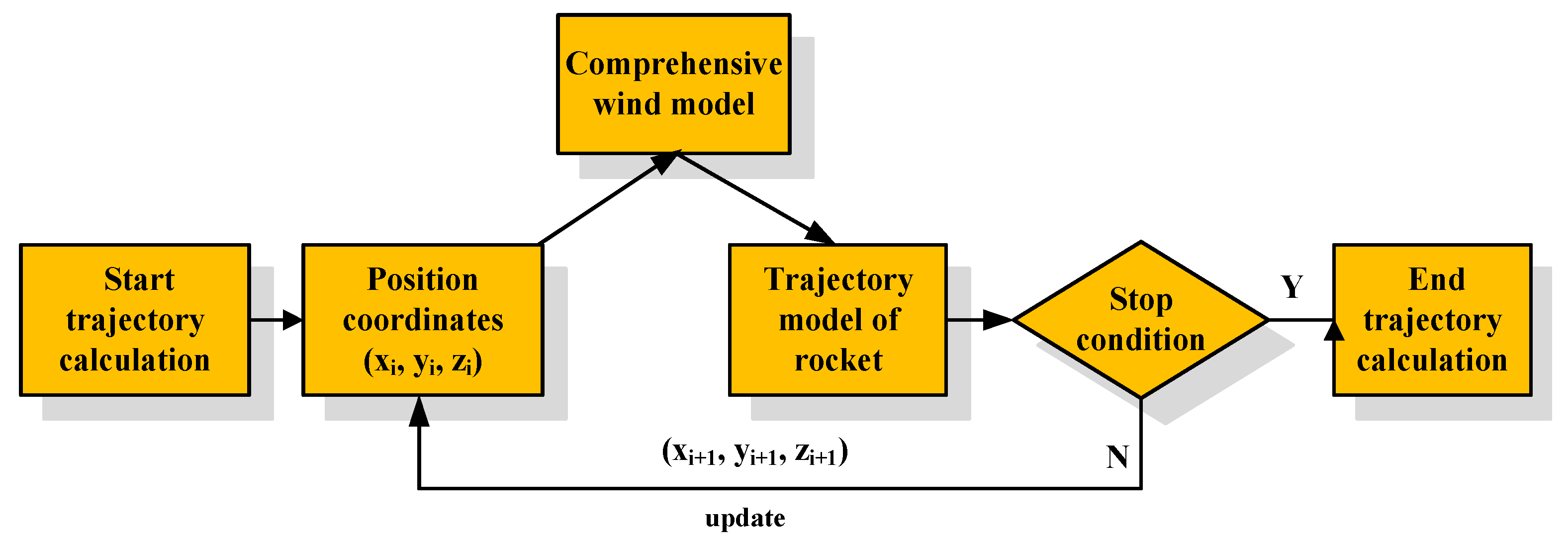
Figure 10 shows the conceptual schematic diagram of the attack angle of rocket, where the coordinate system is taken as the reference coordinate system, is the center of rocket mass, the axis coincides with the axis of the rocket, the axis points vertically upward, and the axis is determined according to the right hand rule. The red vector denotes the velocity of the rocket’s centroid, the blue vector represents the three components , and of in the coordinate system , represents the angle included between the rocket axis and the velocity , and is called the total attack angle, is called the pitch attack angle, and is called the direction attack angle. The attack angles , and of the rocket describe the positional relationship between the projectile axis and the velocity direction during the flight of the rocket. Through the curve of the attack angle, the attitude changes and the stability of the rocket during the flight can be seen. The specific flight simulation calculation steps are shown in Figure 11.
While using the integral method to solve the trajectory, the coordinates of the rocket’s position within each calculation step are substituted into the wind field model to obtain the wind velocity, which is then substituted into the trajectory equations to calculate the next trajectory parameters. These trajectory parameters include the position coordinates in addition to attack angles of the rocket projectile. The detailed solution of the trajectory equations can be found in the literature [31] (pp. 141–143). Table 6 lists two wind field conditions employed for flight simulation of a rocket projectile. The flight processes under the two wind field conditions are simulated, and are compared with the flight state of the rocket projectile under windless condition.
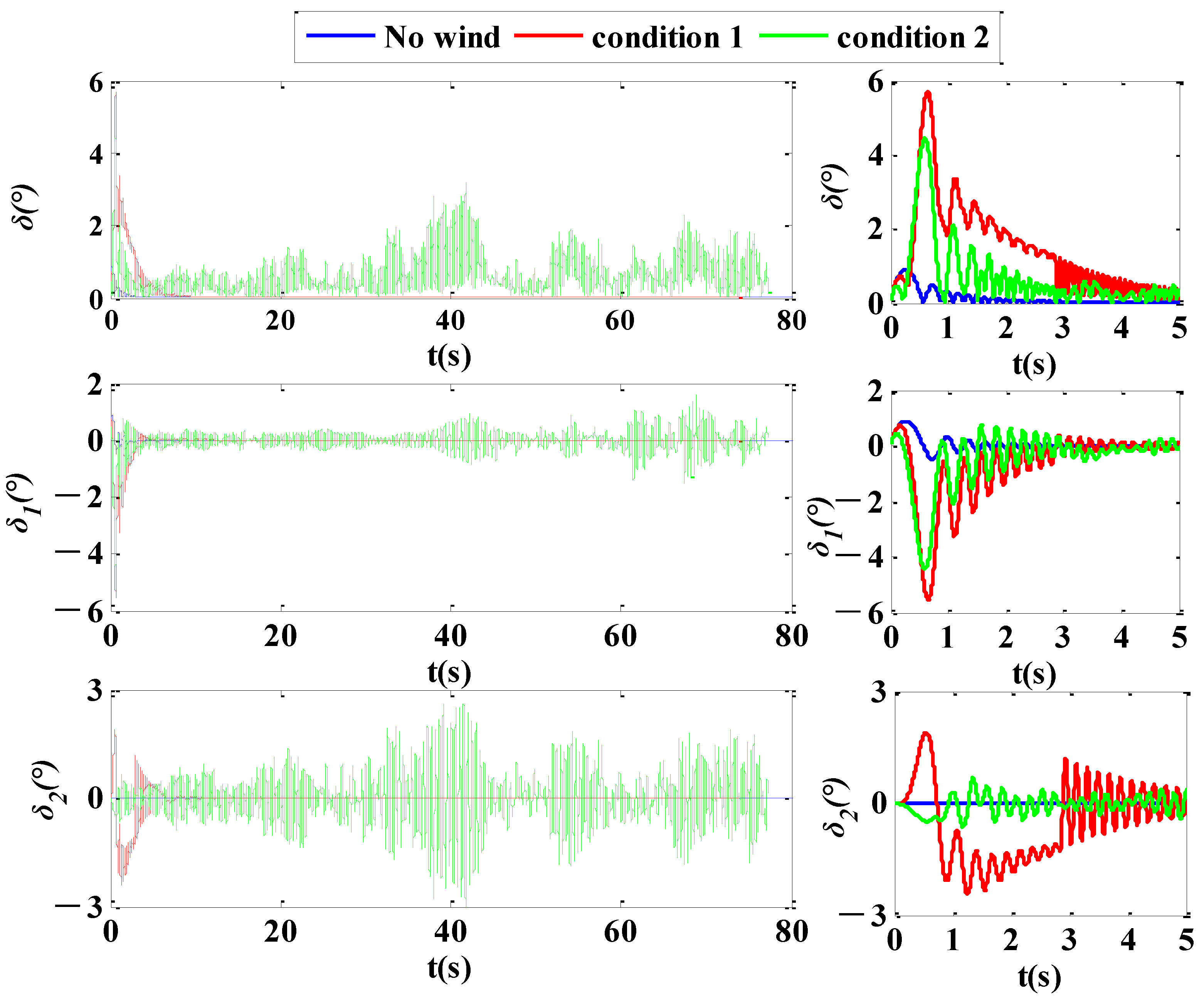
Figure 12 shows the change curves of the attack angles of the rocket projectile with flight time under the influence of the two wind fields listed in Table 6. The one on the left-hand side of the figure is the attack angle of the whole trajectory, while the small one on the right-hand side is the local attack angle of the first 5 s of the trajectory. It can be noticed that in a windless environment, the amplitude of attack angle of rocket projectile persistently decreases with the increase in the flight time and converges to nearly 0 degrees, indicating that the flight attitude of the rocket projectile gradually tends to become stable. Under the influence of the low-level jet in condition 1, the rocket projectile has a low velocity and weak anti-interference capability in the initial stages of launch. So, the amplitude of attack angle increases suddenly under the action of transient but strong airflow. As the rocket projectile continues to fly, the attack angle converges in a similar way as it would in a windless condition. Under the influence of the MD in condition 2, the attack angle of the rocket projectile also increases suddenly, similar to that observed in condition 1. However, due to the influence of the atmospheric turbulence at the same time, the amplitude of attack angle cannot converge further, fluctuates continuously, and the flight attitude is not stable anymore.
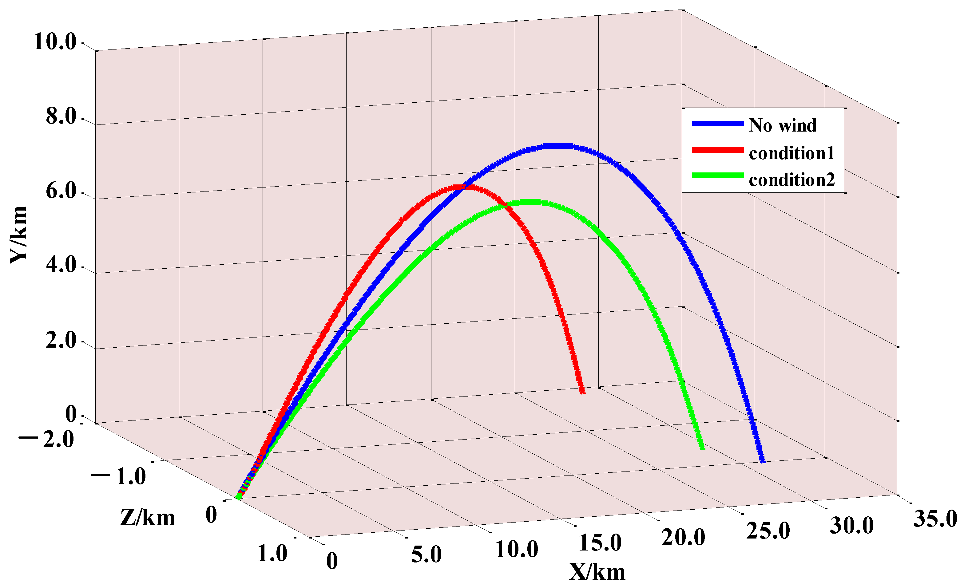
Figure 13 shows the three-dimensional curve of flight trajectory of rocket projectile under wind field condition 1, wind field condition 2 and the windless environment. As can be seen from Figure 13, under the influence of conditions 1 and 2, the maximum trajectory height of the rocket projectile decreases, the range decreases, and the whole flight trajectory deviates significantly. In particular, the lateral deviation of the landing point under the influence of condition 1 increases much more than that under condition 2, which reflects the difference in the influence of the two wind conditions.
Figure 14 shows the dispersion of the rocket projectile under the influence of condition 2 using the Monte-Carlo method.
According to the flight simulation results shown in Figure 12, Figure 13 and Figure 14, it can be concluded that the comprehensive model of complex wind field established herein, can reflect the law of influence of different wind fields on the aircraft when applied in flight simulation, which reflects the practicability and rationality of the model.
4.2. Analysis on Influence of Different Model Parameters on Flight Process
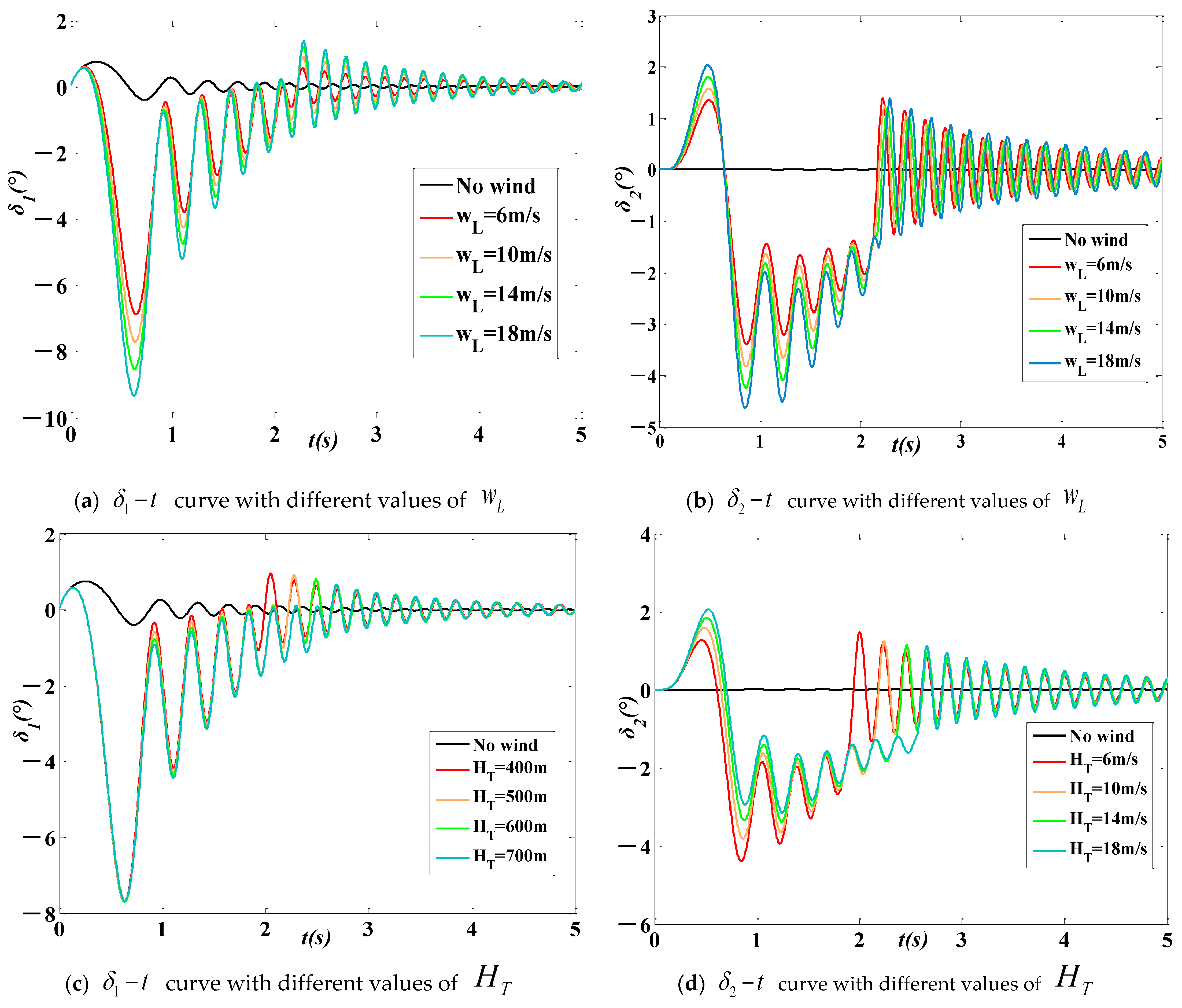
For a certain kind of typical wind field, it is necessary to study the effect of different model parameters on the flight process of aircrafts. Taking the low-level jet wind field(condition 1 in Section 4.1) as an example, the simulations are made with different values of (strength parameter) and (scale parameter). The main ballistic parameters of simulations are listed in Table 7 and Table 8. The attack angle curves (within the first 5 s of the flight trajectory) of and are shown in Figure 15.
From Table 7 and Table 8, it can be seen that the ballistic characteristics changed under the influence of low-level jet. The changes are specifically manifested in the reduction in flight time and terminal velocity, the decrease in down range and the increase in cross range (the order of magnitude from 10 to 103). The simulation results also show that the influence degree of low-level jet on the flight process is positively correlated to the strength parameter and the scale parameter .
From the attack angle curves in Figure 15, the attitude changes of the rocket projectile under different wind field model parameters can be directly observed. It is shown that the low-level jet causes a sudden change and a convergence process of the attack angle of the attack angle , which result in the large change in the cross range (in Table 7 and Table 8) of the rocket.
4.3. Discussions of Use Conditions of the Comprehensive Model
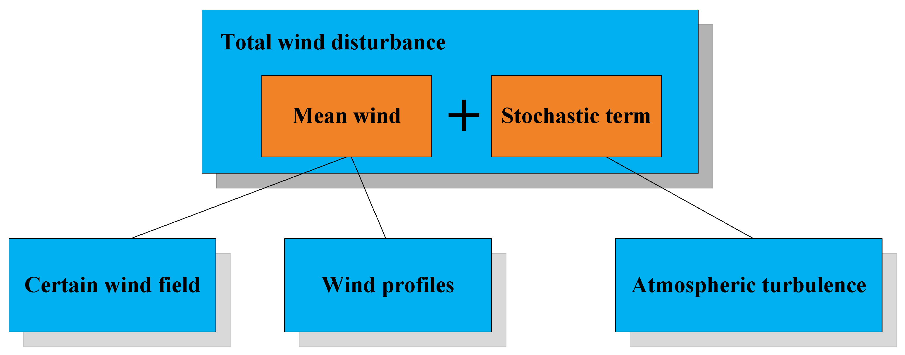
In fact, the real wind field in nature changes not only in space but also in time, which can significantly influence the accuracy of flight simulation. It is necessary to give some conditions of use for the established comprehensive model. According to the atmospheric dynamics [25], the wind field disturbance can be expressed as:
Equation (31) indicates that the total disturbance is composed of the mean wind and the stochastic term . In the conditions of small time and spatial scales, can be described as a certain wind field, such as micro-downburst, and the wind profile, , can be described as the atmospheric turbulence. The diagram is shown in Figure 16.
Based on Figure 16, the conditions of use for the established comprehensive model are given as:
- When the flight simulation is in a small time scale (in condition 1 of Section 4.1, the rocket went through the low-level jet area within 2 s) or in a small spatial scale (the low-level jet area has a height of 800 m and the rocket has a flight altitude of 10 km), the established comprehensive model can be used to obtain some reasonable results.
- When the flight simulation is in a large time scale (or in a large spatial scale), such as the total flight process of a long-range missile, an airplane or an airship, the comprehensive model might cause significant errors.
5. Conclusions
Built on the basic principles of fluid mechanics, the engineering wind velocity calculation models of three typical wind fields, namely micro-downburst, low-level jet and atmospheric turbulence, are herein established. By combining the three models in the ground coordinate system and unifying the input and output parameters, a comprehensive model of complex wind field is established. The wind field model simulation and application simulation indicate that the comprehensive model can reasonably and effectively describe the flow characteristics of the relevant wind field, and has the characteristics of simple calculation and model scalability. Additionally, as shown in Section 4.2, the comprehensive model can be used not only to analyze the influence of different wind fields on the flight process, but also to study the influence of different model parameters on the flight simulations.
As an important factor of the simulation accuracy of the wind field model, the wind field data collection methods in different time and space scales of the simulated flights are the main points of our further research. Meanwhile, developing a reasonable wind field model for large time and space scales with the least amount of collection data is also an extension of the work in this paper.
Author Contributions
Conceptualization, J.C.; methodology, J.C.; software, J.C., Z.Y.; validation, J.C.; formal analysis, J.C. and J.F..; investigation, J.C. and J.F.; resources, J.C. and Z.Y.; writing—original draft preparation, J.C.; writing—review and editing, J.C.; supervision, L.W. and J.F.; project administration, L.W.; funding acquisition, L.W. All authors have read and agreed to the published version of the manuscript.
Funding
This research was funded by the National Science Foundation of China (No. 61603191).
Data Availability Statement
Not applicable.
Conflicts of Interest
The authors declare no conflict of interest.
References
- Tuleya, R.E.; Lord, S.J. The Impact of Dropwindsonde Data on GFDL Hurricane Model Forecasts Using Global Analyses. Weather Forecast. 2010, 12, 307–323. [Google Scholar] [CrossRef] [Green Version]
- Bo, M.; Lin, M.; Peng, H. WindSim Computational Flow Dynamics Model Testing Using Databases from Two Wind Measurement Stations. Electronics 2011, 15, 63–70. [Google Scholar]
- Klisić, Đ.; Zlatanović, M.; Radovanović, I. Validation of wind vectors retrieved by the HY-2 microwave scatterometer using NCEP model data. Eng. Sci. 2014, 2, 39–61. [Google Scholar]
- Efimov, V.V.; Anisimov, A.E. WindSim Climatic parameters of wind-field variability in the Black Sea region: Numerical reanalysis of regional atmospheric circulation. Izv. Atmos. Ocean. Phys. 2011, 47, 350–361. [Google Scholar] [CrossRef]
- Parish, T.R.; Cassano, J.J. Diagnosis of the Katabatic Wind Influence on the Wintertime Antarctic Surface Wind Field from Numerical Simulations. Mon. Weather Rev. 2003, 6, 1128–1139. [Google Scholar] [CrossRef]
- Zhang, A.; Gao, C.; Ling, Z. Numerical simulation of the wind field around different building arrangements. J. Wind Eng. Ind. Aerodyn. 2005, 12, 891–904. [Google Scholar] [CrossRef]
- Ivan, M. Ring-vortex downburst model for flight simulations. J. Aircr. 2012, 3, 232–236. [Google Scholar] [CrossRef]
- Zhang, W.F.; Xie, D.; Liu, Y.C.; Jing, J.I. Simulation of downburst wind field with spatial correlation. J. Vib. Shock. 2013, 32, 12–16. [Google Scholar]
- Jesson, M.; Sterling, M. A simple vortex model of a thunderstorm downburst—A parametric evaluation. J. Wind Eng. Ind. Aerodyn. 2018, 174, 1–9. [Google Scholar] [CrossRef]
- Eliassen, A.; Thorsteinsson, S. Numerical studies of stratified air flow over a mountain ridge on the rotating earth. Tellus A 2010, 2, 172–186. [Google Scholar]
- Ji, H.; Chen, R.; Li, P. Distributed Atmospheric Turbulence Model for Helicopter Flight Simulation and Handling-Quality Analysis. J. Aircr. 2017, 54, 190–198. [Google Scholar] [CrossRef]
- Jansen, C.J. Non-Gaussian Atmospheric Turbulence Model for Flight Simulator Research. J. Aircr. 2012, 19, 374–379. [Google Scholar] [CrossRef]
- Towers, P.; Jones, B.L. Real-time wind field reconstruction from LiDAR measurements using a dynamic wind model and state estimation. Wind Energy 2016, 19, 133–150. [Google Scholar] [CrossRef] [Green Version]
- Fluck, M.; Crawford, C. An engineering model for 3D turbulent wind inflow based on a limited set of random variables. Wind Energy Sci. Discuss. 2017, 1, 1–20. [Google Scholar]
- Lupi, A.; Hans, J.; Niemann, B. Aerodynamic damping model in vortex-induced vibrations for wind engineering applications. J. Wind Eng. Ind. Aerodyn. 2018, 9, 14–24. [Google Scholar] [CrossRef]
- Albini, F.A. A Phenomenological Model for Wind Speed and Shear Stress Profiles in Vegetation Cover Layers. J. Appl. Meteorol. Clim. 2010, 11, 1325–1335. [Google Scholar] [CrossRef] [Green Version]
- Lianlei, L.; Xilin, L.; Gang, W. Modelling of Microburst Based on the Slanted Vortex-Ring Model. Chin. J. Electron. 2018, 27, 318–323. [Google Scholar]
- Dogan, A.; Kabamba, P.T. Escaping Microburst with Turbulence: Altitude, Dive, and Pitch Guidance Strategies. J. Aircr. 2015, 37, 417–426. [Google Scholar] [CrossRef]
- Lundgren, T.S.; Yao, J.; Mansour, N.N. Microburst modelling and scaling. J. Fluid Mech. 2006, 239, 461–488. [Google Scholar] [CrossRef]
- Xhelaj, A.; Burlando, M.; Solari, G. A general-purpose analytical model for reconstructing the thunderstorm outflows of travelling downbursts immersed in ABL flows. J. Wind Eng. Ind. Aerodyn. 2020, 207, 1–7. [Google Scholar] [CrossRef]
- Proctor, F. Model comparison of July 7, 1990 microburst. In Proceedings of the Third Combined Manufacturer’s and Technology Airbone Windshear Review Meeting, Hampton, VA, USA, 1 January 1991. [Google Scholar]
- Wanke, C.R.; Hansman, J.R. A data fusion algorithm for multi-sensor microburst hazard assessment. In Proceedings of the AIAA Atmospheric Flight Mechanics Conference, Hilton Head Island, SC, USA, 10–12 August 1992. [Google Scholar]
- Wang, H.; Fu, R. Influence of Cross-Andes Flow on the South American Low-Level Jet. J. Clim. 2002, 17, 1247–1262. [Google Scholar] [CrossRef]
- Wang, C.; Wang, Z.S.; Li, Z.L. Comparison and parametric analysis of wind profile characteristics of impinging jet and wall jet. Eng. Mech. 2015, 32, 86–93. [Google Scholar]
- Xiao, Y.L. Flight Principle in Atmospheric Turbulence, 1st ed.; National Defense Industry Press: Beijing, China, 1993; pp. 27–47. [Google Scholar]
- Chen, J.; Wang, L.; Li, Z. Influence of two typical kinds of low-level wind shear on ballistic performance of rockets. J. Beijing Univ. Aeronaut. Astronaut. 2018, 44, 1008–1017. [Google Scholar]
- Marengo, J.A.; Soares, W.R.; Saulo, C.; Nicolini, M. Climatology of the Low-Level Jet East of the Andes as Derived from the NCEP–NCAR Reanalyses: Characteristics and Temporal Variability. J. Clim. 2004, 17, 12–19. [Google Scholar] [CrossRef] [Green Version]
- Beal, T.R. Digital Simulation of Atmospheric Turbulence for Dryden and von Karman Models. J. Guid. Control. Dynam. 1993, 16, 132–138. [Google Scholar] [CrossRef]
- Jing, G.; Guanxin, H.; Zaoqing, L. Theory and method of numerical simulation for 3D atmospheric turbulence field based on Von Karman model. J. Beijing Univ. Aeronaut. Astronaut. 2012, 38, 736–740. [Google Scholar]
- Halsig, S.; Artz, T.; Iddink, A.; Nothnagel, A. Using an atmospheric turbulence model for the stochastic model of geodetic VLBI data analysis. Earth Planets Space 2016, 68, 106. [Google Scholar] [CrossRef] [Green Version]
- Han, Z.P. Exterior Ballistics of Shells and Rockets, 2nd ed.; Beijing University of Technology Press: Beijing, China, 2008; pp. 141–143. [Google Scholar]
Figure 1.
Airflow distribution of micro-downburst.

Figure 2.
Coordinate system of micro-downburst model.

Figure 3.
Comparisons between simulation results and measured data of micro-downburst. (a) Simulation wind vector diagram of horizontal section. (b) Flow pattern of 7 July 1990 Orlando downburst from NTRS-NASA Technical Reports Server [21]. (c) Simulation wind vector diagram of vertical section. (d) Flow pattern of 1988 microburst event of DEN from NTRS-NASA Technical Reports Server [22].

Figure 4.
Diagram of the plane wall jet.

Figure 5.
Comparisons between simulation results and measured data of low-level jet. (a) Wind profiles () of low-level jet by simulation. (b) Wind profiles derived from the NCEP-NCAR reanalyzes and from the PACS-SONET upper-air observations [27] (© American Meteorological Society. Used with permission).

Figure 6.
Construction process of three-dimensional atmospheric turbulence.

Figure 7.
Atmospheric turbulent wind velocity in space (H = 600 m).

Figure 8.
Comparisons of correlation values between simulation results and theoretical calculation.

Figure 9.
Application structure of the comprehensive wind field model.

Figure 10.
Attack angle diagram of the rocket projectile.

Figure 11.
Flight simulation process.

Figure 12.
Attack angle curves of the rocket projectile.

Figure 13.
Trajectories of the rocket projectile under different wind field conditions.

Figure 14.
Impact dispersion of the rocket projectile under the influence of condition 2 (simulation time = 100).
Figure 14.
Impact dispersion of the rocket projectile under the influence of condition 2 (simulation time = 100).

Figure 15.
Attack angle curves with different wind field model parameters.

Figure 16.
Composition of the wind disturbance in small time and spatial scales.


Table 1.
Parameters of micro-downburst model.
| Parameter | Value |
|---|---|
| (1000 m, 0, 800 m) | |
| 1100 m | |
| −10 m/s |
Table 2.
Parameters of low-level jet model.
| 2.5 m | 3.5 m | 5 ms−1 | 180 m | 10 ms−1 | 800 m | 0° | 30° | 60° | 0.8 | 0.3 |
Table 3.
Parameters of atmospheric turbulence model [30].
Table 3.
Parameters of atmospheric turbulence model [30].
| Parameter | Value |
|---|---|
| 150 m | |
| 1.5 ms−1 | |
| 50 m |
Table 4.
Input and output parameters of the three typical wind field models established.
| Wind Field | Input | Output |
|---|---|---|
| Micro-downburst | , , | |
| Low-level jet | , | |
| Atmospheric turbulence | , , |
Table 5.
Basic parameters of the rocket projectile.
| Parameter | Value |
|---|---|
| Diameter of rocket | 0.122 m |
| Length of rocket | 2.9 m |
| Specific impulse | 250 s |
| Working time of the engine | 3 s |
| Initial velocity | 40 ms−1 |
| Firing angle | 50 deg |
| Firing direction | 0 deg |
Table 6.
Simulation conditions of complex wind field.
| Serial Number | Climatic Condition | Wind Field Condition |
|---|---|---|
| 1 | Clear sky | Low-level jet |
| 2 | Thunderstorm | Micro-downburst and atmospheric turbulence |
Table 7.
Main ballistic parameters with different .
| WL (m/s) | Flight Time (s) | Down Range (km) | Cross Range (km) | Terminal Velocity (m/s) |
|---|---|---|---|---|
| 0 (No wind) | 104.7 | 34.38 | −0.009 | 366 |
| 6 | 91.7 | 32.18 | −2.501 | 347 |
| 10 | 89.8 | 31.81 | −2.738 | 345 |
| 14 | 88.9 | 31.42 | −3.067 | 343 |
| 18 | 86.1 | 31.04 | −3.182 | 340 |
Table 8.
Main ballistic parameters with different .
| WL (m/s) | Flight Time (s) | Down Range (km) | Cross Range (km) | Terminal Velocity (m/s) |
|---|---|---|---|---|
| 0 (No wind) | 104.7 | 34.38 | −0.009 | 366 |
| 400 | 90.6 | 31.95 | −3.005 | 347 |
| 500 | 89.8 | 31.81 | −2.738 | 345 |
| 600 | 89.1 | 31.72 | −2.692 | 345 |
| 700 | 88.6 | 31.61 | −2.461 | 343 |
Publisher’s Note: MDPI stays neutral with regard to jurisdictional claims in published maps and institutional affiliations. |
© 2021 by the authors. Licensee MDPI, Basel, Switzerland. This article is an open access article distributed under the terms and conditions of the Creative Commons Attribution (CC BY) license (https://creativecommons.org/licenses/by/4.0/).
Share and Cite
MDPI and ACS Style
Chen, J.; Wang, L.; Fu, J.; Yang, Z. Engineering Comprehensive Model of Complex Wind Fields for Flight Simulation. Aerospace 2021, 8, 145. https://0-doi-org.brum.beds.ac.uk/10.3390/aerospace8060145
AMA Style
Chen J, Wang L, Fu J, Yang Z. Engineering Comprehensive Model of Complex Wind Fields for Flight Simulation. Aerospace. 2021; 8(6):145. https://0-doi-org.brum.beds.ac.uk/10.3390/aerospace8060145
Chicago/Turabian StyleChen, Jianwei, Liangming Wang, Jian Fu, and Zhiwei Yang. 2021. "Engineering Comprehensive Model of Complex Wind Fields for Flight Simulation" Aerospace 8, no. 6: 145. https://0-doi-org.brum.beds.ac.uk/10.3390/aerospace8060145
Note that from the first issue of 2016, this journal uses article numbers instead of page numbers. See further details here.