
A Review of Computational Methods and Reduced Order Models for Flutter Prediction in Turbomachinery


Dipartimento di Ingegneria Industriale, Università degli Studi di Padova, Via Venezia 1, 35131 Padova, Italy
*
Author to whom correspondence should be addressed.
Aerospace 2021, 8(9), 242; https://0-doi-org.brum.beds.ac.uk/10.3390/aerospace8090242
Submission received: 19 July 2021
/
Revised: 21 August 2021
/
Accepted: 28 August 2021
/
Published: 2 September 2021
(This article belongs to the Special Issue Progress in Jet Engine Technology II)
Abstract
:Aeroelastic phenomena in turbomachinery are one of the most challenging problems to model using computational fluid dynamics (CFD) due to their inherent nonlinear nature, the difficulties in simulating fluid–structure interactions and the considerable computational requirements. Nonetheless, accurate modelling of self-sustained flow-induced vibrations, known as flutter, has proved to be crucial in assessing stability boundaries and extending the operative life of turbomachinery. Flutter avoidance and control is becoming more relevant in compressors and fans due to a well-established trend towards lightweight and thinner designs that enhance aerodynamic efficiency. In this paper, an overview of computational techniques adopted over the years is first presented. The principal methods for flutter modelling are then reviewed; a classification is made to distinguish between classical methods, where the fluid flow does not interact with the structure, and coupled methods, where this interaction is modelled. The most used coupling algorithms along with their benefits and drawbacks are then described. Finally, an insight is presented on model order reduction techniques applied to structure and aerodynamic calculations in turbomachinery flutter simulations, with the aim of reducing computational cost and permitting treatment of complex phenomena in a reasonable time.
1. Introduction
Aeroelasticity has been defined by Collar [1] as the study of mutual interactions that take place within the triangle formed by inertial, elastic and aerodynamic forces acting on structural elements exposed to airflows. Aeroelasticity problems involving turbomachinery are of paramount importance in their design, analysis and testing because forces induced on blades by the airflow can induce excessive deflections and vibrations, affecting nominal performances, reducing the life of components, limiting the operational range or even leading to catastrophic failures. Aeroelasticity phenomena can be sorted into static and dynamic.
In turbomachinery, static aeroelasticity deals with the determination of the generic running or hot blade shape, i.e., the one elastically deformed under aerodynamic loads and centrifugal stresses. As the rotor spins, the blades tend to untwist, and the section profiles are prone to uncamber while larger blades are subjected to bending displacements and torsional rotations. The engineering problem in static aeroelasticity is therefore to account for loads and displacements in nominal conditions and manufacture a “cold” (i.e., unloaded) shape which eventually deforms into the “hot” (i.e., loaded) designed one. Static deflections leading to critical plastic deformations and catastrophic failures are not usually an issue in turbomachinery.
Dynamic aeroelasticity in turbomachinery deals with the phenomenon of flutter, which is defined as an unstable and self-excited vibration motion of a body in an airstream and results from a continuous interaction between the fluid and the structure, either or both of which may be nonlinear in nature. In turbomachinery blade rows, the structure to fluid mass ratio tends to be high, while the same parameter is much lower for wings. Thus, whereas wing flutter usually occurs as a result of coupling between the (bending and torsional) modes, turbomachinery blade flutter is often a single-mode phenomenon, as aerodynamic forces are much smaller than the inertial ones and usually do not cause modal coupling (Marshall and Imregun [2]).
Flutter is particularly difficult to deal with as many features are not fully understood, e.g., flow distortions due to up- and downstream blade rows or boundary layer ingestion, coupling of assembly modes, loss of spatial vibration periodicity due to aerodynamic effects and blade-to-blade manufacturing alterations (mistuning). Although turbine stages are also known to be prone to flutter, the flutter stability of fans and compressors is usually considered to be more critical as these components can be exposed to effects such as inlet distortion due to gusts, cross-winds and foreign object damage. Moreover, modern fan designs tend towards lightweight, thinner and slender shapes to enhance efficiency and thus propulsor performance, leading to a higher flutter susceptibility. It should now be clear that the prediction of flutter boundaries retains a fundamental relevance in industrial blade design; however, the accurate treating of this complex and inherently nonlinear phenomenon requires the development of sophisticated models capable of simulating the fluid–structure interaction with a sufficient degree of accuracy.
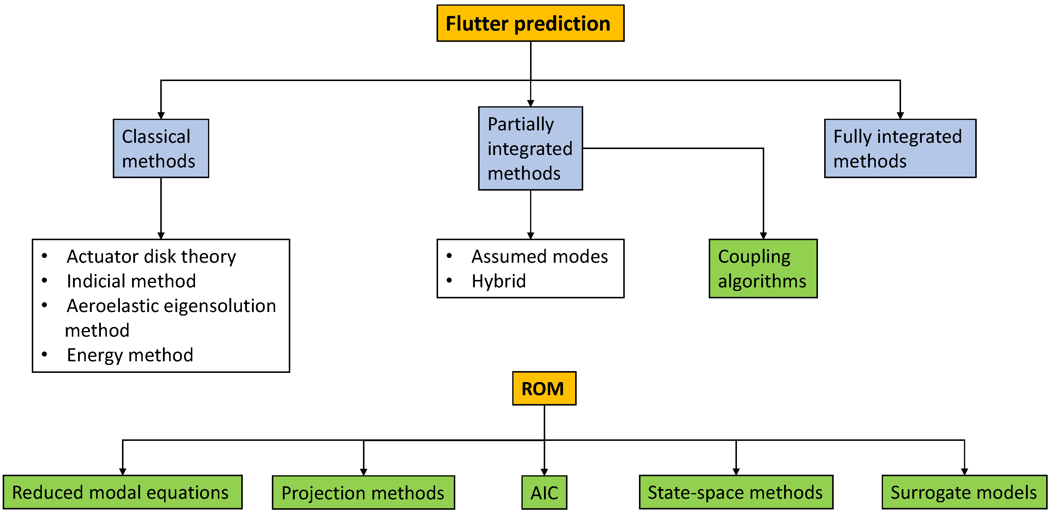
The main objective of the present paper is to review computational methods for flutter prediction, focusing on aspects such as methodology, complexity, fidelity to physical phenomena and accuracy, computational requirements, applicability to design and analytic purposes. The last systematic review in the field was carried out by Marshall and Imregun in 1996 [2]; in our work, a synthesis of legacy methods from a modern point of view and their applications in the literature is proposed. The progress made from the previous review in terms of techniques and computational expenditures involved is also highlighted, and the new state of the art in flutter modelling is depicted. Another treated topic is the sum of techniques employed to reduce the computational cost of aeroelastic models, known as reduced order models (ROM); an overview is provided on mathematical formulations, applications, expected accuracy and limitations. A schematic of this paper is presented in Figure 1; after a brief presentation of CFD methods for turbomachinery unsteady flow calculations, the most widely adopted techniques to numerically model flutter throughout the years are described, distinguishing between classical methods and coupled ones. Two insights are made: one on coupling algorithms and the other on model order reduction to decrease computational cost.
2. CFD Methods for Unsteady Flows in Turbomachinery
The dramatic increase in the computing power and the advances in CFD methods have drastically enhanced the complexity and fidelity of computational models for flutter predictions in turbomachinery. Early studies on unsteady flow modelling involved the use of full-potential or Euler equations, where the hypotheses of inviscid, compressible and rotational flows were adopted. Both methods were used to calculate time-dependent inviscid flows when the unsteady terms are discretized to the desired order of accuracy. However, the full solution to the equations was expensive, so that linearization—whereby each variable is expressed as a mean value plus a small perturbation about that value—was adopted [3,4]. The applicability to turbomachinery flutter simulation is questionable, since linearization prevents an accurate treatment of transonic flows and the capturing of limit-cycle behaviour. However, when the prediction is focused on the flutter onset only, the linearization hypothesis is often realistic. Natural developments were non-linear potential and Euler methods, where no linearization is made during the unsteady calculations. Boundary layer effects were often included using a technique known as viscous–inviscid interaction, where regions far from the structure are modelled as inviscid and extra equations are needed to account for turbulence near the wall structure [5]. Other forms of boundary layer treatment employed heuristic methods to account for viscous effects and shear stresses [6].
Today, the compressible and fully viscous Reynolds-averaged Navier–Stokes (RANS) equations are the state of the art in CFD modelling, the only simplification being the time averaging of turbulence quantities using one to six equation models [7]. Thanks to recent improvements in available computing resources, this technique is now frequently adopted to model unsteady 3D flows spanning multiple passages or even the full bladed annulus, with multiple million node meshes [8,9]. Recent further developments involve the employment of large eddy simulations (LES) or detached eddy simulations (DES) [10], where the larger eddies are directly modelled, and the smaller treated with RANS. LES methods have the potential to reduce errors in computing flow regions having non negligible viscous blockage, where current turbulence treatments are inadequate, and could possibly predict separation phenomena in stalled conditions more accurately, but they still exceed the typical computing power available in routine calculations.
Time integration with different discretization algorithms still constitutes the benchmark in unsteady flow modelling; however, time-accurate nonlinear models can be very expensive, even for modern computers. For this reason, and because of the inherent spatial periodicity of turbomachinery passages, solvers developed in the frequency domain have gained an increasing interest. A recent promising development is the harmonic balance (HB) technique, proposed by He et al. in [11]. Using this approach, the unsteady flow is assumed to be temporally and spatially periodic, a condition satisfied with good approximation for many unsteady flows of practical interest. In his original approach, Hall [12] represented periodic unsteady flows by a Fourier series in time with frequencies which were integer multiples of the original excitation frequency. The dependent variables were the coefficients of the Fourier series for each of the conservation variables. These Fourier series were then inserted into the Euler equations, the resulting expressions were expanded and terms were collected frequency by frequency. For the Euler equations to be satisfied, each frequency component must vanish independently. The result is a set of coupled complex partial differential equations, one for each frequency retained in the model. Because time does not appear explicitly, the harmonic balance equations can be solved as steady-state flow problems. To increase accuracy and stability in treating the more complex Navier–Stokes equations, Hall et al. [13] developed an improved version of the harmonic balance technique in which the dependent variables are the conservation variables stored at a number of subtime levels over one period. This approach proved to be suitable in modelling flows with excitations which are non-multiple of a single frequency (i.e., blade flutter with forced response from neighbouring blade row wakes) [14]. The computational cost of harmonic balance depends on the number of subtime levels adopted and frequencies retained and is typically more than one order lower than unsteady simulations, with a comparable level of accuracy [13]. The method was adopted in the works by Aschcroft [15]; Sicot [16]; Ekici [14], who studied a 2D compressor stage subjected to flutter and forced response; and Berthold [17], who adopted HB to solve both nonlinear structural and fluid equations in a coupled algorithm.
3. Aeroelasticity Methods in Turbomachinery
The aim of aeroelastic methods for flutter prediction in turbomachinery is to solve the generic motion Equation:
where x is the vector containing physical coordinates of the structural model degrees of freedom (d.o.f.); M, D and K are the mass, damping and stiffness matrices; and is the time-dependent vector of aerodynamic forces acting on degrees of freedom at the domain interfaces. When different effects are included, such as nonlinear forces due to friction dampers, the related terms are usually added to aerodynamic forces. Computational approaches to model flutter in turbomachinery could be divided into two broad categories: classical and integrated methods, the former ignoring the interaction between the fluid and the structure, and the latter attempting to model it.
3.1. Classical Methods
Classical aeroelasticity methods are those where the fluid and structural domains are uncoupled, so that the fluid flow does not affect the structural response which is pre-determined. Such methods thus split an inherently coupled nonlinear phenomenon into two separate uncoupled analyses.
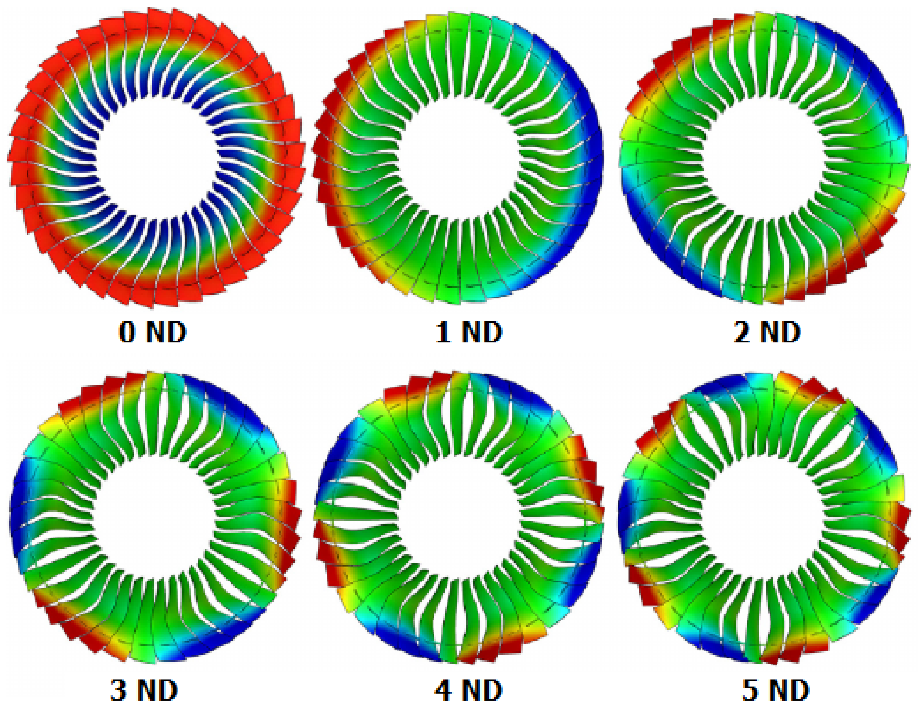
One of the key concepts in turbomachinery aeroelasticity, introduced by Lane [18], is the interblade phase angle (IBPA): the individual blades in a cascade are assumed to vibrate with the same amplitude and mode shape, but the maximum is reached with a constant phase lag, known as IBPA. With non-zero IBPAs, the cascade is assumed to vibrate in the so-called travelling wave mode, whereas a zero IBPA implies a constant phase between all blade displacements and a standing wave pattern. Figure 2 provides a visual representation of different nodal diameters (ND) in a vibrating bladed disk, where colours indicate blade displacements. IBPA is related to the number of NDs (diameters of the disk where blade displacements are zero) according to the Equation
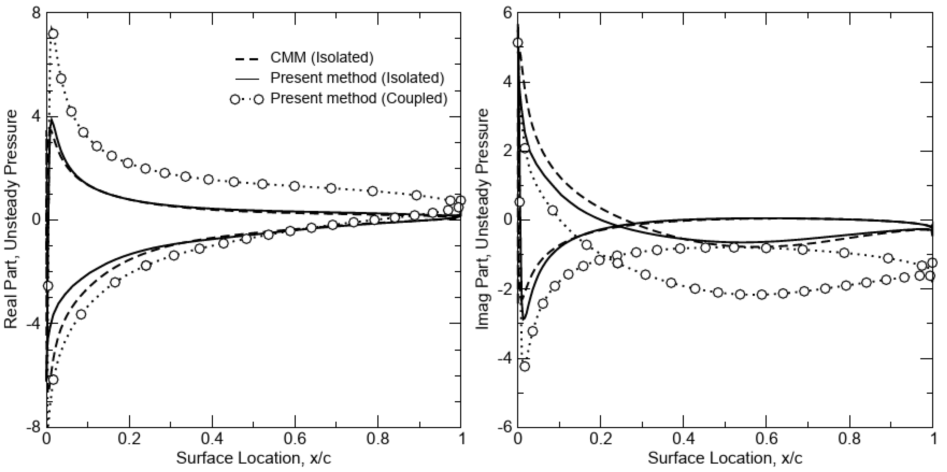
In classical methods, the structure and the fluid are decoupled so that a free vibration problem can be solved first. Normal mode-shapes and frequencies can either be calculated in a free vibration problem (in vacuum) or taking into account gyroscopic effects, centrifugal stiffening and steady airloads of a given operative condition. Then, the predicted mode-shapes are used with an arbitrary amplitude to calculate the unsteady aerodynamic forces, from which a measure of stability is inferred. Typical outputs of classical imposed-oscillation analysis include real and imaginary components of pressure distribution on blades’ surfaces, as shown in Figure 3. Different formulations of classical methods have attained high popularity thanks to three main factors:
- Simplicity of models and relatively low computational costs, due to lack of interexchanging information between the two domains at each substep.
- The assumption of uncoupling between the fluid and structural domain is usually realistic for many situations, especially at low speeds, so that the motion of the structure is well defined by a certain mode shape and frequency, which are substantially unaffected by the unsteady flow.
- The information regarding asymptotic stability of given modes and IBPAs, though conservative, is sufficient in many cases, especially for preliminary design purposes.
The main drawback of this method is the inherent simplification of flow nature given by the linearisation of unsteady flows, especially true when nonlinear phenomena such as shock waves are present and the mass ratio is low. A common way to partially circumvent this aspect is achieved by varying the prescribed (small) oscillation amplitude and assessing the linearity of flow response on the blades. Another direct consequence of uncoupling is the inability to predict limit cycle behaviour in blade oscillation patterns, which could prevent a complete understanding of the blade behaviour under actual loading conditions.
3.1.1. Actuator Disk Theory
Actuator disk representations are simplified forms of linearized cascade theories, based on the fundamental assumptions of low reduced frequency and small interblade phase angle (Whitehead [19]). Tanida and Okazaki [20] developed a variant where the hypothesis of small frequencies was relaxed, and the method was improved to be used with 2D compressible flows by Adamczyc [21]. The actuator disk model calculated the unsteady aerodynamic forces as a function of the steady flow field and the dynamic response of the cascade. Linearized potential equations were generally adopted, and viscous and stalling effects were included via experimentally derived quasi-steady loss coefficients. In principle, different viscous loss coefficients should be derived for each new geometry; however, it was not uncommon to use the original coefficients for a wide range of blades. The main limitation is that the method requires ‘tuning’ to each particular type of problem, and its performance would be poorer where viscous effects are known to be important, such as in transonic stall flutter. The early version of actuator disk theory, as developed by Whitehead, could not properly simulate non-zero IBPA and used the assumption of infinitesimal chord length and spacing, so that flutter boundaries in strictly limited conditions could be computed. Later methods such as the one by Adamczyc adopted compressible transonic flows and quasi-steady total pressure loss coefficients to predict flutter boundaries of four high-speed rotors, with slightly conservative results. The steep variation in viscous forces associated with a rapid rise in the tip blade-element was identified as the cause of flutter onset.
3.1.2. Indicial Method
The indicial method was proposed by Ballhaus and Goorjian [22] and further explored by Ueda and Dowell [23] and Stark [24]. It used transonic small disturbances (TSD) or linearized potential equations to compute the unsteady forces acting on an airfoil in transonic flow. The flow response due to a step-change in the airfoil position was computed first, and the response to any other prescribed motion was obtained via the convolution integral from this initial result. The cascade motion was assumed to be simple harmonic, so that the aeroelastic equations of motion could be solved by standard matrix techniques once the aerodynamic forcing terms were known. The indicial method by Ueda and Dowell proved suitable in predicting flutter boundaries of two-dimensional pitching cascades in a wide range of reduced frequencies with a very small amount of computation time compared to time-marching solutions. The method was capable of predicting nonlinear limit cycle flutter confirmed by time-marched simulations, but generally, the accuracy of the describing function method decreased as the amplitude of the motion increased. Moreover, the neglection of the component in the upwash distribution due to the angular velocity of the airfoil motion caused a fictitious flutter instability at high frequencies. However, the use of convolution integrals and excitation signals presents the advantage of predicting the flutter boundary over a range of conditions from only one set of time-marching fluid calculations. It is also the basis of another method named aerodynamic influence coefficients, frequently adopted as a ROM and described later on in the paper.
3.1.3. Aeroelastic Eigensolution Method
This method is based on obtaining the linearized harmonic unsteady aerodynamic coefficients for the motion of a freely vibrating structure. The unsteady aerodynamics can be provided by anything from empirically determined airfoil lift and moment coefficients, through linearized potential methods, to nonlinear RANS codes. The structural model is usually represented as a two-degree-of-freedom section, but the formulation is general, so that 3D blade descriptions can also be accommodated. Once determined, the aeroelastic forces are expressed in the frequency domain, either directly if analytical theories are used or by Fourier analysis if the forces were first calculated in the time domain. The resulting aeroelastic equations of motion are obtained by adding the aerodynamic contributions to the mass and/or stiffness matrices of the structural equation. However, these new system matrices may well become a function of the frequency, in which case, the eigenproblem is no longer linear. In such situations, an approximate solution can be found using iterative techniques. The stability of the system is then assessed by considering the amount of damping in each aeroelastic mode. Many applications of the methods can be found in the open literature, among those [25,26,27]. Early models employing the aeroelastic eigensolution method used potential linearized CFD codes, computing the airloads as a linear function of the blade displacement and assuming the superposition of effect due to different modes. The flutter boundaries obtained are essentially qualitative; nevertheless, the dependency of vibration eigenmodes on airloads and a resonance at nominal speed for an experimental fan was captured by Klose [25]. More advanced techniques employing multiple-passage domains often rely on the assumption of airloads which are linearly dependent to blade displacement and velocity. The model of Tateishi [27] correctly predicted flutter boundaries in a range of conditions except low speed lines, where the effect of grid size and the accurate simulation of shock impingement appear to be critical factors.
3.1.4. Energy Method
The energy method, first developed by Carta [28], is based on calculating the sum of the work done by unsteady aerodynamic forces on blades, which oscillate with a prescribed motion of pitching or plunging (2D sections), or determined from a free-vibration analysis (when 3D models are used). It is inherently assumed that the flutter behaviour is linear: positive aerodynamic work, i.e., energy transfer to the structure, indicates instability, while a stable situation is characterized by a negative net aerodynamic work. The aerodynamic damping is defined as the work of aerodynamic forces on blades over a cycle W, usually normalized with respect to the blade vibration mechanical energy , as indicated in Equation (3).
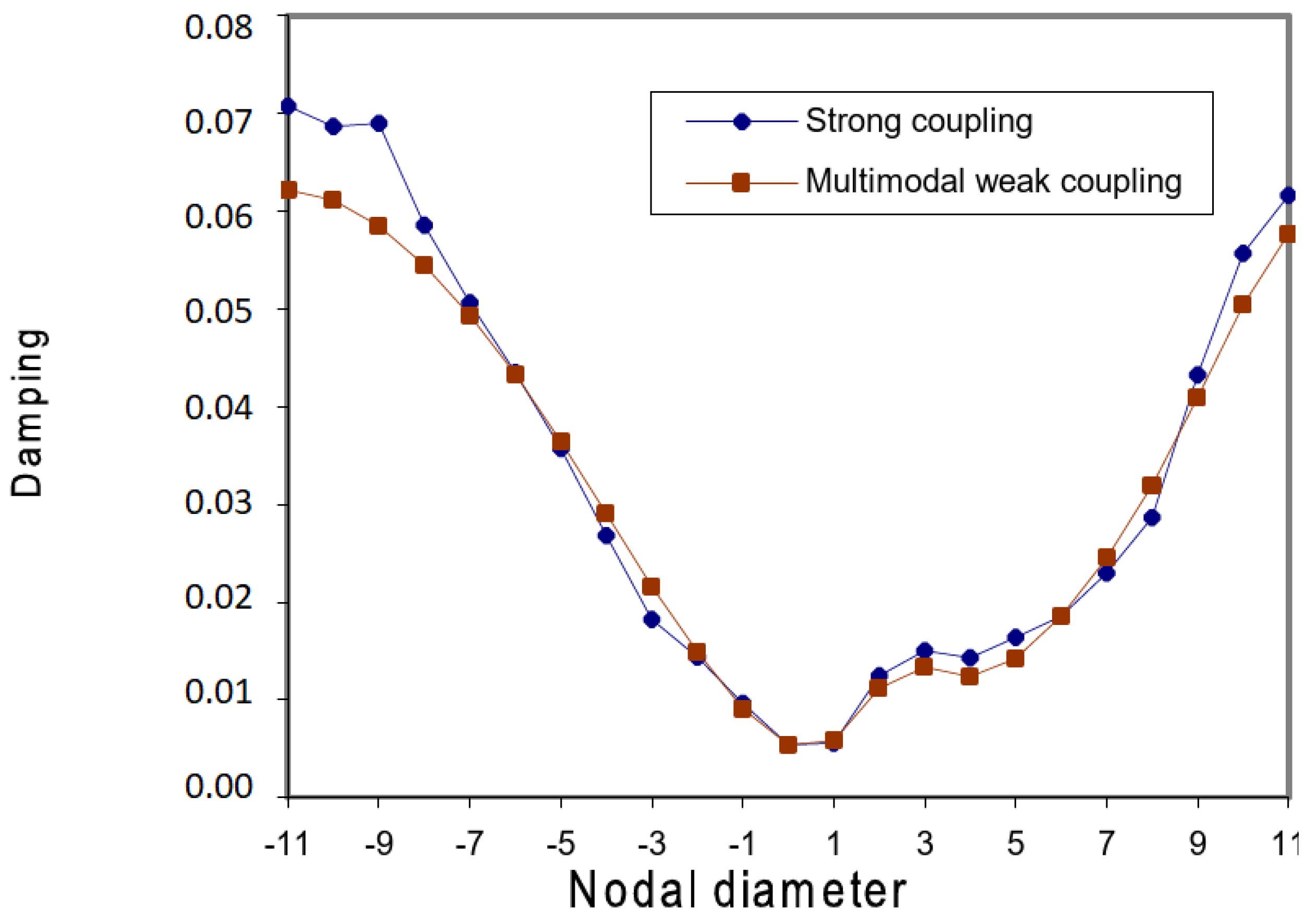
The stability of the bladed disk is assessed by calculating the aerodynamic damping for each IBPA for every single mode-shape oscillating at its natural frequency, as shown in Figure 4, from Mahler [26]. The method was historically implemented calculating the work per unit of a span on a number of 2D sections, using linearised aerodynamic theories. The process of assessing the overall stability by performing this worksum procedure was found to be ill-conditioned, the result being indicated by a small number, obtained as the algebraic sum of large numbers; the accuracy of the calculated damping was thus largely affected by the number of sections chosen. Today, with more computational power available, this approach and its many variants are implemented with 3D simulations and represent the state of the art in turbomachinery flutter analysis in the aerospace industry because of their simplicity. However, the fluid and structure domains are still treated as two separate media; thus, considerations and limitations of classical methods hold true. Examples of energy method applications are found in many works, including simulations of stall flutter and flows with large, separated regions, e.g., in [29]. The method is also used to compare the accuracy of coupled methods to well-known uncoupled formulations, as in [26,30,31,32,33]. Figure 5, taken from Mahler [26], plots aerodynamic damping versus IBPA for two different coupling algorithms.
3.2. Integrated Aeroelasticity Methods
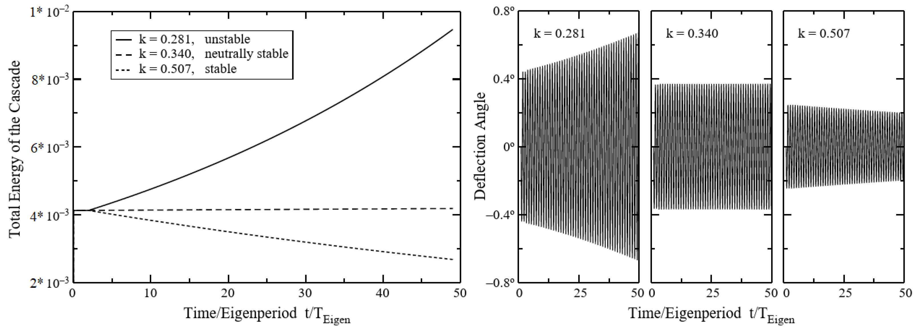
Integrated aeroelasticity methods are those which do not uncouple the flow motion from that of the structure but attempt to treat the problem in one continuous medium [2]. The need for such an approach arises from the inherent nonlinear behaviour of unsteady high-speed viscous fluid flows, especially when shock waves and separation phenomena are considered, e.g., in transonic flutter or in stalled conditions. The existence of nonlinear structural effects such as friction damping in the blade roots and shroud interfaces further justifies the implementation of such methods. The mathematical formulation of integrated methods is devised in such a way that the flow behaviour is allowed to modify the structural motion, and vice versa, as in the true physical phenomenon. The most striking difference between the classical methods and integrated ones is that the former can only predict the onset of flutter as a sudden change from a stable to an unstable region, while the latter are capable of predicting limit-cycle behaviour, a constant amplitude oscillation due to nonlinear aerodynamic phenomena, as shown in Figure 6. Experimental evidence suggests that flutter can occur at different limit cycle amplitudes influenced by both aerodynamics and structural damping, and the prediction of that amplitude is crucial in assessing the life of turbomachinery components. Integrated algorithms can also predict nonlinear instabilities, i.e., situations where the equilibrium point is locally stable, but for sufficiently strong perturbation, the frictional dissipation cannot bound the flutter vibrations, as proved by Berthold [17]. As with classical flutter analysis methods, different formulations are possible for the integrated methods: one key factor in categorizing different algorithms is the numerical treatment of the physical domains (i.e., whether fluid and structure are discretized into a single domain or not). Another parameter is the accuracy in assessing fluid–structure equilibrium at each physical timestep in time-marching simulations.
3.2.1. Partially Integrated Method
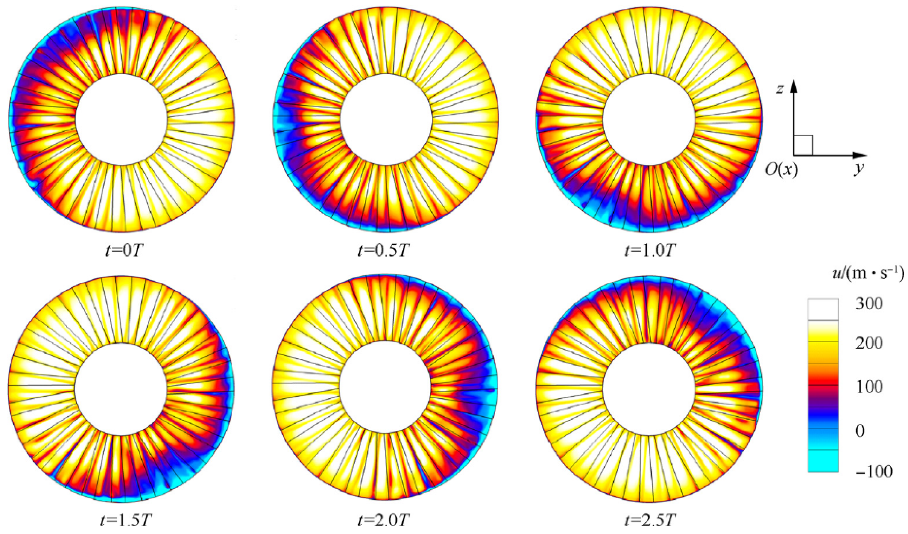
In the partially integrated methods, the solutions of the fluid and structural equations are calculated separately, but the information is exchanged at each time step, so that the solution from one domain is used as a boundary condition for the other domain. In other words, a new blade position is calculated at each time step using the fluid forces of the previous time step, and this new position is used as the new fluid–structure boundary for the next time step when the aerodynamic forces are computed first. Many examples of partially integrated methods can be found in the open literature. In the works by Sayma [34], Sadeghi [31], Debrabandere [35], Zheng [36] and Li [37], the eigenmodes were computed using constant or Rayleigh structural damping model, and the domain was reduced to one or two passages to contain the computational effort, with a limitation on the explorable IBPA range as a payoff. Coupled simulations showed that the normal ’in-vacuum’ eigenmodes can be significantly different from the aeroelastic mode, especially at low mass ratios, leading to inaccurate results when assumed modes and the energy method are employed, as evidenced in Figure 7. Furthermore, a nonlinear fluid–structure interaction can lead to the oscillation of blades around a displaced position, with two different harmonics and a pattern of alternated chocked and unchocked flows in neighbouring passages, as evidenced by Sadeghi [31]. Fluid–structure coupling also permits the simulation of a forced response [35]; the influence of the passing rotor on stator blades is captured, and the Fourier transformation of induced vibrations showed that they are more related to the natural stator frequencies than to the rotor passing frequency. Various works adopted multiple mode superposition in coupled simulations, but some evidence suggested that the influence of modes next to the first is often negligible. In the papers by Liang [38] and Zhang [39], the structural reduction to a few modes (including centrifugal stiffening and the Coriolis effect) was coupled to the three-dimensional full annulus fluid model of transonic compressors, relaxing the limitations on permitted IBPA and allowing the simulation of complex phenomena such as rotating stall and nonsynchronized vibrations. The computational model of Liang [38] showed that rotating stall cells have about 30% the rotor speed (see Figure 8) and an energy mainly distributed in the first two orders of excitation. Some resonances were found between blade modes and the stalled flow cell velocity; a novel algorithm was built to predict those resonances. In the paper by Zhang [39], the rotating stall was simulated showing a limit-cycle oscillation of all blades as the stall line was approached, followed by flutter as the system became dynamically unstable, with all the blades vibrating at the same mode and frequency but with different amplitudes. A sinusoidal travelling wave pulsation was observed during flutter, but with a non-constant IBPA. Im [10] simulated flutter for the NASA Rotor 67 at different operative conditions using a fully coupled partially integrated model with both a four-passage domain and the full annulus, showing comparable results for the two cases in unstalled flutter conditions.
3.2.2. Periodic Mode Updating Method
This method is a hybrid between classical and partially integrated aeroelasticity methods. Similar to the aeroelastic eigensolution method, a free vibration problem is solved in the frequency domain, and the mode shape of interest is used to describe the blade motion for one period using a 3D time-marching nonlinear CFD code. After the first period is simulated, the mode shape is updated using aerodynamic coefficients which were calculated in the previous period, via a frequency-domain structural calculation based on modal projection. The cycle of time-domain aerodynamics, followed by frequency-domain structural dynamics, is repeated until the mode calculated in the frequency domain converges. An example of such a procedure can be found in the work of Gerolymos [40]. The model adopted a rather coarse mesh and was used for illustrative purposes. It was found that the coupling slightly affected the mean accumulated power on blades, but this difference was sufficient to lower the aerodynamic damping by 30%.
3.2.3. Fluid–Structure Coupling Algorithms
Since each of the components of the coupled aeroelastic problem has different mathematical and numerical properties, well-established but distinct numerical solvers and readily available commercial software, the simultaneous solution of the equations by a monolithic scheme is, in general, computationally challenging, mathematically and economically suboptimal and unmanageable software-wise. On the other hand, the solution of the aeromechanical system through different integration schemes and the exchange of information between the two domains presents various issues and requires some precautions.
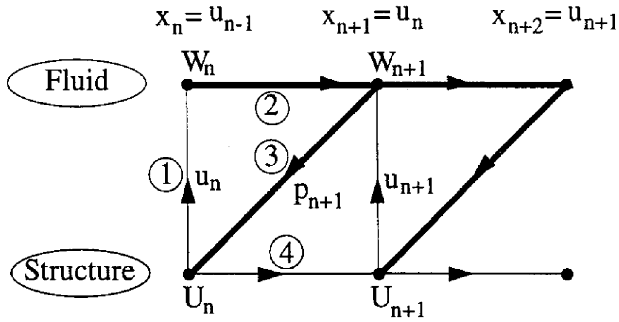
The simplest form of the integration algorithm is depicted in Figure 9. The flow solver is advanced for one physical time step, then the fluid load is sent to the structural solver that computes the corresponding deformation and a new iteration starts. As the equilibrium between the structure and the fluid is not ensured at the end of each iteration, this is called a weak-coupling method. Examples of weakly coupled algorithms can be found in [34,35]. More accurate representations of fluid–structure interactions ensure the equilibrium of quantities such as force, displacement and energy at each physical substep by subiterating the governing equations until the prescribed tolerance on the chosen quantities is reached: those methods are named fully coupled and were adopted in [10,31,37,38,39].
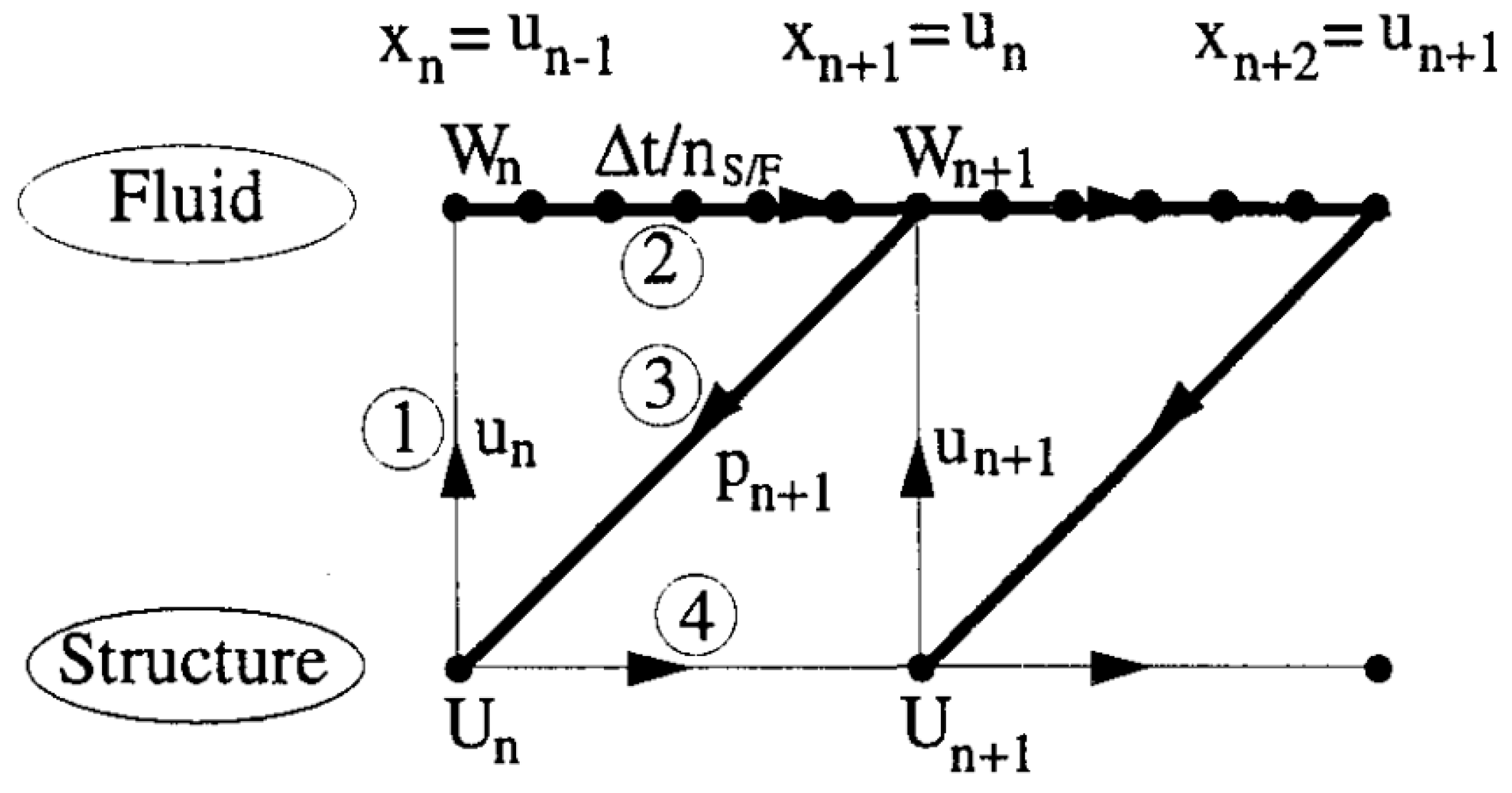
Since the typical time integration steps needed for accuracy and stability reasons may differ by orders of magnitude between the structural and fluid problem, in almost all aeroelastic problems, it is the integration of the fluid state vector that requires a much finer temporal resolution than the structural vibration. For this reason, some algorithms were developed that subiterate the fluid flow with a factor equal to the structural/fluid timestep ratio, reducing the needed advancements of the structural domain and I/O transfers, as shown in Figure 10. However, in certain cases, the cost of subiterations can offset the benefits of the larger timestep they can allow.
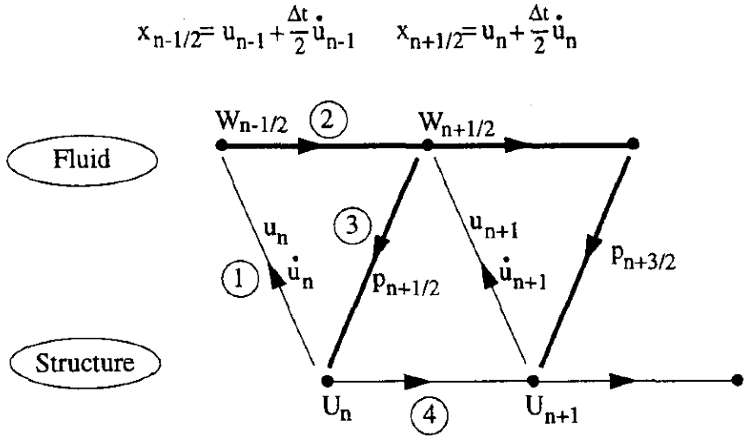
More advanced methods try to achieve an accuracy comparable to that of a monolithic or fully coupled scheme but with a reduced computational cost: among these are the displacement and velocity conserving staggered algorithm by Farhat and Lesoinne [41] and employed by Carstens [42]. As schematized in Figure 11, the computations of structural displacements and fluid state vectors are shifted by , while the CFD-mesh deflections at the blades’ surfaces are calculated from the structural displacements. Furthermore, the mesh deformation is computed by Newmark’s algorithm estimating the constant acceleration in the time interval from the unsteady aerodynamic forces at time .
3.3. Fully Integrated Methods
Fully integrated methods differ from their partially integrated counterparts in the discretization and subsequent numerical treatment of the governing equations. They are based on formulating the structural and fluid dynamics together so that they can be solved at each time step using the same integrator. The two domains are discretized into one arbitrary Lagrangian–Eulerian (ALE) space; as a consequence, the motion of the grid becomes an integral part of the equations of motion and does not have to be handled separately. The direct method uses an explicit temporal discretization which is integrated using a Runge–Kutta scheme, and upwind differencing is used for the spatial discretization of the arbitrary Lagrangian–Eulerian formulation of the aeroelasticity equations. The structural equations are formulated on a local nodal level, which enables them to be discretized using the same integrator as the aerodynamics. Thus, both sets of equations are handled simultaneously at the same time step without distinguishing between the fluid and the structure. This model is claimed to calculate the energy transfer between the structure and the fluid more accurately than similar partially integrated schemes since there is no possibility of a time lag between the structure and the fluid. The method was developed by Bendiksen [43] and applied to both wing and cascade flutter using quasi three-dimensional models, predicting divergent behaviours and limiting cycle flutter in a range of conditions.
4. ROMs for Flutter Prediction
Reduced order models, or ROM, elicited great interest in the past because of the limited computing power required compared to high-fidelity CFD. However, their use of simplified fluid flow models carrying strong and restricted hypotheses inevitably led to inaccurate or mere qualitative calculations in many cases. Currently, viscous RANS models are commonly used in turbomachinery modelling thanks to an increased available computing power, thus allowing for a significant reduction in the effort needed to model multiple blade passages. However, the accurate treatment of non-axisymmetric problems, such as inlet-distorted cases, rotating stall cells and non-synchronous vibrations, and the modelling of coupled fluid–structure interactions still entail dramatic computational costs due to the necessity of full-annulus domains and complex coupling algorithms. For these reasons, reduced order models still remain attractive for a variety of complex applications, where computational power saving leads to viable industrial uses, as long as the choice of restraining hypotheses adopted does not excessively affect physical consistency and fidelity. In this section, techniques to reduce the computational cost of flow and structural modelling in turbomachinery flutter simulations are presented.
4.1. Reduced Modal Equations
In the reduced modes methods, the structural model is computed from a finite element analysis of the structure; it can be determined from experimental modal analysis (system identification), Rayleigh–Ritz methods or, more frequently, using the finite-element method. Equation (1) is decoupled using the normalized mode shapes relation:
and premultiplying Equation (1) by , the system becomes
Usually, the mode shapes are normalized with respect to the mass matrix
In this way, j decoupled equations are obtained in the form
Only the independent (or orthogonal) modes of interest (usually from one to five) are retained in the problem, the higher modes being considered to be beyond the frequency range at which flutter is expected to occur. The response of the structure is calculated as the superposition of orthogonal modes by means of the so-called modal summation technique. The solution to the aeroelastic equations of motion is usually sought in the time domain with constant diagonal mass, stiffness and damping matrices, which are expressed in principal coordinates so that the structural part can be dealt with in the most efficient manner. Additional terms such as centrifugal stiffening or spin softening can be included in the stiffness matrix, while the Coriolis force can be placed in the damping matrix; however, it should be pointed out that the latter two effects are often negligible. Structural damping is often treated using the Rayleigh model, with terms proportional to mass and stiffness matrices. When the nonlinear effect of friction dampers is included, the related terms are usually summed to the aerodynamic forcing vectors on the right-hand-side of Equation (1), and a solution is searched for iteratively [34]. The dependent variables in the aeroelastic equations of motion then become the modal variables rather than the spatial variables. The aerodynamic pressure loads, at the right-hand-side of the equation of motion, are projected on the modal coordinates as well. The mapping usually takes place at the start of the computation and not at each time step, a feature which reduces the computational effort further.
While some studies have adopted full finite elements methods (FEM) to study static aeroelasticity in external flows, there is little evidence that a similar approach could provide more accurate results in turbomachinery applications without considerably higher expenses in computational cost. Thus, the reduction of the structural model to only a few modes is the routine practice in turbomachinery flutter calculations. Since there is an exchange of information between the structure and the fluid, the model can be used to predict limit cycle behaviours and divergence, the computing power required being dictated by the CFD technique employed.
4.2. Projection Methods
The key points in “projection methods” ROMs, as pointed out by Willcox [44], are the following:
- A small number of solutions using the full model are computed. The conditions for these full solutions or “snapshots” are chosen to span the operating range over which fidelity to the CFD results is desired.
- A set of basis vectors which capture the behaviour in the solutions is created. “Behaviour” can be quantified by spatial patterns in the flow, snapshots of the unsteady response (frequency domain) or the input–output transfer functions. The number of basis vectors required depends on the problem and the desired degree of fit.
- The original equations are projected onto the space represented by the basis vectors. The result is a set of ordinary differential equations (ODEs) for the time-varying coefficients of the basis vectors. The low-order system is completely defined by these coefficients or “states”; an approximate reconstruction of the entire flow field can be accomplished by multiplying the states by the basis vectors. Thus, any output quantity (blade pressure distribution, downstream disturbances, forces and moments) can be approximated.
A commonly used projection technique is the proper orthogonal decomposition (POD), originally devised for signal analysis. The original unsteady flow field is first decomposed in a steady mean component and in a fluctuating part. The technique is based on the decomposition of the fluctuating field in orthogonal components; eigenvectors of the signal autocorrelation matrix become the temporal coefficients , while the projection of the original signal on those coefficients originates the spatial modes . The eigenvalue associated to each eigenvector represents the mode energy. The fluctuating signal is reconstructed as a summation of temporal coefficients multiplied by the spatial modes and weighted by the autocorrelation matrix eigenvalues (Equation (8)). Usually, a number of around five modes is sufficient to catch more than 99% of the flow energy.
In temporal “snapshot” POD, the eigenvectors are obtained by solving the eigenvalue problem in Equation (9), where R is the autocorrelation matrix of signal snapshots, obtained through the internal product (Equation (10)).
A different version of POD for fluid flow reconstruction calculates the eigenmodes from a harmonic correlation matrix, formed using the Fourier coefficients of chosen variables at grid points. POD methods are also employed to reduce spaces spanned by parameters different from time or frequency, becoming suitable tools for optimizations or inverse design problems [45,46]. The main advantage of POD techniques resides in shifting the computational expense in the snapshots calculations, while the ROM usually takes seconds to compute a given flow condition. The main drawbacks lie in the hypothesis of small perturbations, linearity and orthogonality of modes, which can affect highly nonlinear flow reconstruction. Particular care should also be taken in choosing a sufficient number of snapshots to describe the case of interest.
Epureanu [47] used a coupled viscous–inviscid interaction model for the flow computation over an oscillating cascade. The snapshot POD technique in the frequency domain was adopted to build a ROM spanning a range of frequencies and IBPA. The model with only 25 d.o.f. provided accurate results over a wide range of reduced frequencies, comparable to those of the full model with 10,000 d.o.f. In [48], the author adopted the same method to a transonic case, evidencing the need for a higher number of modes (55) to accurately model shocks, while the influence of reduced Mach number seemed to be negligible. Willcox in [49] adopted a POD-based reduced order model to describe the vibration of a 2D compressor cascade with 2 d.o.f. in a range of reduced frequencies and IBPAs. The first order expansion of the unsteady flow, with separate components due to pitching and plunging motion, was substituted in the governing linearised Euler equations, and using orthogonality, a system of ordinary differential equations for the modal coefficients was obtained. That system was coupled with a structural model, transformed in state-space form and solved in the time domain. In [50], the author used a similar approach based on the Arnoldi vector for the ROM construction. Clark in [51] used POD to model non-synchronous vibrations over a 2D oscillating cylinder and a compressor cascade. The unsteady RANS equations were solved in the frequency domain adopting the harmonic balance method. A POD analysis was performed on the harmonic coefficients, and a ROM was built including a small number of modes for each condition simulated. A number of states, varying the oscillation amplitude and the Strouhal number, were simulated, and a high-order polynomial response surface was adopted to fit mode coefficients and create a predictive tool. A modal assurance criterion was used to assess predicted CFD solution accuracies, and a strong improvement was achieved by taking into account the generalised blade force in the prediction model. In [52], Sarkar adopted the eigenmode-based system equivalent reduction expansion process (SEREP), in which a state-space model is reduced by retaining the most significant eigenmodes. The CFD code solved the two-dimensional vortex lattice equations over an oscillating NACA0012 airfoils cascade; after selecting the number of modes to be retained, a transformation matrix was built up, which maintained the same eigenvalues as the original system with few retained modes. The technique was compared to POD, showing comparable accuracy with lower computational effort.
4.3. Aerodynamic Influence Coefficients
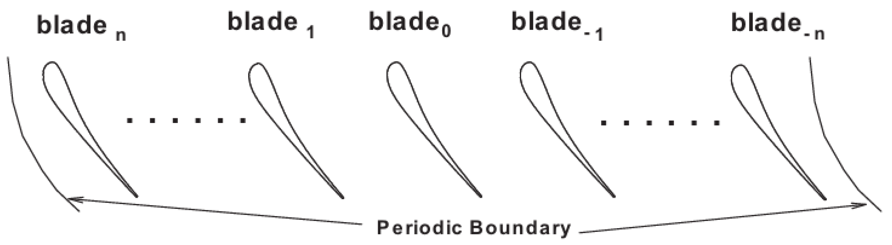
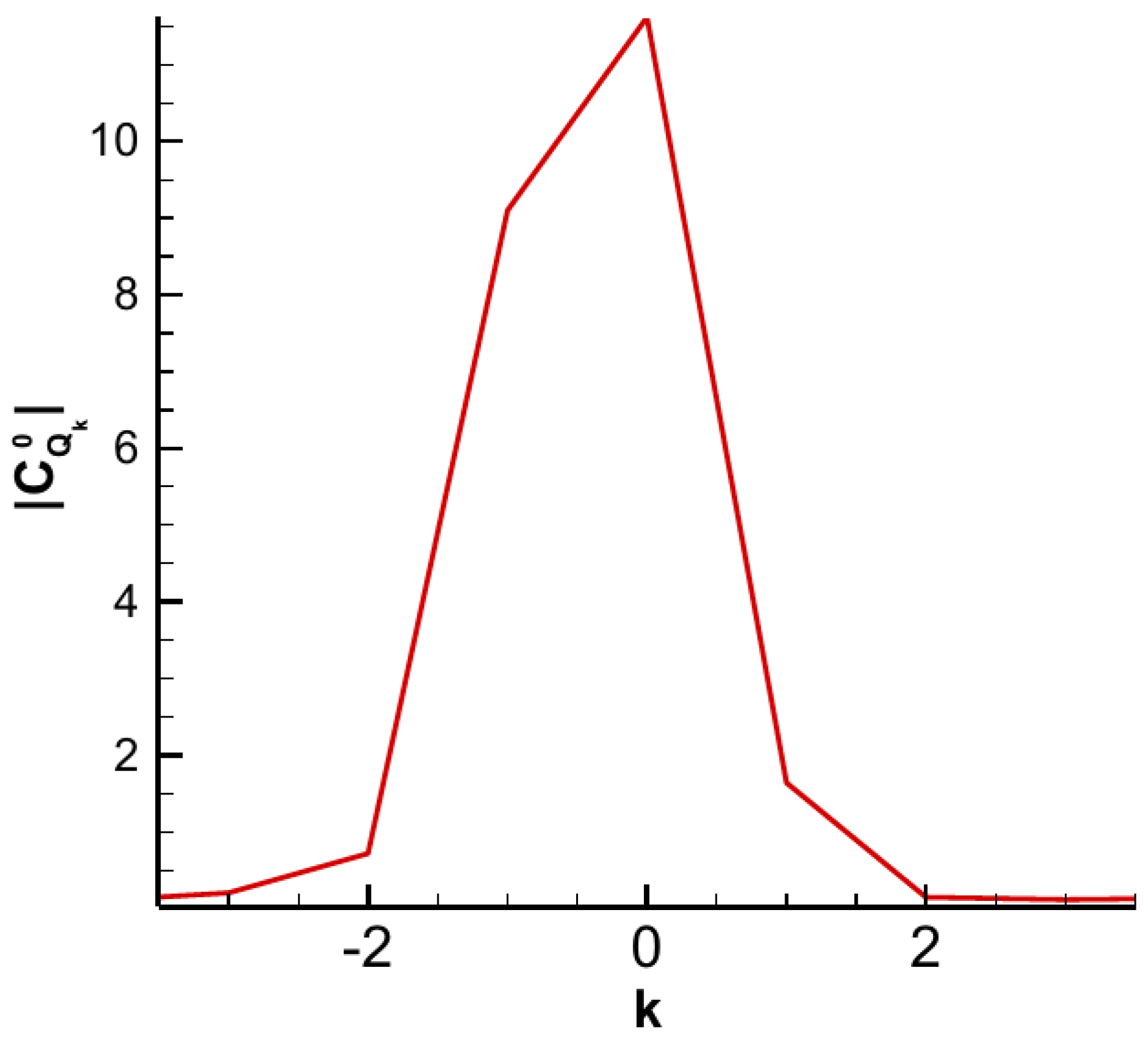
Another important technique for model order reduction in turbomachinery involves the employment of aerodynamic influence coefficients (AIC). Firstly developed by Hanamura [53], the method is based on the assumptions of small perturbations, linearity and superposition of effects and on the experimental evidence that disturbances emanating from the vibration of one blade are limited to an area of a few neighbouring passages and quickly decay over distance. A domain comprising 2N + 1 blades as in Figure 12 is numerically simulated or experimentally tested: the central blade harmonically vibrates with a prescribed motion, and its influence in terms of unsteady pressure is registered on the neighbouring stationary 2N blades. The unsteady loads can be expressed as complex numbers through the Fourier transformation, as in Figure 13; the dynamic frequency-dependent characteristics can be obtained by a process of model training for a number of flow conditions. A full compressor model can be then constructed by computing each blade aerodynamic forces vector as the summation of neighbouring blade-induced AICs. The complex form of blade aerodynamic forces can be readily associated with a structural model and solved from a given initial condition through time-integration or in the frequency domain. Since, in principle, all blades are treated independently, this method is also suitable for mistuning modelling. As with many other reduction techniques, AICs adopt the linearity hypothesis and superposition of effects; nonetheless, their use has proven to yield accurate results in transonic cases too.
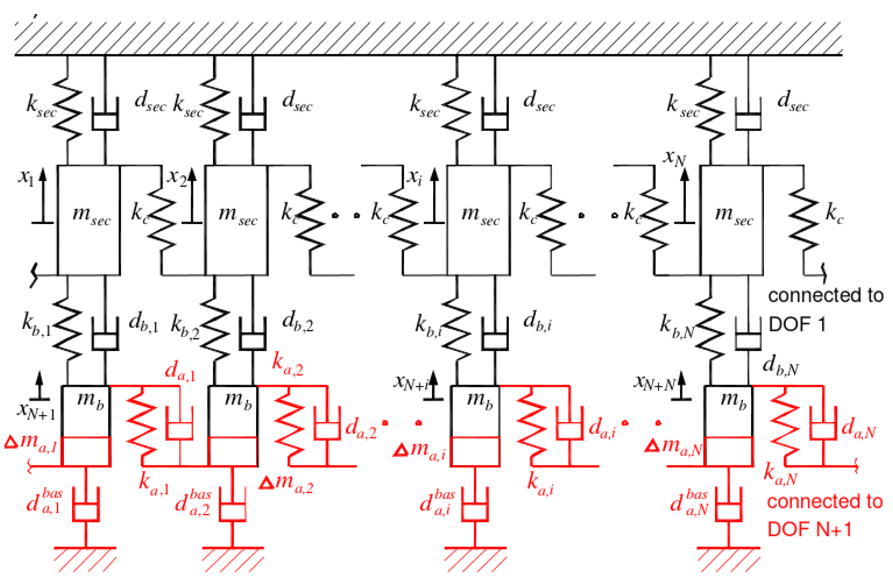
In the paper by Su [32], a single-input-multiple-output (SIMO) model was employed, and the dynamic response on each blade of the cascade was obtained by summing the AICs of neighbouring blades and taking advantage of the constant IBPA and travelling wave model. The method was implemented in both an uncoupled and coupled fashion by time-marching the structural equations with the complex form of pressure coefficients. In the work by Nipkau [54], the AIC model was used to construct the blade pressure distribution vector, and the system of equations comprising the structural model and the aerodynamic forcing terms was solved by calculating the aeroelastic eigenvalues: a method known as the equivalent blisk model (EBM). The aeroelastic eigenvalues were then used to derive the equivalent aerodynamic elements (EAE), schematized in Figure 14. These were the co-vibrating air-masses; discrete aerodynamic springs, to consider the stiffening or the softening affecting adjacent blades due to the flow; and aerodynamic dashpots. Both models were used in a forced response analysis considering mistuning, providing comparable results. In [55], Stapelfeldt simulated a 2D cascade using a form of AICs which accounted for vibration and vortical disturbances; the model was used to study the effect of mistuning on non-synchronous vibrations (NSVs) and stability with limited computational expense. In [33], Lian adopted a formulation of blade aerodynamic forces based on AIC to study NSV in a two-dimensional oscillating cascade considering mistuning. The AICs were calibrated by unsteady RANS computations with one oscillating blade and stationary neighbouring blades. The full model allowed mistuning by modifying single blade attenuation coefficients.
4.4. State-Space Representation
This method was first introduced for flutter control applications by Karpel [56]. The aeroelastic model consists of a set of structural modes and of airloads calculated using unsteady aerodynamic theories. The generalized aerodynamic forces are approximated using interpolation in the complex Laplace s-plane, the process being very similar to that used in the indicial method. The N second-order structural differential equations are reduced to 2N first-order differential equations, a transformation that leads to a first-order state-space model. This last set of equations can then be solved by the convolution integral. The success of the method largely depends on the validity of the linearity hypothesis for the unsteady flow description. When the order of the state-space matrix is very high, the balanced truncation method by Moore [57], using the controllability and observability of a linear system, could be adopted [10,58]: an example can be found in the work by Su [32], where an AIC-based SIMO model is changed into state-space form through a bilinear transformation and further reduced to be included in both coupled and uncoupled flutter models of a transonic rotor. Other examples where the state-space representation is used to solve a POD-based aeroelastic ROM can be found in the works of Willcox [44,49,50].
4.5. Surrogate Models for Aeroelastic Calculations
In performing model order reduction, many techniques lead to the calculation of flow field or blade aerodynamic forces in spaces spanned by different parameters (e.g., reduced frequency, reduced Mach number, etc.) but only at discrete points. Various strategies were thus adopted to estimate aerodamping parameters or to model the unsteady flow field in turbomachinery from discrete numerical or experimental data, using response surfaces or other surrogate models.
In [59], Rodriguez adopted a simple 3 d.o.f. mass-spring model to simulate turbine blade behaviour in flutter conditions with intentional mistuning, the aerodynamic forces being modelled from experimental data on aerodynamic damping. An asymptotic ROM was set up using a multiple scale method, exploiting the large difference between the elastic blade oscillation time and the long-time scale associated with the effects of aerodynamics, friction and mistuning. Tran, in [58], adopted a multi-parameter method to compute the generalised aerodynamic forces (GAF) on a large chord blade; the first harmonic of GAF Fourier coefficients was assumed to depend on blade displacement and velocity, and their values were computed at different sample conditions using the hypothesis of constant IBPA. A multi-parameter spline approximation of the GAF matrix was then used to build the reduced order coupled model; the minimum state smoothing method [56] provided a tool to reduce the model further in both frequency and time domain. The ROM obtained yielded the complex form of the GAF, suitable to be implemented in coupled computations. Using the extrapolation capability, both mono-parameter and multi-parameter minimum state modelling methods could predict unstable areas where the aerodynamic computations could not be achieved. In [60], Stel’makh presented a rapid method for predicting dynamic stability of compressor blade cascades and evaluating the critical dynamic stability loss conditions of direct compressor cascades. The method was based on a functional of angle of attack, cascade geometry, deflection angle, pitch-chord ratio, Mach number, blade frequency diversity and mechanical damping in the blade material and lock joints. The parameters were collected on experimental tests and used to build a database of critical reduced vibration frequencies.
A relatively new frontier in CFD ROMs is the use of polynomial response surfaces or artificial neural networks (ANN) to simulate the behaviour of flow response to various inputs. The main advantages prospected by the latter is the ability to treat nonlinear phenomena and the capability to emulate complex I/O functions when an appropriate number of layers and neurons are employed, the main limitations given by the relatively high training cost. In [61], Hu employed a recursive radial basis function neural network (RRBF NN) based on adaptive simulated annealing (ASA) to create a ROM for a cascade unsteady flow with dynamic inflow conditions. The model predicted dimensionless static and total pressure with respect to an arbitrary dynamic incidence inflow angle and was trained using a small-amplitude and high-frequency training signal. A similar model was built by Massoud in [62] to predict the flow over an oscillating airfoil. The ANN was coupled to Graham–Schimdt orthogonalization technique to better manage input variables and enhance predictions at post-stall.
5. Conclusions
This review of computational approaches to predict flutter in turbomachinery showed that many different techniques were adopted throughout the years, spanning a wide range of complexity levels and computational costs. Early studies employed linearized aerodynamic models carrying restricting hypotheses and did not model fluid–flow interactions, thus providing poor results when transonic or strongly separated flows were simulated. Advancements in computing power lead to the implementation of fully viscous flow models, providing reasonable accuracy even in predicting rotating stall and other non-axisymmetric phenomena, when full-annulus meshes were employed and fluid–structure coupling was taken into account. However, classic approaches such as the energy method still represent the standard in routine calculations, thanks to their contained computational cost and reasonably accurate predictions in early design phases. The development of ROMs is a promising field of research. In the past, model order reduction techniques were mainly adopted to simplify aerodynamic models, yet the modern trend is to use nonlinear viscous calculations as inputs to build linear ROMs. The latter are tasked with rapidly computing the aerodynamic flow field in complex integrated models, e.g., for forced response or NSV prediction, when direct CFD calculations are unpractical.
In the authors’ opinion, ANN and other machine-learning-based techniques constitute a promising research field for flutter reduced order modelling, thanks to their ability for treating the inherent nonlinear nature of transonic flows around vibrating high-speed blades, their flexibility and their relative ease of training. Another ROM worthy of further developments is the AIC, because an accurate choice of the training model can provide a flexible framework to be adopted in different-fidelity simulations, both coupled and uncoupled with a reduced computational cost. The independent treatment of each blade allows for the simulation of non-axisymmetric problems, because small differences in mechanical properties between blades (mistuning), as well as NSV, can be easily accounted for: research in these directions is thus encouraged. Advancements in unsteady three-dimensional viscous RANS models and coupling algorithms have provided tools to accurately describe complex non-axisymmetric phenomena such as stall flutter; however, the adoption of these models for forced response calculations or inlet-distorted cases has yet to be thoroughly investigated. Moreover, the still relevant computational requirement of such CFD models suggests more in-depth studies on model order reduction of inherent 3D flows and their influence on flutter.
Author Contributions
Conceptualization, E.B.; methodology, M.C. and E.B.; formal analysis, M.C.; investigation, M.C.; writing—original draft preparation, M.C.; writing—review and editing, E.B. and M.C.; visualization, M.C.; supervision, E.B.; project administration, E.B. All authors have read and agreed to the published version of the manuscript.
Funding
This research received no external funding.
Conflicts of Interest
The authors declare no conflict of interest.
Abbreviations
The following abbreviations are used in this manuscript:
| AIC | Aerodynamic Influence Coefficient |
| ALE | Arbitrary Lagrangian–Eulerian |
| ANN | Artificial Neural Network |
| ASA | Adaptive Simulated Annealing |
| CFD | Computational Fluid Dynamics |
| DES | Detached Eddie Simulation |
| d.o.f. | Degree of Freedom |
| EBM | Equivalent Blisk Model |
| EAE | Equivalent Aerodynamic Element |
| FEM | Finite Element Method |
| GAF | Generalised Aerodynamic Forces |
| HB | Harmonic Balance |
| IBPA | Interblade Phase Angle |
| I/O | Input/Output |
| LES | Large Eddie Simulation |
| ND | Nodal Diameter |
| NSV | Non-Synchronous Vibrations |
| ODE | Ordinary Differential Equations |
| POD | Proper Orthogonal Decomposition |
| RANS | Reynolds-Averaged Navier–Stokes |
| ROM | Reduced Order Model |
| RRBF | Recursive Radial Basis Function |
| SEREP | System Equivalent Reduction Expansion Process |
| SIMO | Single Input Multiple Output |
| TSD | Transonic Small Disturbance |
| Symbols | |
| Aerodynamic damping coefficient | |
| POD eigenvalue | |
| Structural damping coefficient | |
| Normalized mode shapes vector | |
| POD eigenvector | |
| Natural pulsation | |
| a | POD temporal coefficient |
| D | Structural damping matrix |
| Aerodynamic forces vector | |
| I | Identity matrix |
| K | Stiffness matrix |
| Vibrating blade mechanical energy | |
| M | Mass matrix |
| q | Principal coordinate |
| R | Autocorrelation matrix |
| t | Time |
| u | Generic oscillating scalar field |
| W | Aerodynamic work per cycle on blade |
| x | Physical displacement / Spatial coordinate |
References
- Collar, A.R. The expanding domain of aeroelasticity. J. R. Aeronaut. Soc. 1947, 51, 1–34. [Google Scholar] [CrossRef]
- Marshall, J.G.; Imregun, M. A review of aeroelasticity methods with emphasis on turbomachinery. J. Fluids Struct. 1996, 10, 237–267. [Google Scholar] [CrossRef]
- He, L. An Euler Solution for Unsteady Flows Around Oscillating Blades. Trans. ASME 1990, 112, 714–722. [Google Scholar] [CrossRef]
- Kahl, G.; Klose, A. Computation of time-linearized transonic flow in oscillating cascades. In Proceedings of the ASME 1993 International Gas Turbine and Aeroengine Congress and Exposition, Cincinnati, OH, USA, 24–27 May 1993; pp. 1–9. [Google Scholar]
- He, L.; Denton, J.D. Inviscid-Viscous Coupled Solution for Unsteady Flows through Vibrating Blades: Parts 1 and 2; ASME Papers 91-GT-125 and 126; ASME: New York, NY, USA, 1991. [Google Scholar]
- He, L. Three-Dimensional Time-Marching Inviscid and Viscous Solutions for Unsteady flOws around Vibrating Blades; ASME Paper 93-GT-92; ASME: New York, NY, USA, 1993. [Google Scholar]
- Ekici, K.; Hall, K.C. Time-linearized Navier—Stokes analysis of flutter in multistage turbomachines. In Proceedings of the 43rd AIAA Aerospace Sciences Meeting and Exhibit, Reno, Nevada, 10–13 January 2005; AIAA: Reston, VA, USA; Volume 836, pp. 1–19. [Google Scholar]
- Breard, C.; Vahdati, M.; Sayma, A.I.; Imregun, M. An Integrated Time-Domain Aeroelasticity Model for the Prediction of Fan Forced Response due to Inlet Distortion. Trans. ASME J. Eng. Gas Turbines Power 2002, 124, 196–208. [Google Scholar] [CrossRef]
- Placzek, A.; Dugeai, A. Numerical prediction of the aeroelastic damping using multi-modal dynamically coupled simulations on a 360° fan configuration. In Proceedings of the International Forum of Aeroelasticity and Structural Dynamics (IFASD), Orlando, FL, USA, 4–7 January 2011; Volume 84. [Google Scholar]
- Im, H.; Chen, X.; Zha, G. Detached Eddy Simulation of Transonic Rotor Stall Flutter Using a Fully Coupled Fluid-Structure Interaction. In Proceedings of the ASME Turbo Expo 2011 GT2011, Vancouver, BC, Canada, 6–10 June 2011. [Google Scholar]
- He, L.; Ning, W. Efficient Approach for Analysis of Unsteady Viscous Flows in Turbomachines. AIAA J. 1998, 36, 2005–2012. [Google Scholar] [CrossRef]
- Hall, K.C. Computation of Unsteady Nonlinear Flows in Cascades Using a Harmonic Balance Technique. In Kerrebrock Symposium, A Symposium in Honor of Professor Jack L. Kerrebrock’s 70th Birthday; Massachusetts Institute of Technology: Cambridge, MA, USA, 1998. [Google Scholar]
- Hall, K.C.; Thomas, J.P.; Clark, W.S. Computation of Unsteady Nonlinear Flows in Cascades Using a Harmonic Balance Technique. AIAA J. 2002, 40, 879–886. [Google Scholar] [CrossRef] [Green Version]
- Ekici, K.; Hall, K.C. Nonlinear Analysis of Unsteady Flows in Multistage Turbomachines Using Harmonic Balance. AIAA J. 2007, 45, 1047–1057. [Google Scholar] [CrossRef]
- Aschcroft, G.; Frey, C.; Kersken, H.P. On the development of a harmonic balance method for aeroelastic analysis. In Proceedings of the 6th European Conference on Computational Fluid Dynamics—ECFD VI, Barcelona, Spain, 20–25 July 2014. [Google Scholar]
- Sicot, F.; Gomar, A.; Dufour, G.; Dugeai, A. Time-Domain Harmonic Balance Method for Turbomachinery Aeroelasticity. AIAA J. 2014, 52, 62–71. [Google Scholar] [CrossRef] [Green Version]
- Berthold, C.; Gross, J.; Frey, C.; Krack, M. Development of a fully-coupled harmonic balance method and a refined energy method for the computation of flutter-induced Limit Cycle Oscillations of bladed disks with nonlinear friction contacts. J. Fluids Struct. 2021, 102, 103233. [Google Scholar] [CrossRef]
- Lane, F. System mode shapes in the flutter of compressor blade rows. J. Aeronaut. Sci. 1956, 23, 54–66. [Google Scholar] [CrossRef]
- Whitehead, D.S. The vibration of cascade blades treated by actuator disk methods. Proc. Inst. Mech. Eng. 1959, 173, 555–557. [Google Scholar] [CrossRef]
- Tanida, Y.; Okazaki, T. Translatory vibration of cascade blades as treated by semi-actuator disk methods—Parts 1 and 2. Trans. JSME 1963, 6, 744–758. [Google Scholar] [CrossRef]
- Adamczyk, J.J. Analysis of Supersonic Stall Bending Flutter in Axial-Flow Compressor by Actuator Disk Theory; NASA Technical Paper No. NASA-TP-1345; NASA: Washington, DC, USA, 1978. [Google Scholar]
- Ballhaus, W.F.; Goorjian, P.M. Computation of unsteady transonic flows by the indicial method. AIAA J. 1978, 16, 117–124. [Google Scholar] [CrossRef]
- Ueda, T.; Dowell, E.H. Flutter analysis using nonlinear aerodynamic forces. AIAA J. Aircr. 1984, 21, 101–109. [Google Scholar] [CrossRef]
- Stark, V.J.E. General equations of motion for an elastic wing and methods of solution. AIAA J. 1984, 22, 1146–1153. [Google Scholar] [CrossRef]
- Klose, A.H. Advanced Ducted Engines: Impact of Unsteady Aerodynamics on Fan Vibration Properties; ASME: New York, NY, USA, 1992. [Google Scholar]
- Mahler, A.; Placzec, A. Efficient coupling strategies for the numerical prediction of the aeroelastic stability of bladed disks. In Proceedings of the International Symposium on Unsteady Aerodynamics, Aeroacoustics and Aeroelasticity of Turbomachines, Tokyo, Japan, 8–11 September 2012. [Google Scholar]
- Tateishi, A.; Watanabe, T.; Himeno, T.; Aotsuka, M.; Murooka, T. Verification and Application of Fluid-Structure Interaction and a Modal Identification Technique to Cascade Flutter Simulations. Int. J. Gas Turbine Propuls. Power Syst. 2016, 8, 20–28. [Google Scholar] [CrossRef]
- Carta, F.O. Coupled blade-disc-shroud flutter instabilities in turbojet engine rotors. ASME J. Eng. Power 1967, 89, 419–426. [Google Scholar] [CrossRef]
- Clark, W.S.; Hall, K.C. A time-linearized Navier-Stokes analysis of flutter. In Proceedings of the ASME 1999 International Gas Turbine and Aeroengine Congress and Exhibition, Indianapolis, IN, USA, 7–10 June 1999. [Google Scholar]
- Nowinski, M.; Panowsky, J. Flutter Mechanisms in Low Pressure Turbine Blades. Trans. ASME J. Eng. Gas Turbines Power 2000, 122, 82–88. [Google Scholar] [CrossRef] [Green Version]
- Sadeghi, M.; Liu, F. Computation of cascade flutter by uncoupled and coupled methods. Int. J. Comput. Fluid Dyn. 2005, 19, 559–569. [Google Scholar] [CrossRef]
- Su, D.; Zhang, W.; Ye, Z. A reduced order model for uncoupled and coupled cascade flutter analysis. J. Fluids Struct. 2016, 61, 410–430. [Google Scholar] [CrossRef]
- Lian, B.; Hu, P.; Chen, Y.; Zhu, X.; Du, Z. Insight on aerodynamic damping of the civil transonic fan blade. In Proceedings of the ASME Turbo Expo 2021 Turbomachinery Technical Conference and Exposition GT2021, Virtual, 7–11 June 2021. [Google Scholar]
- Sayma, A.I.; Vahdati, M.; Imregun, M. An integrated nonlinear approach for turbomachinery forced response prediction. Part I: Formulation. J. Fluids Struct. 2000, 14, 87–101. [Google Scholar] [CrossRef] [Green Version]
- Debrabandere, F.; Tartinville, B.; Hirsch, C.; Coussement, G. Fluid—Structure interaction using a modal approach. J. Turbomachinery-Trans. ASME 2012, 134, 051043. [Google Scholar] [CrossRef]
- Zheng, Y.; Yang, H. Coupled Fluid-structure Flutter Analysis of a Transonic Fan. Chin. J. Aeronaut. 2011, 24, 258–264. [Google Scholar] [CrossRef] [Green Version]
- Li, J.; Yang, X.; Hou, A.; Chen, Y.; Li, M. Aerodynamic Damping Prediction for Turbomachinery Based on Fluid-Structure Interaction with Modal Excitation. Appl. Sci. 2019, 9, 4411. [Google Scholar] [CrossRef] [Green Version]
- Liang, F.; Xie, Z.; Xia, A.; Zhou, M. Aeroelastic simulation of the first 1.5-stage aeroengine fan at rotating stall. Chin. J. Aeronaut. 2020, 33, 529–549. [Google Scholar] [CrossRef]
- Zhang, M.; Hou, A.; Zhou, S.; Yang, X. Analysis on Flutter Characteristics of Transonic Compressor Blade Row by a Fluid-Structure Coupled Method. In Proceedings of the ASME Turbo Expo 2012 GT2012, Copenhagen, Denmark, 11–15 June 2012. [Google Scholar]
- Gerolymos, G.A. Coupled 3-D Aeroelastic Stability Analysis of Bladed Disks; ASME paper 92-GT-171; ASME: New York, NY, USA, 1992. [Google Scholar]
- Farhat, C.; Lesoinne, M. Higher-Order Staggered and Subiteration Free Algorithms for Coupled Dynamic Aeroelasticity Problems. In Proceedings of the 36th Aerospace Sciences Meeting and Exhibit, Reno, NV, USA, 12–15 January 1998. [Google Scholar]
- Carstens, V.; Kemme, R.; Schmitt, S. Coupled simulation of flow-structure interaction in turbomachinery. Aerosp. Sci. Technol. 2003, 7, 298–306. [Google Scholar] [CrossRef]
- Bendiksen, O.O. A New approach to computational aeroelasticity. In Proceedings of the 31st Structural Dynamics and Materials Conference, Long Beach, CA, USA, 2–4 April 1991. AIAA Paper 91-0939. [Google Scholar]
- Willcox, K.; Perarire, J.; Paduano, J.D. Application of model order reduction to compressor aeroelastic models. In Proceedings of the ASME TURBO EXPO 2000, International Gas Turbine and Aeroengine Congress and Exhibition, Munich, Germany, 8–11 May 2000. [Google Scholar]
- Bui-Thanh, T.; Damodaran, M.; Willcox, K. Aerodynamic Data Reconstruction and Inverse Design using Proper Orthogonal Decomposition. AIAA J. 2004, 42, 1505–1516. [Google Scholar] [CrossRef] [Green Version]
- Zhang, L.; Mi, D.; Yan, C.; Tang, F. Multidisciplinary Design Optimization for a Centrifugal Compressor Based on Proper Orthogonal Decomposition and an Adaptive Sampling Method. Appl. Sci. 2018, 8, 2608. [Google Scholar] [CrossRef] [Green Version]
- Epureanu, B.I.; Hall, K.C.; Dowell, E.H. Reduced order models of unsteady viscous flows in turbomachinery using viscous-inviscid coupling. J. Fluids Struct. 2001, 15, 255–273. [Google Scholar] [CrossRef]
- Epureanu, B.I. A parametric analysis of reduced order models of viscous flows in turbomachinery. J. Fluids Struct. 2003, 17, 971–982. [Google Scholar] [CrossRef]
- Willcox, K.; Perarire, J.; Paduano, J.D. Low order aerodynamic models for aeroelastic control of turbomachinery. In Proceedings of the 40th AIAA/ASME/ASCE/AHS/ASC Structures, Structural Dynamics and Materials (SDM) Conference, St. Louis, MO, USA, 12–15 April 1999. [Google Scholar]
- Willcox, K.; Perarire, J.; White, J. An Arnoldi approach for generation of reduced-order models for turbomachinery. Comput. Fluids 2002, 31, 369–389. [Google Scholar] [CrossRef] [Green Version]
- Clark, S.T.; Besem, F.M.; Kielb, R.E.; Thomas, J.P. Developing a Reduced-Order Model of Nonsynchronous Vibration in Turbomachinery Using Proper Orthogonal Decomposition Methods. J. Eng. Gas Turbines Power 2015, 137, 052501. [Google Scholar] [CrossRef]
- Sarkar, S.; Venkatraman, K. Model order reduction of unsteady flow past oscillating airfoil cascades. J. Fluids Struct. 2004, 19, 239–247. [Google Scholar] [CrossRef]
- Hanamura, Y.; Tanaka, H.; Yamaguchi, Y. A simplified method to measure unsteady forces acting on the vibrating blades in cascade. Bull. JSME 1980, 23, 880–887. [Google Scholar] [CrossRef] [Green Version]
- Nipkau, J.; Kühhorn, A.; Beirow, B. Modal and aeroelastic analysis of a compressor blisk considering mistuning. In Proceedings of the ASME Turbo Expo 2011 GT2011, Vancouver, BC, Canada, 6–10 June 2011. [Google Scholar]
- Stapelfeldt, S.; Brandstetter, C. Suppression of non-synchronous-vibration through intentional aerodynamic and structural mistuning. In Proceedings of the ASME Turbo Expo 2021: Turbomachinery Technical Conference and Exposition, GT2021, Virtual, 7–11 June 2021. [Google Scholar]
- Karpel, M. Design for active flutter suppression and gust alleviation using state-space aeroelastic modelling. J. Aircr. 1982, 19, 221–229. [Google Scholar] [CrossRef]
- Moore, B.C. Principal component analysis in linear systems: Controllability, observability, and model reduction. Trans. Autom. Control 1981, 26, 17–32. [Google Scholar] [CrossRef]
- Tran, D.M. Multi-parameter aerodynamic modelling for aeroelastic coupling in turbomachinery. J. Fluids Struct. 2009, 25, 519–534. [Google Scholar] [CrossRef]
- Rodriguez, S.; Martel, C. Analysis of experimental results of turbomachinery flutter using an asymptotic reduced order model. J. Sound Vib. 2021, 509, 116225. [Google Scholar] [CrossRef]
- Stel’makh, A.L.; Zinkovskii, A.P.; Kabannik, S.N. Rapid method of predicting the subsonic flutter stability of AGTE axial-flow compressor blade cascades. Part 1. Physical backgrounds of the method. Strength Mater. 2019, 51, 175–182. [Google Scholar] [CrossRef]
- Hu, J.; Liu, H.; Wang, Y.; Chen, W.; Ma, Y. Reduced order model for unsteady aerodynamic performance of compressor cascade based on recursive RBF. Chin. J. Aeronaut. 2021, 34, 341–351. [Google Scholar] [CrossRef]
- Massoud, T.; Sabour, M.H. Reduced-order modeling of dynamic stall using neuro-fuzzy inference system and orthogonal functions. Phys. Fluids 2020, 32, 45101. [Google Scholar]
Figure 1.
Structure of the paper. The schematic of different flutter simulation techniques is an extension of [2].
Figure 1.
Structure of the paper. The schematic of different flutter simulation techniques is an extension of [2].

Figure 2.
Vibration patterns with different NDs in a compressor bladed disk.

Figure 3.
Real and imaginary part of unsteady pressure on a 2D cascade using different CFD techniques, from Ekici [7].
Figure 3.
Real and imaginary part of unsteady pressure on a 2D cascade using different CFD techniques, from Ekici [7].

Figure 4.
Aerodynamic damping over IBPAs for different modes.

Figure 5.
Aerodynamic damping over IBPAs for a fixed mode using different aerodynamic codes.

Figure 6.
Total energy of a cascade and deflection angle at three different conditions: stable mode, limit cycle behaviour and unstable mode, from Sadeghi [31].
Figure 6.
Total energy of a cascade and deflection angle at three different conditions: stable mode, limit cycle behaviour and unstable mode, from Sadeghi [31].

Figure 7.
Reduced frequency at neutral stability over mass ratio. From Sadeghi [31].
Figure 7.
Reduced frequency at neutral stability over mass ratio. From Sadeghi [31].

Figure 8.
Axial velocity contours of a bladed disk during rotating stall. From Liang [38].
Figure 8.
Axial velocity contours of a bladed disk during rotating stall. From Liang [38].

Figure 9.
Conventional serial staggered algorithm. The circled numbers indicate steps order.

Figure 10.
Conventional serial staggered algorithm with fluid subiterations.

Figure 11.
Improved serial staggered procedure.

Figure 12.
Schematic of the model to compute AICs.

Figure 13.
Modules of complex AICs.

Figure 14.
Structural EBM with additional EAE.

Publisher’s Note: MDPI stays neutral with regard to jurisdictional claims in published maps and institutional affiliations. |
© 2021 by the authors. Licensee MDPI, Basel, Switzerland. This article is an open access article distributed under the terms and conditions of the Creative Commons Attribution (CC BY) license (https://creativecommons.org/licenses/by/4.0/).
Share and Cite
MDPI and ACS Style
Casoni, M.; Benini, E. A Review of Computational Methods and Reduced Order Models for Flutter Prediction in Turbomachinery. Aerospace 2021, 8, 242. https://0-doi-org.brum.beds.ac.uk/10.3390/aerospace8090242
AMA Style
Casoni M, Benini E. A Review of Computational Methods and Reduced Order Models for Flutter Prediction in Turbomachinery. Aerospace. 2021; 8(9):242. https://0-doi-org.brum.beds.ac.uk/10.3390/aerospace8090242
Chicago/Turabian StyleCasoni, Marco, and Ernesto Benini. 2021. "A Review of Computational Methods and Reduced Order Models for Flutter Prediction in Turbomachinery" Aerospace 8, no. 9: 242. https://0-doi-org.brum.beds.ac.uk/10.3390/aerospace8090242
Note that from the first issue of 2016, this journal uses article numbers instead of page numbers. See further details here.