
Trajectory Clustering for Air Traffic Categorisation


1
School of Architecture and Cities, University of Westminster, London NW1 5LS, UK
2
Dipartimento di Ingegneria e Architettura, Università degli Studi di Trieste, 34127 Trieste, Italy
*
Author to whom correspondence should be addressed.
Aerospace 2022, 9(5), 227; https://0-doi-org.brum.beds.ac.uk/10.3390/aerospace9050227
Submission received: 28 February 2022
/
Revised: 13 April 2022
/
Accepted: 18 April 2022
/
Published: 21 April 2022
(This article belongs to the Special Issue Closing the Gap in Aircraft Trajectories: Enhancing Optimization and Prediction Approaches)
Abstract
:Availability of different types of data and advances in data-driven techniques open the path to more detailed analyses of various phenomena. Here, we examine the insights that can be gained through the analysis of historical flight trajectories, using data mining techniques. The goal is to learn about usual (or nominal) choices airlines make in terms of routing, and their relation with aircraft types and operational flight costs. The clustering is applied to intra-European trajectories during one entire summer season, and a statistical test of independence is used to evaluate the relations between the variables of interest. Even though about half of all flights are less than 1000 km long, and mostly operated by one airline, along one trajectory, the analysis shows that, for longer flights, there exists a clear relation between the trajectory clusters and the operating airlines (in about 49% of city pairs) and/or the aircraft types (30%), and/or the flight costs (45%).
1. Introduction
Ever expanding amounts of data in all aspects of life influence the continuous development of data driven techniques. Progress in these areas opens the path to more detailed analyses of various phenomena. The focus of this paper is to discover if the historical analysis of flight trajectories can be used to characterise the behaviour of scheduled airlines. More precisely, the goal is to discover what can be learned about the usual choices (nominal choices, not influenced by unexpected factors like weather) airlines make in terms of routing, and to what extent they may depend on aircraft types and operational costs. The lessons learned can be further used in various air transport models, such as modelling of aircraft type choice on the newly added routes, or trajectory choices made by different airlines serving the same route.
In air transport, it is not always easy to obtain certain types of data, and this is often caused by the operational and commercial strategies of data owners, like institutions and manufacturers, as Bourgois and Sfyroeras [1] list. This problem of access to valid aviation data has been treated by Spinielli et al. [2], proposing the creation of an open repository of flight trajectories in order to provide open data (which are data freely available to researchers for research purposes) of flight trajectories in the European region, the main source being the ADS-B position reports (ADS-B stands for automatic dependent surveillance–broadcast, which is a surveillance technology where an aircraft uses satellite navigation to determine its position and broadcasts it periodically). Schafer et al. [3] describe the OpenSky Network that consists of various volunteers, industrial supporters, and academic or governmental organizations, providing the network of sensors that are collecting the ADS-B data. The data collected and archived by the OpenSky network are freely available for research purposes, and are the main source of data used in this paper. ADS-B data are also available through companies like FlightRadar24 and FlightAware, but require paying subscription. ADS-B data used in this work pertain to the whole summer season of 2019 (the summer season, as defined by International Air Transport Association (IATA) for scheduling purposes, begins on the last Sunday of March and ends on the last Saturday of October).
The contribution of this work, with respect to the state-of-the-art, is the following: we analyse the results of a density-based clustering applied to the trajectories in order to investigate the usual airline behaviour, through the analysis of relations between the variables of interest—trajectory clusters, airlines, aircraft types, and associated cost profiles (detailed explanation in the Methodology section).
2. Related Work
When the amount of data to analyse is rather significant, as is the case if using ADS-B data, various algorithms can be employed to study the phenomena of interest. One of the most relevant techniques for data-driven analysis is machine learning. This can be broadly divided into two main categories: supervised and unsupervised learning. Supervised learning requires the data to have an associated label—i.e., an informative tag that describes the class in which a given piece of data falls. Labels are used as a ground-truth in order to train a learning algorithm that tries to predict the correct labels given the data. At the end of the training process, supervised learning products a model able to infer the correct labels for a set of data without knowing these in advance. Differently from supervised learning, unsupervised learning does not require any associated label for the data. When it is not possible to associate a label to the data, unsupervised learning can be employed to extract a priori unknown knowledge. One of the most popular applications can be found in clustering, where a specific algorithm is applied to split and group data according to some similarity. Clustering algorithms can be broadly divided into three categories: partitional, hierarchical, and density-based. Partitional algorithms divide data in a predefined number of k groups, where the most known is the k-means algorithm, introduced by [4]. It iteratively relocates data points between k groups until an optimal partitioning is met. At the end, the groups of similar data are represented by their centroids or means.
Hierarchical clustering algorithms, for which [5] provide an overview, organize data into a sequence of nested clusters, which can be agglomerative or divisive. Agglomerative techniques start building data partitions with a single data point and continue adding new ones, merging together the closest pairs of partitions. The procedure continues until all the points are together in a single partition. On the other hand, divisive algorithms start with a single cluster with all the data points and then divide them into smaller partitions until reaching a partition with only one element. At the end, the results of both agglomerative and divisive clustering can be represented with a tree-based structure: a dendrogram. This tree connects neighbouring partitions where the root node represents the whole dataset and each node is a different level of partitioning.
Finally, density-based clustering algorithms create groups of data by detecting the areas of concentration of data points. The results consist of clusters of data with high density. DBSCAN and OPTICS are the most common algorithms of this type. Ordering Points To Identify the Clustering Structure (OPTICS) was proposed by [6], with the goal of finding density-based clusters in spatial data. Next, the Density-Based Spatial Clustering of Applications with Noise or DBSCAN algorithm was proposed by [7], with the aim of clustering elements that are close to each other, within a specified “distance”, and surrounded by a minimum number of neighbors. As we use it in the analysis, more details on its application can be found in Section 3.2.1.
As this work focuses on flight trajectory clustering, we briefly summarise the related work, which can be roughly divided into three groups: airspace or air traffic analysis, applications in the Terminal Maneuvering Area (TMA), and other varied analyses. In the area of airspace or air traffic analysis, various authors address similar issues, mainly looking at the traffic flows in the portions of airspace. Gariel et al. [8] use clustering of flight trajectories to introduce a framework for airspace monitoring employing a density based clustering algorithm. Basora et al. [9] propose a framework for air traffic flow analysis based on HDBSCAN, selecting a Euclidean or symmetrized segment-path distance function. The authors assessed the clustering methods on one day of traffic over the French airspace with a qualitative comparison of the flows identified by the cluster methods and the planned and executed trajectories. Clusters fit the real trajectories, but a large amount of trajectories are classified as outliers and not assigned to clusters. Another approach is taken in Nicol and Puechmorel [10] and Puechmorel and Nicol [11] in which entropy minimization is used in order to cluster trajectories for automated traffic analysis. Olive and Basora [12] apply the trajectory clustering method to identify the main air traffic flows in an airspace. An interesting addition is the use of autoencoding artificial neural networks to perform anomaly detection in flown trajectories. This is further extended in Olive et al. [13].
A good number of studies address the trajectory clustering in the TMA. In some cases, the goal is identification of the flows in the TMA (for example, [14]). In other cases, the goal is the trajectory prediction. Poppe and Buxbaum [15] cluster aircraft climb trajectories using the k-means algorithm, where the resulting clusters can further be used in trajectory prediction applications. Chen et al. [16] use the machine learning methods to predict the landing times. Jesse et al. [17] reviewed the performance of the main clustering techniques in the application on the airport approach trajectories. The results indicate that, in this particular case, k-means outperforms other clustering methods. Ayhan and Samet [18] predict the climb trajectory of an aircraft using previously grouped weather observations: the Hidden Markov Model (HMM) is trained using the clustered data to forecast the next position of the aircraft during the ascent.
Other studies in the trajectory clustering area address a set of not easily classified matters. For example, Annoni and Forster [19] proposed the use of Fourier descriptors for representing aircraft trajectories. This transformation reduces the size of trajectories, making operations like clustering and classification more efficient. The application of aircraft trajectory clustering has been proposed as a means to distinguish manned from unmanned traffic in Mcfadyen et al. [20]. Marcos et al. [21] proposed a joint application of machine learning and visual analytics to forecast airline route choice. The clustering methods were applied on several months of data between Istanbul and Paris airports, obtaining seven clusters. Visual analytics were applied to identify variables that determine airline route choice, which are then used in multinomial logistic regression model with the goal to predict route choice in pre-tactical setting. In Evans and Lee [22], the problem of generating a Trajectory Option Set with high probability of operational acceptance has been studied. The authors used hierarchical clustering on historical data to identify route candidates, then a classifier is trained in order to evaluate the probability that a route will be amended.
In clustering techniques’ applications, a key aspect is to define a metric of similarity between data. The way in which clusters are made is strictly related to the chosen metric; therefore, the choice of the similarity metric must be made with full domain knowledge. The problems deriving from the choice of a wrong metric for clustering are essentially two: either the reality of the problem is not represented faithfully enough—so the operation produces results that have no meaning—or the metric fails to highlight the crucial aspects of the problem, therefore the operation does not bring to light significant results. In Rehm [23], particular attention was paid to the measurement of similarity for aircraft trajectories. The author proposed a technique for finding arrival routes at an airport, based on hierarchical clustering. The choice of how to measure the dissimilarity between two trajectories is central to the article and is defined as the weighted sum of the pairwise differences of a single coordinates of the two trajectories. Despite such a metric having been proved to be effective, in our work, it is not applicable due to the fact that it requires the same amount of flight tracks for each trajectories. In our work, we consider trajectories of variable length; therefore, this metric cannot be calculated.
In our work, we measure the similarity between two trajectories by means of the Hausdorff distance. This metric is often used in trajectory clustering because it does not require trajectories of the exact same length and easily captures the degree to which a trajectory resembles some part of another one, see [24,25].
3. Methodology
The main goal of this paper is to explore the trajectories over a long period of time (that is to say, historical) in order to characterise airlines’ behaviour. This objective is achieved by analysing how (belonging to) a trajectory cluster relates to the following variables: number of airlines, aircraft types, and associated cost profiles. The focus is on airline operations within the European airspace. Here, we explore data freely available for research, sourced from the OpenSky Network (https://opensky-network.org/, accessed on 20 December 2021), composed of ADS-B messages broadcast by equipped aircraft. All the flights performed by scheduled airlines in the European area, which were detected and collected by OpenSky Network, during the 2019 summer season (31 March 2019–27 October 2019) are taken into account (2,396,394 trajectories were sourced).
Airlines’ behaviour understanding is achieved through the following steps:
- Building flight trajectories (Section 3.1). Trajectories are derived by sourcing the messages of the flights belonging to the geographic area and time period of interest, containing the information on the origin and destination (OD) of flights.
- Introduction of data mining techniques this study relies on (Section 3.2):
- -
- The DBSCAN algorithm to cluster the trajectories between ODs (Section 3.2.1);
- -
- Pearson’s test to analyse the impact of a set of variables on distribution of trajectories into clusters (Section 3.2.2).
- Clustering on all OD pairs (Section 4). The application of the DBSCAN algorithm to all data produces biased results because it appears that some OD pairs are served by only one airline, or one type of aircraft, or one cost profile (and are not the same ODs for the three cases). However, airlines’ behaviour can be analysed only when some alternatives are possible. Therefore, we conclude that each analysis (i.e., trajectory clustering in relation to airlines, aircraft types, cost profiles) needs to be applied on tailored data sub-sets, where ODs that have only one value of the variable under consideration are not included.
- Clustering on specific OD pairs (Section 5). Data sub-sets for each analysis are created and all results are described.
3.1. Trajectory Preparation
The OpenSky Network [3] collects different types of ADS-B/Mode S messages, each of them broadcast at different frequencies. These messages are processed and aggregated by the OpenSky Network servers to create the state vectors. The goal of data preparation is, in the first step (see Section 3.1.1), to filter and retain data belonging to trajectories of interest. In the second step (see Section 3.1.2), multiple messages per flight are linked into a single trajectory element that will be used in the further analysis.
3.1.1. Data Filtering
A state vector is a tuple that contains positioning, identification and other data information received from an aircraft at a certain time instant. ADS-B messages are sent twice per second by the equipped aircraft, while the state vectors are generated once per second, which is a precision not required in our analysis. We chose to consider state vectors (for simplicity’s sake, we refer to the state vector information as messages) every 30 s for each flight in the data, thus reducing the size of the data set, but keeping the needed information. As can be guessed from this description, each flight is represented by a set of messages, from the first in the set to the last one.
The following data fields are sourced from OpenSky: 4D geographical position for each chosen message, barometric altitude in meters, time, callsign for the flight, origin and destination (if available) and the aircraft’s mode-S transponder ID. A unique six digit hexadecimal number is assigned to each mode-S transponder; this identifies the aircraft it is installed on. This piece of data is further used to identify the aircraft type, using the aircraft database made available by the OpenSky Network. Each trajectory is identified by the date, mode-S transponder ID, origin, destination, and times of first and last message.
The OpenSky data contain fields for the origin and destination data for the flights for which the ADS-B messages are collected. However, for this particular period, about 51% of the sourced flights did not have the information about the origin or the destination airport, or both (i.e., NULL value). In other cases, OpenSky provides the origin and destination, but the accuracy is not assured. To be sure to consider only the flights for which the assignment of the OD has been done with a certain degree of confidence, we chose to discard the trajectories in which the first/last messages was more than 8 km far from the origin/destination airports.
The origin, destination and position data are used to create trajectories for all the flights in the analysed period. The information on the aircraft type is needed to be able to assign the cost profile to each flight.
As we want to analyse flights performed by the scheduled airlines, within European Civil Aviation Conference (ECAC) airspace, we also discarded the following trajectories:
- with the callsign not matching the regular expressionthat describes a string with three capital letters followed by one to four numbers and zero to two capital letters—as those callsigns do not belong to scheduled airlines,
- where the first three letters of the callsign represent an airline that is not a scheduled carrier (e.g., a 3-letter code AWC belongs to Titan Airways, which is a charter airline, so all their trajectories are excluded) – the list of airlines was obtained from EUROCONTROL’s Demand Data Repository additional data sets,
leaving 1,443,062 trajectories in the analysis.
A report by Cook and Tanner [26] contains a detailed assessment of strategic and tactical costs for crew, fuel, aircraft and fleet maintenance for 15 of the most commonly used aircraft in Europe. Three strategic cost profiles are estimated for each of the 15 aircraft, namely low, base and high. In order to estimate operational costs for each flight, all aircraft types used in the actual traffic data are grouped into 15 clusters, using the 15 reference types as cluster centroids. The square root of the maximum take-off weight (MTOW) is used as the clustering criterion, and MTOW values are taken from EUROCONTROL’s NEST (Network Strategic Tool) software.
Operational flight costs depend on aircraft and airline type. Airlines can be divided into four types: full-service, low-cost, charter, and regional. Having information on airline type, origin and destination, we can assign a cost profile to each flight [26,27,28]:
- low profile: all low-cost carrier flights;
- high profile: all full-service carrier flights into a hub airport, and regional flights into a hub airport;
- base profile: all other flights.
Hub airports are those belonging to the ACI Europe’s “Group 1” in 2019 (excluding 2 Moscow, non-ECAC airports), which numbers 25 airports. These airports had more than 25 million passengers in 2019 [29].
3.1.2. Trajectory Creation
A further data preparation step consists in merging the origin and destination coordinates and the rest of the position messages (for the trajectories retained in the data set). Further cleaning was required to remove erroneous positions from the trajectories. The latitude and longitude of each message is compared with those of the next message, taking into account the fact that the next one is 30 s later. If the distance between the two is greater than 50 km, the message data point is eliminated as this would be physically impossible, but such messages appear in the raw trajectory data.
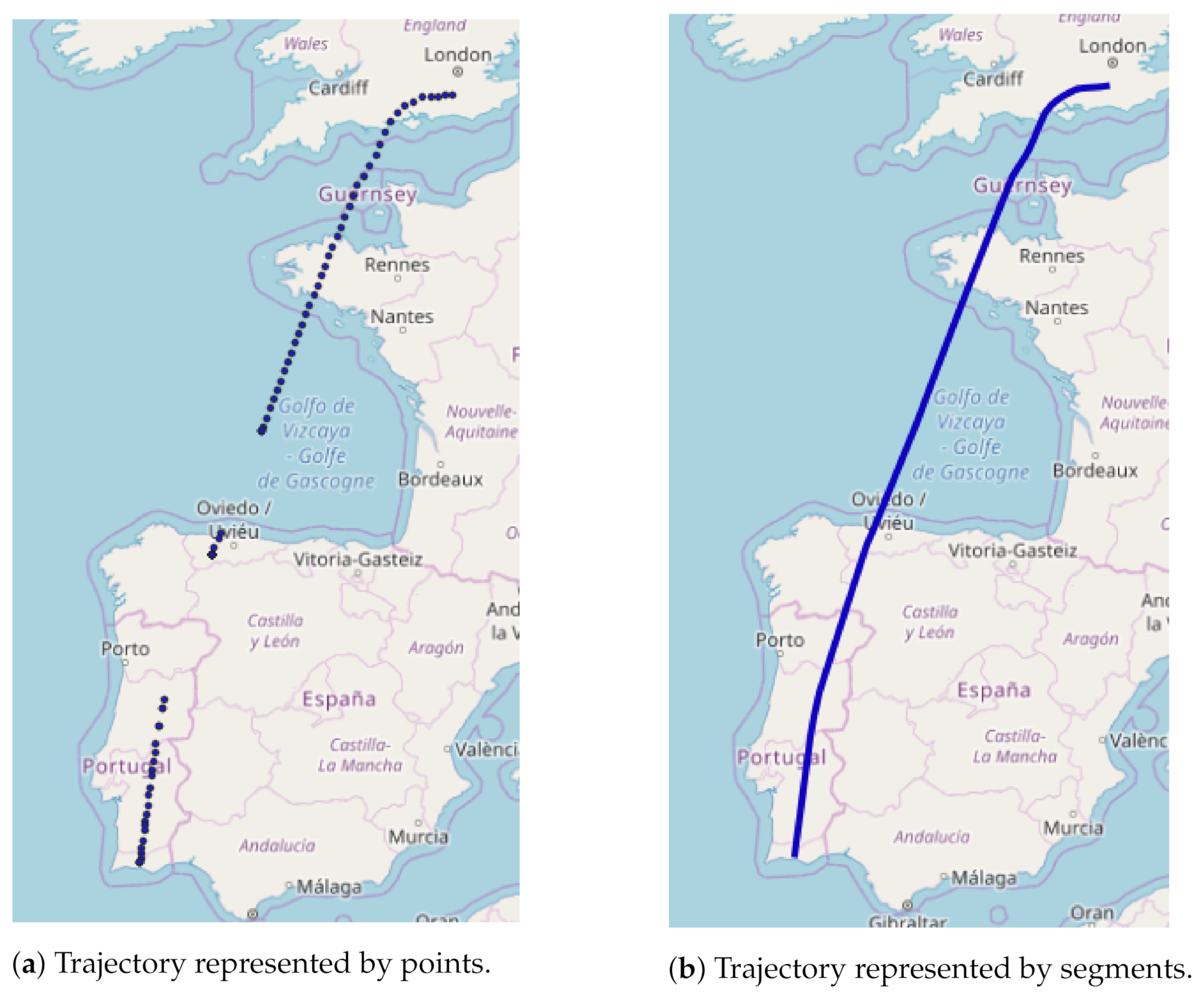
Next, we use the position messages to construct the trajectories using the Well-Known-Text (WKT) format, creating segments in 3D that are then linked into trajectories, each representing a specific flight. We chose to use segments to overcome the problem of missing position data points in the areas of the low sensor coverage, as depicted in Figure 1. Moreover, use of segments makes the trajectory clustering process (described in the following section) easier to implement.
3.2. Applied Techniques
3.2.1. DBSCAN
Different data mining techniques were mentioned in Section 2. Since we cannot estimate the correct number of typical clusters a priori, we cannot use partitional clustering. Hierarchical and density-based approaches are in principle suitable as they do not require to estimate a priori the number of clusters. However, the way the hierarchical clustering works is generally more complex than the density-based one, of which DBSCAN is the most common and simple, and has already been widely used for clustering aircraft trajectories (see, e.g., Annoni and Forster [19], Gariel et al. [8], Olive and Basora [30], Olive and Basora [31]). In fact, DBSCAN does not require to be initialised with the number of clusters to create, as it autonomously finds the number of clusters suitable for the problem.
DBSCAN clusters elements that are closely packed together, that is to say, elements in a -neighbourhood and surrounded by a minimum number of neighbours. It requires two parameters: the maximum radius of the neighbourhood and the minimum number of elements m required for a cluster.
An element q is in the neighbourhood of an element p if , where is the distance between the two points p and q. If the number of neighbours of p is greater or equal to m, then a new cluster is created with p as core element. All the -neighbours of p are elements of . If a core element of a cluster is added to a cluster , these two clusters are merged together. DBSCAN iteratively adds elements to clusters until all elements are assigned.
The parameters choice of DBSCAN was based on air traffic management characteristics. We set maximum radius of the neighbourhood (which corresponds to 30 km; an airway has a width of 10 NM, which equals 18.52 km, to which we added a buffer) and a minimum number of elements (since we do not consider a lone trajectory to be a cluster) as parameters of the DBSCAN algorithm.
Here, an element for DBSCAN is a flight trajectory. As explained above in Section 3.1.2, a trajectory is a geometric representation of a set of connected position messages of that flight (latitude, longitude and altitude). The distance between two elements is represented by the undirected Hausdorff distance.
The Hausdorff distance is the maximum distance of a trajectory to the nearest measurement in the other trajectory. In other words, given a distance d and a two trajectories P and Q, the Hausdorff distance h can be calculated as:
where p and q are the single coordinates belonging to the respective trajectories. This distance is not a metric since it is not symmetric; therefore, we used the undirected version, which can be calculated as the maximum of the two directed distances changing the order of the operands:
One of the main advantages of using this distance is that it does not require the two trajectories to be composed of the same number of position messages. To efficiently calculate the Hausdorff distance, we applied the method proposed by [32]. Internally, in the Hausdorff distance between two trajectories, the distance between two measurements is approximated with the Euclidean distance. Therefore, 1 degree of difference in latitude is around 110 km and we also approximate the longitude difference with 110 km due to the fact that the flights we consider in this work are all located in Europe.
As we are looking into 3D flight trajectories, we need to take into account latitude, longitude and altitude, as altitude plays an important role in proper clustering. For example, an aircraft type A and aircraft type B can fly exactly the same 2D trajectory (latitude, longitude), but the type A cannot go over an altitude X, while type B can. Thus, when taking 3D environment into account, the trajectories of these two aircraft types should belong to different clusters. This requires a slight modification of the DBSCAN algorithm as the horizontal distance between the elements is measured in kilometres, while the difference in altitude is measured in meters (e.g., the distance between two flight levels is 1000 ft, which is about 300 m). Therefore, to properly take into account the altitude value, we scaled it by a factor in order to create clusters that make sense altitude-wise as well. We set .
3.2.2. Pearson’s Test
After the clustering of trajectories between different OD pairs, we employ the Pearson’s test for the further analyses. A Pearson’s test of independence compares the frequency of collected, categorically grouped data (in the contingency table—a matrix that shows the frequency distribution of multivariate variables), with the frequencies one would expect to obtain in the same contingency table by chance alone (known as the expected frequencies). The lower the p-value, the greater the dependence, whereas, with the high p-value, the null hypothesis of independence cannot be rejected.
The test of independence is applied to discern if the obtained clustering indicates relations between trajectories, airlines, aircraft cost models and flight cost profiles. Note that to be able to apply the Pearson’s test, each variable under analysis has to have at least two values.
4. Initial Analyses
This section reports the results from the initial data investigation, used to further fine-tune the data-mining analyses. First, the initial data inspection is presented, describing the available data and reasons for exclusion or inclusion in the main analysis. The second part describes clusters obtained through application of DBSCAN with parameters defined in Section 3.2.1.
4.1. Initial Data Inspection
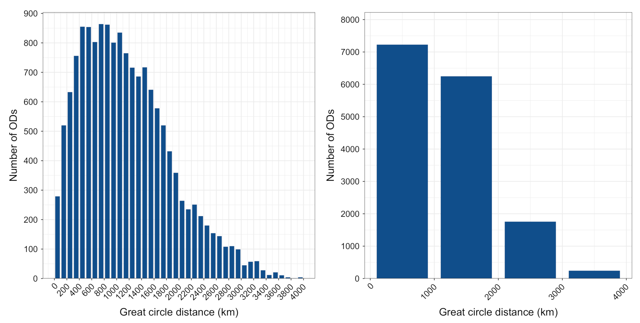
The dataset prepared by the algorithm described in Section 3.1 contains 1,443,062 flights, flown between 15,184 OD pairs. The average great circle distance between these OD pairs is 1167 km. Figure 2 shows the histogram of the number of OD pairs across the distances. The left graph groups the OD pairs in bins of 100 km distances, while the right graph groups in bins of 1000 km. We notice that as many as 279 OD pairs only involve “positioning” flights. Positioning refers to moving an aircraft, without passengers, from one airport to another at the end (or beginning) of the day, to be ready for the following scheduled flights. They are characterised by a very short distance, always less than 100 km. The shortest great circle distance is of 7.6 km between the two Bucharest airports. Another interesting example includes Paris Charles de Gaulle and Paris Orly (34 km). Between Charles de Gaulle and Orly, there were 119 flights, operated by eight airlines, while, in the opposite direction, there were 79 flights, operated by seven airlines. As we are interested in the scheduled flights, all the positioning flights are excluded from the analysis.
Figure 2 (right panel) shows that a good portion (about 45 %) of OD pairs has a great circle distance that is less than 1000 km. The majority of these OD pairs ( 68 %) had only one airline that operated the flights in the season, and 250 of these ODs had more than 1000 flights, or six flights a day, on average. Such frequency indicates hub-feeder flights.
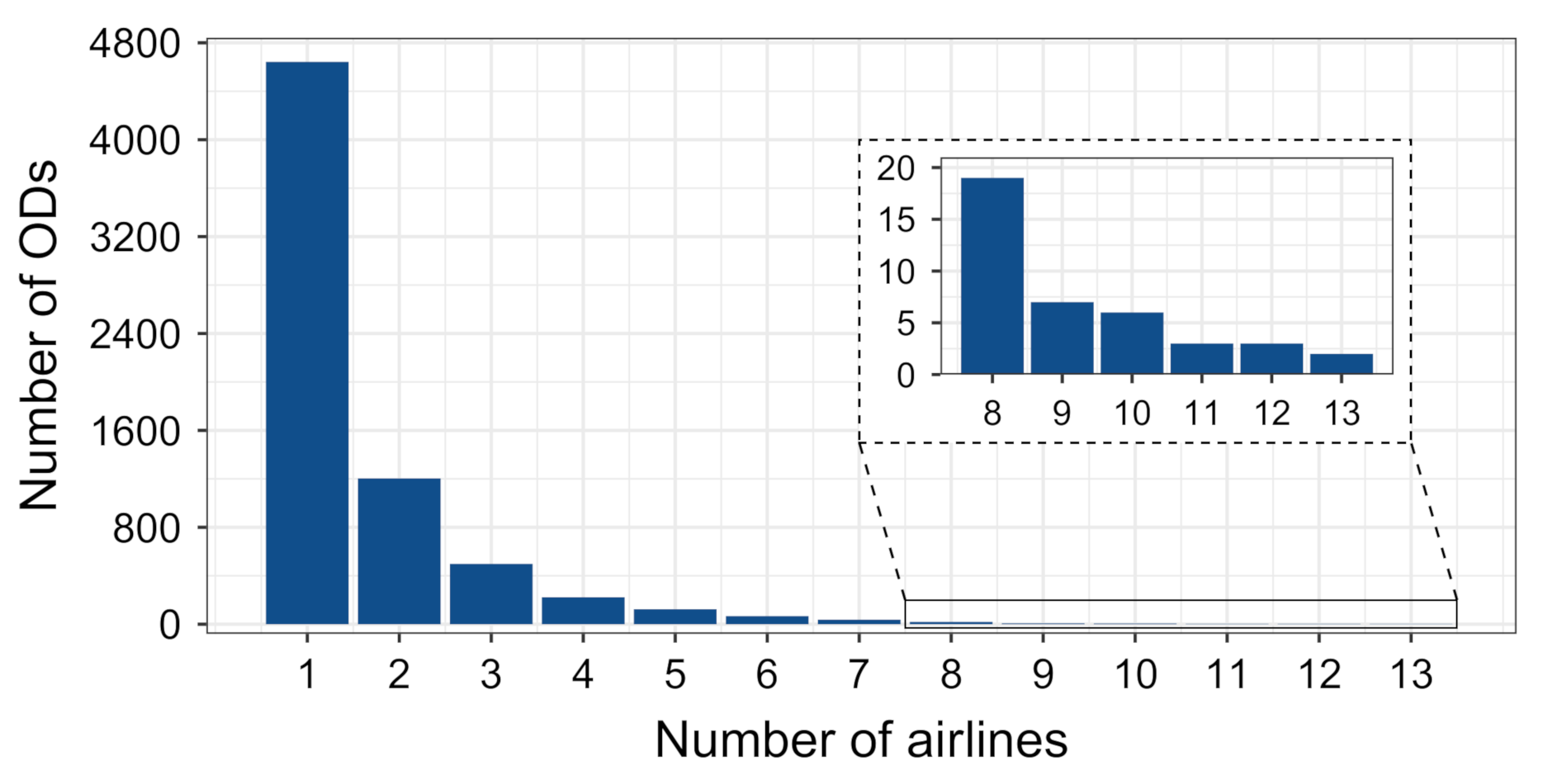
Furthermore, Figure 3 shows the distribution of number of airlines serving ODs with great-circle distance (GCD) that is less than 1000 km. As can be seen, most are served by one airline, but there are those with more than five, up to 13 airlines. On closer inspection of related data, in many cases, there are two to four airlines with a significant number of flights, while others operate just a handful of flights. For example, between Munich and Frankfurt, there were 2964 flights, belonging to 13 airlines. Three airlines operated 99 % of the flights, while other 10 airlines accounted for one, two, three or four flights in the six-month period.
The analysis of the number of flights by airlines within an OD pair revealed that some airlines operated only a handful of flights during the 2019 summer season, which is composed of 30 weeks. As already mentioned, we are interested in the scheduled flights. Usually, scheduled services have at least one flight a week (we are aware that some services start later in the season, but we do not have access to schedules to confirm or disprove on a case by case basis). Thus, we decided that if an OD pair, or an airline that operates flights for an OD pair, has less than 30 flights, they should be excluded from the further analyses. Another reason is that, for the further analysis, we need a statistically relevant number of flights. The ODs with less than 30 flights in the summer season mostly indicate weekly flights to summer destinations. Most of these destinations involve secondary airports. For example, the airport with the most originating flights to be removed due to this constraint is Copenhagen, as it had 15 such summer destinations.
4.2. Clustering Characteristics
This section describes the initial results of the DBSCAN clustering, as described in Section 3.2.1. As stated in the Introduction, we want to verify if the distributions of flight trajectories into clusters depends on the following variables: airline, aircraft type and flight cost profile. To be able to perform these analyses, we first study the results of the clustering, which is then used to tailor the subsequent analyses.
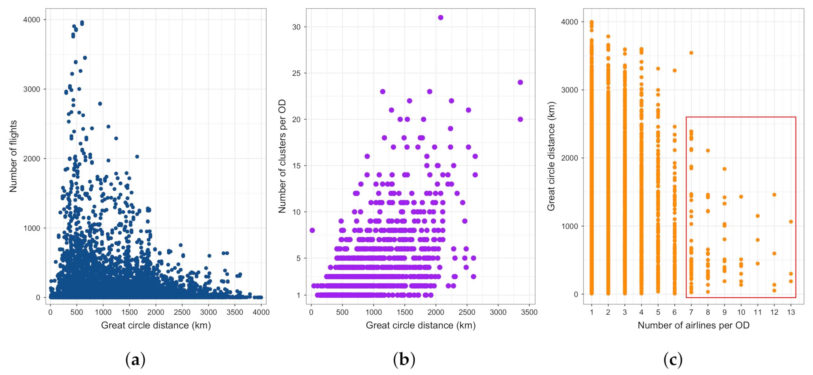
Figure 4 depicts the relation between the GCD between the ODs and three other factors: number of flights, number of clusters between ODs and number of airlines serving the ODs. ODs with the highest number of flights (≥2500) have GCD between about 400 and 1000 km. As discussed above, this is probably the effect of feeder flights into the hubs. Next, as the distance between the origin and destination airports increases, so does the number of trajectory clusters. The maximum number of clusters can be found for ODs with the distance of about 2500 km. It is not a linear relationship as some distant ODs also have a low number of clusters. For example, between Madrid and Stockholm Arlanda airports, we have three trajectory clusters, even though the GCD is slightly greater than 2500 km. The OD with most clusters is Istanbul Sabiha and Düsseldorf, having 31 clusters. Furthermore, Figure 4c shows the number of airlines depending on the GCD between the ODs. The majority of ODs, regardless of GCD, is served by one to four airlines. However, we can see that, for some ODs, there can be more than seven airlines, going up to 13. These are located within the red rectangle as most of the counted airlines operated just a handful of flights. As such, many of the counted airlines will be discarded from the further analyses, as explained in the previous section.
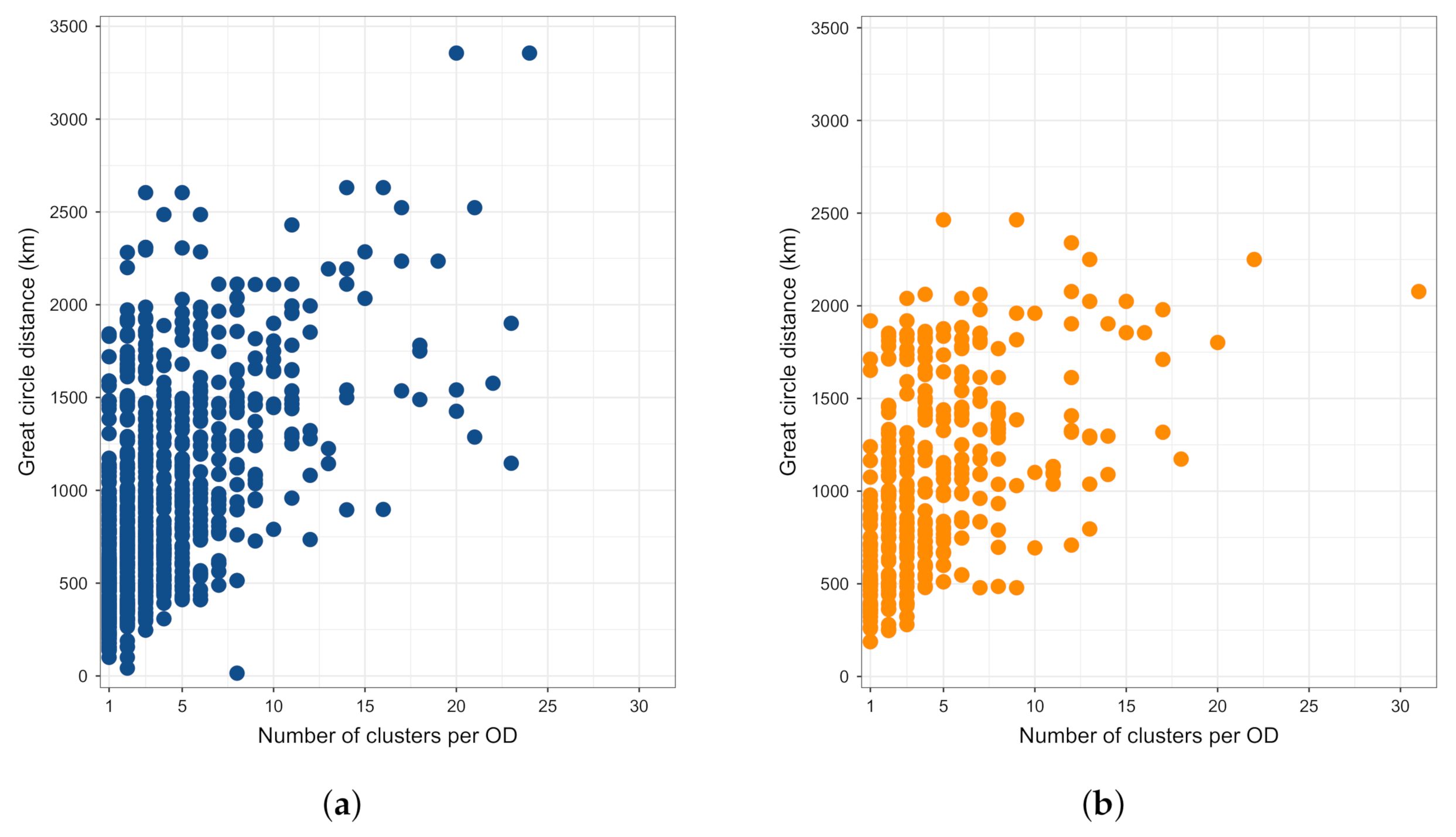
Turning to the next variable of interest, the aircraft type, Figure 5 explores the relationship between the aircraft type, GCD and number of clusters between the ODs (for each OD, we have its GCD, number of aircraft types and number of resulting trajectory clusters between ODs). As can be seen in Figure 5a, two aircraft types are the most frequent case between the ODs, especially in the most travelled GCD range (i.e., 500–1000 km). Furthermore, about 10 % of ODs are served by only one aircraft type. Figure 5b shows that the majority of ODs being served by two aircraft types has less than five clusters between the OD. In addition, the vast majority of the ODs has up to 10 clusters. There is a relatively small number of ODs with more than 10, going up to 31 clusters.
A cost profile of a flight depends on the airline’s business model (e.g., legacy carrier) and the type of a flight (e.g., point-to-point or hub feeder), a type depending on the position the origin and destination play in the route network of that particular airline. As explained in Section 3.1, we assigned three profiles—low, base and high. Figure 6 shows relations between the number of cost types, GCD and the number of clusters per OD. The graph shows that ODs with one or two cost profiles are similarly distributed across the GCD and number of clusters.
To be able to apply the Pearson’s test, each variable has to have at least two values. This initial data inspection reveals that, in order to perform further analyses for each of the variables we are interested in, i.e., number of airlines, number of aircraft types and number of cost profiles, we would need to create specific data subsets. For the analysis of the number of airlines, we need to remove all the ODs that are served by only one airline. The same applies for the aircraft types and cost profiles.
5. Results of Variables’ Relations Analyses
This section describes the results of the analyses of the relation trajectory clusters have with the three variables of interest: airlines, aircraft type and cost profile.
5.1. Relation between Clusters and Airlines
The first relation we want to analyze is the one between trajectory clusters and airlines. To do that, we removed from the analysis:
- the OD pairs served by only one airline;
- the OD pairs with less than 30 flights;
- and, for each OD, flights by an airline that had less than 30 flights in the season between that OD.
After the removals, we have 860 OD pairs and 529,011 flights. We performed the Pearson’s test comparing the distribution of trajectories among clusters and airlines, having created contingency tables for each OD pair retained in this analysis. Results show that, at a confidence level , in about 49 % of OD pairs, the choice of the trajectory is dependent on the airline performing the flight. Four graphs in Figure 7 depict the relations between the number of airlines and the following variables: number of clusters, number of flights, and the GCD between OD pairs. The “Dependent” category describes the data for OD pairs where the dependence between the airlines and the clusters is found, while the opposite is true for the “Not dependent” category.
As can be seen in Figure 7a, even when the ODs are served by multiple airlines, but there is a small number of trajectory clusters between them, the choice of a particular cluster does not depend on an airline performing a flight. In all the Not dependent cases, the average number of clusters is less than five, even though there are some values that fall outside the upper quartile value (most of them for ODs with two airlines). From Figure 7b, we can note that, with the increase of the number of airlines up to four, the average number of flights between the ODs remains almost the same, whereas the number of flights between the ODs with five airlines is higher. Another interesting characteristic can be noted in Figure 7c, where the average GCD between ODs where we find dependence between the airline and the trajectory cluster flown is on average higher than between those where such relations do not exist. Figure 7d shows distribution of Dependent and Not dependent ODs across number of airlines and GCD.
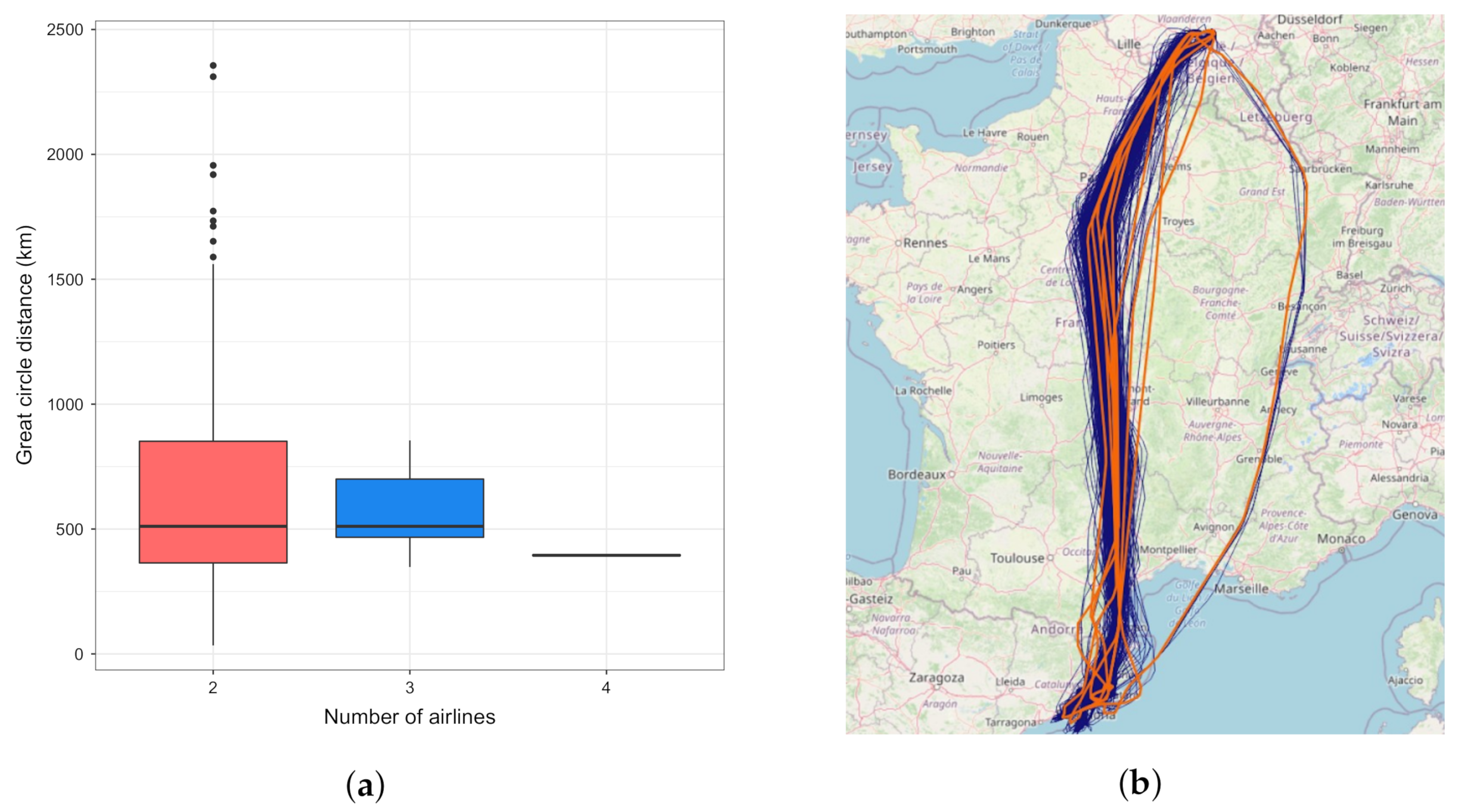
Among the Not dependent ODs, there are 149 that have only one trajectory cluster; thus, it could be said that all airlines plan the same trajectory between those ODs. As can be seen in Figure 8a, the average GCD for those OD pairs is less than 1000 km. This, and the fact that other OD pairs with average GCD around 1000 km mainly do not demonstrate the dependence between the airline and trajectory cluster (see Figure 7c) lead us to the conclusion that for the “short” flights, it is usual, by all airlines, to plan along the same trajectory cluster. The closer inspection of other ODs where we do not find the relation between the trajectory clusters and airlines, shows that, in those cases, there is usually one dominant cluster that all airlines use, while other clusters have only several flights, equally distributed among different airlines. Figure 8b depicts all the trajectories (in blue) between Brussels and Barcelona airports, and the 10 cluster centroids (orange lines). Three airlines serve the OD pair, each flying about a third of total 1517 flights. About 98 % of all flights are performed along the dominant cluster, while there are only token flights in other clusters.
Let us turn to the OD pairs where we find the dependence between the airline and chosen cluster. Table 1 shows the distribution of airlines’ flights across the four clusters for Rome Fiumicino–Warsaw Chopin OD pair, while the data for Milan Malpensa–Bari airports can be found in Table 2. Between Rome Fiumicino–Warsaw, Airline 2 tends to use cluster 0, while Airline 1 uses almost exclusively cluster 3. Moreover, Airline 2 has a few flights belonging to clusters 1 and 2. It is likely that the different trajectory is due to some issue along the usual route. The issue could be related to the bad weather along the portion of the route, or lack of capacity of air transport network (e.g., lack of air traffic controllers, union action).
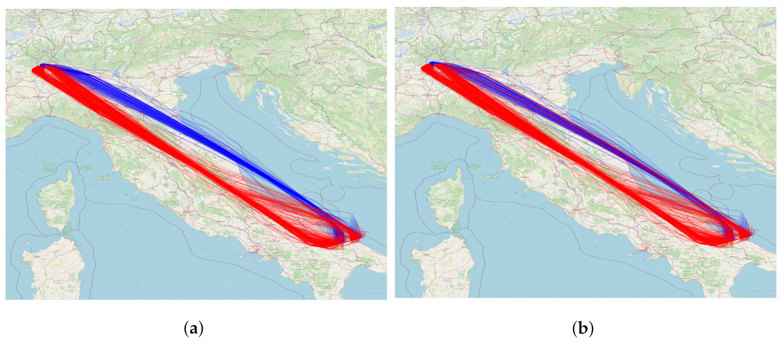
In Table 2, we can see that two airlines fly along two different clusters. Cluster 0 is favoured by Airline 2, while cluster 0 is favoured by Airline 1. There are two Airline 2 flights in cluster 1, on different days, and a few Airline 1 flights in cluster 0. As above, this is probably due to some issue that was specific to those two days. Figure 9 depicts all the trajectories between Milan Malpensa and Bari.
To sum up, for the OD pairs where we do obtain the dependence between the cluster and airline, it is possible to identify different trajectory usage by airlines. However, note that cluster usage should be inspected, as some clusters have very low usage and are indicative of specific issues on the days (e.g., cluster 2 in Table 1), not the regular usage across the season.
5.2. Relation between Clusters and Aircraft Types
The next relation we want to analyse is the one between trajectory clusters and aircraft types. To do that, we removed from the analysis:
- the OD pairs served by only one aircraft type;
- the OD pairs with less than 30 flights;
- and, for each OD, flights by an aircraft type that had less than 30 flights in the season between that OD,
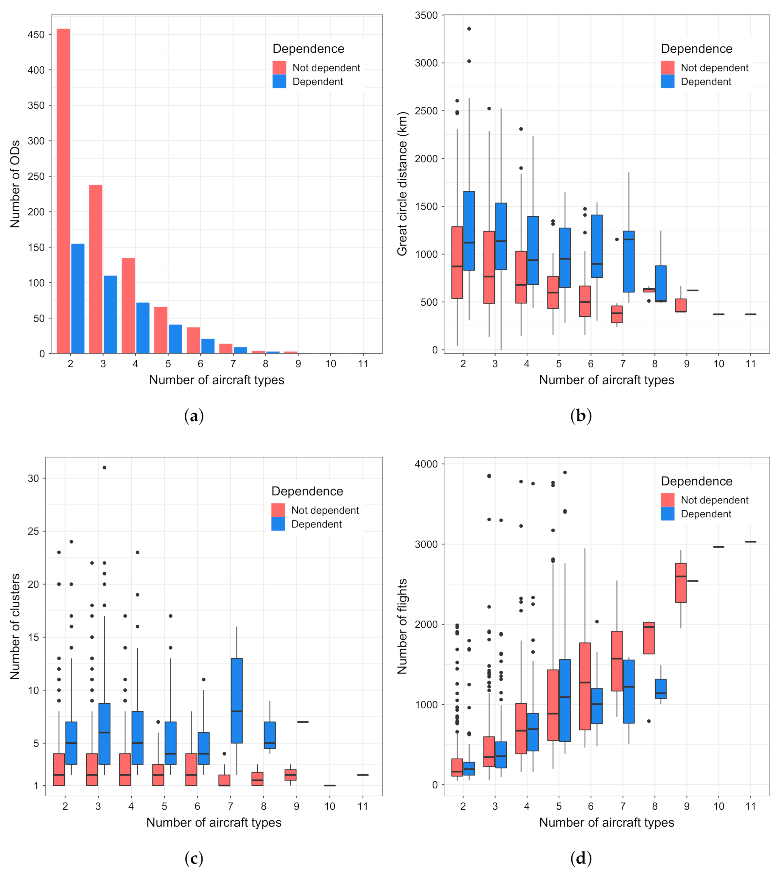
which leaves us with the 751,281 flights serving 1369 OD pairs. During the season under analysis, 91 distinct aircraft types were used. As in the previous case, the Pearson’s test was performed in the analysis. The test shows dependence (with , p-value ≤ 0.05) between the trajectory cluster and the aircraft type for 30 % of the ODs. Figure 10 depicts the results of the analysis.
Figure 10a shows that the number of aircraft types used between ODs ranges from two to at the most eleven. The great majority of OD pairs is served by two aircraft types, then three and four types. Less than 100 OD pairs are served by more than five aircraft types. Figure 10b shows that, in all aircraft type categories, we can find the dependence between the trajectory clusters and number of aircraft types for ODs that are further apart. Overall, the average GCD is lower than 1000 km in all the Not dependent cases. Here, we can observe an interesting case of ODs served by nine aircraft types that show almost no dependence. One such OD is Helsinki–Stockholm Arlanda, being less than 400 km apart. In this case, 99 % of flights use the same, predominant trajectory, and the remaining flights are distributed across other three trajectory clusters. Figure 10c shows that, between the ODs, we find dependence between the trajectory clusters and aircraft types having more clusters between them than in cases with no dependence found. Furthermore, Figure 10d shows that we may find more aircraft types serving ODs with a higher number of flights between them.
5.3. Relation between Clusters and the Cost Profile
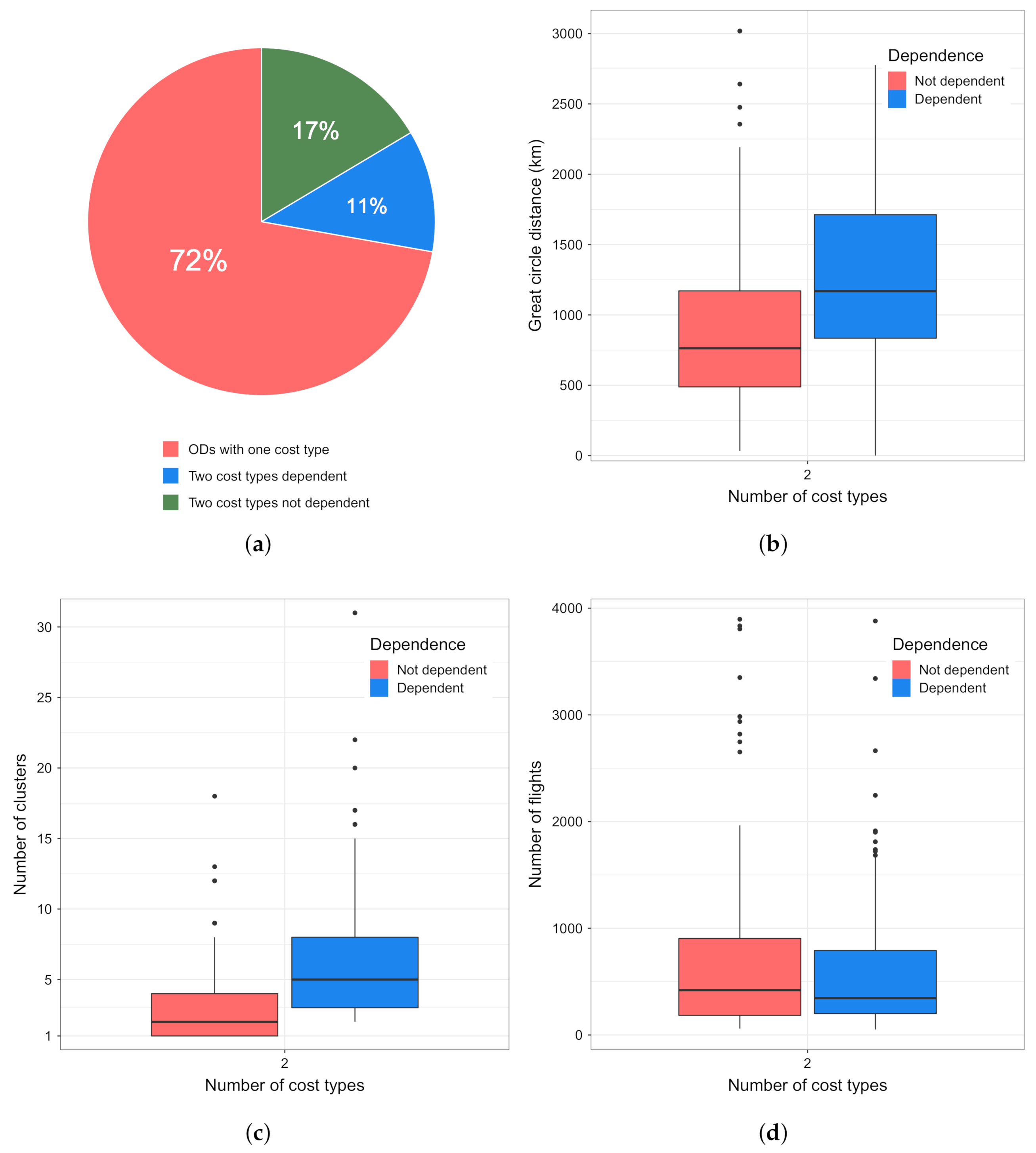
Finally, we want to analyze if a relation exists between the trajectory chosen and the cost profile of the flight. It is worth repeating that, with a cost profile, we are assigning low, base, or high operational costs to a flight. The level of costs depends on the airline’s business model (e.g., legacy carrier) and the type of a flight (e.g., point-to-point or hub feeder). Figure 11a shows that, between the majority OD pairs ( 72 %), only one cost type can be assigned, which is to be expected. As in the previous two cases, we remove:
- the OD pairs with one cost type;
- the OD pairs with less than 30 flights.
The remaining 428 OD pairs are served by 265,575 flights. The flights between these OD pairs can be assigned to two cost profiles.
About 45 % of OD pairs in the analysis shows that the dependence between the cost type and the cluster flown exists (see Figure 11a). The closer OD pairs are less likely to show dependence, as can be seen in Figure 11b. Dependent OD pairs on average have the GCD of about 1260 km, while those not dependent are on average 910 km closer. Moreover, also in this analysis, we can see that a low number of trajectory clusters between OD pairs does not produce dependence (see Figure 11c). ODs that on average have a higher number of clusters show that a relation between the cost type and cluster flown exists. In Figure 11d, we can see that the not dependent and dependent OD pairs on average have a similar number of flights.
The results of this analysis are very similar to those of the relation between the clusters and airlines, due to the manner of assigning the cost profile to flights (see Section 3.1), which sees all the flights of an airline serving an OD having the same cost profile. Table 3 shows the contingency table for Madrid–London Gatwick OD pair, which has high dependence in both analyses (p-value < 0.001 for cost type and airline). The legacy airlines 2, 3 and 4 (high cost profile) mostly use cluster 0, while the low cost airline 1 tends to use both clusters, with a preference for the cluster 1. The data sets used in the airline and then cost type analyses are different. However, if we compare the OD pairs that show relation between the trajectory cluster and airline, and trajectory cluster and cost profile, we see that almost all ( 96 %) OD pairs that show dependence for the cost type show the same behaviour in the airline analyses. This suggests that it makes more sense to use the airline variable to check for relations between trajectory clusters flown. In the airline analysis, we had 860 OD pairs, and 428 in this one, pointing that 432 OD pairs were served by airlines having the same cost profile.
Another interesting feature regarding the Madrid–London Gatwick OD pair is that it has high dependence also in the aircraft type analysis (p-value < 0.001). The motivation behind this fact can be inferred by looking at the contingency table of airline vs. aircraft type for this OD (see Table 4), which shows a high dependence between these two variables. There is only one airline that employs two aircraft types for that OD, while the other three employ only one aircraft type. A similar behaviour can be found in several other OD pairs that have high dependence in all the variables of interest (airline, aircraft type, cost profile).
6. Conclusions
Relying on an extensive dataset, this work quantifies to what extent airline usual trajectories depend on the airline itself, the aircraft type that operated the flight, and associated cost profiles.
The analysis reveals interesting characteristics of the European air traffic, which can be used as input in various air traffic modelling activities. One of the results shows that about 58 % of flights is between OD pairs that are closer than 1000 km, and are mostly served by one airline (see Figure 3). What is even more interesting is that, at these distances, only one trajectory cluster, i.e., one planned trajectory is being used. Even in cases where more than one cluster can be identified, one is predominant and the others have token flights. In the current setting, where the airlines choose aircraft types and trajectories in order to minimise the operational costs, this is to be expected. The inclusion of environmental indicators that are not limited to the CO2 might bring a change to this type of choice.
ODs with higher GCD between them are more likely to exhibit the relation between the trajectory cluster flown and the airline, showing that, at these longer distances, we can find that different airlines can opt for different choices. Furthermore, for OD pairs where we do obtain the dependence between the cluster and airline, the cluster usage should be inspected, as some clusters have very low usage and are indicative of specific issues on the days (e.g., cluster 2 in Table 1), not the regular usage across the season.
Similarly, the relation between the aircraft type and trajectory cluster can be found for ODs that are further apart, and that have a higher number of trajectory clusters. We could see that the majority of OD pairs are served by one type of cost profile flights, which is to be expected. For example, ODs that are less than 1000 km apart, and served with only one airline, can be assigned only one cost profile, as flight costs depend on the aircraft type used and the airline type. For OD pairs where we could perform this analysis, i.e., where at least two cost types operated between the OD pairs, almost all ( 96 %) OD pairs that show dependence for the cost type show the same behaviour in the airline analyses. This shows that it makes more sense to use the airline variable to check for relations between trajectory clusters flown.
We demonstrated that the historical analysis of the flown trajectories can indicate the OD pairs where the choice of trajectory clusters depends on the airline operating the flights, of aircraft types used for different distances, at the European network level. These results could be further extended by exploring the impact of more than variables, and adding other characteristics like time-of-day. Differential use of trajectory clusters between different airlines serving the same OD pairs can be used for modelling future scenarios (e.g., traffic network in 2030) in air traffic management, enabling more accurate characterisation of flights, even between ODs that are currently not within airlines’ route networks. Another interesting example of the usage of our results could be in the investigation of air and rail travel competition or collaboration. As we mentioned already, around half the flights in European zone are short-haul (i.e., less than 1500 km) and thus in some cases candidates for substitution by rail. Knowing that on such OD pairs only one trajectory cluster is used, it would be easy to assess the impact on demand reduction in certain portions of airspace in case the air service is replaced by the rail one.
Furthermore, the extension of the analysed period to include the winter season would give a more complete picture of the airline choices on the chosen trajectories.
We finally recall that this work is entirely based on data open for research purposes. As a drawback, the dataset needs accurate cleaning. However, the availability of a large dataset of actually flown trajectories made this analysis possible, as more complete data from proprietary sources would be prohibitively expensive for research purposes.
Author Contributions
Conceptualization, T.B. and L.C.; methodology, T.B. and A.D.L.; software, F.V.; validation, T.B. and L.C.; formal analysis, A.D.L. and F.V.; investigation, T.B., A.D.L. and F.V.; resources, T.B. and L.C.; data curation, F.V.; writing—original draft preparation, T.B. and F.V.; writing—review and editing, T.B. and L.C.; visualization, F.V.; supervision, T.B. and L.C.; project administration, T.B. and L.C.; funding acquisition, not applicable. All authors have read and agreed to the published version of the manuscript.
Funding
This research received no external funding.
Institutional Review Board Statement
Not applicable.
Informed Consent Statement
Not applicable.
Data Availability Statement
All raw data have been sourced from https://opensky-network.org on 20 December 2021 and are freely available for research purposes.
Conflicts of Interest
The authors declare no conflict of interest.
Abbreviations
The following abbreviations are used in this manuscript:
| ACI | Airports Council International |
| ADS-B | Automatic Dependent Surveillance-Broadcast |
| DBSCAN | Density-Based Spatial Clustering of Applications with Noise |
| ECAC | European Civil Aviation Conference |
| GCD | Great-Circle Distance |
| MTOW | Maximum Take-off Weight |
| OD | Origin-Destination |
| TMA | Terminal Manoeuvring Area |
References
- Bourgois, M.; Sfyroeras, M. Open data for air transport research: Dream or reality? In Proceedings of the International Symposium on Open Collaboration, Berlin, Germany, 27–29 August 2014; p. 17. [Google Scholar]
- Spinielli, E.; Koelle, R.; Barker, K.; Korbey, N. Open Flight Trajectories for Reproducible ANS Performance Review. In Proceedings of the SIDs 2018, 8th SESAR Innovation Days, Salzburg, Austria, 4–6 December 2018. [Google Scholar]
- Schafer, M.; Strohmeier, M.; Smith, M.; Fuchs, M.; Pinheiro, R.; Lenders, V.; Martinovic, I. OpenSky report 2016: Facts and figures on SSR mode S and ADS-B usage. In Proceedings of the 2016 IEEE/AIAA 35th Digital Avionics Systems Conference (DASC), Sacramento, CA, USA, 25–29 September 2016; pp. 1–9. [Google Scholar] [CrossRef]
- MacQueen, J. Some methods for classification and analysis of multivariate observations. Berkeley Symp. Math. Stat. Probab. 1967, 1, 281–297. [Google Scholar]
- Murtagh, F.; Contreras, P. Algorithms for hierarchical clustering: An overview. Wiley Interdiscip. Rev. Data Min. Knowl. Discov. 2012, 2, 86–97. [Google Scholar] [CrossRef]
- Ankerst, M.; Breunig, M.M.; Kriegel, H.P.; Sander, J. OPTICS: Ordering points to identify the clustering structure. ACM Sigmod Rec. 1999, 28, 49–60. [Google Scholar] [CrossRef]
- Ester, M.; Kriegel, H.P.; Sander, J.; Xu, X. A density-based algorithm for discovering clusters in large spatial databases with noise. Kdd 1996, 96, 226–231. [Google Scholar]
- Gariel, M.; Srivastava, A.N.; Feron, E. Trajectory clustering and an application to airspace monitoring. IEEE Trans. Intell. Transp. Syst. 2011, 12, 1511–1524. [Google Scholar] [CrossRef] [Green Version]
- Basora, L.; Morio, J.; Mailhot, C. A Trajectory Clustering Framework to Analyse Air Traffic Flows. In Proceedings of the SIDs 2017, 7th SESAR Innovation Days, Belgrade, Serbia, 28–30 November 2017. [Google Scholar]
- Nicol, F.; Puechmorel, S. Unsupervised aircraft trajectories clustering: A minimum entropy approach. In Proceedings of the ALLDATA 2016, Lisbonne, Portugal, 21–25 February 2016; pp. 35–41. [Google Scholar]
- Puechmorel, S.; Nicol, F. Entropy minimizing curves with application to flight path design and clustering. Entropy 2016, 18, 337. [Google Scholar] [CrossRef] [Green Version]
- Olive, X.; Basora, L. Identifying Anomalies in past en-route Trajectories with Clustering and Anomaly Detection Methods. In Proceedings of the Thirteenth USA/Europe Air Traffic Management Research and Development Seminar (ATM2019), Vienna, Austria, 17–21 June 2019. [Google Scholar]
- Olive, X.; Basora, L.; Viry, B.; Alligier, R. Deep Trajectory Clustering with Autoencoders. In Proceedings of the International Conference for Research in Air Transportation (ICRAT 2020), Virtual Event, 15 September 2020. [Google Scholar]
- Corrado, S.J.; Puranik, T.G.; Pinon, O.J.; Mavris, D.N. Trajectory Clustering within the Terminal Airspace Utilizing a Weighted Distance Function. Proceedings 2020, 59, 7. [Google Scholar] [CrossRef]
- Poppe, M.; Buxbaum, J. Clustering Climb Profiles for Vertical Trajectory Analysis. In Proceedings of the SIDs 2020, 10th SESAR Innovation Days, Virtual Event, 7–10 December 2020. [Google Scholar]
- Chen, G.; Rosenow, J.; Schultz, M.; Okhrin, O. Using Open Source Data for Landing Time Prediction with Machine Learning Methods. Proceedings 2020, 59, 5. [Google Scholar] [CrossRef]
- Jesse, C.; Liu, H.; Smart, E.; Brown, D. Analysing flight data using clustering methods. In Proceedings of the International Conference on Knowledge-Based and Intelligent Information and Engineering Systems, Zagreb, Croatia, 3–5 September 2018; Springer: Berlin/Heidelberg, Germany, 2008; pp. 733–740. [Google Scholar]
- Ayhan, S.; Samet, H. Time series clustering of weather observations in predicting climb phase of aircraft trajectories. In Proceedings of the 9th ACM SIGSPATIAL International Workshop on Computational Transportation Science, Burlingame, CA, USA, 31 October–3 November 2016; pp. 25–30. [Google Scholar]
- Annoni, R.; Forster, C.H. Analysis of aircraft trajectories using fourier descriptors and kernel density estimation. In Proceedings of the 2012 15th International IEEE Conference on Intelligent Transportation Systems, Anchorage, AK, USA, 16–19 September 2012; pp. 1441–1446. [Google Scholar]
- Mcfadyen, A.; O’Flynn, M.; Martin, T.; Campbell, D. Aircraft trajectory clustering techniques using circular statistics. In Proceedings of the 2016 IEEE Aerospace Conference, Big Sky, MT, USA, 5–12 March 2016; pp. 1–10. [Google Scholar]
- Marcos, R.; Ros, O.G.C.; Herranz, R. Combining Visual Analytics and Machine Learning for Route Choice Prediction. In Proceedings of the SIDs 2017, 7th SESAR Innovation Days, Belgrade, Serbia, 28–30 November 2017. [Google Scholar]
- Evans, A.D.; Lee, P.U. Using machine-learning to dynamically generate operationally acceptable strategic reroute options. In Proceedings of the Thirteenth USA/Europe Air Traffic Management Research and Development Seminar (ATM2019), Vienna, Austria, 17–21 June 2019. [Google Scholar]
- Rehm, F. Clustering of flight tracks. In Proceedings of the AIAA Infotech@ Aerospace 2010, Atlanta, GA, USA, 20–22 April 2010; American Institute of Aeronautics and Astronautics: Reston, VA, USA, 2010; p. 3412. [Google Scholar]
- Atev, S.; Miller, G.; Papanikolopoulos, N.P. Clustering of vehicle trajectories. IEEE Trans. Intell. Transp. Syst. 2010, 11, 647–657. [Google Scholar] [CrossRef]
- Chen, J.; Wang, R.; Liu, L.; Song, J. Clustering of trajectories based on Hausdorff distance. In Proceedings of the 2011 International Conference on Electronics, Communications and Control (ICECC), Ningbo, China, 9–11 September 2011; pp. 1940–1944. [Google Scholar]
- Cook, A.J.; Tanner, G. European Airline Delay Cost Reference Values; Technical report; EUROCONTROL Performance Review Unit: Brussels, Belgium, 2015. [Google Scholar]
- Bolić, T.; Castelli, L.; Corolli, L.; Rigonat, D. Reducing ATFM delays through strategic flight planning. Transp. Res. Part E Logist. Transp. Rev. 2017, 98, 42–59. [Google Scholar] [CrossRef] [Green Version]
- Bolić, T.; Castelli, L.; Rigonat, D. Peak-load pricing for the European Air Traffic Management system using modulation of en-route charges. Eur. J. Transp. Infrastruct. Res. 2017, 17. [Google Scholar] [CrossRef]
- ACI Europe. Top 30 European Airports 2017; Technical Report; Airports Council International: Montréal, QC, Canada, 2017. [Google Scholar]
- Olive, X.; Basora, L. A python toolbox for processing air traffic data: A use case with trajectory clustering. In Proceedings of the 7th OpenSky Workshop 2019, Zurich, Switzerland, 21–22 November 2019. [Google Scholar]
- Olive, X.; Basora, L. Detection and identification of significant events in historical aircraft trajectory data. Transp. Res. Part C Emerg. Technol. 2020, 119, 102737. [Google Scholar] [CrossRef]
- Taha, A.A.; Hanbury, A. An efficient algorithm for calculating the exact Hausdorff distance. IEEE Trans. Pattern Anal. Mach. Intell. 2015, 37, 2153–2163. [Google Scholar] [CrossRef] [PubMed]
Figure 1.
Trajectory plotted using points (a) or segments (b), shown in 2D.

Figure 2.
Distribution of the number of OD pairs across a great circle distance between ODs.

Figure 3.
Number of airlines serving ODs with GCD lower than 1000 km.

Figure 4.
Relation between the GCD between ODs and number of flights, number of clusters and number of airlines. (a) GCD vs. number of flights; (b) GCD vs. number of clusters; (c) GCD vs. number of airlines.
Figure 4.
Relation between the GCD between ODs and number of flights, number of clusters and number of airlines. (a) GCD vs. number of flights; (b) GCD vs. number of clusters; (c) GCD vs. number of airlines.

Figure 5.
Relations between the aircraft type, clusters and GCD. (a) Aircraft type vs. GCD length; (b) Aircraft type vs. trajectory cluster.
Figure 5.
Relations between the aircraft type, clusters and GCD. (a) Aircraft type vs. GCD length; (b) Aircraft type vs. trajectory cluster.

Figure 6.
Relations between the flight cost profile, number of clusters and GCD between the ODs. (a) ODs with one cost profile; (b) ODs with two cost profiles.
Figure 6.
Relations between the flight cost profile, number of clusters and GCD between the ODs. (a) ODs with one cost profile; (b) ODs with two cost profiles.

Figure 7.
Depiction of the dependence between the airlines and trajectory clusters, and their distribution across number of flights and GCD between ODs. (a) number of clusters vs. number of airlines; (b) number of flights vs. number of airlines; (c) GCD vs. number of airlines; (d) GCD vs. number of airlines, scatterplot.

Figure 8.
Distribution of GCD for Not dependent, one cluster ODs, and an example of Not dependent, multiple clusters for an OD. (a) Distribution of GCD for OD pairs with one trajectory cluster; (b) trajectory clusters between Brussels and Barcelona.
Figure 8.
Distribution of GCD for Not dependent, one cluster ODs, and an example of Not dependent, multiple clusters for an OD. (a) Distribution of GCD for OD pairs with one trajectory cluster; (b) trajectory clusters between Brussels and Barcelona.

Figure 9.
Trajectories, clusters and distribution of trajectories between airlines serving Milan Malpensa and Bari OD. (a) Cluster 0 (blue) and cluster 1 (red) trajectories; (b) Airline 1 (red) and Airline 2 (blue) trajectories.
Figure 9.
Trajectories, clusters and distribution of trajectories between airlines serving Milan Malpensa and Bari OD. (a) Cluster 0 (blue) and cluster 1 (red) trajectories; (b) Airline 1 (red) and Airline 2 (blue) trajectories.

Figure 10.
Depiction of the dependence between the aircraft types and trajectory clusters, and their distribution across number of flights and GCD between ODs. (a) No. of OD pairs vs. number of aircraft types; (b) GCD vs. number of aircraft types; (c) number of clusters vs. number of aircraft types; (d) number of flights vs. number of aircraft types.

Figure 11.
Depiction of the dependence between the cost types and trajectory clusters, and their distribution across number of flights and GCD between ODs. (a) number of OD pairs with one or two cost types, showing dependence; (b) GCD vs. number of cost types; (c) cost types vs. number of clusters; (d) cost types vs. number of flights.


Table 1.
Contingency table of airline vs. cluster for Rome Fiumicino and Warsaw Chopin airports.
| Cluster | ||||
|---|---|---|---|---|
| Airline | 0 | 1 | 2 | 3 |
| Airline 1 | 0 | 4 | 0 | 169 |
| Airline 2 | 198 | 12 | 3 | 0 |
Table 2.
Contingency table of airline vs. cluster for the Milan Malpensa and Bari airports.
| Cluster | ||
|---|---|---|
| Airline | 0 | 1 |
| Airline 1 | 20 | 346 |
| Airline 2 | 118 | 2 |
Table 3.
Contingency table for Madrid–London Gatwick OD pair, showing the distribution of trajectories across airlines, cost type and clusters.
Table 3.
Contingency table for Madrid–London Gatwick OD pair, showing the distribution of trajectories across airlines, cost type and clusters.
| Cluster | |||
|---|---|---|---|
| Airline | Cost Type | 0 | 1 |
| Airline 1 | Low | 105 | 161 |
| Airline 2 | High | 154 | 1 |
| Airline 3 | High | 176 | 6 |
| Airline 4 | High | 176 | 0 |
Table 4.
Contingency table of airline vs. aircraft type for the Madrid–London Gatwick OD pair.
| Aircraft Type | |||
|---|---|---|---|
| Airline | A | B | C |
| Airline 1 | 187 | 64 | 0 |
| Airline 2 | 0 | 0 | 144 |
| Airline 3 | 0 | 176 | 0 |
| Airline 4 | 0 | 0 | 164 |
Publisher’s Note: MDPI stays neutral with regard to jurisdictional claims in published maps and institutional affiliations. |
© 2022 by the authors. Licensee MDPI, Basel, Switzerland. This article is an open access article distributed under the terms and conditions of the Creative Commons Attribution (CC BY) license (https://creativecommons.org/licenses/by/4.0/).
Share and Cite
MDPI and ACS Style
Bolić, T.; Castelli, L.; De Lorenzo, A.; Vascotto, F. Trajectory Clustering for Air Traffic Categorisation. Aerospace 2022, 9, 227. https://0-doi-org.brum.beds.ac.uk/10.3390/aerospace9050227
AMA Style
Bolić T, Castelli L, De Lorenzo A, Vascotto F. Trajectory Clustering for Air Traffic Categorisation. Aerospace. 2022; 9(5):227. https://0-doi-org.brum.beds.ac.uk/10.3390/aerospace9050227
Chicago/Turabian StyleBolić, Tatjana, Lorenzo Castelli, Andrea De Lorenzo, and Fulvio Vascotto. 2022. "Trajectory Clustering for Air Traffic Categorisation" Aerospace 9, no. 5: 227. https://0-doi-org.brum.beds.ac.uk/10.3390/aerospace9050227
Note that from the first issue of 2016, this journal uses article numbers instead of page numbers. See further details here.