Multi-Layer Fault-Tolerant Robust Filter for Integrated Navigation in Launch Inertial Coordinate System

Abstract

As to an aerospace vehicle, the flight span is large and the flight environment is complex. More than that, the existing navigation algorithms cannot meet the needs to provide accurate navigation parameters for aerospace vehicles, which results in the decline of navigation accuracy. This paper proposes a multi-layer, fault-tolerant robust filtering algorithm of aerospace vehicle in the launch inertial coordinate system to address this problem. Firstly, the launch inertial coordinate system is used as the reference coordinate system for navigation calculation, and the state equation and measurement equation of the navigation system are established in this coordinate system to improve the modeling accuracy of the navigation system. On this basis, a multi-layer, fault-tolerant robust filtering algorithm is designed to estimate and compensate the unknown input in the state equation in real time and adjust the noise variance matrix in the measurement equation adaptively. Simulation results show that the errors about the integrated navigation system output parameters are reduced, through this algorithm, which improves the attitude, velocity and position estimation accuracy of the integrated navigation system. In addition, the algorithm enhances the fault tolerance and robustness of the filtering algorithm.

1. Introduction

In recent years, the trend of air-space integration has been presented in the strategic layout of all military powers around the world. As a new type of aircraft with dual functions of aircraft and spacecraft, the aerospace vehicle (ASV) is gradually occupying an important strategic position in the future battlefield due to its characteristics of cross-airspace, multi-mission, multi-working mode and large-scale high-speed maneuvers [1]. The reusable lifted space vehicles represented by X-37B, IXV, X-33, etc., have attracted more and more attention, promoted the development of low-cost space technology and become a research hotspot in recent years [2,3]. However, their complex motion characteristics throughout the flight process are undoubtedly greatly challengeable to the existing navigation, guidance and control technologies. As an important part of navigation, guidance and control technology, navigation performance directly affects the accuracy of guidance and control loop. Therefore, the advanced navigation technology has become one of the key technologies to be broken through urgently, which is a prerequisite for the safe execution of missions of aerospace vehicles.

The inertial navigation system is completely autonomous and free from electromagnetic signal interference, so it can output complete navigation information. However, due to their own device zero bias and noise, the navigation error of pure inertial navigation systems will increase over time gradually. The satellite navigation system is a high-accuracy geometric positioning and navigation system, with no error accumulating over time [4], but it is difficult to work properly when subject to intentional or unintentional interference [5]. As a high-precision navigation means, celestial navigation systems have a wide range of applications and are completely autonomous, by using natural celestial bodies as navigation beacons. However, due to its complicated solving process and low data-update frequency [6,7], it is difficult to meet the aerospace vehicle on the demand for real-time navigation [8]. Therefore, the use of INS/GPS/CNS integrated navigation is a hot design to realize the complementary advantages between each navigation means and improve the accuracy of the navigation system. Some researchers have achieved fruitful results in this field, such as a resilient fusion navigation algorithm based on the failure influence level evaluation [9], the sigma-point based Kalman filters fusion methods [10], the SINS/GPS/SAR integrated navigation system that was developed to represent and analyze white noise errors [11], etc. However, most of the existing integrated navigation algorithms use the geographic coordinate system as a unified reference coordinate system to calculate navigation parameters subsequently. In this process, changes in the gravity field and radius of curvature are usually ignored or simplified. Aerospace vehicles may fly away from the earth’s surface, and if these factors are ignored directly, the accuracy of the navigation system will be reduced. Currently, aerospace vehicles are mainly launched on rockets; the launch inertial coordinate system is mainly used as the reference coordinate system for rockets’ navigation calculation. When the aerospace vehicle enters onto the orbit, its motion characteristics are close to that of the satellite, and the inertial coordinate system is usually used as the coordinate system for navigation solution. Therefore, using the launch inertial coordinate system as the aerospace vehicle navigation reference coordinate system can unify the description of the navigation information during the launch phase and the on-orbit phase, which can reduce the conversion of navigation parameters, and to avoid the loss of accuracy in the conversion process.

As we all know, the flight envelope of aerospace vehicles is wide, the flight environment is complex and the flight patterns are variable. All these uncertain factors in the flight environment will have unpredictable effects on the navigation system and make it difficult to establish an accurate error model for the navigation system. At the same time, the statistical characteristics of the noise sequence are also difficult to obtain [12]. In this case, the traditional Kalman filter cannot achieve the best working state, and even diverges [13]. As a result, nonlinear state estimation methods based on numerical integration approximation have been proposed [14,15,16], and representative methods include central difference Kalman filtering [17], etc. By simulating the noise statistical characteristic distribution of the navigation system to the greatest extent, the divergence of the filtering results can be suppressed. Obviously, this also makes the calculation process of the algorithm cumbersome and inefficient, and unable to fundamentally solve the problem of navigation accuracy degradation caused by inaccurate filtering model.

Therefore, researchers began to research the robust filtering algorithm. From the definition of robustness, the embodiment of robust strategy in filtering mainly focuses on three aspects: Firstly, from the perspective of filtering model, robustness is mainly reflected in dealing with the interference in the observation equation; secondly, from the point of view of observation, robust filtering generally does not solve the interference problem in the state quantity, and adaptive processing is generally used when the state quantity is disturbed; thirdly, from the perspective of noise-processing methods, the robust filter mostly adopts processing methods such as weighting for observation noise to reflect the anti-interference ability of filtering.

In order to improve the navigation accuracy of aerospace vehicles in the complex flight environment, there is not only a need to build an accurate system model, but it is also necessary to consider the accuracy of the measurement information of the navigation system. The changeable flight environment puts forward high requirements for the working performance of navigation sensors and requires the navigation system to have robustness. In recent years, relevant research has also been further developed [18,19,20]. Some researchers proposed a robust multiple model adaptive estimation (RMMAE) algorithm and analyzed its performance [21]. The available random probability information is taken into account in the developed state estimation algorithm that was proposed by Zheng [22]. Subsequently, by employing the stochastic analysis and matrix techniques, the exponential boundedness of the state estimation error is discussed from the theoretical aspects. Li has proposed a centralized robust Kalman filter that is designed by using variational Bayesian methods and a modified interacting multiple model method based on information theory (IT-IMM) [23]. A distributed robust Kalman filter based on the centralized filter and a hybrid consensus method called hybrid consensus on measurement and information (HCMCI) was designed. Pan has proposed a variational Bayesian (VB)-based robust adaptive Kalman filtering (VB-RAKF) [24]. This filter introduces a classification robust equivalent weight function to resist observation gross error and the inverse Wishart prior to model inaccurate process noise covariance matrix (PNCM).

The above method mainly estimates the variance of the measurement noise of the navigation system and then adjusts the gain matrix of the filter within a certain range to improve the robustness of navigation system. These studies can improve the filter estimation accuracy to a certain extent when the navigation sensor is fault, but the existing robust filtering algorithms present difficulties in solving the problem of accuracy degradation caused by inaccurate filtering model. Therefore, a multi-layer fault-tolerant robust filtering for integrated navigation in launch inertial coordinate system is proposed in this paper. The main innovations of this paper are as follows:

(a)

The aerospace vehicle flies far away from the earth’s surface, so using the launch inertial coordinate system for navigation solution can reduce the accuracy loss of measurement information caused by matrix conversion. At the same time, it can also reduce the error in the modeling stage of the system and provide higher precision state quantity and quantity measurement for the subsequent filtering algorithm.

(b)

In view of the high dynamic flight of aerospace vehicles, it will lead to the inaccuracy of the system state equation model and the decline of estimation accuracy. By taking the inconsistency information as the unknown input of the state equation, and identifying, compensating and correcting it, the accuracy of filter estimation is improved.

(c)

After improving the accuracy of system parameters, aiming at the situation that the navigation sensor may fail due to the bad flight environment during the flight of the aerospace vehicle, the mismatch degree of residual is used to detect the fault of measurement information, and the weighted exponential fading memory average method is further used to realize the adaptive adjustment of measurement noise variance, to improve the accuracy of integrated navigation system.

The algorithm proposed in this paper uses the launch inertial coordinate system for navigation calculation, which improves the accuracy of system-state quantity and measurement quantity. On this basis, a two-layer, fault-tolerant robust filtering structure is designed. This is different from the existing robust filtering algorithm, which is only designed from the perspective of measurement equation. In this paper, the robust filtering algorithm is designed from two aspects of the system-state equation and measurement equation, which improves the robustness of the aerospace vehicle navigation system in a large dynamic flight environment.

2. Algorithm Arrangement of Integrated Navigation System in Launch Inertial Coordinate System

Under the existing technology, the navigation system applied to aerospace vehicles is mainly an inertial navigation system, which is completely autonomous and can output complete navigation parameters. In addition, the aerospace vehicle has a broad flight envelope, and its flight phases mainly include: launch phase, on-orbit phase, re-entry phase and landing phase. It is necessary to select navigation sensors according to the flight characteristics of different flight stages, such as the satellite navigation system, celestial navigation system, etc.

2.1. Scheme Design of Integrated Navigation System in Launch Inertial Coordinate System

The characteristics of the different navigation sensors differ significantly in both spatial and temporal dimensions. For example, inertial navigation systems can output navigation parameters continuously, while satellite positioning systems, celestial navigation systems, etc., can only output navigation information discretely, and their sampling intervals and output information types are different from each other, depending on the flight phase and environment. Therefore, it is necessary to adopt advanced and effective information-processing methods to combine heterogeneous navigation information to meet the needs of autonomous and reliable navigation organically.

For this reason, the launch inertial coordinate system is used as the reference coordinate system for inertial navigation system calculation and subsequent filtering in this paper. The coordinate systems in this paper are defined as follows: $i$ is the inertial coordinate system; $e$ is the earth fixed coordinate system; $l$ is the launch inertial coordinate system; $b$ is the body coordinate system; $g$ is the geographic coordinate system, which is the east-north-up direction.

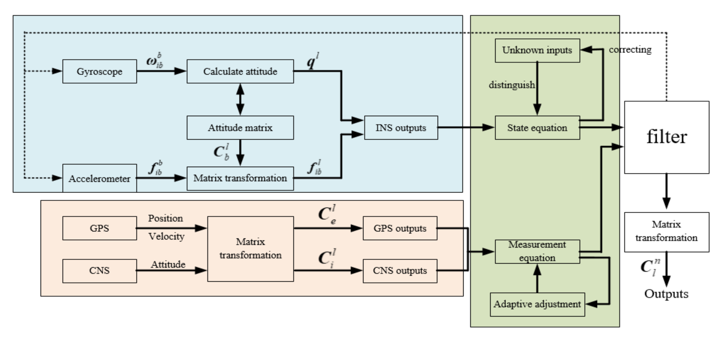
The overall scheme of the SINS/GPS/CNS integrated navigation system in launch inertial coordinate system designed in this paper is shown in Figure 1:

As shown in Figure 1, the inertial navigation solution module obtains the attitude angle from the output of the gyroscope and calculates the attitude quaternion to obtain the attitude transfer matrix from the body coordinate system to the launch inertial coordinate system. According to the attitude transfer matrix and the outputs of the accelerometer, the velocity and position calculation are performed. The position and velocity output of GPS in the earth fixed coordinate system is converted to launch the inertial coordinate system through the conversion matrix. The attitude output of CNS in the inertial coordinate system is converted to launch the inertial coordinate system through the conversion matrix.

According to the existing public data, aerospace vehicles are generally carried on rockets for launch, and rockets generally use the launch inertial coordinate system as the reference coordinate system for navigation calculation. After flying out of the atmosphere, the motion characteristics of aerospace vehicles are like those of on-orbit satellites, while on-orbit satellites generally use the inertial coordinate system as the reference coordinate system for navigation calculation. Therefore, this paper uses the launch inertial coordinate system as the reference coordinate system of the aerospace vehicle navigation system, which can unify the description of navigation parameters in different flight stages and reduce the conversion of navigation parameters in the calculation process to avoid the loss of accuracy.

Inertial Navigation Solution Module in Launch Inertial Coordinate System

In the strapdown inertial navigation system, the inertial device is fixed on the carrier, the angular rate output of the gyroscope is ${\mathit{\omega }}_{ib}^b$, ${\mathit{\omega }}_{lb}^b$ is the projection of the angular rate of the body coordinate system relative to the launch inertial coordinate system under the body coordinate system. Then ${\mathit{\omega }}_{lb}^b$ can be written as:

$${\mathit{\omega }}_{lb}^b={\mathit{\omega }}_{li}^b+{\mathit{\omega }}_{ib}^b$$

(1)

${\mathit{\omega }}_{li}^b$ is the projection of angular rate of inertial coordinate system relative to launch inertial coordinate system under the body coordinate system; ${\mathit{\omega }}_{ib}^b$ is the projection of the angular rate of the body coordinate system relative to the inertial coordinate system under the body coordinate system, where ${\mathit{\omega }}_{li}^b=0$, so:

$${\mathit{\omega }}_{lb}^b={\mathit{\omega }}_{ib}^b$$

(2)

For the attitude calculation module, a quaternion method can work in full attitude and a small amount of calculation is used to calculate the attitude. If the original three-dimensional output information of the gyroscope is expanded into a quaternion with the scalar part of 0 and the vector part of ${\mathit{\omega }}_{qi}$, it has the differential relationship with the quaternion $\mathit{q}$ corresponding to the attitude matrix as follows:

$$\dot{\mathit{q}}\left(t\right)=0.5\mathit{q}\left(t\right)\otimes {\mathit{\omega }}_{qi}$$

(3)

In Equation (3), $\otimes$ represents the multiplication of quaternions.

$$\dot{\mathit{q}}=\frac{1}{2}·\left[\begin{array}{cccc}{q}_0& -q_1& -q_2& -q_3\\ q_1& q_0& -q_3& q_2\\ q_2& q_3& q_0& -q_1\\ q_3& -q_2& q_1& q_0\end{array}\right]·\left[\begin{array}{c}0\\ {\mathit{\omega }}_{bx}\\ {\mathit{\omega }}_{by}\\ {\mathit{\omega }}_{bz}\end{array}\right]$$

(4)

The quaternion $\mathit{q}$ can be obtained by discretizing Equation (3) and calculating it by the Picard successive approximation method. After normalizing $\mathit{q}$, the conversion relationship ${\mathit{C}}_l^b$ between quaternions and attitude matrix can be calculated:

$${\mathit{C}}_l^b=\left[\begin{array}{ccc}{q}_0^2+q_1^2-q_2^2-q_3^2& 2\left(q_1{q}_2+q_0{q}_3\right)& 2\left(q_1{q}_3-q_0{q}_2\right)\\ 2\left(q_1{q}_2-q_0{q}_3\right)& q_0^2-q_1^2+q_2^2-q_3^2& 2\left(q_2{q}_3+q_0{q}_1\right)\\ 2\left(q_1{q}_3+q_0{q}_2\right)& 2\left(q_2{q}_3-q_0{q}_1\right)& q_0^2-q_1^2-q_2^2+q_3^2\end{array}\right]$$

(5)

From Equation (5), the expression for each attitude angle is:

$$\left\{\begin{array}{c}\gamma =-arctan\frac{t_{13}}{t_{33}}\\ \theta =arctan{t}_{23}\\ \psi =arctan\frac{t_{21}}{t_{22}}\end{array}\right.$$

(6)

In Equation (6), $t$ is equal to ${\mathit{C}}_l^b$.

In the strapdown inertial navigation system, the inertial device is directly fixed to the carrier, the accelerometer output is ${\mathit{f}}_{ib}^b$, represents the vector formed by the acceleration of the body coordinate system relative to the inertial coordinate system in the axial component of the body coordinate system. Then the accelerometer value ${\mathit{f}}_{ib}^l$ under launch inertial coordinate system can be obtained as:

$${\mathit{f}}_{ib}^l={\mathit{C}}_b^l{\mathit{f}}_{ib}^b$$

(7)

In Equation (7), ${\mathit{C}}_b^l$ is the attitude conversion matrix of the launch inertial system relative to the body coordinate system;

From Equation (7), the specific force equation under the launch inertial system can be written as:

$${\mathit{f}}_{ib}^l=\dot{\mathit{v}}-{\mathit{C}}_i^l\mathit{G}$$

(8)

In Equation (8), $\mathit{v}$ is the velocity value in launch inertial coordinate system; $\mathit{G}$ is the universal gravitation force of the Earth; ${\mathit{C}}_i^l$ is the attitude transition matrix of the launch inertial system relative to the inertial system.

In the launch inertial coordinate system, the position under the launch inertial coordinate system can be calculated by integrating the navigation velocity:

$$\dot{\mathit{p}}=\mathit{v}$$

(9)

In Equation (9), $\mathit{v}$ is the velocity vector.

The navigation model in launch inertial coordinate system can be written as:

$$\left\{\begin{array}{l}\dot{\mathit{q}}=0.5\mathit{q}\otimes {\mathit{\omega }}_{lb}^b\\ \dot{\mathit{v}}={\mathit{C}}_b^l·{\mathit{f}}^b+{\mathit{C}}_i^l·{\mathit{G}}^i\\ \dot{\mathit{p}}=\mathit{v}\end{array}\right.$$

(10)

Among them, $\mathit{q}$ is the quaternion; ${\mathit{C}}_b^l$ is the transfer matrix from the body coordinate system to the launch inertial coordinate system; ${\mathit{f}}^b$ is the specific force of the accelerometer in the body coordinate system; ${\mathit{C}}_i^l$ is the transfer matrix from the inertial coordinate system to the launch inertial coordinate system; ${\mathit{G}}^i$ is the gravitational force in the inertial coordinate system; $\mathit{p}$ is the position vector.

According to Equation (10), the error equations of navigation information including attitude quaternion, velocity and position of the aerospace vehicle in launch inertial coordinate system can be derived. The differential equations are as follows:

$$\left\{\begin{array}{c}\delta {\dot{\mathit{q}}}_{13}=-\left[{\widehat{\mathit{\omega }}}_{ib}^b\times \right]\cdot \mathit{\delta }{q}_{13}+0.5\cdot \delta \mathit{W}\\ \delta \dot{\mathit{v}}=-2{\mathit{C}}_b^l\cdot \left[{\widehat{\mathit{f}}}^b\times \right]\cdot \delta {\mathit{q}}_{13}+{\mathit{C}}_b^l\cdot {\mathbf{\nabla }}_a+{\mathit{C}}_b^l\cdot \delta \mathit{G}\\ \delta \dot{\mathit{p}}=\delta \mathit{v}\end{array}\right.$$

(11)

In Equation (11), $\delta {\mathit{q}}_{13}$ is the vector part of $\delta \mathit{q}$; $\delta \mathit{v}$ is the velocity error vector; $\delta \mathit{p}$ is the position error vector; $\delta \mathit{W}$ is the gyro noise; ${\mathbf{\nabla }}_a$ is the accelerometer error; $\delta \mathit{G}$ is the gravity error; $\left[{\widehat{\mathit{\omega }}}_{ib}^b\times \right]$ represent the symmetric matrix of ${\widehat{\mathit{\omega }}}_{ib}^b$; $\left[{\widehat{\mathit{f}}}^b\times \right]$ represent the symmetric matrix of ${\mathit{f}}_{ib}^b$.

2.2. Matrix Transformation of Launch Inertial Coordinate System

Unlike aero-planes, the larger flight envelope of the aerospace vehicle means that the simplified model of the Earth used by traditional inertial navigation algorithms in the geographic coordinate system is no longer suitable for its navigation system. Therefore, this paper discusses navigation algorithms under launch inertial system with an accurate model of the Earth.

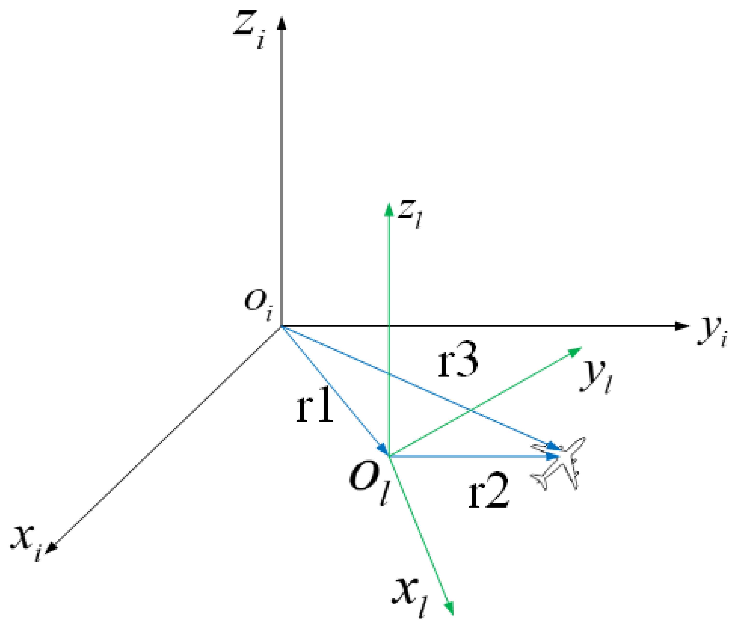
Among them, the origin of the launch inertial coordinate system is taken at the launch point of the aerospace vehicle, and its coordinate axis direction is defined by the aerospace vehicle at the launch time. The y-axis is the vertical line passing the launch point, and upward is positive. The x-axis is perpendicular to the y-axis at the launch time. The z-axis, the x-axis and the y-axis constitute a right-handed rectangular coordinate system. The conversion relationship between the launch inertial coordinate system and the J2000 inertial coordinate system is shown in the Figure 2:

In order to calculate the transfer matrix ${\mathit{C}}_i^l$ from the launch inertial coordinate system to the inertial coordinate system, the first step is to calculate ${\mathit{C}}_n^l$ (the transfer matrix from the geographic system (launch origin) to launch inertial coordinate system), ${\mathit{C}}_e^n$ (the transfer matrix from the Earth Fixed coordinate system to geographic coordinate system (launch origin)), ${\mathit{C}}_i^e$ (the transfer matrix from the inertial coordinate system to Earth Fixed coordinate system), where:

$${\mathit{C}}_l^n=\left[\begin{array}{ccc}1\hfill & 0& 0\\ 0\hfill & cos\left(-90\right)& sin\left(-90\right)\\ 0\hfill & -sin\left(-90\right)& cos\left(-90\right)\end{array}\right]·\left[\begin{array}{ccc}cos\left(-\left(90-A\right)\right)\hfill & 0& -sin\left(-\left(90-A\right)\right)\\ 0& 1& 0\\ sin\left(-\left(90-A\right)\right)\hfill & 0& cos\left(-\left(90-A\right)\right)\end{array}\right]$$

(12)

In Equation (12), $A$ is the launch deflection angle.

$${\mathit{C}}_n^e=\left[\begin{array}{ccc}cos\left(-\left(90+\lambda \right)\right)& sin\left(-\left(90+\lambda \right)\right)& 0\\ -sin\left(-\left(90+\lambda \right)\right)& cos\left(-\left(90+\lambda \right)\right)& 0\\ 0& 0& 1\end{array}\right]·\left[\begin{array}{ccc}1& 0& 0\\ 0& cos\left(-\left(90-\phi \right)\right)& sin\left(-\left(90-\phi \right)\right)\\ 0& -sin\left(-\left(90-\phi \right)\right)& cos\left(-\left(90-\phi \right)\right)\end{array}\right]$$

(13)

The conversion from the Protocol geographic coordinate system to the WGS84 coordinate system needs to consider the influence of polar motion, then:

$${\mathit{C}}_1^e=\left[\begin{array}{ccc}1& 0& {\mathit{x}}_p\\ 0& 1& 0\\ {\mathit{x}}_p& 0& 1\end{array}\right]·\left[\begin{array}{ccc}1& 0& 0\\ 0& 1& -{\mathit{y}}_p\\ 0& {\mathit{y}}_p& 1\end{array}\right]$$

(14)

In Equation (14), $\left({\mathit{x}}_p,{\mathit{y}}_p\right)$ is the coordinates of the pole.

When converting from an instantaneous ground-fixed coordinate system to an instantaneous true equatorial geocentric celestial coordinate system, the time angle of the vernal equinox needs to be considered, then:

$${\mathit{C}}_2^1=\left[\begin{array}{ccc}cos\theta & sin\theta & 0\\ -sin\theta & cos\theta & 0\\ 0& 0& 1\end{array}\right]$$

(15)

$$\mathit{\theta }=\stackrel{-}{\theta }+\Delta \varphi cos\tilde{\epsilon }$$

(16)

$\overline{\theta }$ is Greenwich Mean Sidereal Time.

Conversion from the instantaneous horizontal celestial coordinate system to the instantaneous true celestial coordinate system:

$${\mathit{C}}_3^2=\left[\begin{array}{ccc}1& 0& 0\\ 0& cos\tilde{\epsilon }& -sin\tilde{\epsilon }\\ 0& sin\tilde{\epsilon }& cos\tilde{\epsilon }\end{array}\right]\left[\begin{array}{ccc}cos\varphi & -sin\varphi & 0\\ sin\varphi & cos\varphi & 0\\ 0& 0& 1\end{array}\right]\left[\begin{array}{ccc}1& 0& 0\\ 0& cos\overline{\epsilon }& sin\overline{\epsilon }\\ 0& -sin\overline{\epsilon }& cos\overline{\epsilon }\end{array}\right]$$

(17)

In Equation (17),

• mean obliquity:

  $$\overline{\epsilon }={84381}^{″}.448-{46}^{″}.815·Tu-0^{″}.00059·T{u}^2+0.001813·T{u}^3$$

  (18)
• nutation in obliquity:

  $$\Delta \epsilon =9^{″}.2025cos\Omega +0^{″}.5736·cos(2L)$$

  (19)
• true ecliptic obliquity:

  $$\tilde{\epsilon }=\overline{\epsilon }+\Delta \epsilon$$

  (20)
• nutation of longitude:

  $$\Delta \varphi =-{17}^{″}.1996sin\Omega -1^{″}.3187·sin(2L)$$

  (21)
• right ascension of moon ascending node:

  $$\Omega =125.04-0.052954·JD$$

  (22)
• mean longitude of the sun:

  $$L=280.47-0.98565·JD$$

  (23)

The conversion from the J2000 coordinate system to the instantaneous horizontal celestial coordinate system needs to consider the effect of precession, then:

$${\mathit{C}}_i^3=\left[\begin{array}{ccc}cos{Z}_A& -sin{Z}_A& 0\\ sin{Z}_A& cos{Z}_A& 0\\ 0& 0& 1\end{array}\right]\left[\begin{array}{ccc}cos{\theta }_A& 0& -sin{\theta }_A\\ 0& 1& 0\\ sin{\theta }_A& 0& cos{\theta }_A\end{array}\right]\left[\begin{array}{ccc}cos{\varsigma }_A& -sin{\varsigma }_A& 0\\ sin{\varsigma }_A& cos{\varsigma }_A& 0\\ 0& 0& 1\end{array}\right]$$

(24)

In Equation (24): $Tu$ is Julian Day, and ${\mathit{\varsigma }}_A$, ${\mathit{Z}}_A$, ${\mathit{\theta }}_A$ are three Euler angles in the equatorial plane.

Then the matrix ${\mathit{C}}_i^e$ established based on the accurate earth model from the inertial coordinate system to the ground-fixed coordinate system is:

$${\mathit{C}}_i^e={\mathit{C}}_1^e·{\mathit{C}}_2^1·{\mathit{C}}_3^2·{\mathit{C}}_i^3$$

(25)

Since the orbital height of ASV is about 300 km, it can be roughly regarded as a low-earth orbit satellite, which means that the factor that has the greatest influence on the gravitational field is the ellipticity of the earth. Therefore, the gravity field model is as follows.

$$\mathit{G}=\left[\begin{array}{c}-\frac{\mu x}{r^3}\left[1-J_2{\left(\frac{{\mathit{R}}_e}{r}\right)}^2\left(7.5\frac{z^2}{r^2}-1.5\right)\right]\\ -\frac{\mu y}{r^3}\left[1-J_2{\left(\frac{{\mathit{R}}_e}{r}\right)}^2\left(7.5\frac{z^2}{r^2}-1.5\right)\right]\\ -\frac{\mu z}{r^3}\left[1-J_2{\left(\frac{{\mathit{R}}_e}{r}\right)}^2\left(7.5\frac{z^2}{r^2}-4.5\right)\right]\end{array}\right]$$

(26)

In the above equation, $x,y,z$ are the carrier position of aerospace vehicles in the geocentric inertial coordinate system; $J_2=1.08263\times {10}^{-3}$, which is the second-order harmonic coefficient; $\mu =3.986\times {10}^{14} {\mathrm{m}}^3{\mathrm{s}}^{-2}$, which is the gravitational constant; $R_e$ = 6,378,137 m, which is the equatorial radius; $r$ is the distance from the carrier to the center of the Earth. The accurate gravity model derived from Equation (16) is brought into Equation (11) to improve the modeling accuracy of system state quantity.

2.3. Establishing the State Equation and Measurement Equation for Integrated Navigation System

After establishing the strapdown inertial navigation system model in the launch inertial coordinate system, this paper directly establishes the state model and observation model of the SINS/GPS/CNS integrated navigation system in the launch inertial system.

The system state equation is:

$$\dot{\mathit{X}}\left(t\right)=\mathit{A}\left(t\right)\mathit{X}\left(t\right)+\mathit{B}\left(t\right)\mathit{W}\left(t\right)$$

(27)

In Equation (27), $\mathit{A}\left(t\right)$ is the system matrix;

$$\mathit{A}\left(t\right)=\left[\begin{array}{ccccc}{0}_{3\times 3}& 0_{3\times 3}& 0_{3\times 3}& {\mathit{C}}_b^l& 0_{3\times 3}\\ {\mathit{F}}_a& 0_{3\times 3}& {\mathit{F}}_b& 0_{3\times 3}& {\mathit{C}}_b^l\\ 0_{3\times 3}& {\mathit{I}}_{3\times 3}& 0_{3\times 3}& 0_{3\times 3}& 0_{3\times 3}\\ 0_{3\times 3}& 0_{3\times 3}& 0_{3\times 3}& 0_{3\times 3}& 0_{3\times 3}\\ 0_{3\times 3}& 0_{3\times 3}& 0_{3\times 3}& 0_{3\times 3}& 0_{3\times 3}\end{array}\right]$$

(28)

In Equation (28), ${\mathit{F}}_a$ is an antisymmetric matrix composed of apparent acceleration; ${\mathit{F}}_b$ is determined by the partial derivative of gravitational acceleration to position. $\mathit{B}\left(t\right)$ is the system noise matrix;

$$\mathit{B}\left(t\right)=\left[\begin{array}{cc}{\mathit{C}}_b^l& 0_{3\times 3}\\ 0_{3\times 3}& {\mathit{C}}_b^l\\ 0_{3\times 3}& 0_{3\times 3}\\ 0_{3\times 3}& 0_{3\times 3}\\ 0_{3\times 3}& 0_{3\times 3}\end{array}\right]$$

(29)

$\mathit{X}\left(t\right)$ is the state vector; $\mathit{W}\left(t\right)$ is the system noise vector; Combined Equation (10) and Equation (27), State quantity $\mathit{X}$ is:

$$\mathit{X}=\left[\begin{array}{ccccccccccccccc}\mathit{\delta }{\mathit{q}}_1& \mathit{\delta }{\mathit{q}}_2& \mathit{\delta }{\mathit{q}}_3& \mathit{\delta }{\mathit{p}}_x& \mathit{\delta }{\mathit{p}}_y& \mathit{\delta }{\mathit{p}}_z& \mathit{\delta }{\mathit{v}}_x& \mathit{\delta }{\mathit{v}}_y& \mathit{\delta }{\mathit{v}}_z& {\mathit{\omega }}_{rx}& {\mathit{\omega }}_{ry}& {\mathit{\omega }}_{rz}& {\mathit{f}}_{rx}& {\mathit{f}}_{ry}& {\mathit{f}}_{rz}\end{array}\right]$$

(30)

In the above equation, $\mathit{\delta }{\mathit{q}}_1,\mathit{\delta }{\mathit{q}}_2,\mathit{\delta }{\mathit{q}}_3$ are three-dimensional vector error part of attitude quaternion; $\mathit{\delta }{\mathit{p}}_x,\mathit{\delta }{\mathit{p}}_y,\mathit{\delta }{\mathit{p}}_z$ are position error; $\mathit{\delta }{\mathit{v}}_x,\mathit{\delta }{\mathit{v}}_y,\mathit{\delta }{\mathit{v}}_z$ are velocity error; ${\mathit{\omega }}_{rx},{\mathit{\omega }}_{ry},{\mathit{\omega }}_{rz}$ are gyro random walk error; ${\mathit{f}}_{rx},{\mathit{f}}_{ry},{\mathit{f}}_{rz}$ are accelerometer random walk error

The system noise vector $\mathit{W}$ is:

$$\mathit{W}=\left[\begin{array}{ccccccccc}{\mathit{\omega }}_{\epsilon x}& {\mathit{\omega }}_{\epsilon y}& {\mathit{\omega }}_{\epsilon z}& {\mathit{\omega }}_{nx}& {\mathit{\omega }}_{ny}& {\mathit{\omega }}_{nz}& {\mathit{f}}_{nx}& {\mathit{f}}_{ny}& {\mathit{f}}_{nz}\end{array}\right]$$

(31)

In the integrated navigation system observation equation, the position measurement information output from the GPS and the attitude measurement information output from the CNS are regarded as the observation vector. Then the observation vector of SINS/CNS subsystem can be written as:

$${\mathit{Z}}_C\left(t\right)={\mathit{H}}_a\left(t\right)\mathit{X}\left(t\right)+{\mathit{r}}_{\eta }$$

(32)

In Equation (32), ${\mathit{r}}_{\eta }$ is the noise matrix measured by the star sensor.

$${\mathit{H}}_a{\left(t\right)}_{3\times 15}={\left[I_{3\times 3}{0}_{3\times 12}\right]}_{3\times 15}$$

(33)

Similarly: the observation vector of the SINS/GPS subsystem can be written as:

$${\mathit{Z}}_G\left(t\right)={\mathit{H}}_p\left(t\right)\mathit{X}\left(t\right)+{\mathit{r}}_{\epsilon }$$

(34)

In Equation (34), ${\mathit{r}}_{\epsilon }$ is the noise matrix measured by the GPS.

$${\mathit{H}}_p{\left(t\right)}_{3\times 15}={\left[0_{3\times 3 }{I}_{3\times 3 }{0}_{3\times 9}\right]}_{3\times 15}$$

(35)

From Equations (33) and (35), the SINS/GPS/CNS integrated navigation system observation vector can be written as:

$$\mathit{H}{\left(t\right)}_{3\times 15}={\left[I_{3\times 3 }{I}_{3\times 3 }{0}_{3\times 9}\right]}_{3\times 15}$$

(36)

3. Multi-Layer Fault-Tolerant Robust Filtering Algorithm

After the model of the strapdown inertial navigation system and integrated navigation system in the launch inertial coordinate system have been established, the integrated navigation filtering algorithm needs to be further researched. The aerospace vehicle must perform cross-airspace, highly dynamic and wide-range missions, so its navigation system will be affected by many uncertainties, which makes it impossible to accurately model the navigation system errors, and the statistical characteristics of the navigation system noise are also difficult to be obtained. In this paper, the above situation can be regarded as the existence of unknown inputs in the state equation of the navigation system, which leads to the performance limitation of the traditional linear Kalman filter. In addition, the aerospace vehicle navigation system is equipped with many sensors and the complex flight environment may cause some measurement sensors to fail, such as satellite signals are interfered with, the star sensor cannot be effectively calculated due to stargazing conditions, etc., which leads to a decrease in the accuracy of the navigation system. Therefore, it is necessary to identify, estimate and compensate the unknown inputs of the navigation system state equation, as well as to perform real-time fault diagnosis, isolation and reconstruction of the measurement information to improve the accuracy and robustness of the navigation system at multiple levels.

3.1. Design of Robust Fault Tolerant Filtering Architecture

In order to improve the fault tolerance and robustness of the navigation system filter, it is necessary to compensate and correct errors caused by various unknown factors such as an inaccurate system model and measurement-sensor failures since the Kalman filter algorithm can only obtain optimal estimates of state quantities when both the structural parameters and the statistical properties of the noise of the dynamic system are accurate. When the relevant parameters are inaccurate, the Kalman filter accuracy decreases or even diverges. The model error of the system usually affects the output of the system. For this reason, A.P. Sage and G.W. Husa proposed the adaptive filtering algorithm, and its method currently is mainly used to estimate the variance of the measurement noise. Meanwhile, it cannot eliminate the influence of the unknown inputs in the state equation, which leads to a large filtering error.

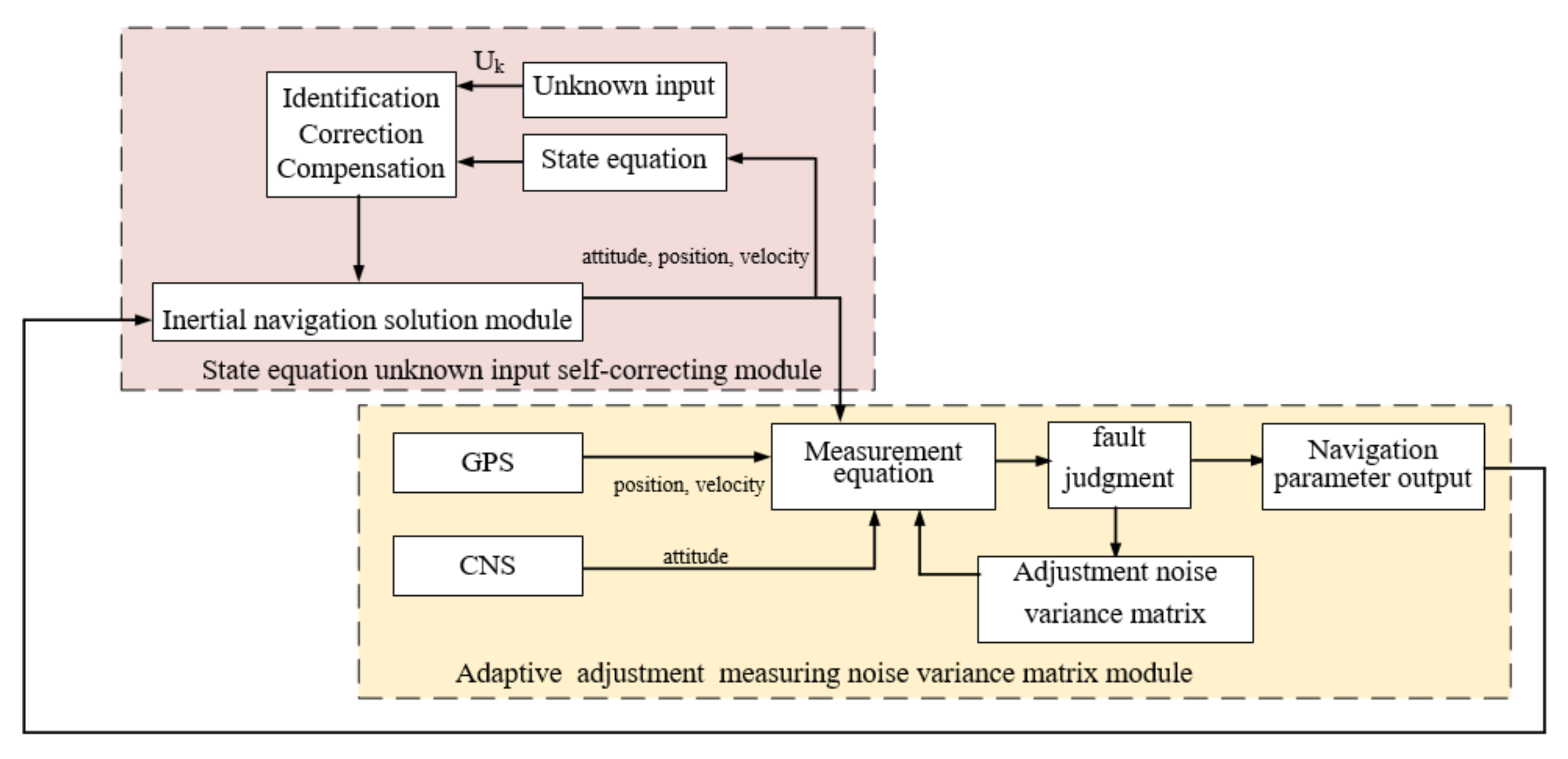
Therefore, this section proposes a multi-layer robust fault-tolerant filter design method, as shown in Figure 3.

Firstly, we use the state equation unknown-inputs self-correction module to estimate and compensate the unknown input in the state equation automatically. Meanwhile, the measurement noise-variance matrix adaptive module is used to detect the failure of the measurement information, and to adapt the measurement noise-variance matrix. Combining the above two modules to construct a multi-layer, fault-tolerant robust filter structure can improve the robustness and accuracy of the aerospace vehicle navigation system in a large dynamic environment.

Self-Recognition Algorithm for Unknown Input of State Equation

When the integrated navigation system model is inconsistent with the filter model or the statistical characteristics of the system noise are unknown due to the large dynamic flight of aerospace vehicle, this is reflected in the existence of unknown inputs to the system state equation. Therefore, it needs to be identified, compensated and corrected to improve the navigation system accuracy.

From Equations (27) and (32), the system equation can be written as:

$${\mathit{X}}_{k+1}={\mathit{f}}_k\left({\mathit{X}}_k\right)+{\mathit{U}}_k+{\mathit{W}}_k$$

(37)

$${\mathit{Z}}_k={\mathit{h}}_k\left({\mathit{X}}_k\right)+{\mathit{V}}_k$$

(38)

In Equations (37) and (38), The definitions of ${\mathit{f}}_k$, ${\mathit{h}}_k$, ${\mathit{W}}_k$ and ${\mathit{V}}_k$ are the same as in the previous chapter, and ${\mathit{U}}_k$ is the unknown input in the state equation.

Since the filter update time interval is small enough, the unknown input of the adjacent interval often changes little [25], so that the unknown input ${\mathit{U}}_k$ can be estimated and when the sampling period $k\ge 3$, the unknown input ${\mathit{U}}_k$ can be approximately expressed as:

$${\mathit{U}}_k\approx {\mathit{U}}_{k-1}$$

(39)

The initial estimate of the state unknown input ${\mathit{U}}_k$ is:

$${\widehat{\mathit{U}}}_k^{\left(0\right)}={\widehat{\mathit{X}}}_k-{\mathit{f}}_{k-1}\left({\mathit{X}}_{k-1}\right)$$

(40)

In Equation (40), it is necessary to distinguish ${\widehat{\mathit{U}}}_k^{\left(0\right)}$ due to unknown inputs or accidental errors. Therefore:

$${\widehat{\mathit{U}}}_k,j=\left\{\begin{array}{c}0, \mathrm{if} \left|{\widehat{\mathit{U}}}_{k,j}^{\left(0\right)}\right|<c{\sigma }_{k,j}\\ {\widehat{\mathit{U}}}_{k,j}^{\left(0\right)}, \mathrm{if} \left|{\widehat{\mathit{U}}}_{k,j}^{\left(0\right)}\right|\ge c{\sigma }_{k,j}\end{array}\right.j=1,2,\cdots ,l$$

(41)

In Equation (41), the ${\widehat{\mathit{U}}}_k,j$ and ${\widehat{\mathit{U}}}_{k,j}^{\left(0\right)}$ are respectively the $j\mathrm{th}$ component of ${\widehat{\mathit{U}}}_k$ and ${\widehat{\mathit{U}}}_k^{\left(0\right)}$, ${\mathit{\sigma }}_{k,j}$ is written as:

$${\mathit{\sigma }}_{k,j}=\sqrt{{\mathit{Q}}_k\left(j,j\right)} j=1,2,\cdots ,l$$

(42)

At this point, the Kalman one-step prediction formula can be written as:

$${\widehat{\mathit{X}}}_{\left(k|k-1\right)}={\mathit{F}}_{k-1}{\widehat{\mathit{X}}}_{k-1}+{\widehat{\mathit{U}}}_{k-1}$$

(43)

The one-step prediction covariance matrix can be written as:

$${\mathit{P}}_{\left(k|k-1\right)}={\mathit{F}}_{k-1}{\mathit{P}}_{k-1}{\mathit{F}}_{k-1}^T+{\mathit{Q}}_{k-1}+{\mathsf{\Theta }}_{k-1}+{\mathsf{\Theta }}_{k-1}^T+{\mathsf{\Theta }}_{k-1}^{*}$$

(44)

In Equation (44), ${\mathsf{\Theta }}_{k-1}$ is written as:

$${\mathsf{\Theta }}_{k-1}={\mathit{F}}_{k-1}\left[{\mathit{P}}_{k-1}-{\mathit{S}}_{k-1}{\mathit{F}}_{k-2}^T-\left(I-{\mathit{K}}_{k-1}{\mathit{H}}_{k-1}\right){\mathit{Q}}_{k-2}\right]{\mathit{T}}_{k-1}$$

(45)

$${\mathsf{\Theta }}_{k-1}^{*}={\mathit{T}}_{k-1}\left[\begin{array}{c}{\mathit{P}}_{k-1}+{\mathit{F}}_{k-2}{\mathit{P}}_{k-2}{\mathit{F}}_{k-2}^T+{\mathit{Q}}_{k-2}-{\mathit{S}}_{k-1}{\mathit{F}}_{k-2}^T-\left(I-{\mathit{K}}_{k-1}{\mathit{H}}_{k-1}\right){\mathit{Q}}_{k-2} -\\ {\mathit{F}}_{k-2}{\mathit{S}}_{k-1}^T-{\mathit{Q}}_{k-2}^T{\left(I-{\mathit{K}}_{k-1}{\mathit{H}}_{k-1}\right)}^T\end{array}\right]{\mathit{T}}_{k-1}$$

(46)

In above equation, the $I$ is the unit matrix, ${\mathit{T}}_{k-1}$ is the diagonal matrix where the elements in the $l$th row and the $l$th column are 1 when ${\widehat{\mathit{U}}}_{k-1},j\ne 0$, and the other non-diagonal elements are all 0. When ${\widehat{\mathit{U}}}_{k-1},j=0$, the element in the $l$th row and the $l$th column is 0, and the other non-diagonal elements are all 0 diagonal matrices. ${\mathit{S}}_{k-1}$ is:

$${\mathit{S}}_{k-1}=\left(I-{\mathit{K}}_{k-1}{\mathit{H}}_{k-1}\right)\left\{{\mathit{F}}_{k-2}{\mathit{P}}_{k-2}+{\mathit{T}}_{k-2}\left[\begin{array}{c}{\mathit{P}}_{k-2}-{\mathit{F}}_{k-3}{\mathit{S}}_{k-2}^T -\\ {\mathit{Q}}_{k-3}{\left(I-{\mathit{K}}_{k-2}{\mathit{H}}_{k-2}\right)}^T\end{array}\right]\right\}$$

(47)

$$S_1=P_1$$

(48)

State estimation:

$${\widehat{\mathit{X}}}_k={\widehat{\mathit{X}}}_{\left(k|k-1\right)}+{\mathit{K}}_k\left({\mathit{Z}}_k-{\mathit{H}}_k{\widehat{\mathit{X}}}_{\left(k|k-1\right)}\right)$$

(49)

The covariance matrix for the state estimation is:

$${\mathit{P}}_k=\left(I-{\mathit{K}}_k{\mathit{H}}_k\right){\mathit{P}}_{\left(k|k-1\right)}$$

(50)

The filtering gain is:

$${\mathit{K}}_k={\mathit{P}}_{\left(k|k-1\right)}{\mathit{H}}_k^T{\left({\mathit{H}}_k{\mathit{P}}_{\left(k|k-1\right)}{\mathit{H}}_k^T+{\mathit{R}}_k\right)}^{-1}$$

(51)

3.2. Adaptive Algorithm for Measuring Noise Variance Matrix

During the actual flight of the aerospace vehicle, as it needs to go through the launch phases, in-orbit phases, and re-entry phases, it faces an extremely complex flight environment and the navigation sensors are prone to malfunction, such as the satellite navigation system being interfered with and unable to provide position and velocity information normally, or the star sensor cannot calculate the attitude of the aerospace vehicle properly. As a result, it is necessary to perform fault diagnosis, isolation and reconstruction of the measurement information obtained by the navigation sensors.

3.2.1. Residual Mismatch Degree Detection

From the analysis of the content in the previous section, the prediction error of the system measurement can be written as:

$${\tilde{\mathit{Z}}}_{\left(k|k-1\right)}={\mathit{H}}_k{\tilde{\mathit{X}}}_{\left(k|k-1\right)}+{\mathit{V}}_k$$

(52)

Taking the variances of both sides of Equation (52) simultaneously and shifting the terms gives the expression for the measurement noise variance matrix that can be obtained as:

$${\mathit{R}}_k=E\left[{\tilde{\mathit{Z}}}_{\left(k|k-1\right)}{\tilde{\mathit{Z}}}_{\left(k|k-1\right)}^T\right]-{\mathit{H}}_k{\mathit{P}}_{\left(k|k-1\right)}{\mathit{H}}_k^T$$

(53)

In above equation, the $E\left[{\tilde{\mathit{Z}}}_{\left(k|k-1\right)}{\tilde{\mathit{Z}}}_{\left(k|k-1\right)}^T\right]$ is the lumped average of the random sequence. In practical applications, the traditional adaptive filtering adopts the equal weighted recursive estimation method [26], which will gradually lose the adaptive effect after long-time filtering. Therefore, this paper adopts the exponential fading memory weighted average method to ensure the robustness of the navigation system under long-time working conditions. The time average is used instead, and then the exponential fading memory weighted average of ${\mathit{R}}_k$ can be written as:

$${\tilde{\mathit{R}}}_k=\left(1-{\varrho }_k\right){\tilde{\mathit{R}}}_{k-1}+{\varrho }_k\left({\tilde{\mathit{Z}}}_{\left(k|k-1\right)}{\tilde{\mathit{Z}}}_{\left(k|k-1\right)}^T-{\mathit{H}}_k{\mathit{P}}_{\left(k|k-1\right)}{\mathit{H}}_k^T\right)$$

(54)

In above equation, ${\varrho }_k$ can be written as:

$${\varrho }_k=\frac{{\mathit{\varrho }}_{k-1}}{{\mathit{\varrho }}_{k-1}+\tau }$$

(55)

In Equation (55), ${\varrho }_0=1$, $\tau$ is the fading factor.

When the system is modelled accurately, the $E\left[{\tilde{\mathit{Z}}}_{\left(k|k-1\right)}{\tilde{\mathit{Z}}}_{\left(k|k-1\right)}^T\right]$ can be written as:

$$E\left[{\tilde{\mathit{Z}}}_{\left(k|k-1\right)}{\tilde{\mathit{Z}}}_{\left(k|k-1\right)}^T\right]={\mathit{H}}_k\left(\begin{array}{c}{\Phi }_{\left(k|k-1\right)}{\mathit{P}}_{k-1}{\Phi }_{\left(k|k-1\right)}^T +\\ {\Gamma }_{\left(k|k-1\right)}{\mathit{Q}}_{k-1}{\Gamma }_{\left(k|k-1\right)}^T\end{array}\right){\mathit{H}}_k^T+{\mathit{R}}_k$$

(56)

In Equation (56), $\Phi$ is the Jacobian matrix of $\mathit{f}$.

Combining Equations (55) and (56) can be written as:

$${\widehat{\mathbf{B}}}_k=\left(1-{\varrho }_k\right){\tilde{\mathbf{B}}}_{k-1}+{\varrho }_k{\tilde{\mathit{Z}}}_{\left(k|k-1\right)}{\tilde{\mathit{Z}}}_{\left(k|k-1\right)}^T$$

(57)

If the quantity measurement ${\mathit{Z}}_k$ has large fluctuations, let

$$E\left[{\tilde{\mathit{Z}}}_{\left(k|k-1\right)}{\tilde{\mathit{Z}}}_{\left(k|k-1\right)}^T\right]={\widehat{\Lambda }}_k$$

(58)

then:

$$tr\left({\widehat{\Lambda }}_k\right)\ll tr\left({\widehat{\mathbf{B}}}_k\right)$$

(59)

From Equation (59), it can be judged whether the quantity measurement ${\mathit{Z}}_k$ is faulty.

3.2.2. Adaptively Adjust Measurement Noise Variance

After detecting the failure of the measurement information, the ${\mathit{P}}_{\left(k|k-1\right)}$ in the Kalman filter equation have been adjusted adaptively.

Adjust the mean square error matrix ${\mathit{P}}_{k-1}$ by Equations (38) and (56), then:

$${\widehat{\mathbf{B}}}_k-{\mathit{H}}_k{\Gamma }_{\left(k|k-1\right)}{\mathit{Q}}_{k-1}{\Gamma }_{\left(k|k-1\right)}^T{\mathit{H}}_k^T-{\mathit{R}}_k={\mathit{H}}_k{\Phi }_{\left(k|k-1\right)}\left({\lambda }_k{\mathit{P}}_{k-1}\right){\Phi }_{\left(k|k-1\right)}^T{\mathit{H}}_k^T$$

(60)

In Equation (60), ${\lambda }_k$ is the proportionality coefficient, which can be written as:

$${\lambda }_k=\frac{tr\left({\mathit{N}}_k\right)}{tr\left({\mathit{M}}_k\right)}$$

(61)

In Equation (61), $tr$ is the matrix tracing operation, ${\mathit{N}}_k$ can be written as:

$${\mathit{N}}_k={\widehat{\mathbf{B}}}_k-{\mathit{H}}_k{\Gamma }_{\left(k|k-1\right)}{\mathit{Q}}_{k-1}{\Gamma }_{\left(k|k-1\right)}^T{\mathit{H}}_k^T-{\mathit{R}}_k$$

(62)

${\mathit{M}}_k$ can be written as:

$${\mathit{M}}_k={\mathit{H}}_k{\Phi }_{\left(k|k-1\right)}\left({\lambda }_k{\mathit{P}}_{k-1}\right){\Phi }_{\left(k|k-1\right)}^T{\mathit{H}}_k^T$$

(63)

Since ${\lambda }_k$ should not be less than 1, it is necessary to judge ${\lambda }_k$:

$${\lambda }_k=\left\{\begin{array}{c}1 {\lambda }_k<1\\ \frac{tr\left({\mathit{N}}_k\right)}{tr\left({\mathit{M}}_k\right)} {\lambda }_k\ge 1\end{array}\right.$$

(64)

At this point, ${\mathit{P}}_{\left(k|k-1\right)}$ in the Kalman filter equation becomes:

$${\mathit{P}}_{\left(k|k-1\right)}={\Phi }_{\left(k|k-1\right)}\left({\lambda }_k{\mathit{P}}_{k-1}\right){\Phi }_{\left(k|k-1\right)}^T+{\Gamma }_{k-1}{\mathit{Q}}_{k-1}{\Gamma }_{\mathrm{k}-1}^T$$

(65)

Combining Equations (49)–(51) and (65), the multi-layer robust fault-tolerant filtering equation can be obtained.

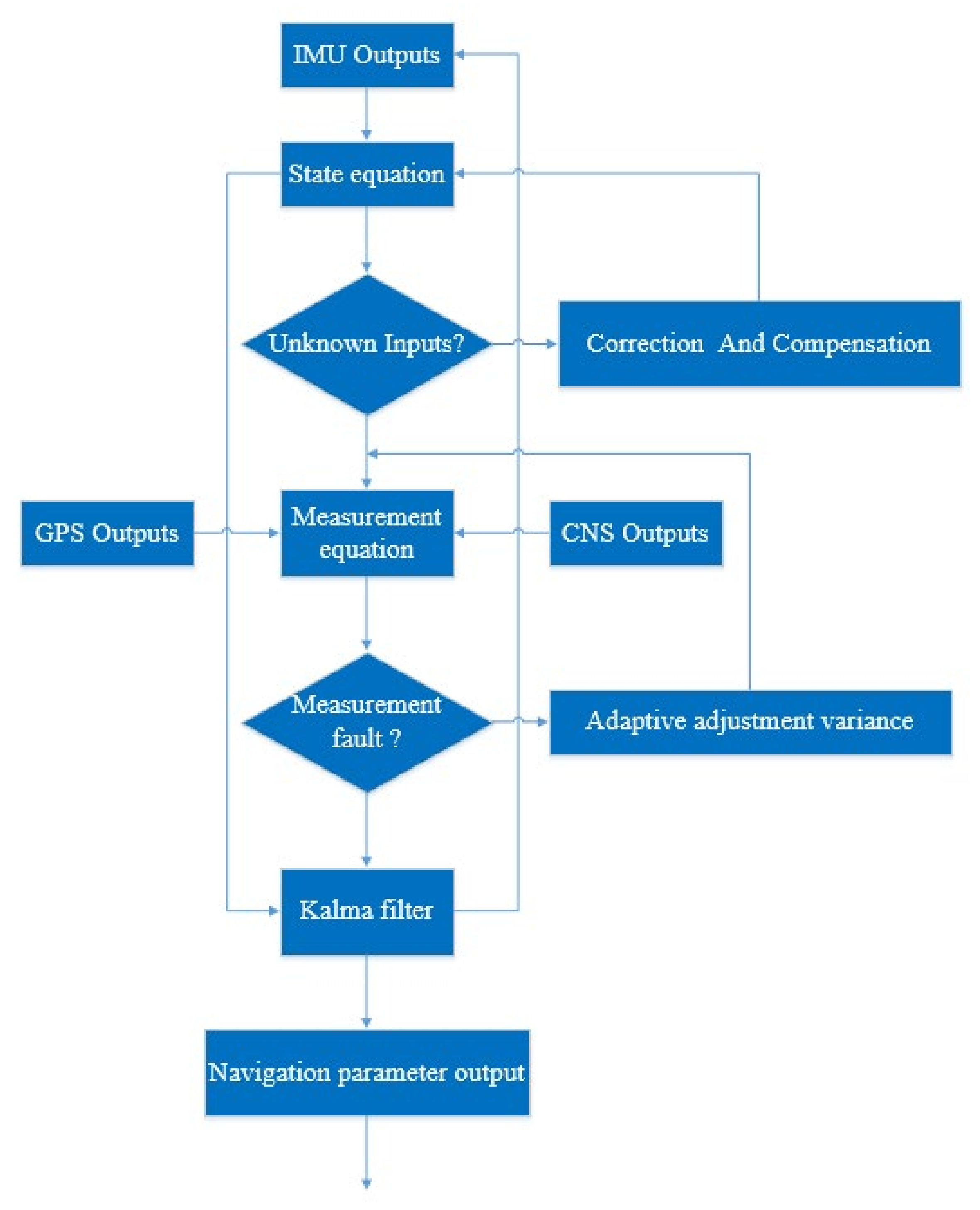
The flow chart of the algorithm is shown in Figure 4:

4. Simulation and Verification

In this section, Monte Carlo simulation methods are used to simulate the KF algorithm, the UKF algorithm and the RF algorithm in this paper, and the root mean square error of RF algorithm, KF algorithm and UKF algorithm are respectively calculated. The simulation software is Matlab R2020b. Rotational angular velocity of the Earth is $7.292115\times {10}^{-5 }\mathrm{rad}/\mathrm{s}$, Earth oblateness is $1/298.257$.

4.1. Simulation Condition Setting

The initial latitude and longitude for the aerospace vehicle launch point are: 118°, 32°, 100 m, the initial heading angle is 90°, the launch azimuth angle is 30°, the launch time is 13 April 2021 0 h 0 min 0 s, the flight time is 300 s; the solution period of strapdown inertial navigation system is 0.02 s, and the filter period is 1 s; the simulation parameters of the navigation sensor are set as shown in

Table 1. Sensor simulation parameter setting.

Noisy Object	Noise Type	Noise Parameters	Update Rate
Gyroscope	Random wander	Driven white noise mean square error 0.2°/h	0.02 s
	White Noise	0.2°/h
Accelerometer	Situation 1	Driven white noise mean square error 1 × 10−4 g	0.02 s
GPS	White Noise	5 m	1 s
CNS	White Noise	5″	1 s

:

Filter parameters are set as follows:

System noise variance:

$$\mathit{Q}=diag\left({\left[\begin{array}{ccccccccc}0.2°/\mathrm{h}& 0.2°/\mathrm{h}& 0.2°/\mathrm{h}& 0.2°/\mathrm{h}& 0.2°/\mathrm{h}& 0.2°/\mathrm{h}& 1\times {10}^{-4} \mathrm{g}& 1\times {10}^{-4} \mathrm{g}& 1\times {10}^{-4} \mathrm{g}\end{array}\right]}^2\right)$$

Measurement noise variance:

$${\mathit{R}}_1=diag\left({\left[\begin{array}{cccccc}{15}^{″}& {15}^{″}& {15}^{″}& 15 \mathrm{m}& 15 \mathrm{m}& 15 \mathrm{m}\end{array}\right]}^2\right)$$

${\mathit{R}}_2=diag\left({\left[\begin{array}{cccccc}{25}^{″}& {25}^{″}& {25}^{″}& 25 \mathrm{m}& 25 \mathrm{m}& 25 \mathrm{m}\end{array}\right]}^2\right)$ In the

Table 2. Fault parameters table.

Object		Failure Parameters	Failure Start Time	Failure End Time
Gyroscope Random wander		4°/h	30 s	90 s
Accelerometer Random wander		1 × 10−2 g	30 s	90 s
Condition A	GPS	15 m	100 s	120 s
	CNS	15″	100 s	120 s
Condition B	GPS	25 m	100 s	120 s
	CNS	25″	100 s	120 s

, the gyroscope random wander parameters in the actual system model are not consistent with the random wander parameters in the filter. This simulated situation can be considered an error in the filtering model for a duration of 30 s to 90 s. Meanwhile, the GPS and CNS fault information is injected during the simulation time of 100 s to 120 s to verify the effectiveness of the algorithm in different cases.

4.2. Simulation Analysis

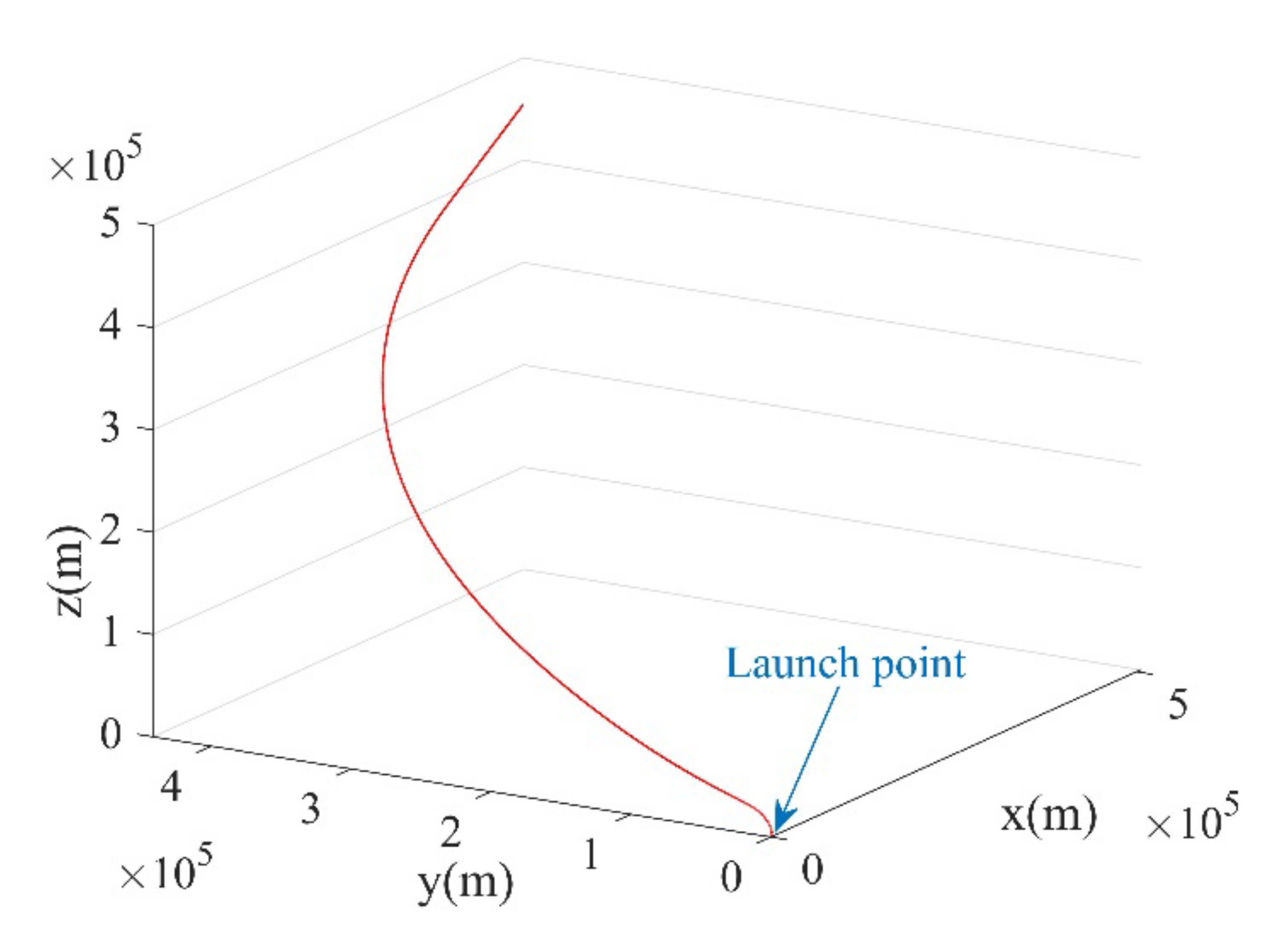
Based on the above simulation conditions, the simulated aerospace vehicle launch trajectory is shown in Figure 5.

In order to verify the performance of the robust filtering algorithm of the integrated navigation system under the launch inertial coordinate system proposed in this paper, the above simulation condition is set as base; a simulation comparison of the algorithm in this paper with the KF algorithm and the UKF algorithm is carried out. The results are shown as follows.

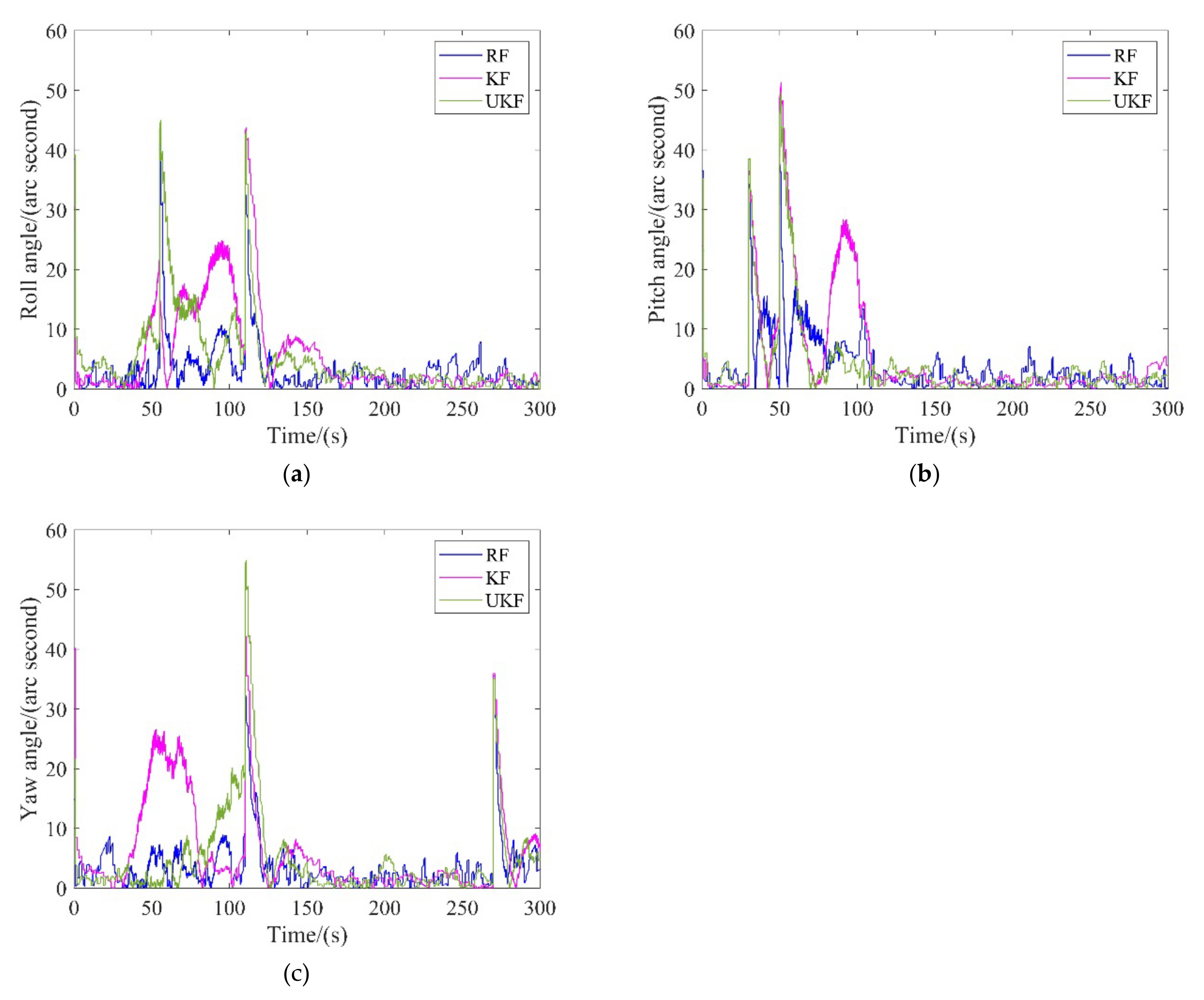
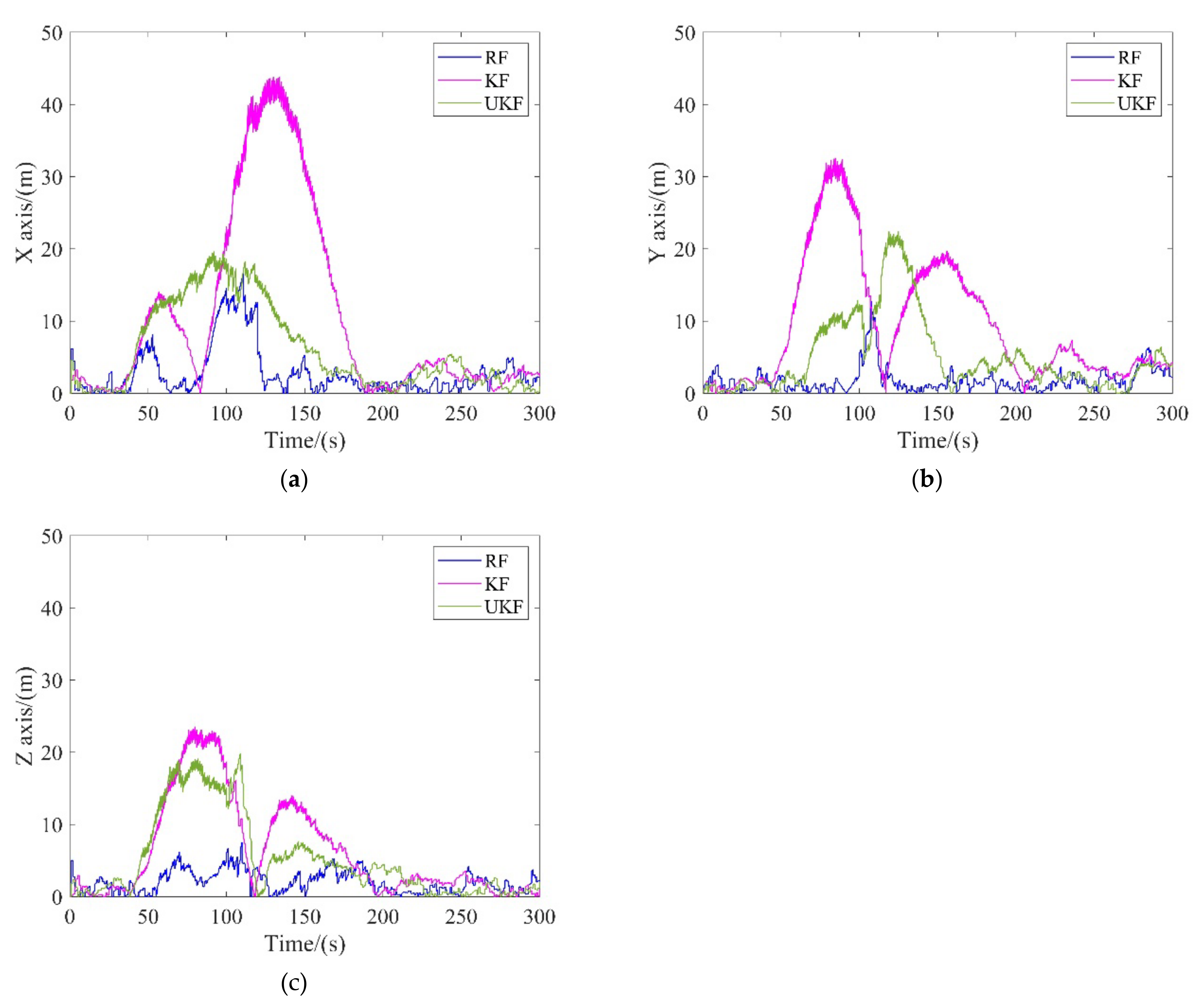
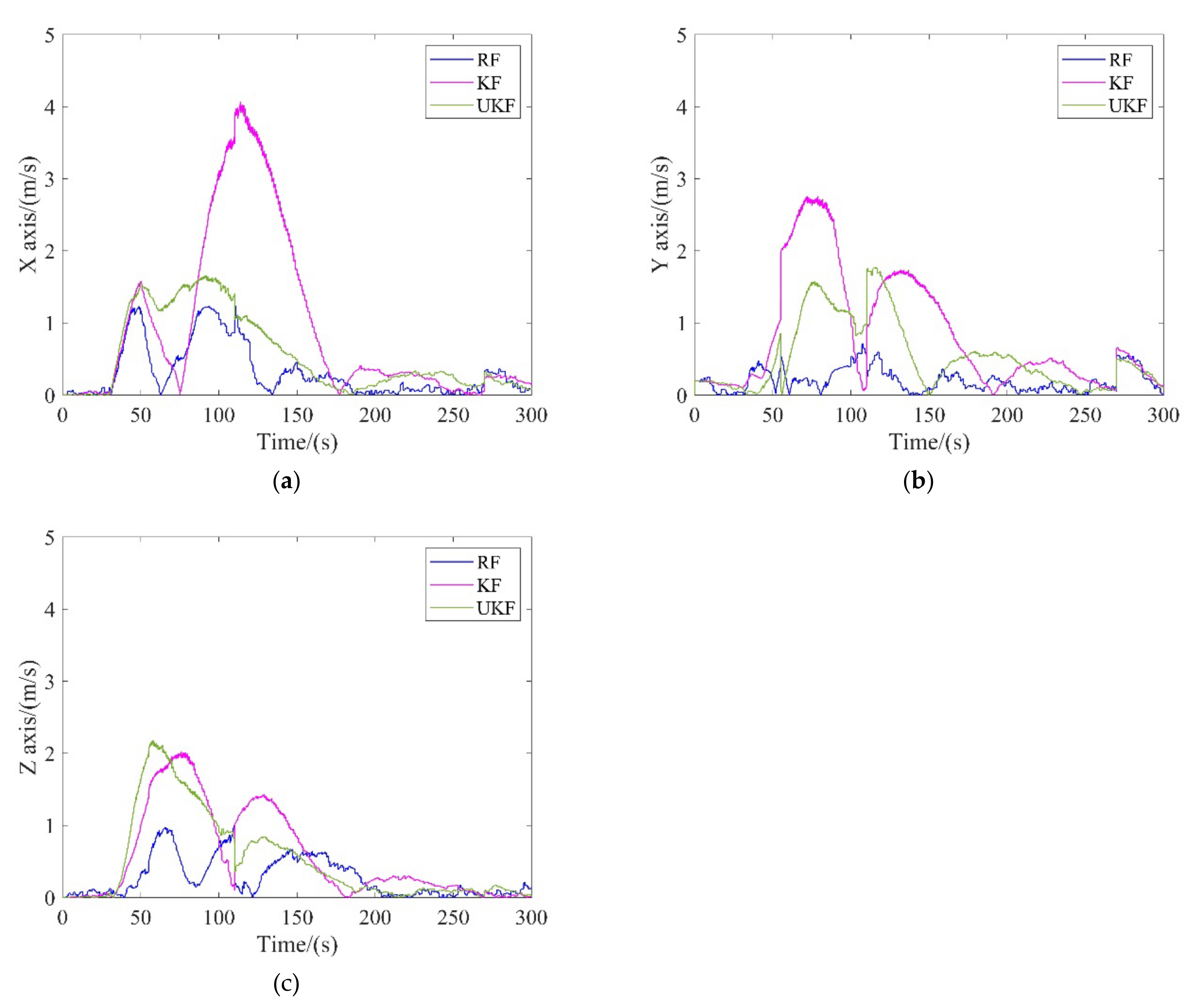
Figure 6, Figure 7 and Figure 8 are the comparison diagram of the attitude, positioning and velocity error of the SINS/GPS/CNS integrated navigation system in the launch inertial coordinate system. The attitude of the aerospace vehicle is obtained by the inertial navigation system and celestial navigation system. The position and velocity of the aerospace vehicle are obtained by the inertial navigation system and satellite navigation system. Due to the inconsistency between the system model and the filter model in the 30–90 s, around 30 s, the three algorithms have certain fluctuations. Among them, the KF algorithm cannot make a self-adaptive adjustment according to the changes of the actual system model when the system model has been preset. The error-curve fluctuation of the UKF algorithm is less than that of the KF algorithm, because it restores the real-system model as much as possible by finding a Gaussian distribution close to the real distribution. However, with the inconsistency between the system model and the filter model, it is difficult to find a suitable Gaussian distribution to describe the system model, so the algorithm error increases. The RF algorithm proposed in this paper can identify and adaptively adjust the unknown input that causes the inaccuracy of the system model, so it can restore the accurate system model to the greatest extent.

At the same time, in the simulation conditions, the navigation sensor fails in 100 s–120 s. The error curve of the KF algorithm diverges rapidly after 100 s, indicating that it cannot work normally when the navigation sensor fails. The UKF algorithm determines the optimal gain matrix according to the covariance matrix of the filter and the covariance of the measured value, and then calculates the sampling points, which are determined by the state equation and the measurement equation. Therefore, it can adapt to the sudden change of the measurement information to a certain extent, but from the experimental results, it will still diverge in the case of continuous failure of the measurement information. The RF algorithm proposed in this paper can adaptively adjust the covariance matrix of the system measurement noise by detecting the fault measurement information, and finally ensure the accuracy of the navigation system when the navigation sensor fails.

It can also be seen from

Table 3. Root mean square error data estimated by three algorithms (Condition A).

	KF	UKF	RF
Roll (″)	9.8847	8.7435	5.9599
Pitch (″)	10.5008	8.1840	6.3841
Yaw (″)	10.0725	9.0390	5.7409
X axis (m)	17.0252	8.5108	4.4062
Y axis (m)	12.6399	7.2346	2.4677
Z axis (m)	9.1462	7.7229	2.5166
X axis (m/s)	1.5030	0.7806	0.4771
Y axis (m/s)	1.1377	0.7069	0.2559
Z axis (m/s)	0.8402	0.7887	0.3756

and

Table 4. Root mean square error data estimated by three algorithms (Condition B).

	KF	UKF	RF
Roll (″)	9.8904	9.1761	6.8103
Pitch (″)	19.0265	9.6734	6.3942
Yaw (″)	10.3397	9.8092	7.1629
X axis (m)	21.9449	12.0101	5.1014
Y axis (m)	20.4995	10.2390	4.2343
Z axis (m)	22.1283	11.3863	3.6555
X axis (m/s)	1.6037	1.0580	0.7214
Y axis (m/s)	1.4885	0.9294	0.4935
Z axis (m/s)	1.5118	1.0129	0.4895

that when the system model is inconsistent with the filter model and the navigation system measurement information is invalid, the root mean square error data of the attitude, position and velocity error of the Kalman algorithm are larger than those of the UKF algorithm. In the RF algorithm used in this paper, the root mean square error of the attitude, position and velocity are significantly lower than those of Kalman algorithm and UKF algorithm, mainly because the algorithm in this paper can independently identify, estimate and compensate the unknown inputs to the equation of state. At the same time, it can realize the adaptive estimation noise variance matrix of the measurement, which makes the system better in fault tolerance and stronger in robustness.

5. Conclusions

In this paper, we analyze and study the robustness filtering algorithm for the navigation system of the aerospace vehicle. As an aircraft that can fly across the dual fields of aviation and aerospace, the aerospace vehicle is gradually being valued by various countries. As an important part of its control loop, a high-precision and robust navigation system is indispensable. However, the main problem faced by navigation systems of the aerospace vehicle is difficulty in meeting the large dynamic and multi-task working mode of the aerospace vehicle. The existing navigation algorithms can only adapt to the situation in which the navigation system model and the filter model are consistent. When the models are inconsistent, the navigation accuracy drops faster. At the same time, complex working environments such as large dynamic flight may cause the star sensor to be unable to observe the stars, etc., effectively. The navigation system must be robust and fault-tolerant. Therefore, fault detection, isolation and reconstruction of measurement information are also required.

Aiming at the above problems, a multi-layer, fault-tolerant robust filtering algorithm for the aerospace vehicle navigation system in the launch inertial coordinate system is designed in this paper. Firstly, we find that the geographic coordinate system is obviously not suitable for the reference coordinate system of aerospace vehicle navigation calculation. Because the aerospace vehicle is different from the general aircraft flying near the ground—it needs to fly back and forth between space and ground—the flight has the characteristics of large dynamics. However, the existing algorithms using the geographic coordinate system as the reference coordinate system for navigation calculation usually use the simplified earth model, and the accuracy cannot meet the requirements of the aerospace vehicle navigation system. Therefore, we have established the navigation system model under the launch inertial coordinate system suitable for aerospace vehicles. On the one hand, we improved the accuracy of the navigation system by establishing an accurate earth model. On the other hand, we combined the characteristics of the navigation sensors configured by aerospace vehicles to reduce matrix conversion and improve the accuracy of the navigation system.

At the same time, most of the existing robust filtering algorithms consider the adaptive algorithm from the measurement equation of the system, but the inaccurate model in the system state equation will also reduce the robustness of the system. Therefore, we researched two parts: system state equation unknown input self-identification, self-compensation and measurement noise variance adaptation to design a multi-layer, fault-tolerant robust filter algorithm to improve the robustness of navigation system. Firstly, the inconsistency between the navigation system model and the filter model is regarded as an unknown input in the state equation and is calculated to be identified, compensated and corrected to meet the cross-airspace flight requirements of the aerospace vehicle and improve the accuracy of the navigation system. In addition, this paper solves the problem of maintaining the navigation accuracy of the navigation system in the case of a measurement-sensor failure by performing fault detection on the measurement information and adjusting adaptively the measurement noise variance matrix, which improves the fault tolerance and robustness of the navigation system. The experimental results verify the effectiveness of the algorithm in this paper. The algorithm proposed in this paper can adapt to the actual flight environment, improve the fault tolerance as well as the robustness of the aerospace vehicle navigation system, and provide a certain foundation for further research on the aerospace vehicle.

Combined with the actual navigation requirements of aerospace vehicles, this paper establishes the basic model of the integrated navigation system in launch inertial coordinate system, which solves the problem that the original simplified earth model in the geographic coordinate system is not suitable for the aerospace vehicle navigation system. In future research, we will combine the different flight characteristics of aerospace vehicles and carry out in-depth algorithm exploration around the engineering application of aerospace vehicles, so as to further improve the accuracy and reliability of its navigation system.

References

- Succa, M.; Boscolo, I.; Drocco, A.; Malucchi, G.; Dussy, S. IXV avionics architecture: Design, qualification and mission results. Acta Astronaut. 2016, 124, 67–78. [Google Scholar] [CrossRef]
- Grantz, A. X-37B Orbital Test Vehicle and Derivatives. In Proceedings of the AIAA SPACE 2011 Conference & Exposition; AIAA SPACE Forum; American Institute of Aeronautics and Astronautics, Long Beach, CA, USA, 27–29 September 2011. [Google Scholar] [CrossRef] [Green Version]
- Gross, K.H.; Clark, M.A.; Hoffman, J.A.; Swenson, E.D.; Fifarek, A.W. Run-Time Assurance and Formal Methods Analysis Nonlinear System Applied to Nonlinear System Control. J. Aerosp. Inf. Syst. 2017, 14, 232–246. [Google Scholar] [CrossRef]
- Zhao, Y. Performance evaluation of Cubature Kalman filter in a GPS/IMU tightly-coupled navigation system. Signal Processing 2016, 119, 67–79. [Google Scholar] [CrossRef]
- Kuchynka, P.; Serrano, M.A.M.; Merz, K.; Siminski, J. Uncertainties in GPS-based operational orbit determination: A case study of the Sentinel-1 and Sentinel-2 satellites. Aeronaut. J. New Ser. 2020, 124, 888–901. [Google Scholar] [CrossRef]
- Gou, B.; Cheng, Y.M.; Ruiter, A. INS/CNS navigation system based on multi-star pseudo measurements. Aerosp. Sci. Technol. 2019, 95, 105506. [Google Scholar] [CrossRef]
- Wang, R.; Xiong, Z.; Liu, J.; Shi, L. A new tightly-coupled INS/CNS integrated navigation algorithm with weighted multi-stars observations. Proc. Inst. Mech. Eng. Part G J. Aerosp. Eng. 2015, 230, 698–712. [Google Scholar] [CrossRef]
- Xu, H.; Lian, B. Fault detection for multi source integrated navigation system using Fully Convolutional Neural Network. IET Radar Sonar Navig. 2018, 12, 774–782. [Google Scholar] [CrossRef]
- Wang, R.; Xiong, Z.; Liu, J.; Cao, Y. Resilient fusion navigation based on failure influence level evaluation. IET Radar Sonar Navig. 2019, 13, 721–729. [Google Scholar] [CrossRef]
- Cui, B.; Wei, X.; Chen, X.; Wang, A. Improved high-degree cubature Kalman filter based on resampling-free sigma-point update framework and its application for inertial navigation system-based integrated navigation. Aerosp. Sci. Technol. 2021, 117, 106905. [Google Scholar] [CrossRef]
- Gao, S.; Xue, L.; Zhong, Y.; Gu, C. Random weighting method for estimation of error characteristics in SINS/GPS/SAR integrated navigation system. Aerosp. Sci. Technol. 2015, 46, 22–29. [Google Scholar] [CrossRef]
- Bu, J.; Sun, R.; Bai, H.; Rui, X.; Fei, X.; Zhang, Y.; Ochieng, W.Y. A Novel Integrated Method for the UAV Navigation Sensor Anomaly Detection. IET Radar Sonar Navig. 2017, 11, 847–853. [Google Scholar] [CrossRef]
- Wang, L.; Cheng, X. Algorithm of gaussian sum filter based on high-order UKF for dynamic state estimation. Int. J. Control. Autom. Syst. 2015, 13, 652–661. [Google Scholar] [CrossRef]
- Urrea, C.; Rodrigo, M. Joints Position Estimation of a Redundant Scara Robot by Means of the Unscented Kalman Filter and Inertial Sensors. Asian J. Control. 2015, 18, 481–493. [Google Scholar] [CrossRef]
- Magree, D.; Johnson, E.N. Factored Extended Kalman Filter for Monocular Vision-Aided Inertial Navigation. J. Aerosp. Inf. Syst. 2016, 13, 475–490. [Google Scholar] [CrossRef]
- Wang, J.; Chen, Z. Variational Bayesian Iteration-Based Invariant Kalman Filter for Attitude Estimation on Matrix Lie Groups. Aerospace 2021, 8, 246. [Google Scholar] [CrossRef]
- Lim, J.; Shin, M.; Hwang, W. Variants of extended Kalman filtering approaches for Bayesian tracking. Int. J. Robust Nonlinear Control. 2017, 27, 319–346. [Google Scholar] [CrossRef]
- Chai, R.; Tsourdos, A.; Savvaris, A.; Chai, S.; Chen, C. Review of advanced guidance and control algorithms for space/aerospace vehicles. Prog. Aerosp. Sci. 2021, 122, 100696. [Google Scholar] [CrossRef]
- Madany, Y.M.; El-Badawy, E.; Ismail, N.; Soliman, A.M. Investigation and realisation of integrated navigation system using optimal pseudo sensor enhancement method. Radar Sonar Navig. IET 2019, 13, 839–849. [Google Scholar] [CrossRef]
- Colagrossi, A.; Lavagna, M. Fault Tolerant Attitude and Orbit Determination System for Small Satellite Platforms. Aerospace 2022, 9, 46. [Google Scholar] [CrossRef]
- Xiong, K.; Wei, C.L.; Liu, L.D. Robust multiple model adaptive estimation for spacecraft autonomous navigation. Aerosp. Sci. Technol. 2015, 42, 249–258. [Google Scholar] [CrossRef]
- Zheng, X.; Wu, H. Robust filtering algorithm against hybrid-attacks and randomly occurring nonlinearities: Application to a quadrotor UAV. Digit. Signal Processing 2021, 117, 103159. [Google Scholar] [CrossRef]
- Li, H.; Yan, L.; Xia, Y. Distributed Robust Kalman Filtering for Markov Jump Systems With Measurement Loss of Unknown Probabilities. IEEE Trans. Cybern. 2021. [Google Scholar] [CrossRef]
- Pan, C.; Li, Z.; Gao, J.; Li, F. A Variational Bayesian-Based Robust Adaptive Filtering for Precise Point Positioning Using Undifferenced and Uncombined Observations. Adv. Space Res. 2020, 67, 1859–1869. [Google Scholar] [CrossRef]
- Fu, H.; Yang, H.; Wen, X. Self-identification and self-calibration Kalman filtering method. J. Deep. Space Explor. 2019, 6, 5. [Google Scholar] [CrossRef]
- Teunissen, P.J.G. Batch and Recursive Model Validation. In Springer Handbook of Global Navigation Satellite Systems; Teunissen, P.J.G., Montenbruck, O., Eds.; Springer International Publishing: Cham, Switzerland, 2017; pp. 687–720. [Google Scholar] [CrossRef]
Figure 1.
INS/CNS/GPS integrated navigation algorithm structure diagram in launch inertial coordinate system.
Figure 2.
The conversion relationship between the launch inertial coordinate system and the J2000 inertial coordinate system.
Figure 3.
Multi-layer robust and fault-tolerant filter design structure.
Figure 4.
Flow chart of algorithm.
Figure 5.
Simulation diagram of aerospace vehicle trajectory.
Figure 6.
(a) Roll-angle error contrast curves; (b) Pitch-angle error contrast curves; (c) Yaw-angle error contrast curves. Angle-error contrast curves under the launch inertial coordinate system.
Figure 7.
(a) X-axis position error contrast curves; (b) Y-axis position error contrast curves; (c) Z-axis position error contrast curves. Position error contrast curves under the launch inertial coordinate system.
Figure 8.
(a) X-axis velocity error contrast curves; (b) Y-axis velocity error contrast curves; (c) Z-axis velocity error contrast curves. Velocity error contrast curves under the launch inertial coordinate system.