
Optimal Aggressive Constrained Trajectory Synthesis and Control for Multi-Copters


Department of Mechanical and Aerospace Engineering, The University of Texas at Arlington, 500 W. First St, Box 19018, 211 Woolf Hall, Arlington, TX 76019, USA
*
Author to whom correspondence should be addressed.
†
These authors contributed equally to this work.
Aerospace 2022, 9(6), 281; https://0-doi-org.brum.beds.ac.uk/10.3390/aerospace9060281
Submission received: 11 April 2022
/
Revised: 11 May 2022
/
Accepted: 17 May 2022
/
Published: 24 May 2022
(This article belongs to the Special Issue Applications of Drones)
Abstract
:In this paper, we propose a novel time and control effort optimal aggressive trajectory synthesis and control design methodology. The trajectory synthesis is a modified minimum snap design but with specific position and orientation constraints on a multi-copter, such as flying through tight spaces (windows) at specific orientations. The paper also introduces a means to stitch together multiple flight segments, enforce smoothness, and minimize segment times as well as the overall time, thereby resulting in very aggressive and feasible trajectories. A novel analysis for a specific scenario when no yaw angle specifications are provided is conducted, wherein a trade-off results in additional aggressiveness. The control algorithms to follow these trajectories are based on an inverse dynamics approach. Several candidate high-fidelity simulations are performed to verify the effectiveness of the proposed approach.
1. Introduction
Multi-copters, such as quadcopters, hexacopters, octocopters, and others have been very popular in recent years mainly because of their availability, mobility, agility, and flexibility. They are a great platform for control experiments and various applications. Their characteristics also make them an attractive choice for high-speed aerial navigation through complex environments. Various researches related to aggressive trajectory generation and aggressive maneuver tracking have been conducted. Some recent examples include [1], in which the authors proposed a novel control law for accurate tracking of aggressive quadcopter trajectories. In [2] the authors presented a framework to do optimal time allocation for quadcopter trajectory generation. In [3] the authors addressed the problem of performing aggressive quadcopter maneuvers that are attitude-constrained.
Our main contribution in this paper is the development of a synthesis framework that fully utilizes the available dynamic capability of the multi-copter when performing the most aggressive maneuver. We pursue aggressiveness because time is a critical issue in the given scenario. We adopt aggressive maneuvers because the environment is complicated and sometimes very specific maneuvers are needed in order to satisfy path and vehicle state constraints, given the environment model. However, the level of aggressiveness one can achieve depends on the optimality of the trajectory plan and the dynamic capability of the vehicle. It will be valuable if one can generate a trajectory that fully utilizes the dynamic capability of the vehicle while accommodating the maneuvers required at specific locations. Therefore, in this research, we assume that the dynamic capability of the multi-copter is limited by its maximum rotor thrust and define the aggressiveness accordingly.
For multi-copter trajectory generation and motion control, ideas such as multi-segment polynomial, minimum derivative optimization, and differential flatness inverse dynamics analysis are widely adopted [4,5,6]. To achieve an aggressive trajectory, methods such as segment time allocation [7] and spatial-temporal trajectory [2] have been proposed. However, we do not yet have a synthetic architecture to find the most aggressive trajectory based on the waypoints, the requirement for vehicle heading and maneuvering at waypoints, and the constraints of rotor thrust for a multi-coper. We would further like to emphasize that the contribution of this research lies in the development of a complete synthesis to fulfill this gap. The constraint on vehicle maneuvering at waypoints is posed as a window passing through problem and solved through the trajectory optimization as trajectory derivative constraints. The maximum rotor thrust for the trajectory is obtained through the inverse dynamics analysis. As the optimized aggressive trajectory is obtained, a geometric controller is used to perform the polynomial trajectory tracking and verify the feasibility of the trajectory and the accuracy of the inverse dynamics analysis. Further, a novel method for yaw trajectory optimization is also proposed to further improve the aggressive performance in the case when there are no specific requirements on the vehicle heading.
The rest of the paper is organized as follows. Section 2 describes the problem and the setup. Section 3 summarizes the mathematical modeling providing the basic governing equations. Section 4 discusses the solution methodology in detail, followed by the numerical results in Section 5. Section 6 summarizes the performance of the geometric controller with Section 7 providing details on the modification to the trajectory should there be no heading constraints. Finally, Section 8 provides concluding remarks and summarizes future work.
2. Problem Description and Setup
While aggressive flight using multi-copters is widely discussed/mentioned, there is not much effort put toward defining aggressiveness and finding the most aggressive trajectory with complex maneuver requirements for a given vehicle model. Therefore, in this paper, the problem is addressed as: Given waypoint coordinates, heading angles, and some vehicle velocity and attitude constraints at these waypoints, how can we find a feasible trajectory that fully utilizes the dynamic capability of a multi-copter to achieve the optimal aggressiveness? A formal definition of aggressiveness will be provided in the latter sections.
3. Mathematical Model Description
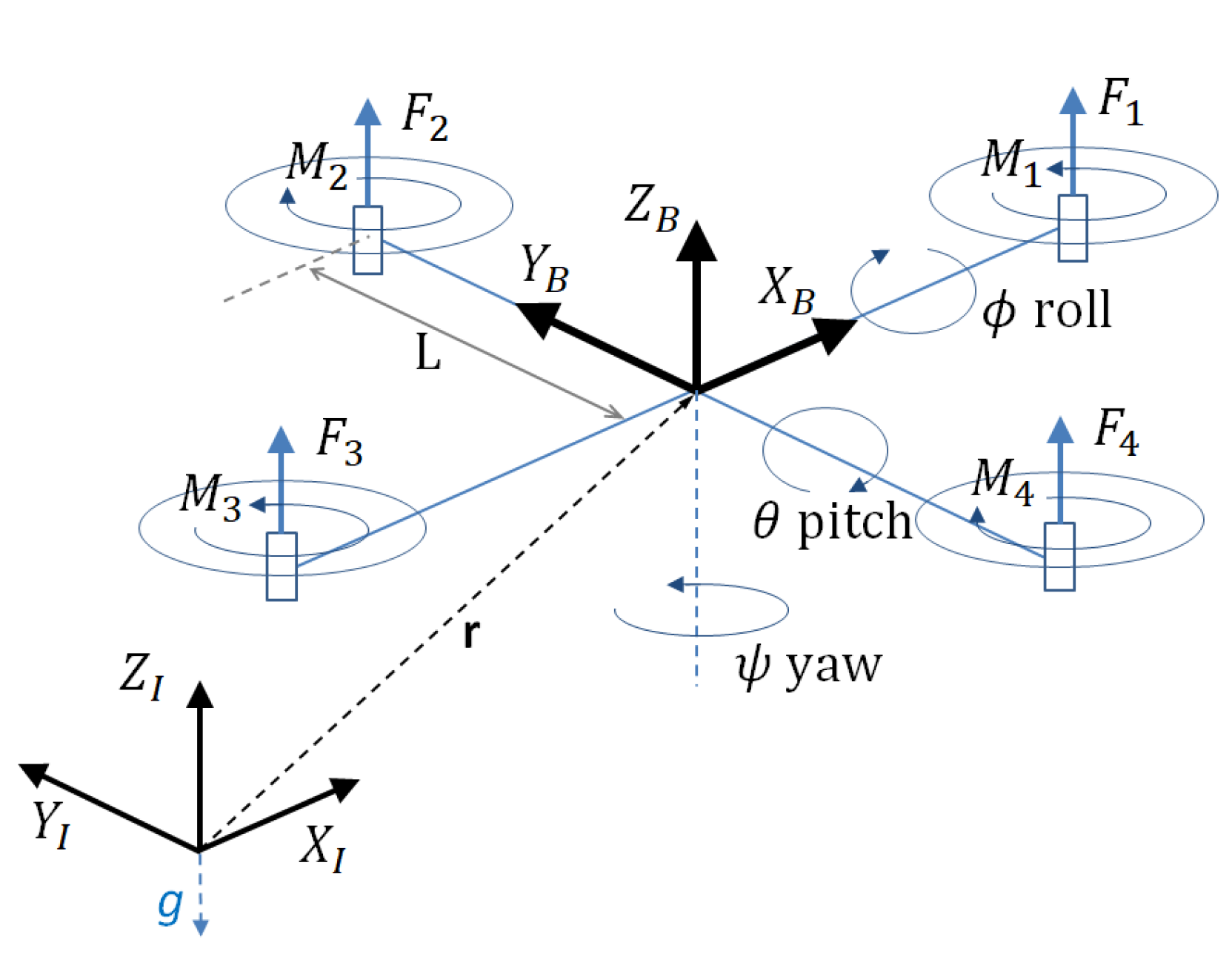
A generic model for quadcopters is used in this paper. Note that the proposed approach can be applied to different configurations of multi-copters by modifying the vehicle force and moment model according to the desired rotor configuration and control allocation method. The coordinate systems and forces and moments generated by the rotors are shown in Figure 1.
The body frame, B, is attached to the center of mass of the quadcopter and rotor 1 is on the positive -axis. The gravitational acceleration g is in the direction of the inertial frame, I. Euler angles roll , pitch , and yaw are used to define orientation from inertial frame to body frame. Note, rotation order is used here, and therefore the rotation matrix for transforming coordinates from B to I is given by:
The position vector of the quadcopter in the inertial frame is denoted by . With the gravity force acting in the direction and the forces of the rotors acting in the direction, the equation governing the acceleration of the quadcopter with respect to inertial frame is given by:
With p, q, and r denoting the components of angular velocity of the quadcopter in the body frame, the rotational kinematics equation is given by:
Assuming rotors 1 and 3 rotate in the direction while 2 and 4 rotate in the direction, and act in the direction while and act in the direction since the moment produced by the rotor is opposite to the direction of rotation of the blade. With denoting the moment of inertia of the quadcopter referenced to the center of mass and L denoting the distance from the axis of rotation of the rotors to the center of the quadcopter, the rotational dynamics equation is given by:
Define the input wherein is the total force from the rotors and , and are the moments about , and axes. Following [6], we assume that the force and moment produced by the ith rotor are proportional to the square of its rotational speed as:
The relationship between the input and the angular speed of the rotors can be represented as:
4. Solution Methodology
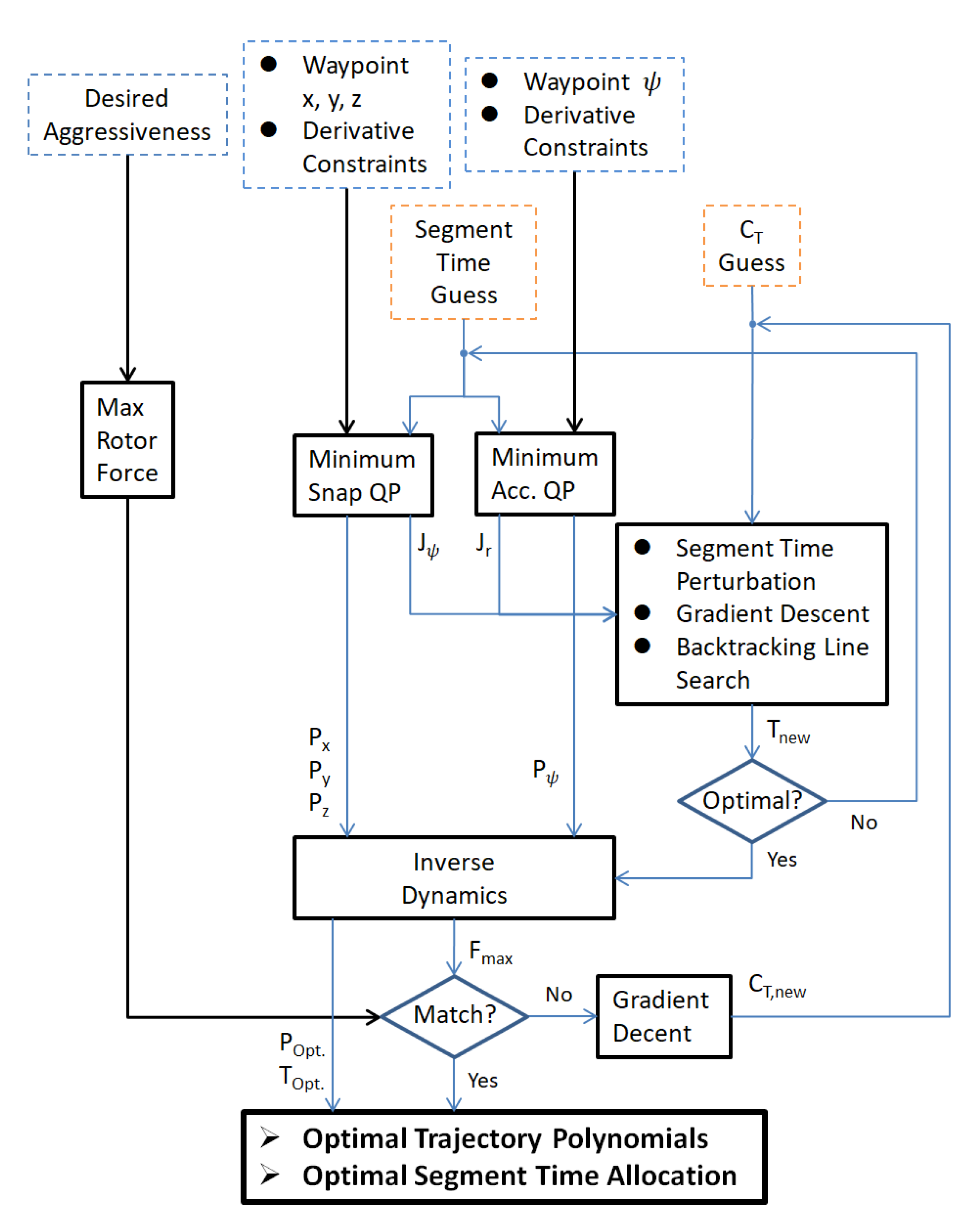
We use multi-segment polynomials to generate the trajectory and assure its smoothness by having trajectory derivative continuities. To optimize the polynomial coefficients, we form the quadratic problem with the cost on the trajectory derivative which is related to the actuator input of the vehicle. We accommodate waypoint velocity and attitude requirements in the optimization problem as equality constraints. To optimize the segment time between waypoints, we introduce an augmented cost on both trajectory derivative and total time. We connect the polynomial trajectory and actual quadcopter dynamics and rotor inputs by performing inverse dynamics analysis. We finally define aggressiveness and find the optimal trajectory with desired aggressiveness by tracking the desired maximum rotor force needed for the optimized trajectory. The whole methodology and the solution procedure are illustrated below in Figure 2.
4.1. Multi-Segment Polynomial Trajectory Optimization
Multi-segment polynomials are used to generate the trajectory. For each segment connecting one and the subsequent waypoint, independent polynomials are used to represent the quadcopter states x, y, z, and (yaw angle). Each polynomial segment is represented as:
The cost function on the integral of the quadratic of the trajectory derivatives is:
where T is the flight time for the trajectory segment and is user-specified penalty on the derivative of the trajectory. This function can be written in matrix form as:
where and is the cost matrix. Following the formulation in [4], can be constructed as:
In this paper, to minimize the input needed to achieve optimal aggressiveness, we adopted the choice in [5] which is to minimize the snap (4th derivative) in trajectory x, y, and z while minimizing the acceleration (2nd derivative) in trajectory . Therefore, we use while all other coefficients are set to zero for x, y, and z polynomial, and only for yaw polynomial. The constraints on the derivatives on the endpoints of a polynomial segment can be imposed as a linear function of the coefficients:
where is constructed by evaluating the components in the derivative formulations of the polynomial at and corresponding to the appropriate coefficients as:
We use the 0th order derivative constraint to specify the waypoint position. Higher order derivatives can be used to specify desired waypoint velocity, acceleration, etc., e.g., to enforce that the quadcopter starts from rest at the beginning of a trajectory. If not specified, these derivatives are subject to minimization of the cost function. Having assembled , , and , the quadratic problem can be written below. There are methods to solve such a standard equality constrained QP [8]. In this research, the Matlab solver “quadprog” is used.
For M polynomial segments, the joint optimization can be composed by concatenating their cost matrices in a block-diagonal fashion as:
The derivative constraints can also be concatenated in a block-diagonal fashion as:
To have a feasible smooth trajectory, the derivatives should be continuous between segments. The continuity constraints must be imposed to ensure that the derivatives at the end of the ith segment match the derivatives at the beginning of the th segment:
These constraints can be compiled into a single set of linear equality constraints for the joint optimization problem:
4.2. Constraints on Vehicle Velocity and Attitude at Waypoints
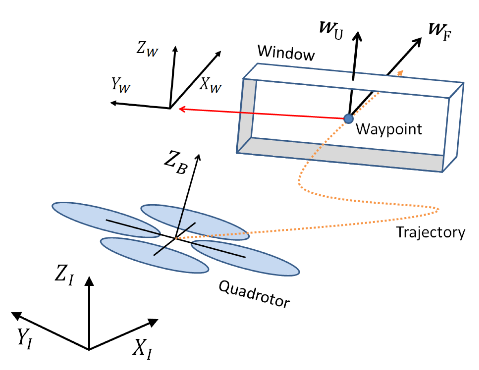
In scenarios such that the quadcopter needs to pass through some narrow gap (e.g., a window) as shown in Figure 3, we can utilize the derivative constraints to achieve the objective.
Assume a waypoint at the center of the window and the window orientation is defined with Euler angles roll , pitch , and yaw . The window forward vector in inertial frame can be obtained as:
The window upward vector in inertial frame can be obtained as:
To fly through the window safely, the velocity vector at the waypoint should be aligned with the window forward vector. Therefore, the cross product of the vectors should be zero, and the constraints for the waypoint 1st order derivatives can be composed as:
From the equation of acceleration, we can deduce that in inertial frame is in the direction of the vector :
For safely flying through the window, the vector of the quadcopter should be aligned with the window upward vector. Therefore, the constraints for the waypoint 2nd order derivatives can be composed as:
For these constraints, the relationship between x, y, and z derivatives needs to be specified. Therefore, the joint optimization of x, y, and z should be composed by concatenating their cost and constraint matrices in a block-diagonal fashion as:
where , and . With this joint optimization setup, the constraints for a window passage on waypoint s in an M-segment trajectory can be implemented as:
For a segment polynomial , the 1st order derivative (velocity) at is and . The 2nd order derivative (acceleration) at is and .
4.3. Segment Time Optimization
The above optimization finds the optimal trajectory polynomials for the given segment times. However, in general cases, we do not specify segment times, and instead, we would like to also optimize them to achieve better aggressiveness. To optimize segment times, we modify the cost function in the form:
where combines the original cost on x, y, z, and while is a penalty on total time. The cost on x, y, z is the integral of square of derivatives on distance while the cost on is on angle. To combine the costs, two coefficients and are introduced to non-dimensionalize the costs.
In this research, we minimize the 4th derivative in trajectory x, y, and z while minimizing the 2nd derivative in trajectory yaw angle. Therefore, the above equation can be represented as:
where and are defined as:
We find and in the first iteration with initial segment times and then use them as constants throughout the optimization process. With the cost function defined, we perturb each segment time by some to obtain the gradient of the cost function with respect to each segment time. This is then used in a gradient descent method to find the time allocation for the minimum cost iteratively.
Since this is a high-dimensional problem with a complex cost function, the step size can easily become too small or too large during the iterations and lead to slow convergence or even divergence. For numerical efficiency, stability, and convergence, we use the backtracking line search method [9] to find a suitable step size in every iteration.
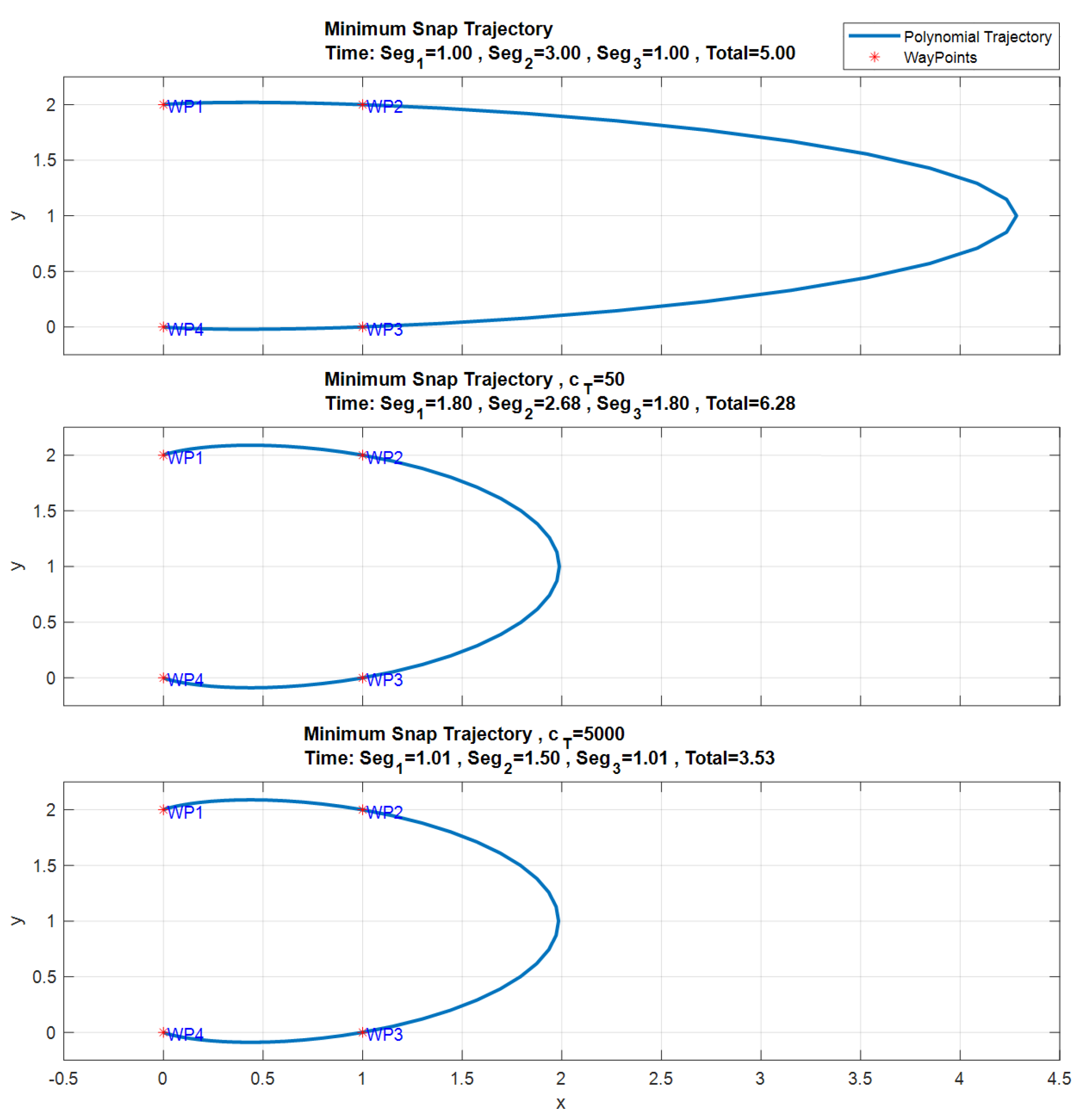
With and , we have fast and stable convergence in our test cases. Figure 4 shows the result of segment time optimization for a simple 2D 4-waypoint scenario. The initial segment time is s, and we optimize it with two different values, 50 and 5000. The result trajectories look identical because they have similar segment time distribution while the total time turned out to be 6.28 and 3.53 seconds, respectively. It is observed that, with this segment time optimization process, the optimal segment time distribution will be found to minimize the cost on integral of the square of trajectory derivatives, while the optimal total time is found based on the value of . The larger used, the smaller the total time will be, which makes the trajectory more aggressive.
4.4. Inverse Dynamics
To connect the polynomial trajectory optimization framework and actual quadcopter dynamics, we perform the inverse dynamics analysis. The differential flatness method is widely adopted in inverse dynamics analysis for multi-copters [6]. In this process, we will find all the states and inputs of the quadcopter according to the trajectory x, y, z, , and their derivatives. For orientation and , first from the equation of acceleration we have:
Assume is the vector obtained by rotating around by yaw angle :
We can determine and by:
With vehicle body frame defined, we can determine the rotation matrix and roll and pitch angles by:
For angular velocity p, q, and r, first we take the 1st derivative of the equation of acceleration:
Substituting we have:
With , the RHS is known. With , , and being unit vectors, can be considered as the projection of onto the plane with 90 shift. Therefore, the body angular velocities p and q can be determined as:
From the rotational kinematics equation, we have:
With p, q, and r solved, we have , and and can also be obtained from the inversion of the rotational kinematics equation. For angular acceleration , and , first we take the 2nd derivative of the equation of acceleration:
With , and , the RHS is known and the body angular accelerations and can be determined as:
Taking derivative of previous equation, we have:
Next we determine the moment inputs from obtained angular velocity and acceleration by the rotational dynamics equation:
Now we have found all the states and inputs of the quadcopter derived from the trajectory x, y, z, , and their derivatives. We can further determine the angular speed and force produced of each rotor by:
4.5. Max Force Tracking and Aggressiveness Defined
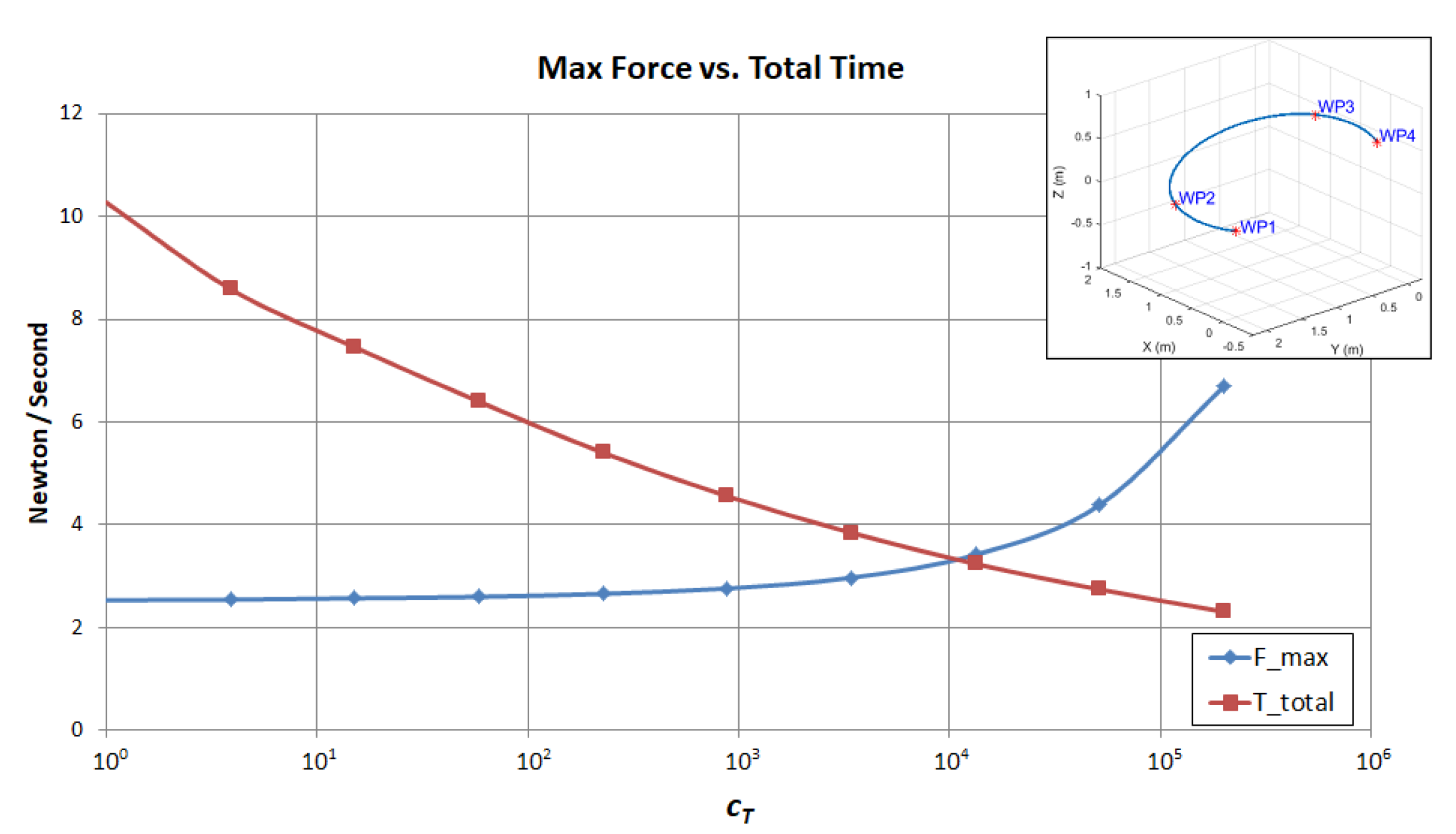
We find the maximum rotor force needed for the trajectory through the inverse dynamics analysis and observe how the maximum force and the trajectory total time vary with different values. Figure 5 shows the analysis result for a 3D 4-waypoint scenario. It is observed that, with the increment in , the total time decreases smoothly while the maximum force rises smoothly with increasing slope. With this relationship, we can track a particular total time or maximum force for a given scenario by the gradient descent method through .
With optimal aggressiveness, the quadcopter should finish the tasks in the shortest time possible by means of its dynamic capability. Generally speaking, the dynamic capability of a quadcopter is restricted by the maximum thrust of its rotors. Therefore, we define aggressiveness as the percentage of excess thrust required for the optimized trajectory.
where is the maximum rotor force required for the trajectory, is the rotor force for steady hover, and is the maximum thrust of the rotor. One might conserve the aggressiveness for safety reasons. Given waypoints x, y, z, , and the desired aggressiveness, the whole methodology to find the optimal trajectory and segment time allocation for a given quadcopter model is summarized in Figure 2.
5. Numerical Results
We test the optimization framework with a four-waypoint scenario. The waypoint settings are tabulated below (yaw angles at waypoints 2 and 3 are not specified) in Table 2.
We specify the mission to be from rest to rest, therefore the velocity and acceleration at the first and the last waypoint are constrained to be zero. There are two narrow windows to pass through in this scenario. The window settings are tabulated below in Table 3.
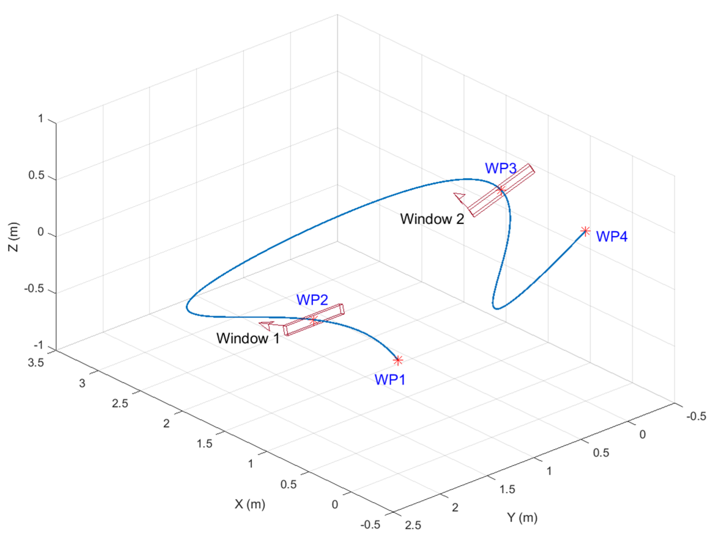
We specify the aggressiveness to be 80%. For this quadcopter model the rotor force for steady hover is N. Assuming N, we have the maximum rotor force we can use for the trajectory as N. With initial guess of s and , we use 10th order segment polynomials and have derivative continuity constraints on up to 6th order derivative (Pop). Figure 6 shows the scenario and the optimal trajectory.
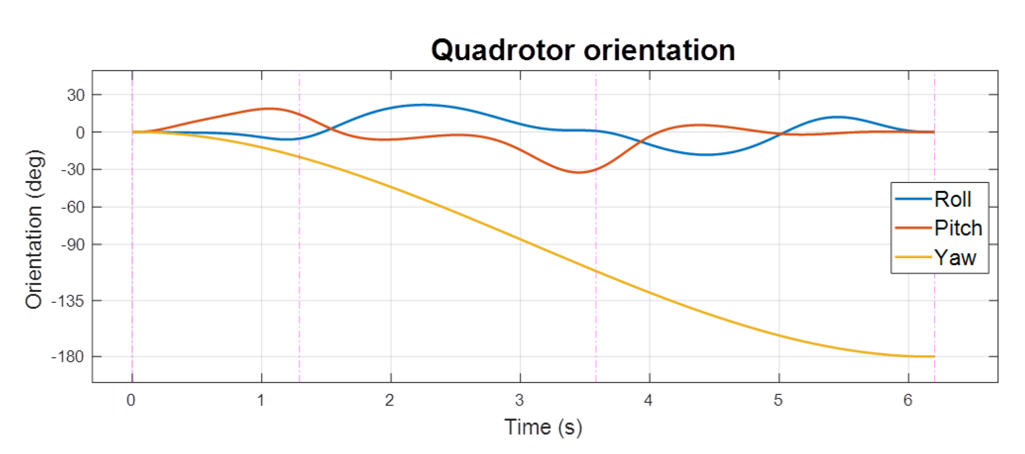
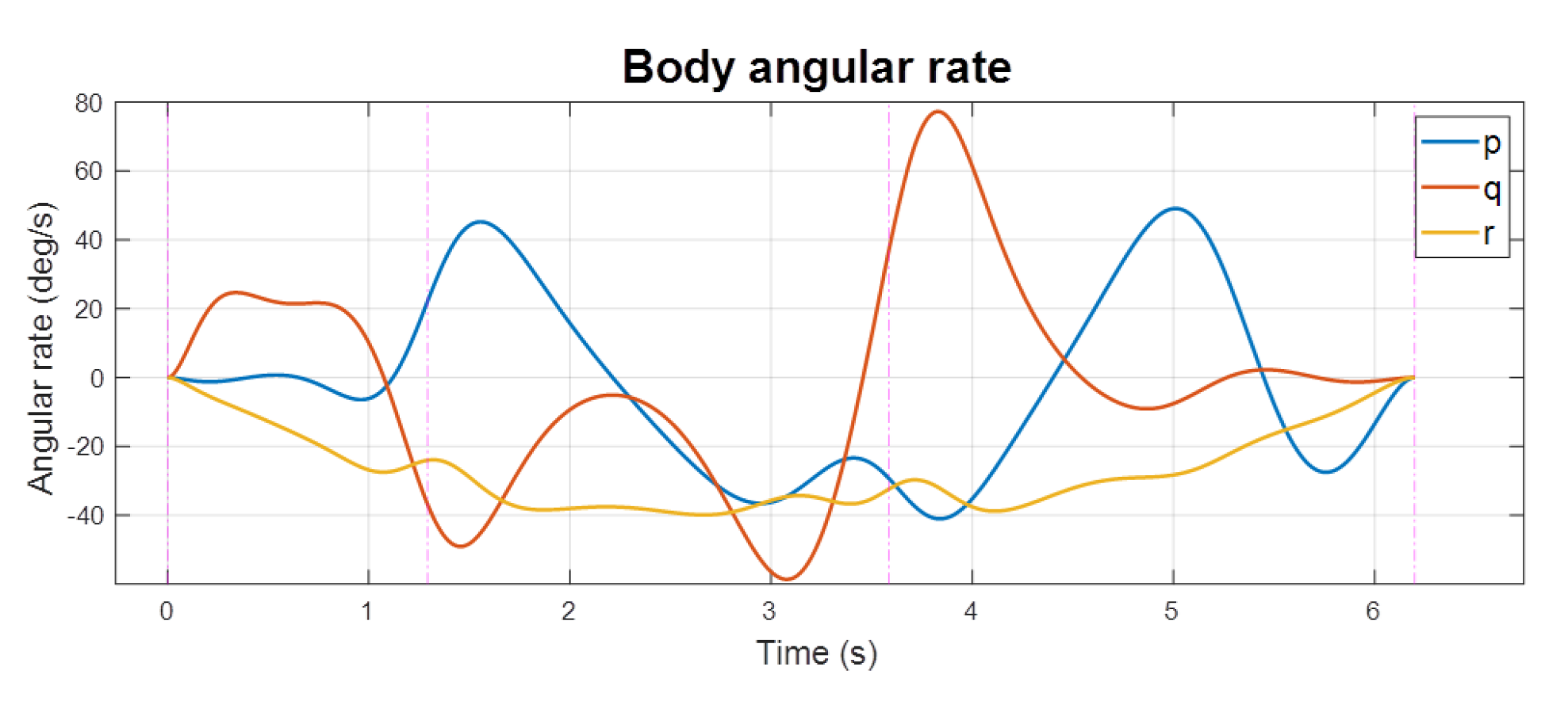
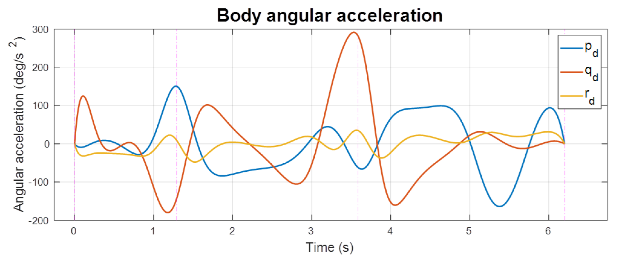
Figure 7, Figure 8 and Figure 9 show the result of the inverse dynamics analysis from the trajectory with respect to the particular quadcopter model. The magenta dashed lines mark the times of waypoint passages. It can be noticed that the quadcopter had a spike in angular acceleration and angular rate around waypoint 3 because it was making the maneuver to pass through the highly tilted window 2.
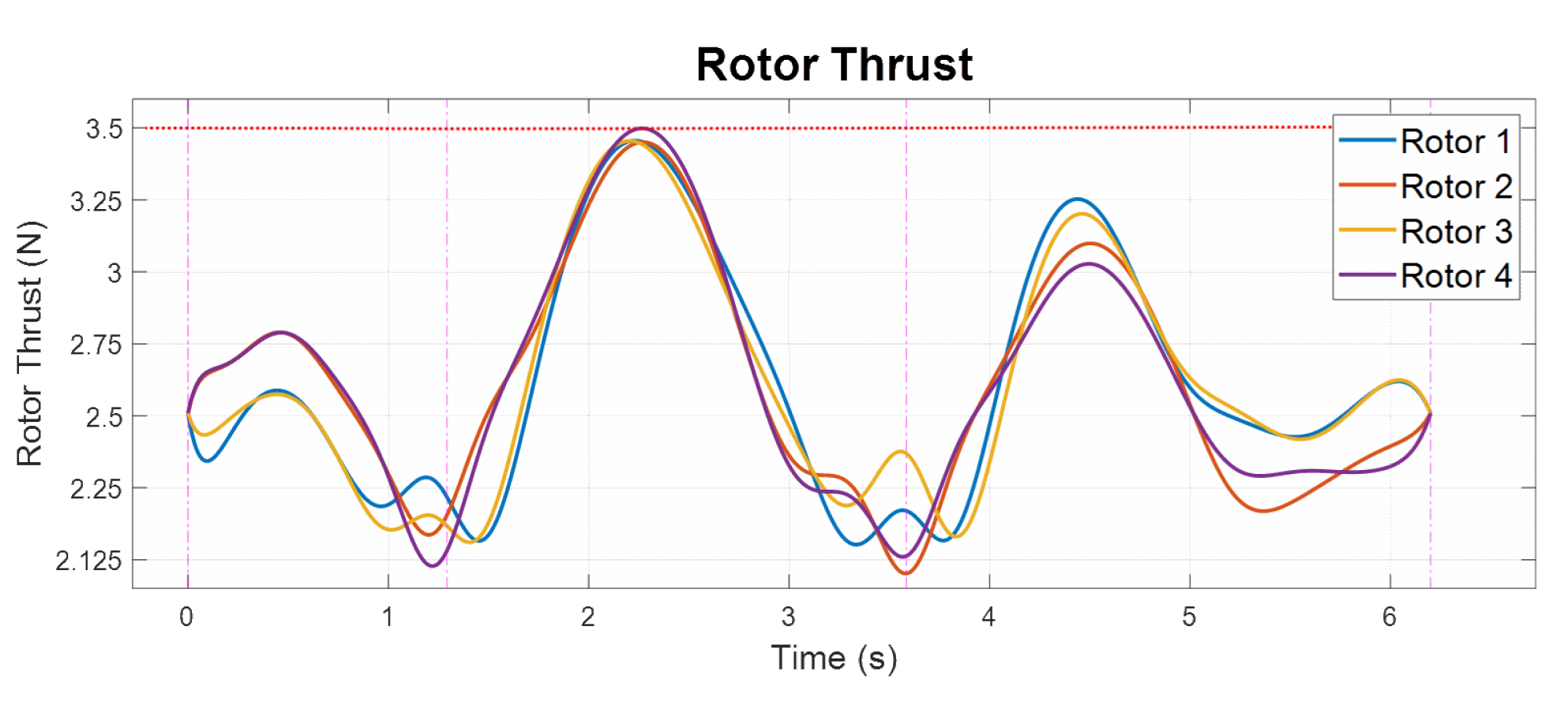
Figure 10 and Figure 11 show the control input and the rotor thrust along the trajectory. From the plot, we confirmed that the maximum rotor thrust used is N as expected.
Figure 12 shows the quadcopter on the trajectory with a fixed time interval of 0.33 s. It can be observed that the quadcopter had the highest speed in segment 2 so it can maneuver through the highly tilted window 2. The successful passage through the narrow windows can be visually confirmed. If we further check the data at waypoint 3, we have the window forward and upward vectors as and . Additionally, the quadcopter velocity and thrust vectors (aligned with ) are and . The velocity and thrust vectors are confirmed to be aligned with the window forward and upward vectors. Finally, the optimal time allocation was found as s.
6. Geometric Control and Simulation Result
To perform the polynomial trajectory tracking and verify the result of the aggressive trajectory optimization, we adopted the geometric controller proposed by Lee et al. in [11] and implemented it in MATLAB/Simulink. The controller is constructed in two parts, trajectory tracking and attitude tracking. The control input of total force f is obtained by the trajectory tracking part with:
The control input of the moments is obtained by the attitude tracking part with:
where vector defines the direction of gravity and is the rotation matrix from body to inertial frame. The tracking errors for position , velocity , attitude , and angular velocity are defined as:
where the is defined by the condition that for all . Additionally, the is the inverse of the hat map. At a given moment, , , , and represent the position, linear velocity, body angular velocity, and rotation matrix of the vehicle. The corresponding desired position and velocity are captured from the polynomial trajectory. The desired body z axis can be obtained as:
With the desired body z axis, yaw angle, and derivatives of the polynomial trajectory available, we can find the desired rotation matrix , angular velocity , and angular acceleration by following the process discussed previously in inverse dynamics. The simulation is implemented with the following equations of motion:
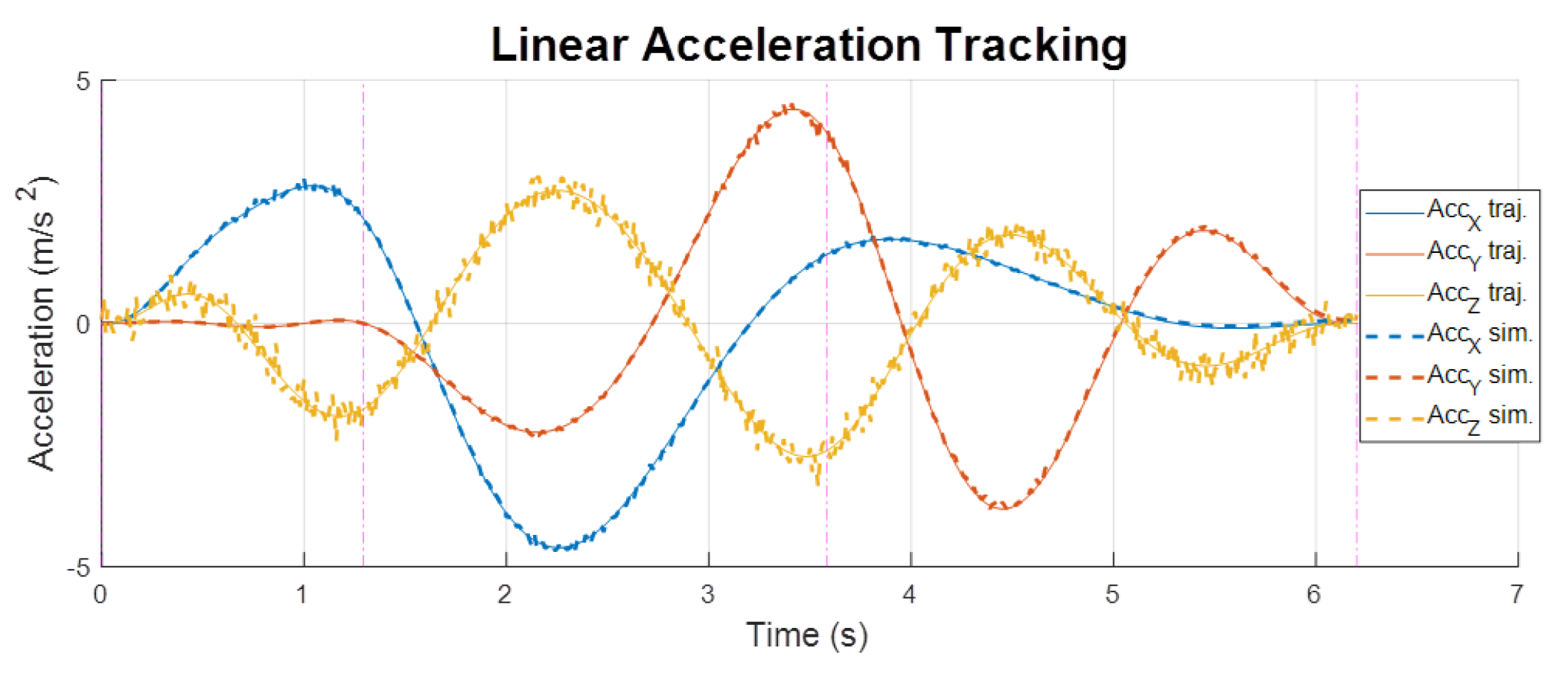
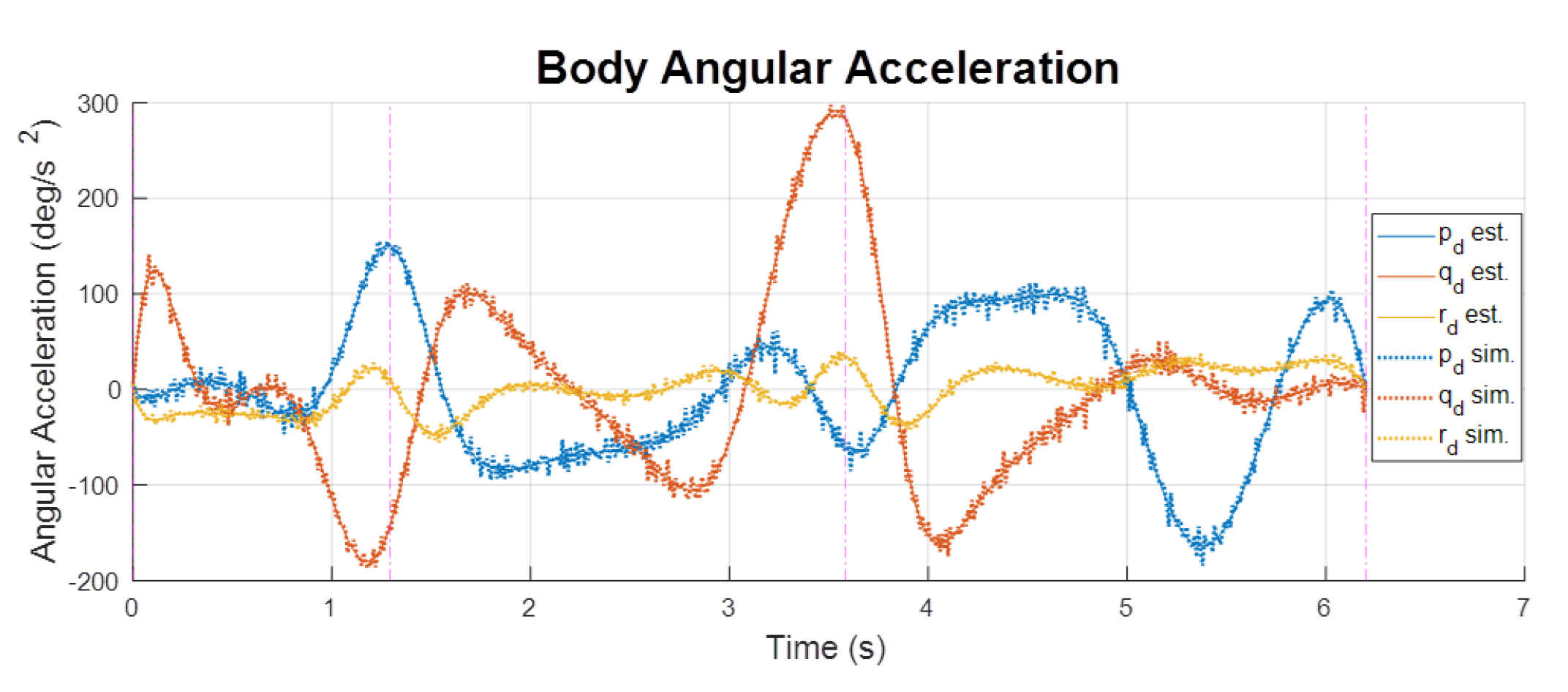
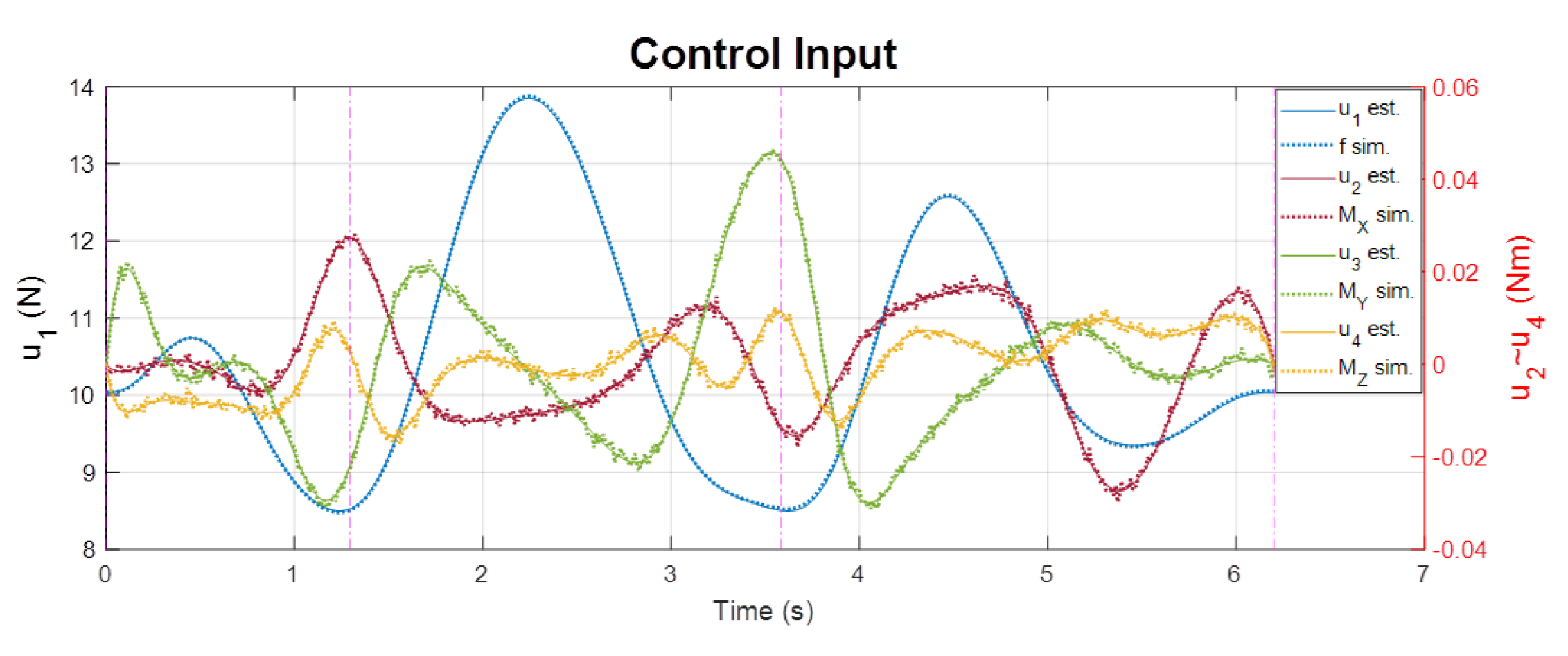
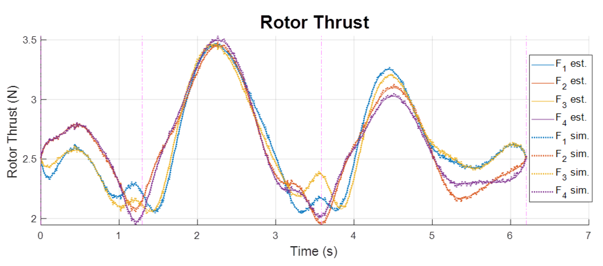
With error in estimated inertia, N noise added to f and Nm noise added to M (around of the maximum input used) as control input disturbance, we have the simulation result shown in figures below.
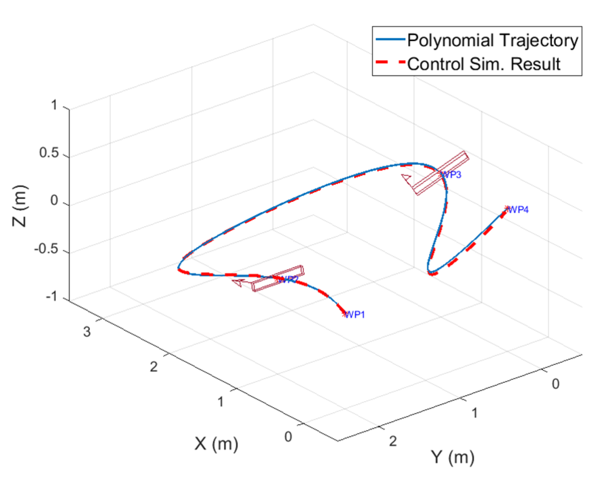
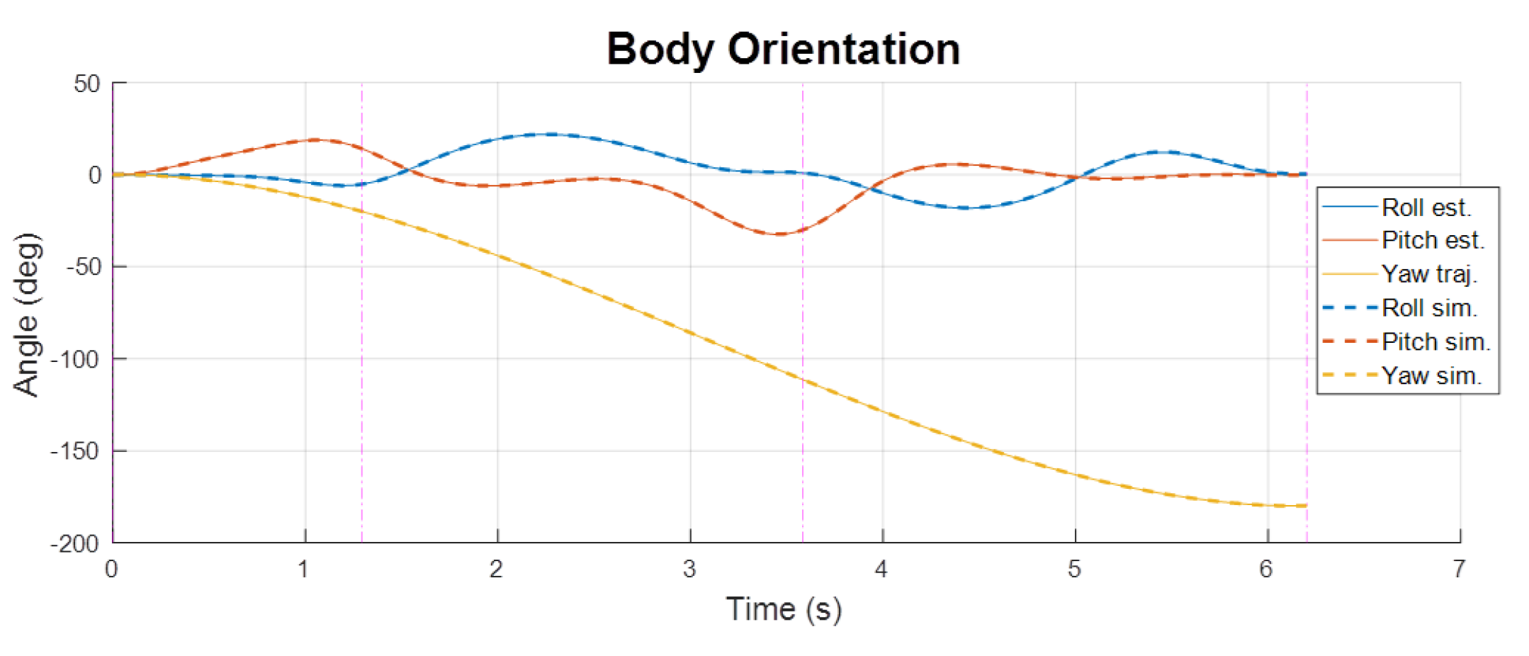
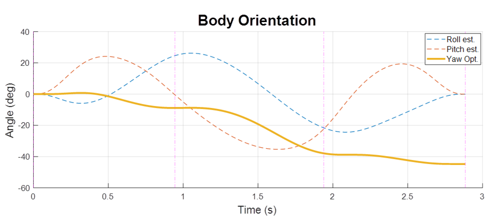
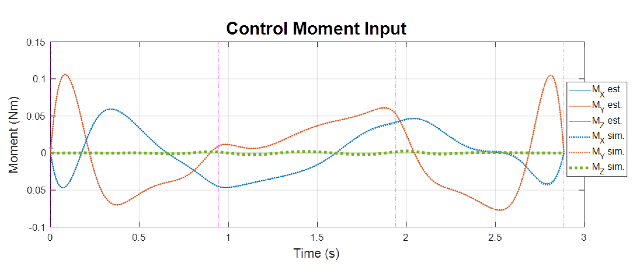
From the simulation result we can see that, despite the existence of inertia estimation error and control input disturbance, the geometric control had a good performance in tracking the polynomial trajectory. Position and yaw angle are well tracked and roll and pitch angles turned out to be very close to the inverse dynamics estimation as shown in Figure 13 and Figure 14. Therefore, the successful passage through the narrow windows is confirmed. Figure 15 and Figure 16 show that the linear acceleration is well tracked and the angular acceleration is very close to the estimation. From Figure 17, the control input used to track this polynomial trajectory is verified to be very close to the inverse dynamics estimation. The maximum rotor thrust used in the simulation is also confirmed to be around the maximum rotor force (3.5 N) requirement we specified in the trajectory generation as shown in Figure 18.
7. Yaw Trajectory Optimization
If we do not have a specific requirement on yaw angle, can we optimize the yaw trajectory to achieve better aggressive performance? In other words, by finding the yaw trajectory such that no control moment input is required to track the aggressive polynomial trajectory, we can further reduce the maximum rotor force needed and thereby track the aggressive trajectory with less motor force or achieve a faster trajectory with the same aggressiveness specified. From the equations of motion:
Because of the symmetry, the moment of inertia of the quadcopter is assumed as:
Therefore, to make , we need . Assuming the initial state , this means for the whole trajectory. Based on this, we can modify the inverse dynamics analysis to solve for and as:
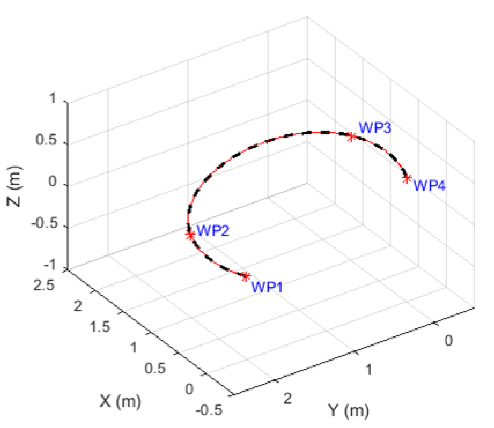
Having and at each moment in the trajectory, we can integrate iteratively throughout the inverse dynamics analysis by . Figure 19 and Figure 20 show a simple four-waypoint aggressive trajectory and the corresponding optimal yaw trajectory obtained by this method.
We converted this optimal yaw trajectory into a polynomial form and used the geometric controller to track this aggressive polynomial trajectory. Figure 21 shows that, by tracking this optimal yaw trajectory, the control input will be indeed close to zero.
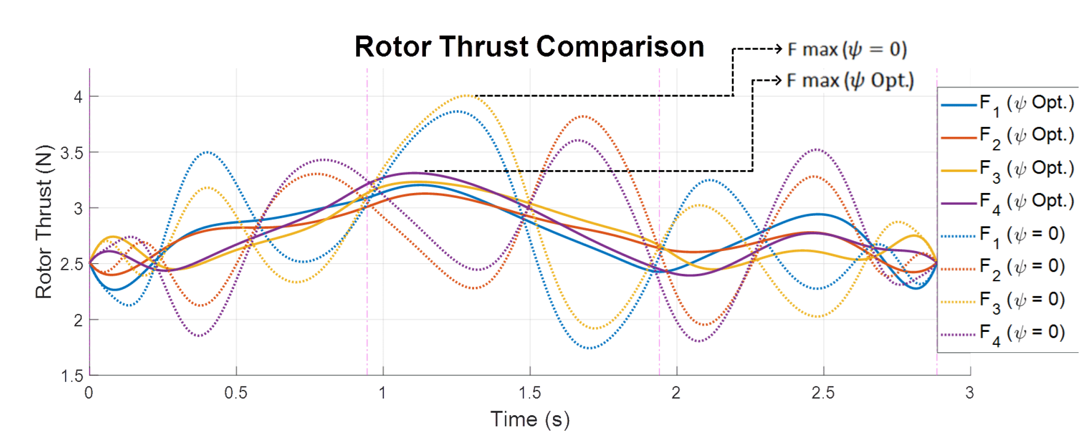
Figure 22 shows the comparison of rotor thrust used to track the aggressive trajectory between constant zero yaw and the optimal yaw trajectory. The additional yaw control effort in the constant zero yaw case pulls the and rotor forces away from the and rotor forces and thereby increases the maximum rotor force needed. From the result, we can see that, by tracking the optimal yaw trajectory, the maximum rotor force is reduced significantly by 17.5% (from 4 N to 3.3 N).
Remark 1.
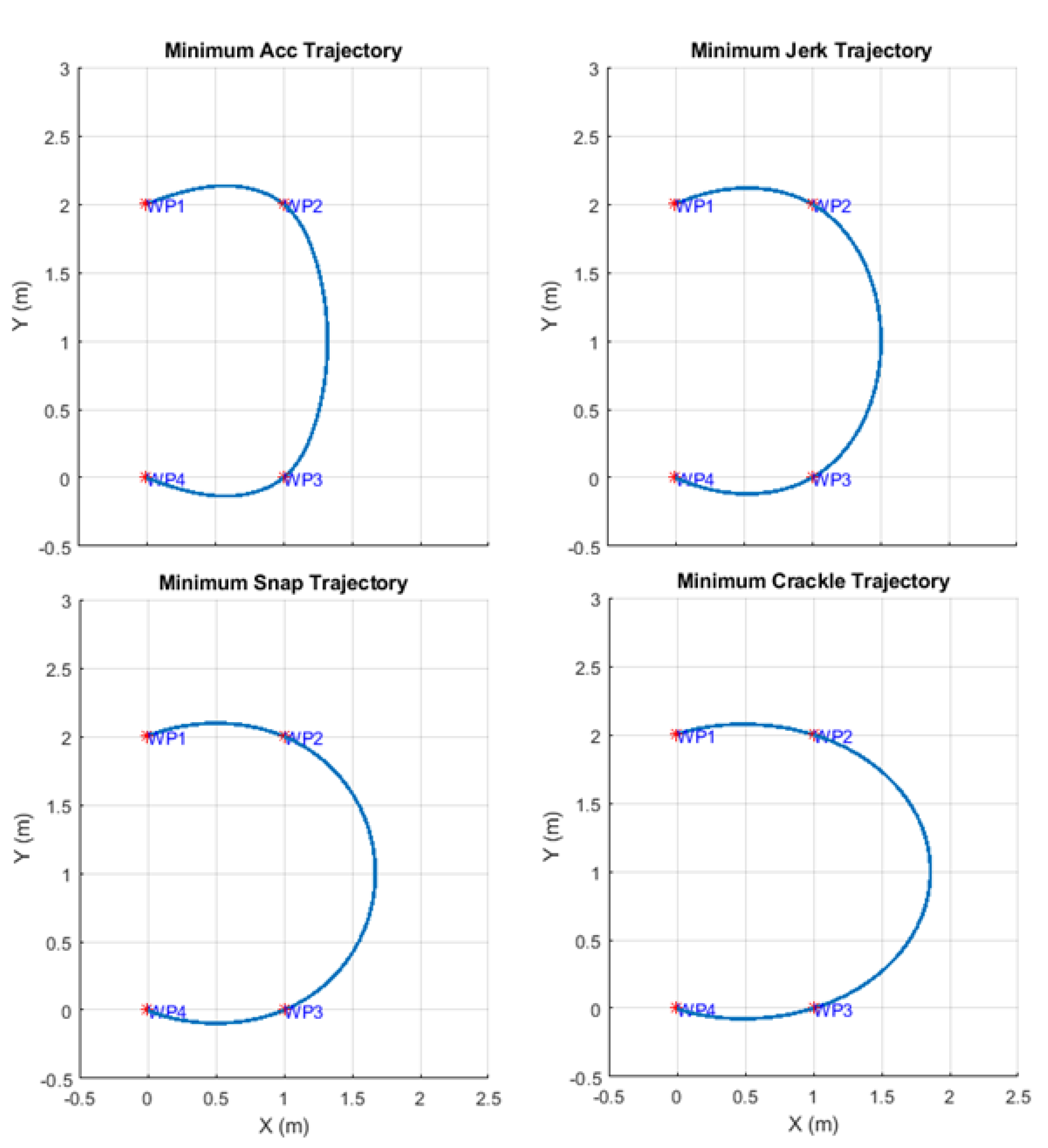
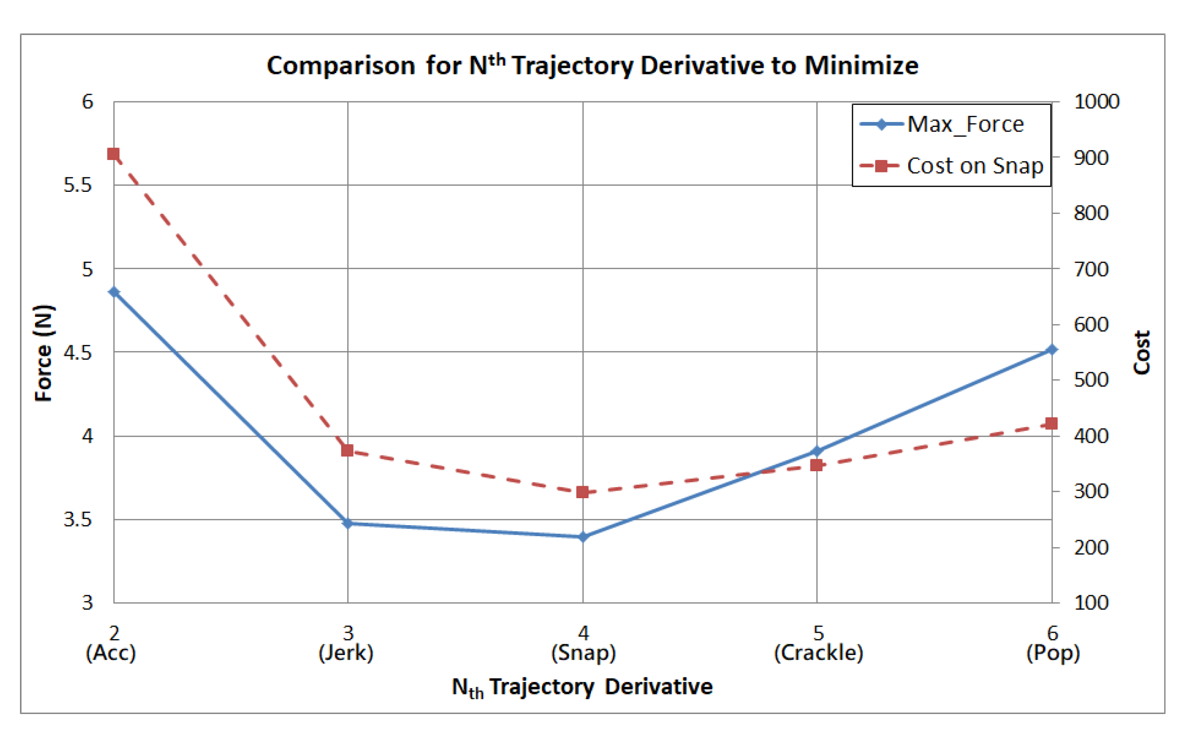
With the optimization and analysis framework developed, we review the choice of minimum snap trajectory. For the same four-waypoint scenario and segment times, we compare the optimal trajectory and the maximum rotor force required with the cost of different orders of trajectory derivatives to minimize. Figure 23 shows the geometry of the trajectories. As shown in Figure 24, the trajectory that minimizes the cost on the fourth derivative has the minimum force required. Therefore, we conclude that minimum snap is indeed the optimal choice for this approach of multi-copter aggressive trajectory optimization.
8. Conclusions
With the framework developed in this research, we can find the optimal polynomial trajectory and the corresponding segment time allocation for a given quadcopter model, a specified scenario, and a desired aggressiveness. We can also tell if the given scenario is beyond the capability of the given quadcopter by examining whether the solution exists. Furthermore, we can use the algorithm to evaluate the minimum required rotor thrust to achieve the scenario. Instead of tracking the maximum force, we can also use the algorithm to track the total time. That is, given a desired flight time, we can find the optimal trajectory that has the minimum required rotor thrust. Though the quadcopter model is used in this paper, the inverse dynamics analysis for control input (collective force and three-axis moment) applies to generic multi-copters. Therefore, the method developed in this research can be applied to multi-copters with minor modifications to the vehicle control allocation model. The geometric controller used in this research showed the capability of tracking the optimized aggressive trajectory. The tracking result verified the feasibility of the optimized trajectory and the credibility of the inverse dynamics analysis. In addition, the yaw trajectory optimization method is capable of improving the aggressive performance in the case of no requirement on heading angle.
Author Contributions
Both K.S. and T.-L.L. were involved in the conceptualization and development of methodology. T.-L.L. performed the simulations and wrote the article. K.S. reviewed and edited the manuscript for publication. All analyses were jointly performed by T.-L.L. and K.S. All authors have read and agreed to the published version of the manuscript.
Funding
This research was funded by the Office of Naval Research under grant number N00014-18-1-2215 and The National Science Foundation (S&AS) under grant number 1724248. The APC was funded by Kamesh Subbarao.
Institutional Review Board Statement
Not applicable.
Informed Consent Statement
Not applicable.
Data Availability Statement
Not applicable.
Acknowledgments
The authors acknowledge the support from the Office of Naval Research under grant number N00014-18-1-2215 and the National Science Foundation (S&AS) under grant number 1724248.
Conflicts of Interest
The authors declare no conflict of interest.
References
- Tal, E.; Karaman, S. Accurate Tracking of Aggressive Quadrotor Trajectories Using Incremental Nonlinear Dynamic Inversion and Differential Flatness. IEEE Trans. Control. Syst. Technol. 2020, 29, 1203–1218. [Google Scholar] [CrossRef]
- Gao, F.; Wu, W.; Pan, J.; Zhou, B.; Shen, S. Optimal Time Allocation for Quadrotor Trajectory Generation. In Proceedings of the IEEE/RSJ International Conference on Intelligent Robots and Systems, Madrid, Spain, 1–5 October 2018. [Google Scholar]
- Yu, G.; Cabecinhas, D.; Cunha, R.; Silvestre, C. Quadrotor trajectory generation and tracking for aggressive maneuvers with attitude constraints. IFAC-PapersOnLine 2019, 52, 55–60. [Google Scholar] [CrossRef]
- Richter, C.; Bry, A.; Roy, N. Polynomial Trajectory Planning for Quadrotor Flight. In Proceedings of the International Conference on Robotics and Automation, Karlsruhe, Germany, 6–10 May 2013. [Google Scholar]
- Mellinger, D.; Kumar, V. Minimum snap trajectory generation and control for quadrotors. In Proceedings of the International Conference on Robotics and Automation, Shanghai, China, 9–13 May 2011. [Google Scholar]
- Mellinger, D.W. Trajectory Generation and Control for Quadrotors. Publicly Access. Penn Diss. 2012, 547, 5–9. [Google Scholar]
- Richter, C.; Bry, A.; Roy, N. Polynomial Trajectory Planning for Aggressive Quadrotor Flight in Dense Indoor Environments. In Robotics Research; Inaba, M., Corke, P., Eds.; Springer International Publishing: Cham, Switzerland, 2016; pp. 649–666. [Google Scholar]
- Bertsekas, D.P. Nonlinear Programming; Athena Scientific: Belmont, MA, USA, 1999. [Google Scholar]
- Boyd, S.; Vandenberghe, L. Convex Optimization; Cambridge University Press: Cambridge, MA, USA, 2004. [Google Scholar]
- Quan, Q. Introduction to Multicopter Design and Control; Springer: Singapore, 2017. [Google Scholar]
- Lee, T.; Leok, M.; McClamroch, N. Geometric tracking control of a quadrotor uav on SE(3). In Proceedings of the 49th IEEE Conference on Decision and Control, Atlanta, GA, USA, 15–17 December 2010. [Google Scholar]
Figure 1.
Reference frames and quadcopter forces/moments.

Figure 2.
Methodology of the aggressive trajectory optimization.

Figure 3.
Relevant frames for quadcopter and window constrains.

Figure 4.
Comparison of trajectories optimized with different .

Figure 5.
Comparison of maximum rotor force and total time for trajectories optimized with different .
Figure 5.
Comparison of maximum rotor force and total time for trajectories optimized with different .

Figure 6.
Plot of the test scenario and the optimal trajectory.

Figure 7.
Vehicle Euler angles along the trajectory flight.

Figure 8.
Vehicle body angular rate along the trajectory flight.

Figure 9.
Vehicle body angular acceleration along the trajectory flight.

Figure 10.
Control input along the trajectory flight.

Figure 11.
Rotor thrust along the trajectory flight.

Figure 12.
Plot of the quadcopter along the trajectory flight.

Figure 13.
Trajectory tracking result.

Figure 14.
Vehicle Euler angle comparison.

Figure 15.
Vehicle linear acceleration tracking.

Figure 16.
Vehicle angular acceleration comparison.

Figure 17.
Control input comparison.

Figure 18.
Rotor force comparison.

Figure 19.
Simple 4-waypoint aggressive trajectory.

Figure 20.
Optimal yaw trajectory for the trajectory.

Figure 21.
Simulation result of control input with geometric controller.

Figure 22.
Rotor force comparison.

Figure 23.
Comparison of trajectories optimized with cost on different order of derivative.

Figure 24.
Maximum rotor force required for trajectories optimized with cost on different order of derivative.
Figure 24.
Maximum rotor force required for trajectories optimized with cost on different order of derivative.


Table 1.
Quadcopter parameters.
| m | 1.023 kg | g | |
|---|---|---|---|
| L | 0.2223 m | ||
Table 2.
Waypoint settings in the scenario.
| WPT Setting | ||||
|---|---|---|---|---|
| Waypoint 1 | 0 | 2 | 0 | 0 |
| Waypoint 2 | 1 | 2 | 0 | - |
| Waypoint 3 | 1 | 0 | 0.5 | - |
| Waypoint 4 | 0 | 0 | 0.5 |
Table 3.
Window (WDW) settings in the scenario.
| WDW Setting | Location | |||
|---|---|---|---|---|
| Window 1 | Waypoint 2 | |||
| Window 2 | Waypoint 3 |
Publisher’s Note: MDPI stays neutral with regard to jurisdictional claims in published maps and institutional affiliations. |
© 2022 by the authors. Licensee MDPI, Basel, Switzerland. This article is an open access article distributed under the terms and conditions of the Creative Commons Attribution (CC BY) license (https://creativecommons.org/licenses/by/4.0/).
Share and Cite
MDPI and ACS Style
Liu, T.-L.; Subbarao, K. Optimal Aggressive Constrained Trajectory Synthesis and Control for Multi-Copters. Aerospace 2022, 9, 281. https://0-doi-org.brum.beds.ac.uk/10.3390/aerospace9060281
AMA Style
Liu T-L, Subbarao K. Optimal Aggressive Constrained Trajectory Synthesis and Control for Multi-Copters. Aerospace. 2022; 9(6):281. https://0-doi-org.brum.beds.ac.uk/10.3390/aerospace9060281
Chicago/Turabian StyleLiu, Tsung-Liang, and Kamesh Subbarao. 2022. "Optimal Aggressive Constrained Trajectory Synthesis and Control for Multi-Copters" Aerospace 9, no. 6: 281. https://0-doi-org.brum.beds.ac.uk/10.3390/aerospace9060281
Note that from the first issue of 2016, this journal uses article numbers instead of page numbers. See further details here.