Article

Convergence Bounds for Limited Processor Sharing Queue with Impatience for Analyzing Non-Stationary File Transfer in Wireless Network

1
Applied Probability and Informatics Department, Peoples’ Friendship University of Russia (RUDN University), 6 Miklukho-Maklaya St., 117198 Moscow, Russia
2
Institute of Informatics Problems, Federal Research Center “Computer Sciences and Control” of the Russian Academy of Sciences, 44-2 Vavilova St., 119333 Moscow, Russia
3
Department of Applied Mathematics, Vologda State University, Lenina 15, 160000 Vologda, Russia
*
Author to whom correspondence should be addressed.
Submission received: 17 November 2021 / Revised: 13 December 2021 / Accepted: 17 December 2021 / Published: 22 December 2021
(This article belongs to the Special Issue Stability Problems for Stochastic Models: Theory and Applications II)

Abstract

:
The data transmission in wireless networks is usually analyzed under the assumption of non-stationary rates. Nevertheless, they strictly depend on the time of day, that is, the intensity of arrival and daily workload profiles confirm this fact. In this article, we consider the process of downloading a file within a single network segment and unsteady speeds—for arrivals, file sizes, and losses due to impatience. To simulate the scenario, a queuing system with elastic traffic with non-stationary intensity is used. Formulas are given for the main characteristics of the model: the probability of blocking a new user, the average number of users in service, and the queue. A method for calculating the boundaries of convergence of the model is proposed, which is based on the logarithmic norm of linear operators. The boundaries of the rate of convergence of the main limiting characteristics of the queue length process were also established. For clarity of the influence of the parameters, a numerical analysis was carried out and presented.

1. Introduction

The fifth generation (5G) networks will consist of different services with different specifications. Experts have identified network slicing as a key technology to enable 5G networks [1,2,3,4]. Within the framework of network slicing, many models are proposed with different principles for slicing radio resources [5]. In some cases, it is necessary to distribute slices between several users, and this distribution and the slices can be changed depending on time, for example, in [6,7,8], various options for re-slicing the network are shown. Earlier, we studied models for studying network slicing in the framework of papers [9,10], but we considered a model in the form of a queuing system with stationary intensities.
Given the need to re-slice the network and because all processes are non-stationary and depend on time. For example, a traffic profile—user activity is different depending on the time of day. Activity may also depend on the time of year; in the summer many users go on vacation and fly to other countries, and in winter most users are actively working and on weekends they sit at home watching movies, for example. Taking into account this dependence, it is necessary to consider models with non-stationary intensities. In our work, we consider an example of downloading user files depending on the time of day. For convenience, we consider one slice of the radio frequency channel taking into account the non-stationary nature, and look at the behavior of the characteristics. As a mathematical model, we take a queuing system with a non-stationary arrival intensity of user arrival in the system, as in [11,12], where such systems with non-stationary intensities are used for the joint service of radio frequencies.
This article discusses a special, but rather non-standard, heterogeneous birth and death process, for which, in principle, one can apply the methods described, for example, in articles [13,14], but due to the specifics of the model, in order to obtain acceptable estimates, the authors had to “trick”. In particular, the rate of convergence in the example under consideration actually turns out to be rather slow, so that the existing (and constructed) limiting regime begins to adequately show the situation at sufficiently large times Usually, uniformization is used as a method for calculating the transition probabilities for Markov chains, as in [15,16]. However, the methods based on it work very poorly in the case of slow convergence, which takes place for the considered models. In addition, without a prior understanding of when the limiting regime is reached, significant computational efforts are required in order to be at least to some extent confident that the obtained solution is the required one [17].
The goal of the paper is to explore the nonstationary queue-length process based on file transferring in the wireless network and analyze the performance measures of this system model. The remainder of the paper is organized as follows. In Section 2, the queueing system and its performance measures are presented. The convergence analysis for large service rates and arrival rates of the mentioned queueing system are described in Section 3. Application for file transfer in the wireless network and numerical analysis of the considered system model are discussed in Section 4, followed by the conclusions in Section 5.

2. Queuing System

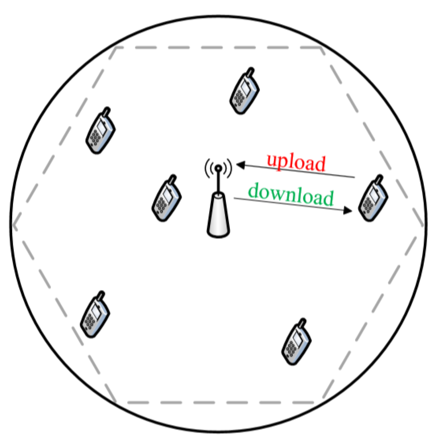
2.1. Overview and Assumptions

In this paper, we will consider a queuing system with elastic traffic and inpatient claims. To describe the flow of requests with a variable number of users, a Poisson flow of the first kind with the following parameters is suitable: the arrival intensity λ ( t ) , the minimum requirement for the resource b, and the length of the transmitted data block θ ( t ) . Table 1 reflects the main parameters that describe the system model and the corresponding terms of the mathematical model. In the system under consideration, there is a resource of volume C, a storage device with a finite capacity r. Requests also have the property of impatience—they leave the queue with intensity γ ( t ) . We will assume that the block length is equal to some value θ ( t ) . The entire volume C is divided equally between the orders, that is, if the number of customers is 1, then the entire resource is consumed by this customer, and the service rate is θ ( t ) / C ; if the number of customers is 2, then the service rate is 2 θ ( t ) / C —the resource volume is divided in half. In the case when C cannot be divided equally between the customers with the provision of the minimum guaranteed threshold b, a new customer enters the queue.
Let N ( t ) { 1 , , | C / b | } be the number of processed orders at the moment t 0 . Hence, the number | C / b | = N is the maximum number of requests that the device can process simultaneously. The state-space of the system looks like this:
X : = { n 0 , , N , , N + r : c ( n ) C } .

2.2. Continuous-Time Markov Chain

It is easy to see that the given model can be described by Markov process X ( t ) , t > 0 where X ( t ) denotes the number of customers in the system at time t (queue-length process). Denote by p n ( t ) = P ( X ( t ) = n ) , n = 0 , 1 , 2 , 3 , .
From the above assumptions, the resulting behavior of the state probabilities are described by a forward Kolmogorov system:
p 0 ( t ) = λ ( t ) p 0 ( t ) + C θ ( t ) p 1 ( t )
p n ( t ) = λ ( t ) p n 1 ( t ) C θ ( t ) + λ ( t ) p n ( t ) + C θ ( t ) p n + 1 ( t ) , 1 n < N
p N ( t ) = λ ( t ) p n 1 ( t ) C θ ( t ) + λ ( t ) p n ( t ) + C θ ( t ) + γ ( t ) p n + 1 ( t )
p n ( t ) = λ ( t ) p n 1 ( t ) C θ ( t ) + n N γ ( t ) + λ ( t ) p n ( t ) + C θ ( t ) + n + 1 N γ ( t ) p n + 1 ( t ) ,
N < n < N + r
p N + r ( t ) = λ ( t ) p N + r 1 ( t ) C θ ( t ) + r γ ( t ) + λ ( t ) p N + r ( t ) .
Now, we consider the corresponding nonstationary situation. Namely, we suppose that the queue-length process { X ( t ) , t 0 } is an inhomogeneous continuous-time Markov chain. All possible transition intensities say q i j ( t ) , are supposed to be non-random functions of time. We suppose that all intensity functions are nonnegative and locally integrable on [ 0 , ) .
Denote by p t = p 0 t , p 1 t , p 2 t , , p N + r ( t ) T the vector of state probabilities at the moment t. Put a i j t = q j i t for j i and a i i t = j i a j i t = j i q i j t .
We can consider the forward Kolmogorov system (2)–(6) as a differential equation
d p t d t = A t p t ,
in the space of sequences l 1 , where A t is a bounded for almost all t 0 linear operator from l 1 to itself and it is generated be the corresponding transposed intensity matrix:
λ ( t ) C θ ( t ) 0 · 0 0 0 · 0 0 λ ( t ) C θ ( t ) + λ ( t ) C θ ( t ) 0 0 0 0 0 0 λ ( t ) C θ ( t ) + λ ( t ) 0 0 0 0 0 0 0 0 C θ ( t ) + λ ( t ) C θ ( t ) 0 0 0 0 0 0 λ ( t ) C θ ( t ) + λ ( t ) C θ ( t ) + γ ( t ) 0 0 0 0 0 0 λ ( t ) C θ ( t ) + γ ( t ) + λ ( t ) 0 0 0 0 0 0 0 0 C θ ( t ) + ( r 1 ) γ ( t ) + λ ( t ) C θ ( t ) + λ ( t ) r 0 0 0 0 0 0 λ ( t ) C θ ( t ) + λ ( t ) r

2.3. Performance Measures

For analysis of the system let us consider some characteristics of the devoted model. First, the probability of blocking an incoming application:
P b l o c k ( t ) = p N + r ( t ) .
The average number of serviced applications:
C ¯ ( t ) = i = 1 N i p i ( t ) + N · i = 1 r p N + i ( t ) .
The average number of applications in the queue:
Q ( t ) = i = N + 1 N + r ( i N ) p i ( t ) .

3. Convergence Analysis

3.1. Definitions of Terms

We denote the mathematical expectation (the mean) of X ( t ) at the moment t if X ( 0 ) = k as E ( t , k ) = E X ( t ) X ( 0 ) = k .
The Markov chain X t is called weakly ergodic, if lim t p 1 t p 2 t = 0 for any initial conditions p 1 0 = p 1 Ω , p 2 0 = p 2 Ω . For our situation any p 1 t is considered as a quasi-stationary distribution of the chain X t .
The mentioned Markov chain X t also has the limiting mean ϕ ( t ) , if E ( t ; k ) ϕ ( t ) 0 as t for any k.
We recall the logarithmic norm of operator function from l 1 to itself is calculated as (12):
γ B t 1 = sup i b i i t + j i | b j i t | ,
and the bound
U t , s e s t γ B ( τ ) d τ ,
is valid for the Cauchy operator of the corresponding differential equation
d x d t = B ( t ) x .

3.2. Preliminary Considerations

Let us put that μ ( t ) = C θ ( t ) , and μ n ( t ) = μ ( t ) + max ( 0 , n N ) γ ( t ) for n 1 . Then
A ( t ) = λ ( t ) μ 1 ( t ) 0 0 0 λ ( t ) μ 1 ( t ) + λ ( t ) μ 2 ( t ) 0 0 0 λ ( t ) μ 2 ( t ) + λ ( t ) 0 0 0 0 0 μ N + r 1 ( t ) + λ ( t ) μ N + r ( t ) 0 0 0 λ ( t ) μ N + r ( t ) .
As indicated above, the considered method is based on the concept of the logarithmic norm and the corresponding estimates for the Cauchy operator.
Assuming that p 0 = 1 i = 1 N + r p i ( t ) , then from (7) we get the following equation:
d p d t = B t p + g t , t 0 ,
where g t = λ t , 0 , 0 , , 0 T and B t equals (17).
B t = μ 1 ( t ) + 2 λ ( t ) μ 2 ( t ) λ ( t ) λ ( t ) λ ( t ) λ ( t ) λ ( t ) λ ( t ) μ 2 ( t ) + λ ( t ) μ 3 ( t ) 0 0 0 0 λ ( t ) μ 3 ( t ) + λ ( t ) μ 4 ( t ) 0 0 0 0 0 0 μ N + r 1 ( t ) + λ ( t ) μ N + r ( t ) 0 0 0 0 λ ( t ) μ N + r ( t ) .
The solution to this equation can be represented in the following form:
p t = U t , 0 p 0 + 0 t U t , τ g τ d τ ,
where U t , s is the Cauchy operator of the corresponding homogeneous equation:
d x d t = B t x .
Next, we will consider estimates in "weighted" norms. Suppose d 1 , d 2 , , d N + r are positive numbers. Then let
D = d 1 d 1 d 1 0 d 2 d 2 0 0 d N + r .
We will denote by z 1 D = D z 1 . Note that B ( t ) is essentially non-negative, that is, all off-diagonal elements of B ( t ) are non-negative for any t 0 . Then we get:
B * * ( t ) = D B t D 1 = μ 1 ( t ) + λ ( t ) d 1 d 2 μ 1 ( t ) 0 0 0 d 2 d 1 λ ( t ) μ 2 ( t ) + λ ( t ) d 2 d 3 μ 2 ( t ) 0 0 0 d 3 d 2 λ ( t ) μ 3 ( t ) + λ ( t ) 0 0 0 0 d 4 d 3 λ ( t ) 0 0 0 0 0 μ N + r 1 ( t ) + λ ( t ) d N + r 1 d N + r μ N + r 1 ( t ) 0 0 0 d N + r d N + r 1 λ ( t ) μ N + ( t ) + λ ( t ) .
Let us put the following:
γ * * ( t ) = inf i | b i i ( t ) | j i d j d i b j i ( t ) .
Then we will get:
γ B ( t ) 1 D = γ D B ( t ) D 1 = sup i b i i ( t ) + j i d j d i b j i ( t ) = γ * * ( t ) .
For some positive δ we put d 1 = 1 , d k + 1 = δ d k , k 1 .

3.3. Bounds on the Rate of Convergence for Large Service Rates

First, we let δ > 1 . Then we will get the following:
α 1 ( t ) = μ 1 ( t ) + λ ( t ) δ λ ( t ) = μ ( t ) δ 1 λ ( t ) ,
α k ( t ) = μ k ( t ) + λ ( t ) 1 δ μ k 1 ( t ) δ λ ( t ) 1 1 δ μ k 1 ( t ) δ 1 λ ( t ) 1 1 δ μ ( t ) δ λ ( t ) , 2 k < N + r ,
α N + r ( t ) = μ N + r ( t ) 1 δ μ N + r 1 ( t ) + λ ( t ) 1 1 δ μ ( t ) δ λ ( t ) .
Therefore,
γ * * ( t ) = min α i ( t ) = 1 1 δ μ ( t ) δ λ ( t ) ) .
Theorem 1.
Let there be a positive number d e l t a > 1 such that,
0 ( μ ( t ) δ λ ( t ) ) d t = + .
Then the Markov chain X ( t ) is weakly ergodic and has the following convergence rate bounds:
p * ( t ) p * * ( t ) 1 D e 0 t 1 1 δ μ ( t ) δ λ ( t ) ) d τ p * ( 0 ) p * * ( 0 ) 1 D ,
p * ( t ) p * * ( t ) 4 δ N + r e 0 t 1 1 δ μ ( t ) δ λ ( t ) ) d τ p * ( 0 ) p * * ( 0 ) 8 δ N + r e 0 t 1 1 δ μ ( t ) δ λ ( t ) ) d τ ,
for any initial conditions p * ( 0 ) , p * * ( 0 ) and any t 0 .
We let that W = min k 1 d k k = min k 0 δ k k + 1 . Then we will get W p 1 E p 1 D .
Corollary 1.
From the conditions of Theorem 1, X ( t ) has a limit mean, then we say ϕ ( t ) = E ( t , 0 ) , and we obtain that the following estimate is true for any j and any t 0 :
| E ( t , j ) E ( t , 0 ) | 1 + δ j 1 W e 0 t 1 1 δ μ ( t ) δ λ ( t ) ) d τ .

3.4. Bounds on the Rate of Convergence for Large Arrival Rates

Now consider the case δ < 1 and assume that δ [ r 1 r , 1 ) . In this case, we have:
α 1 ( t ) μ ( t ) + ( 1 δ ) λ ( t ) ,
α k ( t ) 1 δ λ ( t ) + μ k ( t ) 1 δ μ k 1 ( t ) 1 δ λ ( t ) μ ( t ) 1 δ 1 , 2 k N + r 1
α N + r ( t ) λ ( t ) 1 δ 1 μ ( t ) .
Then it follows that we have the same:
γ * * ( t ) = min α i ( t ) = 1 δ 1 δ λ ( t ) μ ( t ) .
Theorem 2.
Let
0 δ λ ( t ) μ ( t ) d t = + ,
for some δ [ r 1 r , 1 ) . Then, the Markov chain X ( t ) is weakly ergodic and has the following convergence rate bounds:
p * ( t ) p * * ( t ) 1 D e 0 t 1 δ 1 ( δ λ ( t ) μ ( t ) ) d τ p * ( 0 ) p * * ( 0 ) 1 D ,
and
p * ( t ) p * * ( t ) 8 δ N + r e 0 t 1 δ 1 ( δ λ ( t ) μ ( t ) ) d τ ,
for any initial conditions p * ( 0 ) , p * * ( 0 ) and any t 0 . In addition, there is also a marginal mean and bound (29).
In addition, note the following: if the process is homogeneous (i.e., all intensities are constant), then the conditions of Theorems 1 and 2 are equivalent to the inequalities μ > λ and μ < λ , respectively.
And it is also worth noting that when all intensities of the process are 1-periodic, then there is a weak ergodicity X ( t ) and the estimates of Theorem 1 or Theorem 2 if:
0 1 λ ( t ) d t 0 1 μ ( t ) d t .

3.5. Perturbed CTMC and Bounds

In this subsection, we will consider the application of the general perturbation bounding in the same way as in the work [13]) for the models under study. We will consider a “perturbed” queue-length process X ¯ ( t ) , t 0 with the corresponding transposed intensity matrix A ¯ ( t ) , where the “perturbing” matrix A ^ ( t ) = A ( t ) A ¯ ( t ) is small. That is, we assume that the perturbed queue is of the same nature as the original one. Then the perturbed intensity matrix also has the same structure with the corresponding perturbed intensities θ ¯ ( t ) , γ ¯ ( t ) , λ ¯ ( t ) . We assume that μ ¯ n ( t ) = C θ ¯ ( t ) + max ( 0 , n N ) γ ¯ ( t ) for n 1 .
We suppose that:
1 θ ( t ) 1 θ ¯ ( t ) = 1 θ ^ ( t ) ϵ ^ , | γ ( t ) γ ¯ ( t ) | = | γ ^ ( t ) | ϵ ^ , | λ ( t ) λ ¯ ( t ) | = | λ ^ ( t ) | ϵ ^ .
Hence, we will get the following:
μ n ( t ) μ ¯ n ( t ) = | μ ^ n ( t ) | = | C θ ( t ) + max ( 0 , n N ) γ ( t ) C θ ¯ ( t ) max ( 0 , n N ) γ ¯ ( t ) | C θ ( t ) C θ ¯ ( t ) + max ( 0 , n N ) γ ( t ) γ ¯ ( t ) C ϵ ^ + r ϵ ^ = ( C + r ) ϵ ^ .
Then, from (8) we obtain the following bound:
A ^ ( t ) = 2 sup k a ^ k k t = 2 max | λ ^ ( t ) | , | λ ^ ( t ) | + | μ ^ n ( t ) | , | μ ^ N + r ( t ) | 2 C + r + 1 ϵ ^ .
Now from Theorem 1 and Corollary 1 in the paper [13] the following bounds of the perturbation follow.
Theorem 3.
Suppose that under the conditions of Theorem 1 or Theorem 2 the Markov chain X ( t ) is exponentially ergodic, that is,
e s t γ * * τ d τ K e γ 0 ( t s ) ,
for some positive K , γ 0 . Then the following bounds of the perturbation take place:
lim sup t p ( t ) p ¯ ( t ) 2 ϵ ^ C + r + 1 1 + log ( 4 K ) + ( N + r ) | log ( δ ) | γ 0 ,
and
lim sup t | E ( t , 0 ) E ¯ ( t , 0 ) | 2 ( N + r ) ϵ ^ C + r + 1 1 + log ( 4 K ) + ( N + r ) | log ( δ ) | γ 0 ,
for any perturbed queue with the respectively closed intensities satisfying to (36).

4. File Transfer in Wireless Network

4.1. Multi-Service Network

The system model of this work has the form of a cell, in the coverage area of which mobile devices are located (Figure 1). Each of them has its MSISDN (Mobile Subscriber Integrated Services Digital Number)—the mobile subscriber number of digital network with the integration of services. Each user behaves as follows: he sends a request to download a file, then downloads it, and also the user can disappear from the system. Disappearance can be associated with leaving the coverage area of the cell, or with a change in the type of service, or with the end of the service. The conclusion follows from the description of the system model: if we sum up the flow from all users, then the duration of the intervals between requests will not depend on the number of users, which is described by the Poisson flow of the first kind.
The users are provided with various services that belong to different categories of data transmission. A more detailed overview of the categories is illustrated in the Table 2. However, of these, we consider only those that can be described by elastic traffic, such as email, file transfer, and others.

4.2. Dataset Structure

The analysis of real traffic is of great importance, because the identification of the patterns of its arrival can make it possible to carry out studies of the system model described in the previous section in a non-stationary mode. Therefore, a task of this paper is formulated as follows: to analyze the traffic on one of the cell tower. There is a monitoring component to collect information about the system. Every hour, for each active device, the number of bits sent and received is added up. At the beginning of the next hour, the amount for the previous one hour is summed to the registration file. The principle of filling data during the monitoring is shown in Figure 2. There is a following designation S d , t u p —the sum of bits sent by the device per day d, at hour t. The part of the log file is shown in the Table 3. There are the column START_HOUR contains the full date and hour when the data was transferred; and the column MASKED_MSISDN—masked device identifier of the user; APP_CLASS—the class of the application that transfers data; UPLOAD—the number of bits, which were sent as we denoted S d , t u p ; and the last DOWNLOAD—the number of received bits as we denoted S d , t d o w n .

4.3. Daily Traffic Profile

We consider elastic traffic, which is characterized by such a parameter as the length of the elastic data block. For the considered traffic model, monitoring data were taken with a class “File Transfer”, which corresponds to the transfer of data using the FTP protocol.
To get the number of requests per second at a particular hour of the day for the selected application class, we perform aggregation of the form:
λ u p ( t ) = d S d , t u p 8 · 1024 · 1024 · l
λ d o w n ( t ) = d S d , t d o w n 8 · 1024 · 1024 · l ,
where the received sum is determined in bits, d—date and l—average packet size, equal to 2 MB. Then, we perform the calculation on Formulas (42) and (43) and the results are shown in Table 4.

4.4. Fourier Series Approximation

From the found values it is necessary to obtain some continuous function of the dependence of the fluctuation of the upward and downward traffic flows on the time of day. To do this, we perform approximation by the Fourier series. For clarity, we will gradually increase the number of conditions in a row, which is to choose the most optimal option.
Consider the dependence of the intensity of the upward data flow λ u p from time, and we will carry out the approximation by the Fourier series with one, two, and three conditions. As a result, we get a functions of the form (44)–(46) respectively and for our example the parameters will take values, which are shown in Table 5:
a ( t ) = a 0 + a 1 c o s ( w t ) + b 1 s i n ( w t )
a ( t ) = a 0 + a 1 c o s ( w t ) + b 1 s i n ( w t ) + a 2 c o s ( 2 w t ) + b 2 s i n ( 2 w t )
a ( t ) = a 0 + a 1 c o s ( w t ) + b 1 s i n ( w t ) + a 2 c o s ( 2 w t ) + b 2 s i n ( 2 w t ) + a 3 c o s ( 3 w t ) + b 3 s i n ( 3 w t ) .
Using Matlab, we have built the plots of the considered approximation. It is easy to see that the plot of the obtained approximation for the one condition (Figure 3a) differs significantly from the initial data, therefore, so that is why we increased the number of conditions to two and the graph of the resulting function for two conditions (Figure 3b) significantly reflects more faithfully the relationship between real data. Then, according to the plot of the approximation for the three conditions (Figure 3c), it could be seen that, now, in the intervals with the highest network load, the function has become closer to the real data points. However, in general, the graph did not receive significant changes, and the variant of the approximation with two conditions can be considered the most optimal.

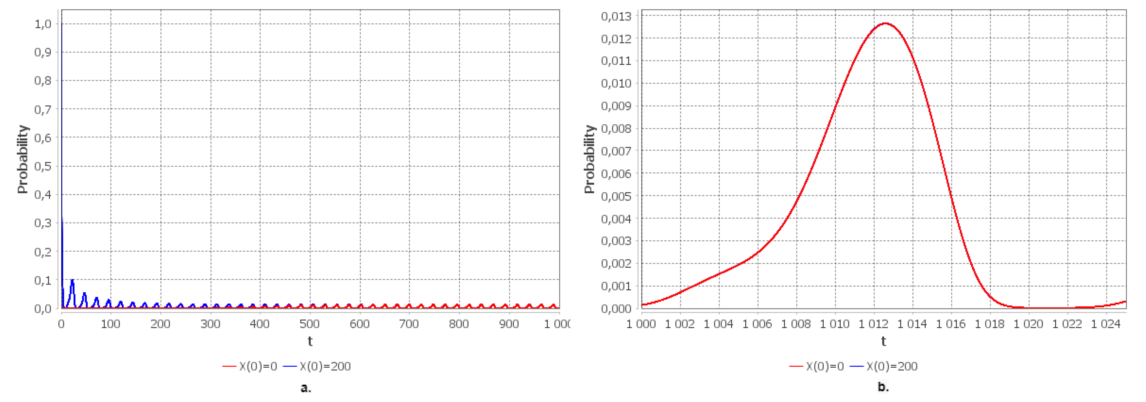
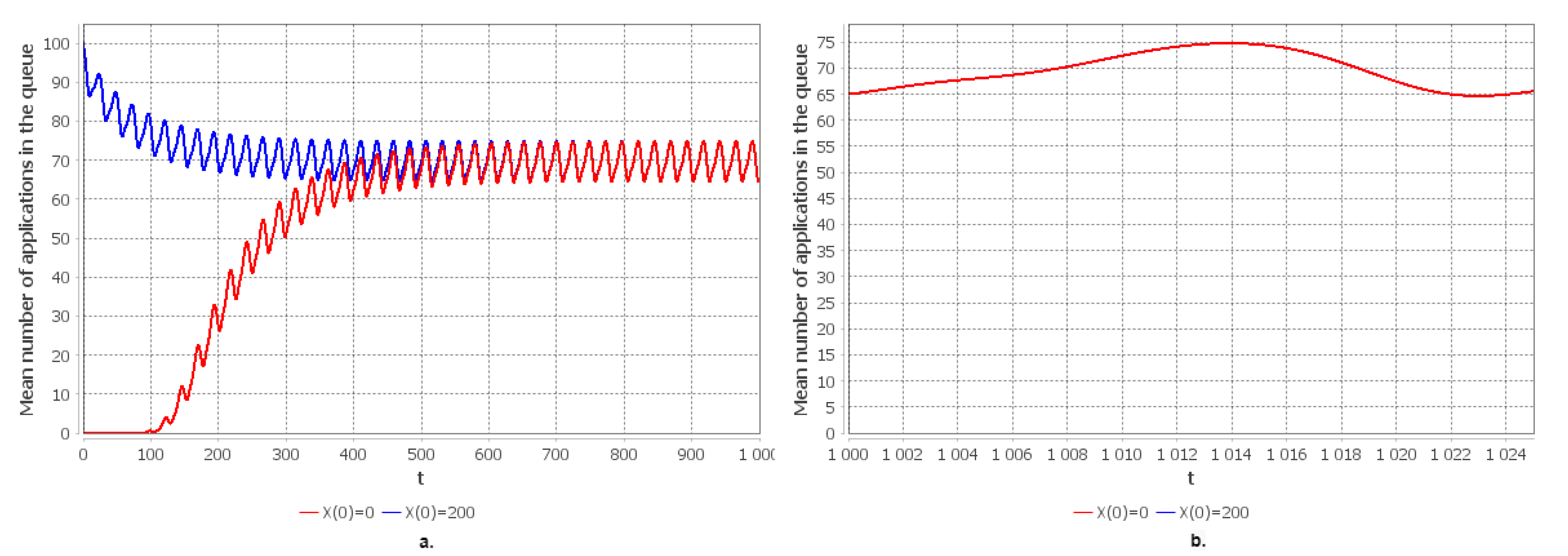
4.5. Numerical Analysis

For the numerical analysis, we will consider the following example: the volume of the resource block is C = 100 Mbps, and the finite capacity drive is r = 100 . The size of the transferred file equals to θ ( t ) = θ = 10 MB, that is 80 Mb, and the minimum transfer rate is b = 1 Mbps. The arriving intensity of device equals to λ ( t ) = λ · a ( t ) , where according to Section 4.4 a ( t ) equals to (46), where parameters are indicated in the Table 5 on the line for the third condition. The intensity of the flow of leaving requests for the transfer of a block of elastic data due to “impatience” is γ ( t ) = γ = 10 2 .
Apply all our bounds for this specific situation.
For applying of Theorems 2 and 3 we put δ = 0.99 , d 0 = 1 and d k + 1 = δ d k for k 0 . Then, we will get:
γ * * ( t ) = 1 99 2.97 ( a 0 + a 1 cos ( w t ) + b 1 sin ( w t ) + a 2 cos ( 2 w t ) + b 2 sin ( 2 w t ) + a 3 cos ( 3 w t ) + b 3 sin ( 3 w t ) ) 1.25 ,
e s t γ * * τ d τ e 0.016 ( t s ) ;
therefore, one can get K = 2 × 10 6 and γ 0 = 0.016 in (39).
Now we obtain the following bounds on the rate of convergence:
p * t p * * t 3 × 10 6 × e 0.016 t p * 0 p * * 0 ,
from Theorem 2;
p * ( t ) p * * ( t ) 1 D 2 × 10 6 × e 0.016 t p * ( 0 ) p * * ( 0 ) 1 D ,
| E ( t , j ) E ( t , 0 ) | 1 + 0.99 j 1 W e 0.016 t ,
from Theorem 2 and Corollary 1.
The corresponding perturbation bounds are:
lim sup t p ( t ) p ¯ ( t ) 5 × 10 5 ϵ ^ ,
and
lim sup t | E ( t , 0 ) E ¯ ( t , 0 ) | 10 8 ϵ ^ ,
from Theorem 3.
To solve the Cauchy problem, the 4th order Adams–Multon method was used with the use of IntelliJ IDEA software, JDK and the JFreeChart library, the functionality of which is used for plotting. The convergence plots were built for the characteristics specified in Section 2.3, shown in Figure 4, Figure 5 and Figure 6. To analyze the characteristics, two scenarios were chosen: 1. At the initial moment of time, our system is empty: X ( 0 ) = 0 ; 2. At the initial moment, the system is completely occupied, that is, all devices are occupied and there are no free places in the queue X ( 0 ) = 200 . Figure 4 shows graphs for the blocking probability. Note that, since we are considering two scenarios, then according to Figure 4a. for the first scenario, the starting value of the probability is 0, since the system is empty and it is logical that there will be no locks, and for the second scenario, the starting value is 1 since the system is completely busy. We can notice that the blocking probability for the two scenarios converges at time t = 500 and according to Figure 4b. We see that its values fluctuate within the range of 0.000 0.013 , and the period of fluctuation is 24. Further, in Figure 5, we see that the average number of service requests converges at 100; this may indicate a high load of devices in our system. However, the probability of blocking is small. Let us look at the average number of applications in the queue shown in Figure 6. As shown in Figure 6a. for the two scenarios, the graphs converge and the mean value is no less than 64 and no more than 75, as we can see in Figure 6b.

5. Conclusions

In this paper, we have investigated the process of downloading user files depending on the time in the form of a queuing system with elastic traffic and non-stationary intensities. We have developed a method for calculating the limits of convergence of such a model. Estimates of the rate of convergence are obtained based on the logarithmic norm of linear operators. As a result, it was found that the rate of convergence turned out to be low enough for an adequate representation of the situation in the limiting mode to begin at sufficiently long times. We evaluated the characteristics of such a model, namely, the probability of blocking new users, the average number of users downloading data, and the average number of users waiting for the download to start. We obtained the upper and lower bounds of their values.
We considered the model in the form of a single network slice and, in the framework of further tasks, we can consider the model in the form of several slices. If we want to scale our system, for example, to add another incoming stream, it will be necessary to solve the problem of redistribution; we will have to adapt our method for the new case. In addition, in our case, we have a one-dimensional random process, and for a new system where it will be multidimensional, we will first need to identify a function—a mapping, to go to the one-dimensional case to apply our method. This complexity can be viewed as a challenge for future research.

Author Contributions

Conceptualization, supervision, A.Z. and I.K. (Irina Kochetkova); methodology, Y.S. and I.K. (Irina Kochetkova); software, validation, visualization I.K. (Ivan Kovalev) and E.M.; investigation, writing, I.K. (Irina Kochetkova), Y.S., Ivan Kovalev, E.M., A.C., A.Z. All authors have read and agreed to the published version of the manuscript.

Funding

This research was funded by Russian Science Foundation, grant number 19-11-00020 (recipients I.K. (Irina Kochetkova), Y.S., I.K. (Ivan Kovalev), A.Z., Section 3, Section 4 and Section 5). This paper has been supported by the RUDN University Strategic Academic Leadership Program (recipients A.C., E.M., Section 1 and Section 2).

Institutional Review Board Statement

Not applicable.

Informed Consent Statement

Not applicable.

Data Availability Statement

Not applicable.

Acknowledgments

The authors are sincerely grateful to Luis M. Correia (IST/INESC-ID, University of Lisbon) for providing the dataset for Section 4.

Conflicts of Interest

The authors declare no conflict of interest.

References

  1. Kochetkov, D.; Almaganbetov, M. Using patent landscapes for technology benchmarking: A case of 5g networks. Adv. Syst. Sci. Appl. 2021, 21, 20–28. [Google Scholar] [CrossRef]
  2. Kochetkov, D.; Vuković, D.; Sadekov, N.; Levkiv, H. Smart cities and 5G networks: An emerging technological area? J. Geogr. Inst. Jovan Cvijic SASA 2019, 69, 289–295. [Google Scholar] [CrossRef] [Green Version]
  3. Barakabitze, A.A.; Ahmad, A.; Mijumbi, R.; Hines, A. 5G network slicing using SDN and NFV: A survey of taxonomy, architectures and future challenges. Comput. Netw. 2020, 167, 106984. [Google Scholar] [CrossRef]
  4. Khan, L.U.; Yaqoob, I.; Tran, N.H.; Han, Z.; Hong, C.S. Network Slicing: Recent Advances, Taxonomy, Requirements, and Open Research Challenges. IEEE Access 2020, 8, 36009–36028. [Google Scholar] [CrossRef]
  5. Muhizi, S.; Ateya, A.A.; Muthanna, A.; Kirichek, R.; Koucheryavy, A. A novel slice-oriented network model. Commun. Comput. Inf. Sci. 2018, 919, 421–431. [Google Scholar] [CrossRef]
  6. Ageev, K.A.; Sopin, E.S.; Yarkina, N.V.; Samouylov, K.E.; Shorgin, S.Y. Analysis of the network slicing mechanisms with guaranteed allocated resources for various traffic types. Inform. Primen. 2020, 14, 94–100. [Google Scholar] [CrossRef]
  7. Yarkina, N.; Gaidamaka, Y.; Correia, L.M.; Samouylov, K. An analytical model for 5G network resource sharing with flexible SLA-oriented slice isolation. Mathematics 2020, 8, 1177. [Google Scholar] [CrossRef]
  8. Kochetkova, I.; Vlaskina, A.; Burtseva, S.; Savich, V.; Hosek, J. Analyzing the effectiveness of dynamic network slicing procedure in 5g network by queuing and simulation models. Lect. Notes Comput. Sci. 2020, 12525, 71–85. [Google Scholar] [CrossRef]
  9. Vlaskina, A.; Polyakov, N.; Gudkova, I. Modeling and Performance Analysis of Elastic Traffic with Minimum Rate Guarantee Transmission under Network Slicing. Lect. Notes Comput. Sci. 2019, 11660, 621–634. [Google Scholar] [CrossRef]
  10. Vlaskina, A.S.; Polyakov, N.A.; Gudkova, I.A.; Gaidamaka, Y.V. Performance analysis of elastic traffic with minimum bit rate guarantee transmission in wireless network under network slicing, Izvestiya of Saratov University. Informatics 2020, 20, 378–387. [Google Scholar] [CrossRef]
  11. Gudkova, I.; Korotysheva, A.; Zeifman, A.; Shilova, G.; Korolev, V.; Shorgin, S.; Razumchik, R. Modeling and analyzing licensed shared access operation for 5G network as an inhomogeneous queue with catastrophes. In Proceedings of the International Congress on Ultra Modern Telecommunications and Control Systems and Workshops, Lisbon, Portugal, 18–20 October 2016; pp. 282–287. [Google Scholar] [CrossRef]
  12. Markova, E.; Satin, Y.; Kochetkova, I.; Zeifman, A.; Sinitcina, A. Queuing system with unreliable servers and inhomogeneous intensities for analyzing the impact of non-stationarity toperformance measures of wireless network under licensed shared access. Mathematics 2020, 8, 800. [Google Scholar] [CrossRef]
  13. Zeifman, A.; Korolev, V.; Satin, Y. Two approaches to the construction of perturbation bounds for continuous-time Markov chains. Mathematics 2020, 8, 253. [Google Scholar] [CrossRef] [Green Version]
  14. Zeifman, A.; Satin, Y.; Kryukova, A.; Razumchik, R.; Kiseleva, K.; Shilova, G. On the Three Methods for Bounding the Rate of Convergence for some Continuous-time Markov Chains. arXiv 2020, arXiv:1911.04086. [Google Scholar]
  15. Arns, M.; Buchholz, P.; Panchenko, A. On the numerical analysis of inhomogeneous continuous-time Markov chains. Informs J. Comput. 2010, 22, 416–432. [Google Scholar] [CrossRef]
  16. Andreychenko, A.; Sandmann, W.; Wolf, V. Approximate adaptive uniformization of continuous-time Markov chains. Appl. Math. Model. 2018, 61, 561–576. [Google Scholar] [CrossRef]
  17. Katoen, J.-P.; Zapreev, I.S. Safe on-the-fly steady-state detection for time-bounded reachability. In Proceedings of the 3rd International Conference on the Quantitative Evaluation of Systems, California, CA, USA, 11–14 September 2016. [Google Scholar]
Figure 1. Scheme of System Model.
Mathematics 10 00030 g001
Figure 2. The principle of data accumulation during monitoring.
Mathematics 10 00030 g002
Figure 3. (a) Graph of the approximation function a ( t ) for upward flow with one condition; (b) Graph of the approximation function a ( t ) for upward flow with two conditions; (c) Graph of the approximation function a ( t ) for upward flow with three conditions.
Mathematics 10 00030 g003
Figure 4. (a) Probability of blocking for t [ 0 , 1304 ] . (b) Approximation of the limiting probability of blocking for t [ 1304 , 1329 ] .
Mathematics 10 00030 g004
Figure 5. (a) The mean of applications served E ( t , k ) for t [ 0 , 1304 ] . (b) Approximation of the limiting mean of applications served E ( t , k ) for t [ 1304 , 1329 ] .
Mathematics 10 00030 g005
Figure 6. (a) The mean of applications in the queue Q ( t ) for t [ 0 , 1304 ] . (b) Approximation of the limiting mean of applications in the queue Q ( t ) for t [ 1304 , 1329 ] .
Mathematics 10 00030 g006
Table 1. System model parameters.
ParameterDescription
λ ( t ) Intensity of the flow of requests for the transfer of elastic data
bMinimum guaranteed elastic data block transfer rate
θ ( t ) Average value of data block length
rThe queue of applications for the transfer of a block of elastic data
γ ( t ) The rate of loss of impatient claims
CNetwork bandwidth (service speed)
Table 2. Description of service types.
N.Service NameDescription
1DB TransactionsTransaction in a database—for example, transfer of funds from a credit card through a mobile application.
2File SystemsWork with remote file systems. This is how ATMs are arranged, for example. There is a machine with an operating system, and ATMs are connected to it and all information is stored there.
3File TransferFile transfer via FTP.
4GamesOnline game traffic.
5Instant Messaging ApplicationsInstant messaging systems - messengers WhatsApp, Viber, Telegram, etc.
6Legacy ProtocolsDeprecated protocols.
7MailEmail.
8Music StreamingStreaming services for listening to music.
9Network OperationNetwork services.
10OthersOthers
11P2P ApplicationsApplications where data transmission is based on the principles of peer-to-peer networks. The simplest example is Bittorrent applications.
12SecurityOnline video cameras, data from alarm sensors, etc.
13Streaming ApplicationsStreaming services for watching movies and video-chats.
14TerminalsMobile terminals for credit card payments.
15VoIPIP-telephony. For example, calls via WhatsApp or Skype.
16Web ApplicationsWeb applications—client-server applications in which the client interacts with the server using a browser (Microsoft Office Online, Google Documents).
Table 3. Part of the log file.
START_HOURMASKED_MSISDNAPP_CLASSUPLOADDOWNLOAD
12.02.2018 10:009BFA3001DE8C58C2453B6
9CE2E4A3704
Web Applications111,33978,208
12.02.2018 8:000C2C88351A593CD02727A
6207EB85E9E
Instant Messaging Applications11,9466741
12.02.2018 10:00B9F45E1542162096408D9
4DD94499B89
Web Applications67,143,8324,230,675
12.02.2018 10:003CF6B81BC186E4C188D69
E1FE8919BB6
Web Applications18,8449769
11.02.2018 18:007EE1FCE60945D869A14EF
30E896E9131
Streaming Applications17,219,335403,361
11.02.2018 17:00A746CCDCAC507B95C83
A3475C63C6BFD
Web Applications235,455131,712
11.02.2018 16:00EA9D75DEB103F439A8C2
8300C2CC1757
Streaming Applications136,767,0004,078,817
12.02.2018 9:00610FF30F1C9EC8939B4F
BD259255BD63
Streaming Applications3,330,234112,395
12.02.2018 10:006DFD256C104B394A884E0
6A6EF7BE156
File Transfer26,804,5782,111,659
11.02.2018 17:006C9A6A5D444E7416C0C43
10E617EB611
Web Applications587,78687,897
Table 4. Dependence of the number of requests on the time of day.
Times of Day, t λ up ( t ) λ down ( t )
00.4848474940.040711044
10.3418659430.031079608
20.1908232620.018468431
30.1321430120.013982313
40.1186978440.011683847
50.1058035650.009923712
60.1164745260.012585431
70.2429420930.019329354
80.5486778370.045828017
90.8824842750.062668489
100.9163285380.091028611
110.9202438220.087240118
120.8148160020.08172834
130.7100776120.0853086
140.8201035860.095698016
150.8793270480.090266848
160.9512043910.098226292
170.9459084330.09180442
180.9900045160.082148071
190.9918903880.074312104
200.9076433250.067218977
210.9575844880.066221158
220.9266372060.112652817
230.7551756350.067874847
Table 5. Parameters of Fourier Series Approximation for the upward data flow.
Conditionw a 0 a 1 b 1 a 2 b 2 a 3 b 3
one0.25190.6472−0.168−0.3675
two0.26170.6521−0.07656−0.39920.1479−0.1348
three0.26030.6521−0.08888−0.39630.1384−0.1411−0.014460.05875
Publisher’s Note: MDPI stays neutral with regard to jurisdictional claims in published maps and institutional affiliations.

