
School Timetabling Optimisation Using Artificial Bee Colony Algorithm Based on a Virtual Searching Space Method


1
School of Engineering & Technology, CQ University, Rockhampton 4701, Australia
2
Tertiary Education Division, School of Engineering & Technology, CQ University, Rockhampton 4701, Australia
*
Authors to whom correspondence should be addressed.
Mathematics 2022, 10(1), 73; https://0-doi-org.brum.beds.ac.uk/10.3390/math10010073
Submission received: 6 November 2021
/
Revised: 17 December 2021
/
Accepted: 21 December 2021
/
Published: 26 December 2021
(This article belongs to the Special Issue Recent Advances in Multiple Criteria Decision Making Approaches)
Abstract
:Although educational timetabling problems have been studied for decades, one instance of this, the school timetabling problem (STP), has not developed as quickly as examination timetabling and course timetabling problems due to its diversity and complexity. In addition, most STP research has only focused on the educators’ availabilities when studying the educator aspect, and the educators’ preferences and expertise have not been taken into consideration. To fill in this gap, this paper proposes a conceptual model for the school timetabling problem considering educators’ availabilities, preferences and expertise as a whole. Based on a common real-world school timetabling scenario, the artificial bee colony (ABC) algorithm is adapted to this study, as research shows its applicability in solving examination and course timetabling problems. A virtual search space for dealing with the large search space is introduced to the proposed model. The proposed approach is simulated with a large, randomly generated dataset. The experimental results demonstrate that the proposed approach is able to solve the STP and handle a large dataset in an ordinary computing hardware environment, which significantly reduces computational costs. Compared to the traditional constraint programming method, the proposed approach is more effective and can provide more satisfactory solutions by considering educators’ availabilities, preferences, and expertise levels.
1. Introduction
The problem of timetabling can be defined as a computational problem that allocates resources in given periods under particular constraints to achieve desirable goals [1]. Educational timetabling is one of the fundamental tasks affecting educational institutes’ operations and productions. Educational timetabling problems (ETPs) are constraint satisfaction problems involving multiple aspects, such as educators, students and educational resources. Based on the types of educational activities, ETPs can be roughly categorised as course timetabling, examination timetabling and school timetabling problems [2]. Course timetabling arranges educational facilities, such as classrooms and laboratories, ensuring no single student takes more than one course at the same time and no classroom hosts more than one class at a time. Examination timetabling prevents an individual student from taking more than one exam simultaneously but allows exams to share rooms and/or invigilators. Generally, the problem of the school timetabling is to allocate educators to classes with the considerations of their availability and expertise [3], which is the focus of this study.
School timetabling problems (STPs) have been recognised as a non-polynomial (NP) complete problem, as its variables vary from one educational institute to another [4], and therefore, the efficient solution algorithms for this problem have not been found [5]. Although STPs have been studied since the 1960s [6], this area has not been developed as quickly as course timetabling and examination timetabling problems, likely because of the isolation of studies in particular schools [7]. In addition, the wide variety of school timetables complexifies the problems. For example, some schools [8,9] treat courses, educators and rooms as resources to be allocated, whereas some schools bind courses and educators as a pair to be assigned [9,10].
To solve STPs, many computational intelligent methods and approaches have been applied, which are mainly categorised as heuristic approaches and novel approaches [11,12]. Heuristic approaches consist of metaheuristics and hyper-heuristics. Metaheuristics approaches are inspired by natural phenomena, aiming at seeking better solutions rather than the best solution [13,14]. Hyper-heuristics uses metaheuristics methods to select a metaheuristic to solve generalised solutions [15]. Novel approaches include hybrid approaches, fuzzy logic approaches and MAS. Hybrid approaches employ different methods to solve a problem in order to alleviate the weakness of a single method [16,17]. Fuzzy logic approaches aim to solve those problems which are hard to be quantitated and modelled as they do not have a precisive classification [18,19]. MAS deploys serval computational intelligent methods as an agent to play different roles to collaboratively fulfil a common goal [20].
Based on the abovementioned approaches, many applications are developed to solve STPs. In the metaheuristics field, Odeniyi, Omidiora, Olabiyisi and Aluko proposed a modified simulated annealing approach for Fakunle Comprehensive High School in Nigeria [21]. With the aid of the annealing scheme through the temperature parameter introduction, the approach successfully reduced the convergence time and computational cost brought by the annealing algorithm in dealing with large search spaces. A simple genetic algorithm (SGA) was adopted by Sutar and Bichkar [22] to solve an STP with knowledge-augmented operators and probabilistic repair in the crossover step. The result of the modified approach against the OR-Library dataset [22] suggested that SGA could produce faster solutions for GA-based optimisation problems than the conventional GA method. In the hyper-heuristics area, Ahmed, Ozcan and Kheiri [23] combined five different selection hyper-heuristics with three-move acceptance methods to challenge the ITC2011 instances. The outcome indicated that the approach was better than evolutionary algorithms [24] and an adaptive large neighbourhood search algorithm [25] but not when compared to hybridised simulated annealing (SA) and stagnation-free late acceptance hill climbing [26]. Hybrid approaches are combinations of various approaches. Those combined approaches for solving STPs include, but are not limited to, cat swarm optimisation (CSO) with a local search algorithm [27] and particle swarm optimisation (PSO) with hybrid artificial fish swarm (AFS) [28]. Babaei, Karimpour and Oroji employed a fuzzy c-means clustering algorithm to solve STPs for Islamic Azad University [29] to reduce redundancy and consider lecturers’ preferences. When school timetabling is being planned, it will get multiple stakeholders involved, such as educators, heads of school and administrators, to negotiate. Therefore, MAS is often applied to simulate the process and the parties of the negotiations. Oprea [30] demonstrated that MAS could handle the negotiations between faculties and minimise resource conflicts, while Tkaczyk, Ganzha and Paprzycki [31] emulated the school timetabling workflow of the University of Gdansk with MAS.
Although many efforts have been made in the educational timetabling research field for decades, there has still been no consensus about the standard formulation and data format [9]. In addition, most STP research has only focused on educators’ availabilities when they studied the educator aspect [7,32], and the attributes of educators’ preferences and expertise were not taken into consideration. To address this issue, this paper chooses a common real-world school timetabling scenario to study and takes educators’ preferences towards units (also known as “courses” in some literature) and the corresponding expertise level into account. Based on the chosen scenario, this paper presents a model of the STP and proposes a modified ABC algorithm to solve the problem. Although, to the authors’ best knowledge, ABC has not been applied to STPs, it has potential in tackling STPs, as it has successfully solved ETPs in the course [33,34] and examination [16,35,36] timetabling fields. In addition, this paper introduces a novel VSS method to reduce search space. The proposed approach is simulated with a randomly generated large dataset. The experiment results demonstrate that the proposed approach is able to solve the STP and handle a large dataset in an ordinary computer hardware environment.
The contributions of this research include a conceptual model and its mathematical formulation for the STP, considering educators’ availabilities, preferences and expertise as a whole; a novel VSS method for reducing the computational cost of handling a large searching space; and a modified ABC algorithm to solve the proposed STP model.
The organisation of this article is as follows. Section 2 presents the problem formulation, including a conceptual model of the STP, identification of hard and soft constraints and formulation of the objective function. Section 3 presents a review of the related bio-inspired optimisation methods. Section 4 describes the proposed approach, consisting of a concept of educator allocation, a modified ABC algorithm and a VSS construction method. Section 5 simulates the proposed approach with a case based on a local university’s business scenario. A comparison study between the proposed approach and the Constraint Programming (CP) is presented in Section 6. Section 7 concludes the article and indicates future works.
2. Problem Formulation
As the descriptions and terminology of STP are dramatically different from study to study [7], this section firstly defines the STP studied and the terms used in this paper. After that, hard constraints and soft constraints of the STP will be identified, followed by the objective function formulation.
2.1. Terminology
A course refers to an academic program that students need to learn to gain university degrees; for example, in a Bachelor of Mobile Application degree, Mobile Application is the course name.
A unit refers to the academic subject within a course, e.g., Java programming is a unit of the course Mobile Application.
A class refers to the particular teaching activity being scheduled in a timeslot in a day, which could be a lecture, a tutorial, a workshop and/or other educational activities.
An educator refers to the educational staff who delivers lectures, tutorials, workshops, etc.
A school week is from Monday to Friday.
A school day is a day of a school week.
2.2. School Timetabling Concept Model
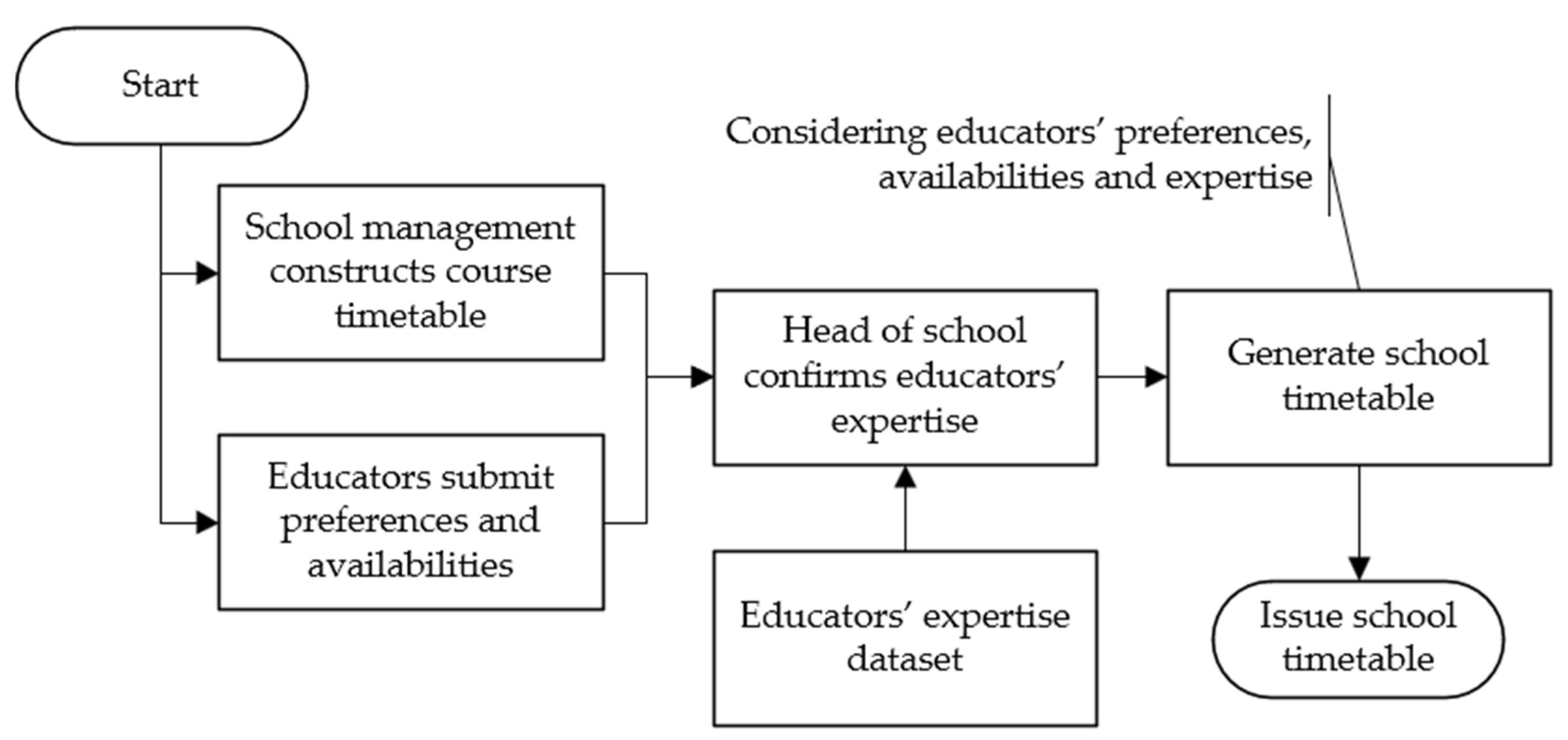
In this study, three parameters of educators have been taken into consideration: preferences, availabilities and expertise. The objective of the school timetabling is to allocate all the school educators to a scheduled course timetable that satisfies all the preferences, availabilities and expertise as much as possible. The conceptual model of the school timetabling is presented in Figure 1. In the beginning, a course timetable is preconstructed according to all university course information. That is, all the class activities have been scheduled with their timeslots in a school week. The course timetable has ensured that every single student will not take more than one unit at the same time. Educators provide their availabilities in a school week and their preferences, along with preference levels, against each unit. After that, the head of school will generate a school timetable by allocating educators to the scheduled course timetable according to educators’ availabilities, preferences and expertise. The level of expertise against units is predefined by the head of school.
2.3. Symbols and Notations
Parameters
| L | Total number of educators |
| O | Total number of units |
| K | Total number of classes in a school week |
| P | Maximum preference value |
| E | Maximum expertise value |
| V | Number of classes that an educator is allowed to deliver in a school week |
| H | Number of hours in a school day (e.g., from 8:00 a.m. to 6:00 p.m., there are 10 h) |
| D | Number of days in a school week |
| M | Maximum number of hours a class lasts |
Variables
| d | |
| t | |
| r | |
| c | |
| p | * |
| e | * |
| A | |
| u | Number of units that cannot be allocated with educators |
| * When p = 0, it indicates that an educator does not prefer a unit. When e = 0, it means that the educator is not capable to deliver the unit. By default, all the p and e are 0. They need to be set by educators and the head of school. | |
Notation
| Set of timeslots that educator is available in the school week. If educator is available during a whole school week, then . | |
| Set of timeslots that class is scheduled to in the school week. If class is scheduled in the first three hours of the school week, then . |
2.4. Hard Constraints
Hard constraints are those conditions that the solutions have to satisfy. In this study, the hard constraints listed below are binary values. If a hard constraint is violated, it will be given value zero; otherwise, value 1 will be assigned. The hard constraints are notated as and mathematically modelled as below:
No educator can deliver more than one class simultaneously.
where
: An educator will only be assigned to the timeslots of a class when s/he is available. Meanwhile, the class must be fully allocated to an educator, meaning that the allocated educator must be available during the whole period of the class.
: One class only can be allocated with one educator.
where is the index of classes and j is the index of the educators; are decision variables, which is explained in Equation (6).
: No educator is allowed to teach more than V classes in a school week.
where i is the index of classes and j is the index of the educators; are decision variables, which is explained in Equation (6).
2.5. Soft Constraints
Soft constraints are those conditions that the solutions do not have to satisfy but are preferably satisfied. The following soft constraints have been identified:
- Educators will be assigned to the most preferred units.
- Units will be allocated to the educators who are more capable to teach.
- All units must be allocated to educators.
In practice, some units cannot be allocated with educators—for example, when a unit has not been favoured by any educator, or when two units are only favoured by one educator, but these two units are time-conflicted.
2.6. Objective Function
The objective of this study is to maximise both all educators’ satisfaction and all units’ quality of teaching, or in other words, to let the units be taught by the most qualified educators and to let the educators teach their most preferred units. When a unit is allocated to an educator, its allocation quality will be decided by the educator’s expertise level and associated preference level, subject to the hard constraints being satisfied. This study defines the objective value of a class allocation as shown in Equation (5), which is the multiplication of preferences () and expertise () values given to class .
where refers to the preference of educator toward class ; represents the expertise of educator to class .
According to the concept model, the course timetable is preconstructed. The STP can be transferred to an allocation problem. Figure 2 is the bipartite graph for the STP.
The objective function for school timetabling is to maximise the sum of every class’s objective value ().
Therefore, the STP optimisation model can be presented as follows.
Maximise:
subject to:
where:
u is the number of unallocated units (if all the units are allocated, then u will be set to be 1).
3. Related Bio-Inspired Optimisation Methods
The ABC algorithm belongs to bio-inspired optimisation methods. This section presents a review of related bio-inspired optimisation methods, aiming for providing a reference for future research.
ETPs have been studied over five decades in computational intelligence areas [37]. Most of the approaches and methodologies introduced and developed in the studies fall into heuristics algorithms [38]. In a heuristic algorithm catalogue, population-based approaches were experimentally proven to be suitable for solution search space exploration [39], which aligns with the objective of this research to seek an optimal solution. Population-based algorithms can be categorised into evolution-inspired, physical-phenomenon-inspired and bio-inspired approaches. To some extent, bio-inspired approaches have better performance over the other two groups [40,41]. Consequently, this research chose a bio-inspired approach in applying to the proposed model.
Under the umbrella of bio-inspired algorithms, the popular ones are the particle swarm optimisation [42] (PSO) algorithm, the ant colony optimisation (ACO) [43], the artificial fish swarm algorithm [44] (AFS), the whale optimisation algorithm [40] (WOA), the firefly algorithm [45], the shuffled frog leaping (SFL) [46] algorithm and the artificial bee colony (ABC) [33] algorithm. The PSO algorithm was introduced in 1995 by Kennedy and Eberhart [42], inspired by the food-searching behaviour of bird flocks. It is easier to implement, with fewer parameters to control, and is good at dealing with multidimensional complex space [47]. The ACO algorithm simulates the foraging behaviours of ants with the feature of the indirect communication of ant groups [48]. It is suitable for complex combinational optimisation. AFS gets inspiration from the collective movement and the schooling behaviours of fish. It possesses advantages including high convergence speed, flexibility, error tolerance and high accuracy. However, its disadvantages, such as high time complexity and imbalance between global and local search, have to be mitigated by using AFS in combination with other algorithms [44]. Inspired by the hunting behaviour of humpback whales, WOA uses encircling prey, bubble-net attacking and searching for prey to populate, exploit and explore optimal solutions, respectively. WOA is able to seek solutions in unknown searching spaces [40]. The firefly algorithm unconventionally populates numerous agents instead of searching randomly, which helps agents effectively explore search spaces. As a result, the firefly algorithm can effectively solve multi-objective optimisation [45]. Though the ABC algorithm [33] has been widely studied for solving educational timetabling problems, especially solving course timetabling problems [34,49,50] and examination timetabling problems [35,36,51], it has not been applied to STPs. Therefore, this research adapts the ABC algorithm to the proposed problem, which will be introduced in detail in Section 4.2 and Section 4.3.
4. The Proposed Approach
This section firstly presents a basic concept of allocating educators to the scheduled course timetable. Based on the concept, a modified ABC algorithm is introduced. After that, a novel method named VSS is proposed to solve the gigantic searching space issue.
4.1. The Basic Concept of Educator Allocation
The research aims to allocate educators to a scheduled course timetable and attempts to satisfy their availabilities, preferences and expertise as much as possible. The allocation concept can be illustrated in Figure 3.
In Figure 3, the left side is an example of a scheduled course timetable, listing the classes along with their weekdays, start times and durations. The educator ID column is to be filled with the IDs of the educators who are allocated to the classes. Weekdays and start times indicate which weekday the class is allocated to and at what time the class will start. Duration shows how long the class will last. On the right side of Figure 3, the educator list is presented, including educator ID, preference and expertise and availability columns. The educator ID column lists educators’ IDs ; the preference and expertise column stores a two-dimensional table, exampled in Table 1, which has K rows and three fields storing all the unit IDs, as well as the preferences and the expertise levels of an educator against those units. If an educator has no interest in teaching a class, for example, in Table 1, then the preference and expertise will be filled with 0; otherwise, the corresponding level number will be input. The availability column contains a one-dimensional array converted from the two-dimensional school week timetable exampled in Table 2. The number of elements in the availability array is . The availability column indicates the availabilities of each educator in a school week. If an educator is available at, for example, 8:00 a.m. on Monday in Table 2, then the first cell of the array will be marked with a Y; otherwise, an N will be stored.
The basic process of allocating educators is to match each educator against a unit. Figure 3 can be used as an example to explain the process. Assume that is capable (“capable” means the expertise value is not equal to zero) and available to teach , and are capable to teach and , but only is available to teach . Firstly, the program will consult the first unallocated educator from the educator list, which is , and allocate it to the first unallocated class, which is , as is capable and available. Then, the corresponding cell on ’s availability table will be marked with “N”. After that, becomes the first unallocated educator. However, is not available to teach , and therefore the consecutive unallocated educator, that is, , will be consulted. As is capable and available, will be assigned to . When ’s allocation is finished, becomes the first unallocated educator and will be consulted for the . As is capable and available to teach , thus takes . When all the educators and their profiles have been consulted, a timetable solution would be outputted.
With the concept of educator allocation, it is known that a specific educator list sequence subjected to the course timetable will always output the same school timetable. For instance, in Figure 3, educator will always be assigned to the class , even if educator might be more suitable (e.g., has a higher value than ), as will be consulted before . Therefore, an educator list can be considered as a solution, and therein changing the educator list sequence can obtain different solutions, from which it can be reasoned that the number of possible solutions is the number of permutations of the educator list or, in other words, is the factorial of the number of educators. All of the possible solutions form the entire solution searching space. However, the number of educators in a university could be over 100, meaning that the number of solutions would be gigantic and lead to the impossibility of seeking the best solution by traversing the whole searching space. Therefore, an artificial intelligence algorithm is needed.
4.2. ABC Algorithm
The ABC algorithm was chosen for the proposed STP for its ability to solve multivariable, multimodal optimisation problems efficiently. Additionally, the ABC algorithm can be easily implemented without requiring many parameters. The ABC algorithm is inspired by the behaviours of honeybees and was introduced by Karaboga [52]. It simulates the ways that honeybees forage for food sources, which helps bees efficiently and effectively seek better food sources in a vast area. The mechanisms the ABC algorithm uses include positive feedback, negative feedback, fluctuations and multiple interactions. These four mechanisms help the bees to explore new food sources and to avoid over-populating a source, as well as to ensure information can be shared with each bee. Labour division is another feature of the ABC algorithm. Bees are categorised to be employee bees, onlooker bees and scout bees. Employee bees are responsible for new food source exploration; onlooker bees are in charge of food source analysis and exploitation; scout bees avoid food source exhaustion.
The ABC algorithm consists of four stages: population, employee bee, onlooker bee and scout bee stages.
In the solution population stage, the ABC algorithm randomly populates several solutions (bees) in a searching space with Equation (7).
where i is one of the nodes in the searching space and d is dimension. and are the upper bound and lower bound, respectively, for the dimension d.
In the employee bee stage, neighbours of the populated solutions will be looked for with Equation (8).
where k is randomly chosen from the searching space and k ≠ 1. is randomly generated in the range of [–1, 1]; is a neighbour of . The probability of each employee bee will be calculated with Equation (9).
In the onlooker bee stage, a random number [0, 1] will compare to for each employee bee, and if the random number is better than a , an onlooker bee will be sent to look for a neighbour of the employee. A parameter called trail will be used in this stage. Trail limits the times that a food source has been explored. If the exploration time reaches the trail and the better neighbour has not been found, the food source will be abandoned.
In the scout bee stage, the onlooker bee(s), whose food source(s) is/are abandoned, will become scout bee(s) and randomly populate a new solution. The equation scout bees use is similar to Equation (7).
4.3. A Modified ABC Algorithm for Proposed STP
The modified ABC algorithm is presented in Algorithm 1. To adapt the ABC algorithm, some modifications have been made to suit the investigated problem. The modifications are described as follows.
| Algorithm 1. Pseudocode of the modified ABC algorithm. |
| /*Initialisation stage*/ 01: Retrieve the scheduled course timetable and educators’ profiles 02: Define the neighbour search range, number of Traits and read parameters 03: Initialise the food source and construct school timetable, satisfying all hard constraints as in Equations (1)–(4) 04: Evaluate school timetable’s objective values with Equation (6) 05: Send the employed bees to the current food sources 06: Iteration = N 07: FOR (each iteration) /∗Employed Bee Phase∗/ 08: FOR (each employed bee) 09: Seek new food source from neighbourhood in VSS, satisfying Equations (1)–(4) 10: Construct school timetables and evaluate their objective value with Equation (6); apply greedy selection 11: END FOR 12: Calculate the probability p for each food source with Equation (9) /∗Onlooker Bee Phase∗/ 13: FOR (each onlooker bee) 14: Send onlooker bees to food sources based on p 15: Find a new food source in its neighbourhood in VSS, satisfying Equations (1)–(4) 16: Construct school timetables and evaluate their objective value with Equation (6); apply greedy selection and set Trait + 1 if applicable 17: END FOR /∗Scout Bee Phase∗/ 18: IF (any onlooker bee becomes scout bee) 19: Send scout bee to a randomly produced food source, satisfying Equations (1)–(4) 20: END IF 21: Memorise the best solution achieved so far 22: END FOR 23: Output the best solution achieved |
Before food source initialisation, a scheduled course timetable will be retrieved from the course database, followed by the educator profiles data retrieval (Step 1 in Algorithm 1). The examples of a course timetable and an educator profile are illustrated in Figure 3. Since the boundary (Equations (7) and (8)) of the searching space and the current neighbourhoods need to be known when bees are foraging for food sources, the searching space will be formed beforehand. However, as mentioned before, the number of solutions is gigantic, so this research proposes a VSS to tackle this dilemma. The VSS is detailed in Section 4.4. To construct the final solutions from the food sources that bees forage from the VSS (Step 03, 09, 15 and 19 in Algorithm 1), the school timetable construction will be applied and detailed in Section 4.5. The objective values of constructed final solutions will be evaluated with Equation (6) (Steps 04, 10 and 16 in Algorithm 1).
The major modifications are summarised as below:
- Integrate VSS construction approach in neighbour population process (Steps 9 and 15 in Algorithm 1) instead of forming a whole searching space beforehand.
- Integrate school timetable constructor approach to generate solutions in every objective value evaluation process (Steps 3, 10 and 16 in Algorithm 1) instead of picking up solutions directly when populate.
4.4. Virtual Searching Space Construction
VSS aims to provide an entire solution pool for the proposed algorithm rather than constructing a gigantic searching space. As discussed above, the searching space is formed through permutation manipulation with the magnitude of the factorial number of educators. Thus, it would be impractical to physically construct the whole searching space, as it would exceed the memory capacity of ordinary computers, not to mention the computational time for generating all the solutions for each educator list. To tackle this dilemma, we propose a novel VSS approach. VSS does not construct a searching space by the direct permutations. Instead, it “imagines” the solutions to be allocated in the searching space in the way exampled in Table 3.
4.4.1. How VSS Works
Assume one bee is employed and four educators are to be allocated, in which case the searching space will be similar to Table 3 with four regions (A, B, C and D) and twenty-four possible solutions (hereafter referred to as columns) numbered.
In the food source initialisation phase (Step 03 in Algorithm 1), VSS does not need to know the solutions’ coordinators in the searching space, as any educator list combination will be in the solution pool. VSS randomly generates an educator sequence B-A-D-C (Column 8).
In the neighbour-seeking phase, VSS swaps the positions of A and C in Column 8 to obtain Column 10. The swap method can decide the distance, vector and boundary of neighbour solutions with the following rules:
Rule 1: Fixing top element(s) can confine the boundary of the neighbourhood. For example, when the first element “B” is fixed, the neighbourhood will be in B region. When “B-A” is fixed, there are only two neighbours, B-A-C-D (Column 7) and B-A-D-C (Column 8). This rule confines the upper bound and lower bound for a dimension as and in Equation (7).
Rule 2: The relationship of swapping elements determines the orientation. For example, if the higher element (A) switches with the lower one (C) (in practice, higher/lower element refers to the higher/lower indexed element, which could be alphabetical order or numerical order.), the orientation will be rightward, and vice versa. This rule plays the rule as in Equation (8).
Rule 3: The positions of and distance between swapping elements decide the distance of neighbours. For example, if swapping the last two elements, “D” and “C” in B-A-D-C (Column 8), the neighbour is right next to the other. If swapping higher elements, such as “A” and “D”, the neighbour is three steps away. This rule plays the role of k in Equation (8).
These three rules have been successfully applied to a large dataset with 150 educators experimented in Section 5.
4.4.2. The Implementation of VSS in Modified ABC Algorithm
VSS uses swapping methods to locate neighbour solutions and confine the searching space boundary. The pseudocode of VSS implementation is detailed in Algorithm 2.
| Algorithm 2. Pseudocode of VSS. |
| 01: Randomly select first educator (index is ) from the given educator list. 02: Randomly generate neighbour search range . 03: Randomly generate number . 04: Set the second educator’s index 05: If , repeat Step 2 ( is the number of educators). 06: Swap and . |
4.5. School Timetable Construction
The proposed approach will not generate a timetable solution directly. Instead, it will randomly select educator lists from VSS as the food sources of the modified ABC algorithm. After that, the food sources will be passed to the timetable constructor to output complete solutions. Steps 03, 04, 10 and 16 in Algorithm 1 are the entry food sources passed to the school timetable constructor. Algorithm 3 demonstrates the construction process.
| Algorithm 3. Pseudocode of school timetable solution construction. |
| 1: Receive an educator list and the number of units an educator can take 2: FOR (V) 3: FOR (K) 4: FOR (each unallocated educator in the educator list) 5: IF (the educator is available and prefer to teach the class) 6: Allocate the educator to the class 7: Modify the educator’s availability 8: IF (all classes are allocated with an educator) 9: Return constructed school timetable 10: FOR (each unallocated class in the course timetable) 10: FOR (L) 12: IF (the educator can and is available to teach the class) 13: Allocate the educator to the class 14: Modify the educator’s availability 15: Return constructed school timetable |
A class will be subsequently selected from the scheduled course timetable to match an unallocated educator in the given educator list. If the educator is allocatable due to her/his preference and availability, then the class will be assigned to that educator. Otherwise, the consecutive educator will be consulted. The scheduled course timetable will be traversed at particular times depending on the number of classes (parameter V) that an educator is allowed to deliver in a school week. If all the classes have been allocated with an educator, a constructed school timetable will be returned (Steps 03, 04, 10 and 16 in Algorithm 1). Otherwise, the unallocated classes will be revisited to seek the educators who are capable and available to teach those classes despite the limitation of the V. When the program reaches the end of the course timetable again, a school timetable will be returned even if there may be some unallocated classes left. The extra revisiting aims to minimise the number of unallocated classes and provides suggestions to the head of school to negotiate with those educators who have the relevant expertise but do not prefer to teach the classes.
5. Experimental Section
The experiment follows the proposed school timetabling conceptual model as illustrated in Figure 1. The scenario is detailed as below.
- The course timetable is prescheduled and fixed based on the course enrolment information. The class activities have been scheduled in the weekly timeslots.
- Before planning a school timetable, educators will submit their expression of interest to the administration, including the units they want to teach and the preferences towards each unit.
- Educators need to provide their unavailability form in the school week. The number of unavailable hours cannot be more than 3 h.
- The head of school will confirm and adjust each educator’s expertise against a unit.
- The goal of the school timetabling is to satisfy educators’ preferences and classes’ qualities and attempt to ensure every unit is allocated to an educator.
5.1. Experimental Settings
According to the proposed conceptual model in Figure 1, this research set the following parameters to randomly generate a dataset consisting of a predefined course timetable and an educator roster, along with their availabilities, preferences and expertise levels. After that, the generated dataset will be simulated with the proposed approach.
- K = 300 (Total number of classes in a school week)
- L = 150 (Total number of educators)
- V = 5 (Number of classes that an educator is allowed to deliver in a school week)
- H = 8 (Number of hours in a school day)
- D = 5 (Number of days in a school week)
- P = 3 (Maximum preference value)
- E = 3 (Maximum expertise value)
- d = 1 or 2 (Duration of each class)
- Maximum unavailable timeslots an educator can have in a week: 3
Before designing the parameter settings, several configurations were tested with the purpose of seeking a reasonable setting range for ordinary computers to implement the proposed algorithm in terms of the time complexity and solution acceptance.
Ten samples have been configured in Table 4 to experiment with the proposed algorithm with four ABC parameters: number of bees, neighbour range, number of iterations and number of traits. The number of bees presents the number of the solution population; neighbour range confines the coverage of an exploration area of a bee; number of iterations is set to test whether increasing search times will improve the result; and number of traits determines the depth of exploitation of a food source.
According to [53], in the horizontal tuning comparison, the best population (bee) number was in an interval of 10 to 20. Thus, in the research, the number of bees is set between 5 and 40. The number of solutions in a neighbour area is the factorial number of the neighbour range. Therefore, number 5 is believed to be sufficient, but bigger numbers 30 and 60, were given in order to experiment whether the performance would be improved. Based on some studies this research came across, this research selected 10 [54,55], 30 [56] and 60 [57] (although, in [57], the number of trails is 50, we chose 60 to simplify the data analysis, as it is the doubled number of 30) for the trails. The authors of [53] configured the number of iterations to be 10 and 100 for vertical and horizonal approaches, respectively. Although it utilised a large number of populations, we thought the number of single runs was inadequate and therefore selected 1000, 10,000 and 20,000 instead.
The proposed approach has been experimented in the following computing environment:
- Operating System: Windows 10 Pro Edition.
- Integrated development environment: IntelliJ IDEA 2020.3.2.
- Programming language: Java.
- Computer hardware system: Intel® Core™ i7-1065G7 1.30GHz Processor with 16.0 GB of memory.
5.2. Experimental Results
The experiment results for each sample listed in Table 4 are shown in Table 5. Three key results demonstrating the performance of the proposed approach are chosen, which are values of the objective function, time spent and number of unallocated classes. Objective function values are calculated with Equation (6). Time spent presents computational time spent on the given samples. Unallocated class indicates the number of classes that cannot be allocated educators. Each sample is tested ten times, and the recorded results include average value, best value, standard deviation and coefficient of variation (CV).
There are 27 unallocated classes, a fact which has been manually reviewed and confirmed on the basis that those failures are due to educators’ availabilities or interests. This is also because of the data quality resulting from all the experimental data being randomly generated. For example, two classes only can be taught by educator A, but these two classes share a timeslot with each other, or some classes have not been chosen by any educator. For this scenario, the educational administration will need to solve the issue manually, such as negotiating with educators and recruiting new educators. For simplifying the data comparison, the number of unallocated classes shown in Table 5 and Table 6 has been offset by 27.
Based on the result, the following conclusions could be drawn:
- The proposed approach can obtain a feasible solution in a gigantic searching space in a short time. In Sample A, the time spent for the best solution is 4.742 s.
- Deploying more bees can help improve objective value. Sample B has a better result than Sample A in objective value (43.4970 to 42.4299 on average), as Sample B populates twenty bees and Sample A deploys five bees.
- Increasing the number of program iterations can obtain a better result. Sample D has a better objective function value over Sample A (43.6596 over 42.4299 on average), as Sample D has 10,000 iterations and Sample A has 1000 iterations.
- Increasing both the number of bees and the number of iterations can improve the result. Comparing Sample A and Sample F, the objective value improves from 42.4299 to 44.7148 on average, but the time spent also increased significantly (from 4.983 s to 197.513 s on average).
- Expanding the neighbourhood can slightly improve the result. Sample C expands the neighbourhood three times compared to Sample A, but the result only improves 0.85% (from 42.4299 to 42.7910 on average).
- Increasing the exploitation will not benefit the solution and instead provides worse results. Compared to Sample A, although Sample E triples the number of traits, the objective value decreases and the number of unallocated units increases. This is because exploitation reduces the opportunity of exploration, which is also proven by comparing the results between Sample D and Sample H as well as between Sample F and Sample G.
- Sample J enlarges the variables. Although the improvement of the result is obvious, the time spent is significant. Compared to Sample A, the objective value is increased by 10.3% (from 42.4299 to 46.8359), but the time Sample J spends is 165 times than that of Sample A.
- All the CVs are lower than 8%, indicating that the proposed ABC can provide solutions stably.
Overall, although Sample A uses the fewest bees and iterations with a smaller neighbour range and traits, it achieves acceptable results within several seconds of execution. Therefore, the settings for Sample A are recommended for the proposed approach.
Besides, with the aid of VSS, the computational cost has been significantly reduced. Since VSS will not generate the entire searching space, the actual computational cost for forming the searching space is the cost of generating real solutions. The computational cost () of forming the searching space can be calculated with the Equation (10).
If one sets the number of bees as and the number of iterations as , then the number of solutions that the program (detailed in Algorithm 1) generates in one run is
(* each bee populates one solution and generates at most two neighbour solutions, so each bee generates at most three solutions in one iteration.)
As explained above, the scale of the entire searching space is the factorial of the number of educators, that is, . Therefore, the reducing computational cost can be calculated with Equation (11).
Given that the result of a factorial is generally gigantic, computational cost will be considerably reduced.
6. Comparison Study
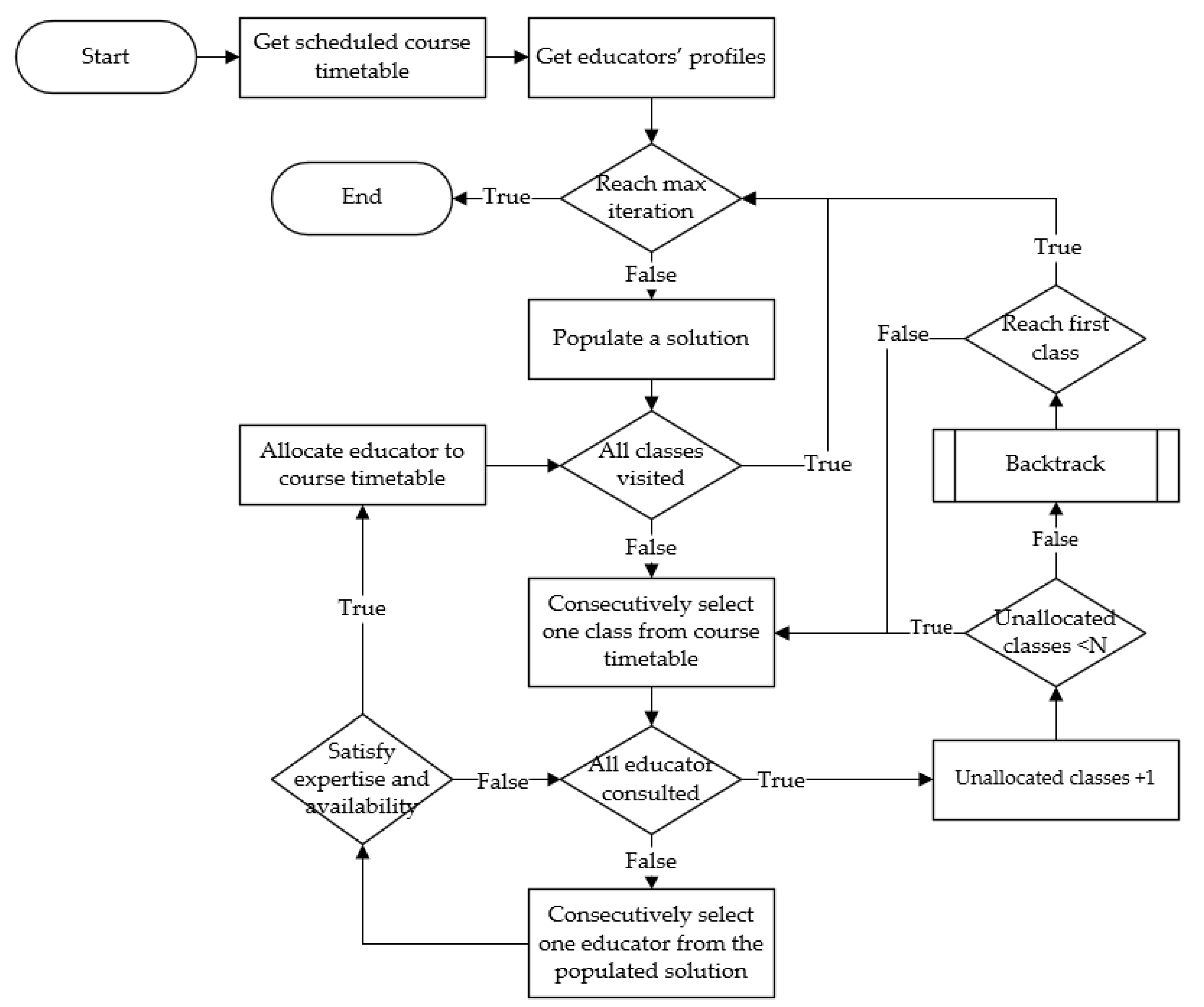
With the purpose of verifying the performance of the proposed approach in solving STPs, a CP is implemented for the comparison study, since STPs are considered constraint satisfaction problems and CP has been proven to successfully solve various problems, including timetabling [58]. The CP applied to the investigated problem is demonstrated in Figure 4. The steps of testing data retrieval and solution population are the same as the ones detailed in the initialisation stage in Step 1 of Algorithm 1. After that, unassigned classes and the populated educator list will be consecutively visited. If the consulting educator satisfies the constraints of expertise and availability of the selected class, the educator will be allocated to the class. If none of the educators can be allocated to the current class, the class will remain unassigned and the consecutive class will be selected to look for an eligible educator. If the number of unassigned classes exceeds the limitation, backtracking will be triggered. If all the classes have attempted to be assigned an educator, a solution will be outputted, and then its objective function value will be evaluated. If the backtracking reaches the first class of the course timetable, the current solution is not feasible and another solution will be populated.
To allow the modified ABC algorithm and CP be more comparative, the CP will be fed with Sample A, shown in Table 4, which can reach a better solution with the smallest population and iteration. As it is known that there are 27 unassignable classes in the dataset, to avoid over-backtracking, the compared approach sets up a backtracking trigger with the value 27, which is the N parameter in Figure 4.
This comparison study tests both the proposed modified ABC algorithm and CP ten times. The results of time spent in program execution, the number of unallocated classes and the objective function value will be compared. The comparison results are represented in Table 6.

Table 6.
Comparison results of ABC approach and CP approach.
| Items | Proposed ABC | CP | ||
|---|---|---|---|---|
| Best | Average | Best | Average | |
| Time spent (seconds) | 4.742 | 4.983 | 3.5 | 3.6108 |
| Unallocated classes 1 | 0 | 0.5 | 12 | 12 |
| Objective function values | 44.0740 | 42.4299 | 30.5128 | 30.1158 |
1 The numbers have been offset by 27. Those 27 classes have been manually confirmed as non-allocatable.
From Table 6, the following findings can be discovered.
- CP is slightly faster than the modified ABC algorithm in solution-seeking (3.6108 s over 4.983 s on average).
- The modified ABC algorithm can allocate all the non-conflict classes. However, CP has 12 allocatable classes left.
- The modified ABC algorithm can seek a solution that is 40.88% better than CP in terms of objective function values gaining (42.4299 against 30.1158 on average).
Overall, the modified ABC algorithm can find out a better solution than CP in terms of hard constraint satisfaction and objective function optimisation. Although the proposed ABC is slower than CP in program execution, a one-second time difference for a practical scenario is insignificant.
7. Conclusions and Future Work
This research aims at providing an effective solution for solving an STP with the considerations of educators’ availabilities, preferences and expertise as a whole. The STP is an ETP that has not advanced as quickly as the other two types due to its diversity and complexity. Most STP research has only focused on educators’ availabilities rather than taking educators’ preferences and expertise into consideration. This paper proposed a conceptual model of the STP and introduced a novel VSS method to reduce the searching space. A modified ABC algorithm is applied to the STP model.
The proposed approach is simulated with a large, randomly generated dataset. The experimental results demonstrate that the proposed approach is able to solve the STP and handle a large dataset in an ordinary computer hardware environment, thereby significantly reducing computational costs. Compared to the traditional constraint programming method, the proposed approach is more effective and can provide more satisfactory solutions by considering educators’ availabilities, preferences and expertise levels.
For future work, the proposed approach will be tested with datasets from real-world cases. The computing performance will be further evaluated by comparing it with other bio-inspired optimisation algorithms such as PSO.
Author Contributions
Conceptualisation, K.Z.; data curation, L.D.L.; formal analysis, K.Z.; investigation, L.D.L.; methodology, K.Z. and M.L.; project administration, L.D.L.; software, K.Z.; supervision, L.D.L. and M.L.; validation, L.D.L.; writing—original draft, K.Z.; writing—review and editing, L.D.L. and M.L. All authors have read and agreed to the published version of the manuscript.
Funding
This research received no external funding.
Institutional Review Board Statement
Not applicable.
Informed Consent Statement
Not applicable.
Data Availability Statement
The data dataset related to this research is stored in CQ University’s intranet network folder. Please contact the correspondence for the details.
Conflicts of Interest
The authors declare no conflict of interest.
References
- Wren, A. Scheduling, Timetabling and Rostering—A Special Relationship? In International Conference on the Practice and Theory of Automated Timetabling; Springer: Berlin/Heidelberg, Germany, 1995; pp. 46–75. [Google Scholar]
- Schaerf, A. A Survey of Automated Timetabling. Artif. Intell. Rev. 1999, 13, 87–127. [Google Scholar] [CrossRef]
- Valouxis, C.; Gogos, C.; Alefragis, P.; Housos, E. Decomposing the High School Timetable Problem. In Proceedings of the Practice and Theory of Automated Timetabling (PATAT 2012), Son, Norway, 29–31 August 2012. [Google Scholar]
- Bashab, A.; Ibrahim, A.O.; AbedElgabar, E.E.; Ismail, M.A.; Elsafi, A.; Ahmed, A.; Abraham, A. A Systematic Mapping Study on Solving University Timetabling Problems Using Meta-Heuristic Algorithms. Neural Comput. Appl. 2020, 32, 17397–17432. [Google Scholar] [CrossRef]
- Garey, M.R.; Johnson, D.S.; Stockmeyer, L. Some Simplified NP-Complete Problems. In Proceedings of the Sixth Annual ACM Symposium on Theory of Computing, Seattle, WA, USA, 30 April–2 May 1974; pp. 47–63. [Google Scholar]
- Odeniyi, O.; Omidiora, E.; Olabiyisi, S.; Oyeleye, C. A Mathematical Programming Model and Enhanced Simulated Annealing Algorithm for the School Timetabling Problem. Asian J. Res. Comput. Sci. 2020, 5, 21–38. [Google Scholar] [CrossRef]
- Pillay, N. A Survey of School Timetabling Research. Ann. Oper. Res. 2014, 218, 261–293. [Google Scholar] [CrossRef]
- Beligiannis, G.N.; Moschopoulos, C.N.; Kaperonis, G.P.; Likothanassis, S.D. Applying Evolutionary Computation to the School Timetabling Problem: The Greek Case. Comput. Oper. Res. 2008, 35, 1265–1280. [Google Scholar] [CrossRef]
- Post, G.; Ahmadi, S.; Daskalaki, S.; Kingston, J.H.; Kyngas, J.; Nurmi, C.; Ranson, D.; Ruizenaar, H. An XML Format for Benchmarks in High School Timetabling. Ann. Oper. Res. 2012, 194, 385–397. [Google Scholar] [CrossRef] [Green Version]
- Wilke, P.; Ostler, J. Solving the School Time Tabling Problem Using Tabu Search, Simulated Annealing, Genetic and Branch & Bound Algorithms. In Proceedings of the 7th International Conference on the Practice and Theory of Automated Timetabling (PATAT 2008), Montreal, Canada, 19–22 August 2008. [Google Scholar]
- Babaei, H.; Karimpour, J.; Hadidi, A. A Survey of Approaches for University Course Timetabling Problem. Comput. Ind. Eng. 2015, 86, 43–59. [Google Scholar] [CrossRef]
- Feizi-Derakhshi, M.-R.; Babaei, H.; Heidarzadeh, J. A Survey of Approaches for University Course Timetabling Problem. In Proceedings of the 8th International Symposium on Intelligent and Manufacturing Systems, Adrasan, Turkey, 27–28 September 2012; Sakarya University Department of Industrial Engineering: Adrasan, Turkey, 2012; pp. 307–321. [Google Scholar]
- Salhi, S. Heuristic Search: The Emerging Science of Problem Solving; Springer: Berlin/Heidelberg, Germany, 2017. [Google Scholar]
- Fonseca, G.H.; Santos, H.G.; Carrano, E.G.; Stidsen, T.J. Integer Programming Techniques for Educational Timetabling. Eur. J. Oper. Res. 2017, 262, 28–39. [Google Scholar] [CrossRef] [Green Version]
- Pillay, N.; Qu, R. Hyper-Heuristics: Theory and Applications; Springer: Berlin/Heidelberg, Germany, 2018. [Google Scholar]
- Fong, C.W.; Asmuni, H.; McCollum, B. A Hybrid Swarm-Based Approach to University Timetabling. IEEE Trans. Evolut. Comput. 2015, 19, 870–884. [Google Scholar] [CrossRef]
- Ishak, S.; Lee, L.S.; Ibragimov, G. Hybrid Genetic Algorithm for University Examination Timetabling Problem. Malays. J. Math. Sci. 2016, 10, 145–178. [Google Scholar]
- Kouhbanani Nejad, S.F.; Farid, D.; Sadeghi, H. Selection of Optimal Portfolio Using Expert System in Mamdani Fuzzy Environment. Ind. Manag. Stud. 2018, 16, 131–151. [Google Scholar]
- Bělohlávek, R.; Dauben, J.W.; Klir, G.J. Fuzzy Logic and Mathematics: A Historical Perspective; Oxford University Press: Oxford, UK, 2017. [Google Scholar]
- Junn, K.Y.; Obit, J.H.; Alfred, R.; Bolongkikit, J. A Formal Model of Multi-agent System for University Course Timetabling Problems; Springer: Singapore, 2019; pp. 215–225. [Google Scholar]
- Odeniyi, O.; Omidiora, E.; Olabiyisi, S.; Aluko, J. Development of a Modified Simulated Annealing to School Timetabling Problem. Int. J. Appl. Inf. Syst. 2015, 8, 16–24. [Google Scholar] [CrossRef]
- Sutar, S.R.; Bichkar, R.S. Genetic Algorithms Based Timetabling Using Knowledge Augmented Operators. Int. J. Comput. Sci. Inf. Secur. 2016, 14, 570. [Google Scholar]
- Ahmed, L.N.; Özcan, E.; Kheiri, A. Solving High School Timetabling Problems Worldwide Using Selection Hyper-Heuristics. Expert Syst. Appl. 2015, 42, 5463–5471. [Google Scholar] [CrossRef] [Green Version]
- Domrös, J.; Homberger, J. An Evolutionary Algorithm for High School Timetabling. In Proceedings of the Ninth International Conference on the Practice and Theory of Automated Timetabling (PATAT 2012), Son, Norway, 29–31 August 2012. [Google Scholar]
- Sørensen, M.; Stidsen, T.R. High School Timetabling: Modeling and Solving a Large Number of Cases in Denmark. In Proceedings of the Ninth International Conference on the Practice and Theory of Automated Timetabling (PATAT 2012), Son, Norway, 29–31 August 2012; pp. 359–364. [Google Scholar]
- Fonseca, G.H.; Santos, H.G.; Carrano, E.G. Late Acceptance Hill-Climbing for High School Timetabling. J. Sched. 2016, 19, 453–465. [Google Scholar] [CrossRef]
- Skoullis, V.I.; Tassopoulos, I.X.; Beligiannis, G.N. Solving the High School Timetabling Problem Using a Hybrid Cat Swarm Optimization Based Algorithm. Appl. Soft Comput. 2017, 52, 277–289. [Google Scholar] [CrossRef]
- Katsaragakis, I.V.; Tassopoulos, I.X.; Beligiannis, G.N. A Comparative Study of Modern Heuristics on the School Timetabling Problem. Algorithms 2015, 8, 723–742. [Google Scholar] [CrossRef] [Green Version]
- Babaei, H.; Karimpour, J.; Oroji, H. Using Fuzzy C-Means Clustering Algorithm for Common Lecturers Timetabling among Departments. In Proceedings of the 2016 6th International Conference on Computer and Knowledge Engineering (ICCKE), Mashhad, Iran , 20–20 October 2016; IEEE: Manhattan, NY, USA, 2016; pp. 243–250. [Google Scholar]
- Oprea, M. MAS_UP-UCT: A Multi-Agent System for University Course Timetable Scheduling. Int. J. Comput. Commun. Control 2007, 2, 94–102. [Google Scholar] [CrossRef] [Green Version]
- Tkaczyk, R.; Ganzha, M.; Paprzycki, M. AgentPlanner-Agent-Based Timetabling System. Informatica 2016, 40, 3–17. [Google Scholar]
- Tan, J.S.; Goh, S.L.; Kendall, G.; Sabar, N.R. A Survey of the State-of-the-Art of Optimisation Methodologies in School Timetabling Problems. Expert Syst. Appl. 2021, 165, 113943. [Google Scholar] [CrossRef]
- Karaboga, D.; Gorkemli, B.; Ozturk, C.; Karaboga, N. A Comprehensive Survey: Artificial Bee Colony (ABC) Algorithm and Applications. Artif. Intell. Rev. 2014, 42, 21–57. [Google Scholar] [CrossRef]
- Bolaji, A.L.A.; Khader, A.T.; Al-Betar, M.A.; Awadallah, M.A. University Course Timetabling Using Hybridized Artificial Bee Colony with Hill Climbing Optimizer. J. Comput. Sci. 2014, 5, 809–818. [Google Scholar] [CrossRef]
- Bolaji, A.L.A.; Khader, A.T.; Al-Betar, M.A.; Awadallah, M.A. A Hybrid Nature-Inspired Artificial Bee Colony Algorithm for Uncapacitated Examination Timetabling Problems. J. Intell. Syst. 2015, 24, 37–54. [Google Scholar] [CrossRef]
- Alzaqebah, M.; Abdullah, S. Hybrid Bee Colony Optimization for Examination Timetabling Problems. Comput. Oper. Res. 2015, 54, 142–154. [Google Scholar] [CrossRef]
- Zhu, K.; Li, L.D.; Li, M. A Survey of Computational Intelligence in Educational Timetabling. IJMLC 2021, 11, 40–47. [Google Scholar] [CrossRef]
- Kristiansen, S.; Stidsen, T.R. A Comprehensive Study of Educational Timetabling—A Survey; DTU Management Engineering Report; Department of Management Engineering, Technical University of Denmark: Lyngby, Denmark, 2013. [Google Scholar]
- Chen, M.C.; Goh, S.L.; Sabar, N.R.; Kendall, G. A Survey of University Course Timetabling Problem. Perspect. Trends Oppor. IEEE Access. 2021, 9, 106515–106529. [Google Scholar] [CrossRef]
- Mirjalili, S.; Lewis, A. The Whale Optimization Algorithm. Adv. Eng. Softw. 2016, 95, 51–67. [Google Scholar] [CrossRef]
- Adrianto, D. Comparison Using Particle Swarm Optimization and Genetic Algorithm for Timetable Scheduling. J. Comput. Sci. 2014, 10, 341. [Google Scholar] [CrossRef] [Green Version]
- Kennedy, J.; Eberhart, R. Particle Swarm Optimization. In Proceedings of the ICNN’95-International Conference on Neural Networks, Perth, WA, Australia, 27 November–1 December 1995; IEEE: Manhattan, NY, USA, 1995; pp. 1942–1948. [Google Scholar]
- Patrick, K.; Godswill, Z. Greedy Ants Colony Optimization Strategy for Solving the Curriculum Based University Course Timetabling Problem. J. Adv. Math. Comput. Sci. 2016, 14, 1–10. [Google Scholar] [CrossRef]
- Neshat, M.; Sepidnam, G.; Sargolzaei, M.; Toosi, A.N. Artificial Fish Swarm Algorithm: A Survey of the State-of-the-Art, Hybridization, Combinatorial and Indicative Applications. Artif. Intell. Rev. 2014, 42, 965–997. [Google Scholar] [CrossRef]
- Yang, X.-S. Firefly Algorithms for Multimodal Optimization. International Symposium on Stochastic Algorithms; Springer: Berlin/Heidelberg, Germany, 2009; pp. 169–178. [Google Scholar]
- Eusuff, M.M.; Lansey, K.E. Optimization of Water Distribution Network Design Using the Shuffled Frog Leaping Algorithm. J. Water Resour. Plan. Manag. 2003, 129, 210–225. [Google Scholar] [CrossRef]
- Clerc, M.; Kennedy, J. The Particle Swarm-Explosion, Stability, and Convergence in a Multidimensional Complex Space. IEEE Trans. Evolut. Comput. 2002, 6, 58–73. [Google Scholar] [CrossRef] [Green Version]
- Dorigo, M.; Birattari, M. Swarm Intelligence. Scholarpedia 2007, 2, 1462. [Google Scholar] [CrossRef]
- Ilyas, R.; Iqbal, Z. Study of Hybrid Approaches Used for University Course Timetable Problem (UCTP). In Proceedings of the 2015 IEEE 10th Conference on Industrial Electronics and Applications (ICIEA), Auckland, New Zealand, 15–17 June 2015; IEEE: Manhattan, NY, USA, 2015; pp. 696–701. [Google Scholar]
- Oner, A.; Ozcan, S.; Dengi, D. Optimization of University Course Scheduling Problem with a Hybrid Artificial Bee Colony Algorithm. In Proceedings of the 2011 IEEE Congress of Evolutionary Computation (CEC), New Orleans, LA, USA, 5–8 June 2011; IEEE: Manhattan, NY, USA, 2011; pp. 339–346. [Google Scholar]
- Alzaqebah, M.; Abdullah, S. An Adaptive Artificial Bee Colony and Late-Acceptance Hill-Climbing Algorithm for Examination Timetabling. J. Sched. 2014, 17, 249–262. [Google Scholar] [CrossRef]
- Karaboga, D. An Idea Based on Honey Bee Swarm for Numerical Optimization; Technical Report-TR06; Erciyes University: Kayseri, Turkey, 2005. [Google Scholar]
- Veček, N.; Mernik, M.; Filipič, B.; Črepinšek, M. Parameter Tuning with Chess Rating System (CRS-Tuning) for Meta-Heuristic Algorithms. Inf. Sci. 2016, 372, 446–469. [Google Scholar] [CrossRef]
- Ma, M.; Liang, J.; Guo, M.; Fan, Y.; Yin, Y. SAR Image Segmentation Based on Artificial Bee Colony Algorithm. Appl. Soft Comput. 2011, 11, 5205–5214. [Google Scholar] [CrossRef]
- Zhang, C.; Ouyang, D.; Ning, J. An Artificial Bee Colony Approach for Clustering. Expert Syst. Appl. 2010, 37, 4761–4767. [Google Scholar] [CrossRef]
- Xu, C.; Duan, H.; Liu, F. Chaotic Artificial Bee Colony Approach to Uninhabited Combat Air Vehicle (UCAV) Path Planning. Aerosp. Sci.Technol. 2010, 14, 535–541. [Google Scholar] [CrossRef]
- Samanta, S.; Chakraborty, S. Parametric Optimization of Some Non-Traditional Machining Processes Using Artificial Bee Colony Algorithm. Eng. Appl. Artif. Intell. 2011, 24, 946–957. [Google Scholar] [CrossRef]
- Bukchin, Y.; Raviv, T. Constraint Programming for Solving Various Assembly Line Balancing Problems. Omega 2018, 78, 57–68. [Google Scholar] [CrossRef]
Figure 1.
School timetabling concept model.

Figure 2.
Bipartite graph for the STP.

Figure 3.
Concept of allocating educators to units.

Figure 4.
Constraint programming flowchart.

Table 1.
Example of preference and expertise table.
| Class ID | Preference | Expertise |
|---|---|---|
| 2 | 3 | |
| 1 | 1 | |
| … | … | … |
| 3 | 2 | |
| … | … | … |
| 0 | 0 |
Table 2.
Example of educator’s availability.
| Mon | Tue | Wed | Thu | Fri | |
|---|---|---|---|---|---|
| 8:00 a.m. | Y | N | Y | N | N |
| 9:00 a.m. | Y | N | N | N | N |
| 10:00 a.m. | Y | Y | N | N | N |
| 11:00 a.m. | Y | Y | Y | N | N |
| 12:00 p.m. | N | Y | Y | N | N |
| 1:00 p.m. | N | N | Y | N | Y |
| 2:00 p.m. | N | N | Y | N | Y |
| 3:00 p.m. | N | Y | Y | N | Y |
| 4:00 p.m. | N | N | Y | N | Y |
| 5:00 p.m. | Y | N | Y | N | Y |
| 6:00 p.m. | Y | N | Y | N | Y |
Note: Y means available, N means unavailable. This table will be converted to be a one-dimensional array. The total number of cells in the array equals to the multiplication of . The index 1 refers to the first timeslot of the first day. The index indicates the last timeslot of the last day.
Table 3.
Example of searching space.
| A region | B region | ||||||||||
| 1 | 2 | 3 | 4 | 5 | 6 | 7 | 8 | 9 | 10 | 11 | 12 |
| A | A | A | A | A | A | B | B | B | B | B | B |
| B | B | C | C | D | D | A | A | C | C | D | D |
| C | D | B | D | B | C | C | D | A | D | A | C |
| D | C | D | B | C | B | D | C | D | A | C | A |
| C region | D region | ||||||||||
| 13 | 14 | 15 | 16 | 17 | 18 | 19 | 20 | 21 | 22 | 23 | 24 |
| C | C | C | C | C | C | D | D | D | D | D | D |
| A | A | B | B | D | D | A | A | B | B | C | C |
| B | D | A | D | A | B | B | C | A | C | A | B |
| D | B | D | A | B | A | C | B | C | A | B | A |
Table 4.
Parameter settings for modified ABC algorithm.
| Sample | Num of Bees | Neighbour Range | Num of Iterations | Num of Traits |
|---|---|---|---|---|
| A | 5 | 5 | 1000 | 10 |
| B | 20 | 5 | 1000 | 10 |
| C | 5 | 30 | 1000 | 10 |
| D | 5 | 5 | 10,000 | 10 |
| E | 5 | 5 | 1000 | 30 |
| F | 20 | 30 | 10,000 | 10 |
| G | 20 | 30 | 10,000 | 30 |
| H | 5 | 5 | 10,000 | 30 |
| I | 20 | 30 | 10,000 | 30 |
| J | 40 | 60 | 20,000 | 60 |
Table 5.
Experiment result (run ten times).
| Sample | Objective Values | Time Spent (Seconds) | Unallocated Classes | |||||||
|---|---|---|---|---|---|---|---|---|---|---|
| Avg. | Best | Std. Dev. | CV | Avg. | Best | Std. Dev. | CV | Avg 1 | Best | |
| A | 42.4299 | 44.0740 | 0.9697 | 2.285% | 4.983 | 4.742 | 0.2712 | 5.443% | 0.5 | 0 |
| B | 43.4970 | 44.7037 | 0.6937 | 1.594% | 18.8521 | 18.453 | 0.4208 | 2.232% | 0.1 | 0 |
| C | 42.7910 | 43.7407 | 0.6779 | 1.584% | 5.0719 | 4.834 | 0.1950 | 3.846% | 0.5 | 0 |
| D | 43.6596 | 44.8518 | 0.6690 | 1.532% | 48.843 | 47.238 | 2.4431 | 5.002% | 0 | 0 |
| E | 41.9709 | 43.9256 | 1.0925 | 2.603% | 4.9919 | 4.818 | 0.1732 | 3.470% | 1 | 0 |
| F | 44.7148 | 45.3703 | 0.4201 | 0.939% | 197.513 | 193.957 | 2.2012 | 1.114% | 0 | 0 |
| G | 44.5255 | 45.1481 | 0.2849 | 0.639% | 201.0127 | 194.826 | 6.5969 | 3.281% | 0 | 0 |
| H | 42.5502 | 43.2222 | 0.4757 | 1.118% | 50.3867 | 46.775 | 3.9439 | 7.827% | 0.3 | 0 |
| I | 44.4592 | 45.8148 | 0.5484 | 1.228% | 206.4878 | 197.141 | 7.1228 | 3.449% | 0 | 0 |
| J | 46.8359 | 47.1481 | 0.2448 | 0.522% | 831.6302 | 813.494 | 441.1553 | 4.467% | 0 | 0 |
1 The numbers have been offset by 27. Those 27 classes have been manually confirmed as non-allocatable.
Publisher’s Note: MDPI stays neutral with regard to jurisdictional claims in published maps and institutional affiliations. |
© 2021 by the authors. Licensee MDPI, Basel, Switzerland. This article is an open access article distributed under the terms and conditions of the Creative Commons Attribution (CC BY) license (https://creativecommons.org/licenses/by/4.0/).
Share and Cite
MDPI and ACS Style
Zhu, K.; Li, L.D.; Li, M. School Timetabling Optimisation Using Artificial Bee Colony Algorithm Based on a Virtual Searching Space Method. Mathematics 2022, 10, 73. https://0-doi-org.brum.beds.ac.uk/10.3390/math10010073
AMA Style
Zhu K, Li LD, Li M. School Timetabling Optimisation Using Artificial Bee Colony Algorithm Based on a Virtual Searching Space Method. Mathematics. 2022; 10(1):73. https://0-doi-org.brum.beds.ac.uk/10.3390/math10010073
Chicago/Turabian StyleZhu, Kaixiang, Lily D. Li, and Michael Li. 2022. "School Timetabling Optimisation Using Artificial Bee Colony Algorithm Based on a Virtual Searching Space Method" Mathematics 10, no. 1: 73. https://0-doi-org.brum.beds.ac.uk/10.3390/math10010073
Note that from the first issue of 2016, this journal uses article numbers instead of page numbers. See further details here.