Estimation of Linear Regression with the Dimensional Analysis Method

Abstract

Dimensional Analysis (DA) is a mathematical method that manipulates the data to be analyzed in a homogenized manner. Likewise, linear regression is a potent method for analyzing data in diverse fields. At the same time, data visualization has gained attention in tendency study. In addition, linear regression is an important topic to address predictive models and patterns in data study. However, it is still pending to attack the manipulation of uncertainty related to the data transformation. In this sense, this work presents a new contribution with linear regression, combining the Dimensional Analysis (DA) to address instability and error issues. In addition, our method provides a second contribution related to including the decision maker’s attitude involved in the study. Therefore, the experimentation shows that DA manipulates the regression problem under a complex situation that the outcome may have in the investigation. A real-life case study is used to demonstrate our proposal.

1. Introduction

Linear regression (LR) model utilized in numerous areas of application [1]: for example, engineering, economics, ecological, social sciences, and medicines, among many others. Hence, linear regression is a potent and flexible technique in order to address regression issues. Thus, the trend of LR model is an extensive topic with important interest for researchers according [2,3,4].

Moreover, according to [5,6,7], the topic related to inventories play a key role because represent around 60% about operational cost for the organizations. Generally, the inventories are classified as following: (1) raw material, (2) work in process, (3) spare parts, and (4) finish good, etc. In addition, the interest related to inventory is due to cost management strategies by organizations [8,9,10,11]. Based on operation research, the inventories can be used in order to addressed considerable reduction cost. Therefore, the forecast method is imperative in order to determine the quantities with accuracy avoiding minimal error [12]. In this mode, the literature review explains the use of several methods focused to forecast of the inventories: for example, Linear regression and time series [13,14], Neural Networks [11,15], Machine Learning [16], and Bayesian principal component regression model [17], among others [10,18].

Additionally, dimensional analysis (DA) presents extensive interest in engineering [19,20]. DA has the potential to model, simplification the scale and dimension of the variable [21]. Thus, applications of neural networks [22], Matrix manipulations [23], physical sciences applications [24], revolutionary dimensional analysis methods [25,26], and statistical theories for dimensional analysis [27].

Therefore, dimensional analysis (DA) is a proficient tool that involves the interrelationship of the data or arguments under analysis. Much different research on DA is related to the statistical situation [28,29,30,31]. In this mode, Dovi [32], reported the improving the statistical accuracy of dimensional analysis correlations. However, this work does not consider the attitude of the decisors.

The literature reveal a substantial interest in dealing with the next crucial gaps:

• The vital element is the instability of the prediction method [33,34];
• Minimize the median squared difference between observed and fitted response [35];
• Verify the efficacy of the algorithm, the greatest robustness, and accuracy in forecast results [12,36,37,38,39,40,41].

Based on the aforementioned considerations, the concrete contributions of this paper are the following:

• We formulate a method to attack the drawbacks related to efficiency, instability, and minimal error.
• This study explores the significant application of linear regression model under Dimensional Analysis.
• The novelty of the current study also lies in considering the grade of importance of the decision makers or experts involved implied to solve the problem.
• Finally, the proposed includes an application of DA to linear regression to deal with an inventory forecast problem.

The remainder of this paper is structured as follows: Section 2 presents basic concepts. The research methodology is described in Section 3. A numerical case study is presented in Section 4. Section 5 provides the discussions of findings. Finally, the conclusion is given in Section 6.

2. Basic Concepts

This section introduces the basic concepts used in this document.

2.1. Linear Regression

The linear regression (LR) method used to approximate a pendent variable reported to the values or changes of other variables studied in a linear shape.

Definition 1.

Let $x_i$ and $y_i$ be two variables within a random and continued distribution. In this mode, assuming a numerical data set mapped by $(x_i,y_i)$ for $i=1,2,\cdots ,n$, where $x_i\in U^n$ and $y_i\in U^n$. A reasonable form of relation between the response variable called Y and the regressor X is the linear relationship. In this manner, a model can be represented as follows, where ${\ddot{Y}}_l$ of dimension n is a mapping in space $R^n\to R$, captured by a vector of analysis related to metrics involved, and ${\rm Y}\in \omega \subseteq R^P$, which is built by χ and Γ; In this mode, the simple linear regression depicted by means of Equation (1):

$${\ddot{Y}}_l=\chi +\Gamma X_l$$

(1)

where χ is the value stand for the value of when $X_l=0$, also called the intersection, and Γ is the change in ${\ddot{Y}}_l$ called the slope of the line.

2.2. Dimensional Analysis

The mathematical expresion of DA is depicted by Equation (2) as follows:

$$DA=\prod _{i=1}^n{\left(\frac{x_i}{S_i}\right)}^{{\tau }_i}.$$

(2)

where:

$x_i=$ is the numerical argument for $i=1,2,\cdots ,n$;

$S_i=$ is the best numerical datum taken from the data set under analysis;

${\tau }_i=$ is the grade of altitude or weight of the decision (expert) within a vector.

In this sense, the parameter ${\tau }_j$ for $j=1,2,\cdots ,m$ and $\tau \in \left[0,1\right].$

Definition 2.

In this mode can be introduced the mean for $x_i$ based on the Equation (3). Considering $x_i$, a numerical data set of $R^n\to R$ that maintains random conditions and continue distribution is created:

$$mea{n}_{DA}=\prod _{i=1}^n{\left(\frac{x_i}{S_i}\right)}^{{\tau }_j}$$

(3)

The solution in terms of the original argument is obtained by substituting ${\prod }_{i=1}^n{\left(\frac{x_i}{y_i}\right)}^{{\tau }_j}$:

$$\begin{array}{cc}mea{n}_{DA}\hfill & ={\sum }_{i=1}^n〈\prod _{i=1}^n{\left(\frac{x_i}{S_i}\right)}^{{\tau }_j}〉\hfill \\ \hfill & ={\sum }_{i=1}^n〈{\left(\frac{x_1}{S_1}\right)}^{{\tau }_1}\times {\left(\frac{x_2}{S_2}\right)}^{{\tau }_2}\times ,\cdots ,\times {\left(\frac{x_n}{S_n}\right)}^{{\tau }_m}〉,\hfill \end{array}$$

(4)

then:

$$mea{n}_{DA}=\sum _{i=1}^n〈\prod _{i=1}^n{\left(\frac{x_i}{S_i}\right)}^{{\tau }_j}〉.$$

(5)

Example 1.

Assuming a set called $a_1=\left(2,3,6,7\right)$, it will receive a vector weight $\tau =\left(0.25,0.25,0.25,0.25\right)$ and has been determined to be $S_i=\left(4.5\right)$. Then, applying Equation (5), we will obtain the $mea{n}_{DA}$ result for this example:

$$mea{n}_{DA}={\sum }_{i=1}^4〈{\left(\frac{2}{4.5}\right)}^{0.25}\times {\left(\frac{3}{4.5}\right)}^{0.25}\times {\left(\frac{6}{4.5}\right)}^{0.25}\times {\left(\frac{7}{4.5}\right)}^{0.25}〉=3.911.$$

3. Main Results

In this section, we present the generalized linear regression method under the Dimensional Analysis environment.

3.1. Generalized Linear Regression Method under Dimensional Analysis Environment

This section presents a generalized linear regression method under the Dimensional Analysis environment called (GLR-DA):

$$\ddot{Y}=\gamma +{\beta }_{DA}x.$$

(6)

Let A be the mean of x, and let $x_s$ depict the ideal value of x under dimensional analysis. Then:

$$A=\prod _{i=1}^n{\left(\frac{x_i}{x_s}\right)}^{{\tau }_j}.$$

(7)

B represents y, and $y_s$ depicts the ideal value of y under dimensional analysis. Then:

$$B=\prod _{i=1}^n{\left(\frac{y_i}{y_s}\right)}^{{\tau }_j}.$$

(8)

$$\ddot{Y}=\gamma +{\beta }_{DA}x+D_i.$$

(9)

where $\ddot{Y}$ is a vector of responses; $\gamma$ is a normally scattered vector of random data obtaining the expected value $=0$, also called the intersection; ${\beta }_{DA}$ is the weight vector corresponding to x; and x is the full rank matrix of not random variables.

3.2. Compute the Mean and Variance Estimators

The estimated values of the parameters $\gamma$ and ${\beta }_{DA}$ given in the regression line (9) are found by using the method of the least-squares and get

$$\gamma =\frac{{\sum }_{z=1}^Z{y}_z-{\beta }_{DA}\left({\sum }_{z=1}^Z{x}_z\right)}{n}=\overline{y}-{\beta }_{DA}\overline{x}$$

(10)

$${\beta }_{DA}=\frac{{\sum }_{z=1}^Z\left(x_z-A\right)\left(y_z-B\right)}{{\sum }_{i=1}^k{\left(x_z-A\right)}^2}$$

(11)

In addition to the assumptions that the error D in the model is a random variable with mean $\lambda =0$ and variance ${\theta }^2$ constant, also suppose that $D_1,D_2,\cdots ,D_n$ are independent from one run of the experiment to another. In this sense, under random conditions, the mean $\lambda$ presented in Equation (12) and the variance ${\theta }^2$ in Equation (14) can be obtained as follows: In Figure 1 depict the random conditions for error D.

Thus, the mathematical expectation is:

$$E(\lambda -{\lambda }_x)=E\left(\lambda \right)-E\left({\lambda }_x\right)=0$$

(12)

The covariance ${\widehat{S}}_{xy}$ is depicted as follows:

$${\widehat{S}}_{xy}={\displaystyle \frac{1}{Z}}\sum _{z=1}^Z\left(x_z-A\right)\left(y_z-B\right)$$

(13)

where:

$$A={\displaystyle \frac{1}{Z}}\sum _{z=1}^Z{x}_z,andB={\displaystyle \frac{1}{Z}}\sum _{z=1}^Z{y}_z$$

To determine related bias information, it is imperative obtain the variance. In this sense, it is possible to carry out a modelization of error called $\xi$:

$$E\left(S^2\right)={\theta }^2={\displaystyle \frac{1}{n-2}}\sum _{z=1}^Z\left(x_z-A\right)\left(y_z-B\right)$$

(14)

Thus, the difference between observations $x_i$ and estimated value of $A={\displaystyle \frac{1}{Z}}\sum _{z=1}^Z{x}_z$ is given as:

$${\xi }_t=\sum _{z=1}^Z{\left(x_z-A\right)}^2,$$

(15)

Moreover, the difference between observations $y_i$ and estimated value of $B={\displaystyle \frac{1}{Z}}\sum _{z=1}^Z{y}_z$ is given as:

$${\xi }_s=\sum _{z=1}^Z{\left(y_z-B\right)}^2,$$

(16)

and the aggregation error of $x_i$ and $y_i$, respectively, converge in the Equation (17):

$$\widehat{S}=\sum _{z=1}^Z\left(x_z-A\right)\left(y_z-B\right).$$

(17)

In addition, the sum of the squares of the error can be presented as follows:

$$SSE=\sum _{z=1}^Z{\xi }^2=\sum _{z=1}^Z{\left(y_z-\gamma -{\beta }_{DA}{x}_z\right)}^2$$

(18)

Then, assuming that ${\beta }_{DA}=\frac{\widehat{S}}{{\xi }_t}$, the solution for Equation (18) and using Equations (14)–(16) can be obtained as follows:

$$SSE=\sum _{z=1}^Z{\left(\left(y_z-B\right)-{\beta }_{DA}\left(x_z-A\right)\right)}^2$$

$$=\sum _{z=1}^k{\left(y_z-\gamma \right)}^2-2{\beta }_{DA}\sum _{z=1}^Z\left(y_z-B\right)\left(x_z-A\right)+{\beta }_{DA}^2\sum _{z=1}^Z{\left(x_z-A\right)}^2$$

$$={\xi }_s-2{\beta }_{DA}\left(\widehat{S}\right)+{\beta }_{DA}^2{\xi }_t$$

$$={\xi }_s-2\left(\frac{\widehat{S}}{{\xi }_t}\right)\left(\widehat{S}\right)+{\left(\frac{\widehat{S}}{{\xi }_t}\right)}^2{\xi }_t$$

$$={\xi }_s-2\left(\frac{{\widehat{S}}^2}{{\xi }_t}\right)+\left(\frac{{\widehat{S}}^2}{{\xi }_t^2}{\xi }_t\right)$$

$$={\xi }_s-2\left(\frac{{\widehat{S}}^2}{{\xi }_t}\right)+\left(\frac{{\widehat{S}}^2{\xi }_t}{{\xi }_t^2}\right)$$

Finally:

$$SSE={\xi }_s-\left(\frac{{\widehat{S}}^2}{{\xi }_t}\right)={\xi }_s-\left(\frac{\widehat{S}}{{\xi }_t}\right)\widehat{S}$$

Then, the sum of the squares of the error (SSE) is depicted as follows:

$$SSE={\xi }_s-\left({\beta }_{DA}\right)\widehat{S}$$

(19)

Additionally, an unbiased estimator of the mean square error (MSE) is:

$$S^2=\frac{{\xi }_s-\left({\beta }_{D{A}_1}\right)\widehat{S}}{n-2}=\frac{SSE}{n-2}=MSE$$

(20)

4. Numerical Example

In this section, two numerical cases are presented to demonstrate our proposal.

4.1. Numerical Example from a Real Case Study

A real case is considered in a manufacturing company’s need to establish a forecast related to inventory handling. This company is facing problems related to the forecast accuracy of raw material. In this mode, the data set used in this study will be under an inventory prediction problem. Our proposed GLR-DA will addressing a inventory problem to estimate the inventory conditions. The data considered are depicted in

Table 1. Numerical data.

x	y	x	y
1	32	7	89
2	40	8	94
3	40	9	96
4	45	10	96
5	64	11	121
6	71	12	125

.

The approach requires a pairwise comparison of the variables x and y based on the following model according Equation (5). In

Table 2. Estimation of the parameters A and B.

A	B
0.11	5.63142487
0.14	4.45475331
0.19	3.63920858
0.21	3.34356494
0.26	3.56587087
0.22	3.42892914
0.19	3.55394256
0.35	3.4168655
0.35	3.25595148
0.41	3.0892899
0.43	3.30630209
0.46	3.21766878
mean 3.32	mean 43.903772

, the results obtained for each parameter A and B are depicted.

The following results applying our method proposed are depicted in

Table 3. Details and error study.

Real	Prediction	${\mathbf{Case}}_{\mathit{M}}$	${\mathit{\xi }}_{\mathit{s}}$	$|{\mathit{\xi }}_{\mathit{s}}|$	${\mathit{\xi }}_{\mathit{s}}^2$
32.00	20.50	27.9	11.5	11.5	132.2
40.00	30.61	36.6	9.4	9.4	88.2
40.00	40.71	45.4	−0.7	0.7	0.5
45.00	50.81	54.2	−5.8	5.8	33.8
64.00	60.92	62.9	3.1	3.1	9.5
71.00	71.02	71.7	−0.0	0.0	0.0
89.00	81.12	80.5	7.9	7.9	62.0
94.00	91.23	89.2	2.8	2.8	7.7
96.00	101.33	98.0	−5.3	5.3	28.4
96.00	111.43	106.8	−15.4	15.4	238.2
121.00	121.54	115.5	−0.5	0.5	0.3
125.00	131.64	124.3	−6.6	6.6	44.1
		Total	0.14	69.11	644.97
		Average	0.01	5.76	53.75

.

Hence, the SME is obtained using Equation (20):

$$\begin{array}{c}\hfill MSE={\displaystyle \frac{644.97}{10}}=64.44\end{array}$$

The Pearson correlation [42] is presented in

Table 4. Correlation matrix.

	Real Data	Prediction with GLR-DA	Conventional Regression
Real Data	1.0000000	0.9827522	0.9827528
Prediction with GLR-DA	0.9827522	1.0000000	1.0000000
Conventional regression	0.9827528	1.0000000	1.0000000

, where a strong correlation between the information for each variable is observed.

Finally, it is important to consider that the correlation coefficient is around to 98.27%. It is a strong value to confirm that the forecast obtained with our proposal is proficient and robust.

4.2. Numerical Example 2

The data for this experiment were taken from [43] focused on a sales estimation study. In this mode, the data are presented in

Table 5. Sales data by weeks.

x	y
1	9
2	8
3	10
4	10
5	10
6	8
7	7
8	10
9	8
10	10
11	10
12	9
13	9

, and for convenience, x represents the weeks and y describes the sales.

According to the results represents in

Table 6. Details of the estimations.

Real	Prediction	${\mathit{\xi }}_{\mathit{s}}$	$|{\mathit{\xi }}_{\mathit{s}}|$	${\mathit{\xi }}_{\mathit{s}}^2$
9.00	2.34	6.7	6.7	44.4
8.00	3.22	4.8	4.8	22.9
10.00	4.10	5.9	5.9	34.8
10.00	4.98	5.0	5.0	25.2
10.00	5.86	4.1	4.1	17.1
8.00	6.74	1.3	1.3	1.6
7.00	7.62	−0.6	0.6	0.4
10.00	8.50	1.5	1.5	2.2
8.00	9.38	−1.4	1.4	1.9
10.00	10.27	−0.3	0.3	0.1
10.00	11.15	−1.1	1.1	1.3
9.00	12.03	−3.0	3.0	9.2
9.00	12.91	−3.9	3.9	15.3
	Total	18.90	39.62	176.40
	Average	1.90	2.98	13.43

, it can be see that our proposal has the potential to handle sales estimation problems.

In addition, the SME is obtained using Equation (20):

$$\begin{array}{c}\hfill MSE={\displaystyle \frac{176.40}{10}}=17.64\end{array}$$

5. Validations

In this section, statistical tests such as the normal probability test, correlation, means, standard deviation, confidence interval, and Tukey’s test were used. We conducted the statistical tests in order to evaluate the methodology proposal as followings.

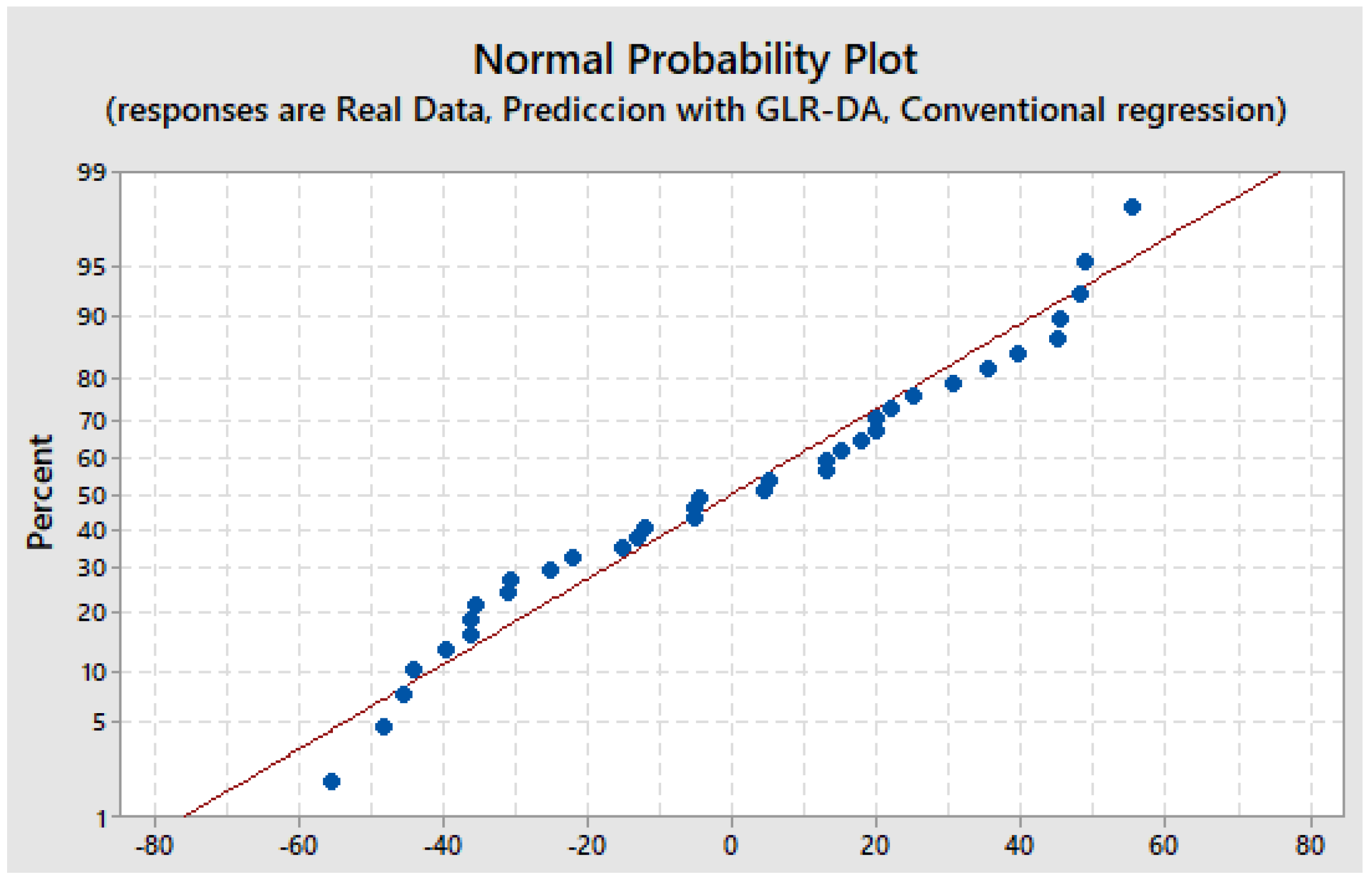
In this manner, the normal probability test is realized to appraisal the data distribution. It can be observed in Figure 2 that the normal test results are consistent.

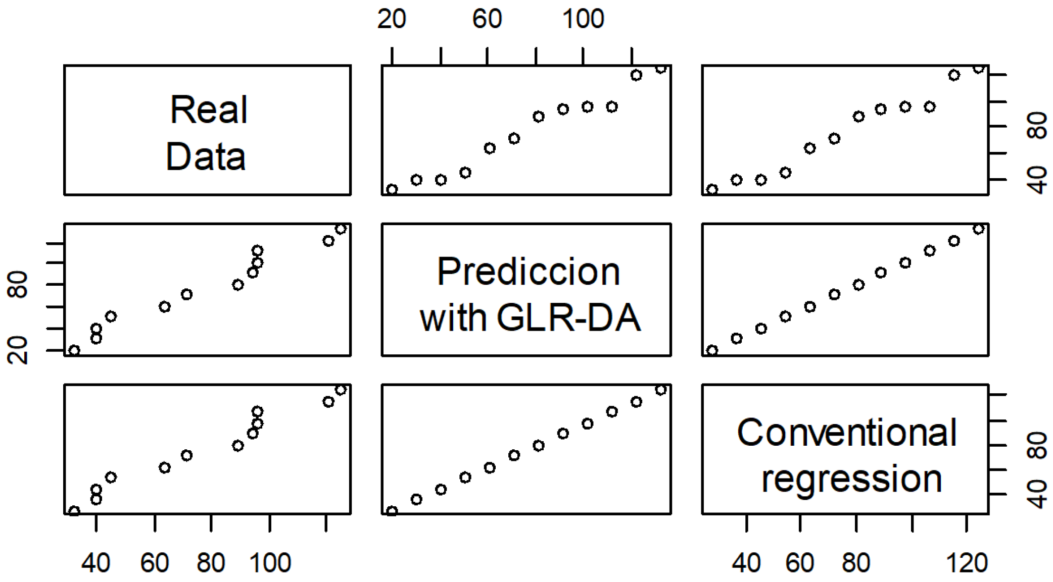
Thus, a cross-validation of the correlation of the information is presented in Figure 3. In fact, the chart presented is very interesting, showing the correlation of the data analyzed with proposed GLR-DA and the conventional linear regression method.

In addition, the box plot is presented in Figure 4. The data analyzed show small variations with respect to their means.

A statistical summary report is depicted in

Table 7. Summary analysis.

Factors	Adj. Total Mean	Adj. Total StDev	Item-Adj Corr.	Cronbach’s Alpha
Real Data	152.16	68.03	0.9828	0.995
Prediction with GLR-DA	152.17	63.49	0.9956	0.9912
Conventional regression	152.16	68.29	0.9962	0.9874

. It can be considered that the means and standard deviations are similar.

Then, a confidence interval was carried out to validate the information, and the results are depicted in

Table 8. Confidence Interval test.

Factor	N	Mean	StDev	95% CI
Real Data	12	76.08	32.16	(56.43, 5.74)
Prediction with GLR-DA	12	76.1	36.4	(56.4, 5.7)
Conventional regression	12	76.08	31.61	(56.43, 5.74)

. It can be observed that difference does not exist between the means analyzed.

In addition, it can be seen in Figure 5 the confidence interval with tendency within limit.

Hence, information was grouped using the Tukey’s Method [44]. The test was conducted using a 95% confidence, and the results are presented in

Table 9. Tukey Pairwise Comparisons.

Factor	N	Mean	Grouping
Conventional regression	12	76.08	A
Real Data	12	76.08	A
Prediction with GLR-DA	12	76.1	A

. It can be see that the means are not significantly different.

Tukey simultaneous tests for differences of means. In this mode, using a individual confidence level = 98.04%. According to comparison of treatment means by Tukey’s Multiple the findings confirm the consistency about our proposal as shown in

Table 10. Tukey Simultaneous Tests.

Difference of Levels	Difference of Means	SE of Difference	95% CI	T-Value	Adjusted p-Value
Prediction-Real Data	0	13.7	(−33.5, 33.5)	0	1
Conventional-Real Data	0	13.7	(−33.5, 33.5)	0	1
Conventional-Prediction	0	13.7	(−33.5, 33.5)	0	1

.

Using the information presented in Figure 6. It can be observed that the means have similar performances. In this manner, we can determine that they contain the same results.

6. Discussion and Conclusions

The linear regression using dimensional analysis is an alternative manner to obtain forecasts. In addition, the methodology’s findings proposed can potentially manipulate regression situation. Likewise, we carried out the different validations to confirm the consistency and stability of the results. Hence, the means comparisons using Tukey test explain the significant contribution to confirm the proficient results with our proposal. According to the different statistical tests realized, we can confirm the effectiveness of our proposal. In addition, the findings about the results from our proposal are reproducible. Therefore, based on those results, we confirm that our proposal is capable of dealing with efficiency, instability, and minimal error focused on the inventory forecast condition.

The literature revised indicates that linear regression continues to be an important topic to be investigated for academics. Nowadays, advances in technology and complexity are demanding accuracy forecast. At the same time, the companies face challenges in addressing the information in a sophisticated manner. Future research can be addressed to implement fuzzy applications and implement a software environment. In addition, it can be interesting to perform comparisons in other fields, for example, health, economics, agriculture, etc.

References

- Hothorn, T.; Bretz, F.; Westfall, P. Simultaneous inference in general parametric models. Biom J. J. Math. Methods Biosci. 2008, 50, 346–363. [Google Scholar] [CrossRef] [PubMed] [Green Version]
- Liu, M.; Hu, S.; Ge, Y.; Heuvelink, G.B.; Ren, Z.; Huang, X. Using multiple linear regression and random forests to identify spatial poverty determinants in rural China. Spat. Stat. 2020, 42, 100461. [Google Scholar] [CrossRef]
- Cook, J.R.; Stefanski, L.A. Simulation-extrapolation estimation in parametric measurement error models. J. Am. Stat. Assoc. 1994, 89, 1314–1328. [Google Scholar] [CrossRef]
- Park, J.Y.; Phillips, P.C. Statistical inference in regressions with integrated processes: Part 2. Econom. Theory 1989, 5, 95–131. [Google Scholar] [CrossRef] [Green Version]
- Johnston, F.; Boylan, J.E.; Shale, E.A. An examination of the size of orders from customers, their characterisation and the implications for inventory control of slow moving items. J. Oper. Res. Soc. 2003, 54, 833–837. [Google Scholar] [CrossRef]
- Babai, M.; Chen, H.; Syntetos, A.; Lengu, D. A compound-Poisson Bayesian approach for spare parts inventory forecasting. Int. J. Prod. Econ. 2021, 232, 107954. [Google Scholar] [CrossRef]
- Mansur, A.; Kuncoro, T. Product inventory predictions at small medium enterprise using market basket analysis approach-neural networks. Procedia Econ. Financ. 2012, 4, 312–320. [Google Scholar] [CrossRef] [Green Version]
- Dekker, R.; Bloemhof, J.; Mallidis, I. Operations Research for green logistics–An overview of aspects, issues, contributions and challenges. Eur. J. Oper. Res. 2012, 219, 671–679. [Google Scholar] [CrossRef] [Green Version]
- Bakker, M.; Riezebos, J.; Teunter, R.H. Review of inventory systems with deterioration since 2001. Eur. J. Oper. Res. 2012, 221, 275–284. [Google Scholar] [CrossRef]
- Saha, E.; Ray, P.K. Modelling and analysis of inventory management systems in healthcare: A review and reflections. Comput. Ind. Eng. 2019, 137, 106051. [Google Scholar] [CrossRef]
- van Steenbergen, R.; Mes, M. Forecasting demand profiles of new products. Decis. Support Syst. 2020, 139, 113401. [Google Scholar] [CrossRef]
- Kourentzes, N.; Trapero, J.R.; Barrow, D.K. Optimising forecasting models for inventory planning. Int. J. Prod. Econ. 2020, 225, 107597. [Google Scholar] [CrossRef] [Green Version]
- Wilson, B.T.; Knight, J.F.; McRoberts, R.E. Harmonic regression of Landsat time series for modeling attributes from national forest inventory data. ISPRS J. Photogramm. Remote Sens. 2018, 137, 29–46. [Google Scholar] [CrossRef]
- Seifbarghy, M.; Amiri, M.; Heydari, M. Linear and nonlinear estimation of the cost function of a two-echelon inventory system. Sci. Iran. 2013, 20, 801–810. [Google Scholar]
- Ryu, S.; Noh, J.; Kim, H. Deep neural network based demand side short term load forecasting. Energies 2017, 10, 3. [Google Scholar] [CrossRef]
- Dalla Corte, A.P.; Souza, D.V.; Rex, F.E.; Sanquetta, C.R.; Mohan, M.; Silva, C.A.; Zambrano, A.M.A.; Prata, G.; de Almeida, D.R.A.; Trautenmüller, J.W.; et al. Forest inventory with high-density UAV-Lidar: Machine learning approaches for predicting individual tree attributes. Comput. Electron. Agric. 2020, 179, 105815. [Google Scholar] [CrossRef]
- Junttila, V.; Laine, M. Bayesian principal component regression model with spatial effects for forest inventory variables under small field sample size. Remote Sens. Environ. 2017, 192, 45–57. [Google Scholar] [CrossRef]
- Ulrich, M.; Jahnke, H.; Langrock, R.; Pesch, R.; Senge, R. Distributional regression for demand forecasting in e-grocery. Eur. J. Oper. Res. 2021, 294, 831–842. [Google Scholar] [CrossRef] [Green Version]
- Georgi, H. Generalized dimensional analysis. Phys. Lett. 1993, 298, 187–189. [Google Scholar] [CrossRef] [Green Version]
- Butterfield, R. Dimensional analysis for geotechnical engineers. Geotechnique 1999, 49, 357–366. [Google Scholar] [CrossRef]
- Cheng, Y.T.; Cheng, C.M. Scaling, dimensional analysis, and indentation measurements. Mater. Sci. Eng. R Rep. 2004, 44, 91–149. [Google Scholar] [CrossRef]
- Bellamine, F.; Elkamel, A. Model order reduction using neural network principal component analysis and generalized dimensional analysis. Eng. Comput. 2008, 25, 443–463. [Google Scholar] [CrossRef]
- Moran, M.; Marshek, K. Some matrix aspects of generalized dimensional analysis. J. Eng. Math. 1972, 6, 291–303. [Google Scholar] [CrossRef]
- Longo, S. Principles and Applications of Dimensional Analysis and Similarity; Springer Nature Switzerland AG: Cham, Switzerland, 2022. [Google Scholar]
- Szava, I.R.; Sova, D.; Peter, D.; Elesztos, P.; Szava, I.; Vlase, S. Experimental Validation of Model Heat Transfer in Rectangular Hole Beams Using Modern Dimensional Analysis. Mathematics 2022, 10, 409. [Google Scholar] [CrossRef]
- Szirtes, T. Applied Dimensional Analysis and Modeling; Butterworth-Heinemann: Oxford, UK, 2007. [Google Scholar]
- Shen, W.; Lin, D.K. Statistical theories for dimensional analysis. Stat. Sin. 2019, 29, 527–550. [Google Scholar] [CrossRef]
- Shen, W.; Davis, T.; Lin, D.K.; Nachtsheim, C.J. Dimensional analysis and its applications in statistics. J. Qual. Technol. 2014, 46, 185–198. [Google Scholar] [CrossRef]
- Albrecht, M.C.; Nachtsheim, C.J.; Albrecht, T.A.; Cook, R.D. Experimental design for engineering dimensional analysis. Technometrics 2013, 55, 257–270. [Google Scholar] [CrossRef]
- Bridgman, P.W. Dimensional Analysis; Yale University Press: New Haven, CT, USA, 1922. [Google Scholar]
- Gibbings, J.C. Dimensional Analysis; Springer Nature & Business Media: New York, NY, USA, 2011. [Google Scholar]
- Dovi, V.; Reverberi, A.; Maga, L.; De Marchi, G. Improving the statistical accuracy of dimensional analysis correlations for precise coefficient estimation and optimal design of experiments. Int. Commun. Heat Mass Transf. 1991, 18, 581–590. [Google Scholar] [CrossRef]
- Breiman, L. Bagging predictors. Mach. Learn. 1996, 24, 123–140. [Google Scholar] [CrossRef] [Green Version]
- Kohli, S.; Godwin, G.T.; Urolagin, S. Sales Prediction Using Linear and KNN Regression. In Advances in Machine Learning and Computational Intelligence; Springer: Singapore, 2021; pp. 321–329. [Google Scholar]
- Gentleman, J.F. New developments in statistical computing. Am. Stat. 1986, 40, 228–237. [Google Scholar] [CrossRef]
- Liang, K.Y.; Zeger, S.L. Longitudinal data analysis using generalized linear models. Biometrika 1986, 73, 13–22. [Google Scholar] [CrossRef]
- Prion, S.K.; Haerling, K.A. Making Sense of Methods and Measurements: Simple Linear Regression. Clin. Simul. Nurs. 2020, 48, 94–95. [Google Scholar] [CrossRef]
- Kuhn, M.; Johnson, K. Applied Predictive Modeling; Springer: New York, NY, USA, 2013; Volume 26. [Google Scholar]
- Wright, J.; Yang, A.Y.; Ganesh, A.; Sastry, S.S.; Ma, Y. Robust face recognition via sparse representation. IEEE Trans. Pattern Anal. Mach. Intell. 2008, 31, 210–227. [Google Scholar] [CrossRef] [PubMed] [Green Version]
- Cheng, J.; Ai, M. Optimal designs for panel data linear regressions. Stat. Probab. Lett. 2020, 163, 108769. [Google Scholar] [CrossRef]
- Huseyin Tunc, B.G. A column generation based heuristic algorithm for piecewise linear regression. Expert Syst. Appl. 2021, 171, 114539. [Google Scholar] [CrossRef]
- Fieller, E.C.; Hartley, H.O.; Pearson, E.S. Tests for rank correlation coefficients. I. Biometrika 1957, 44, 470–481. [Google Scholar] [CrossRef]
- Conrad, S. Sales data and the estimation of demand. J. Oper. Res. Soc. 1976, 27, 123–127. [Google Scholar] [CrossRef]
- Tukey, J.W. Comparing individual means in the analysis of variance. Biometrics 1949, 5, 99–114. [Google Scholar] [CrossRef]
Figure 1.
Normal Distribution.
Figure 2.
Normal Test.
Figure 3.
Correlation Chart about the comparisons.
Figure 4.
Box Plot Chart.
Figure 5.
Confidence interval.
Figure 6.
Tukey simultaneous 95% confidence intervals.