Novel Methods for the Global Synchronization of the Complex Dynamical Networks with Fractional-Order Chaotic Nodes

Abstract

The global synchronization of complex networks with fractional-order chaotic nodes is investigated via a simple Lyapunov function and the feedback controller in this paper. Firstly, the GMMP method is proposed to obtain the numerical solution of the fractional-order nonlinear equation based on the relation of the fractional derivatives. Then, the new feedback controllers are proposed to achieve synchronization between the complex networks with the fractional-order chaotic nodes based on feedback control. We propose some new sufficient synchronous criteria based on the Lyapunov stability and a simple Lyapunov function. By the numerical simulations of the complex networks, we find that these synchronous criteria can apply to the arbitrary complex dynamical networks with arbitrary fractional-order chaotic nodes. Numerical simulations of synchronization between two complex dynamical networks with the fractional-order chaotic nodes are given by the GMMP method and the Newton method, and the results of numerical simulation demonstrate that the proposed method is universal and effective.

1. Introduction

In the last decades, complex dynamical networks have been the subject of worldwide attention because of their wide and important applications in various fields. Many practical complex systems can be modeled by complex dynamical networks, such as gene networks [1], biological networks [2], the World Wide Web [3], ecological complex networks [4], and neural networks [5,6,7]. Synchronization is the one important aspect of the many dynamical behaviors of complex networks. There are a large number of meaningful and important works about the synchronization of networks, such as pinning synchronization [8], projective synchronization [9,10], adaptive synchronization [11,12], and impulsive synchronization [13,14].

Therefore, there are many works about the synchronization of complex networks with various large-scale [15]. In [11], the authors studied a general criterion of networks which can be extended to be much larger sizes than those in other papers. In [16], the authors studied the problem of controllability of a realistic neuronal network of the cat under constraints on control gains. The exponential synchronization issue of general chaotic neural networks was studied in [17]. The synchronization manifold is defined based on a distance from the collective states, and the global synchronization method for the coupled systems was given in [18]. Furthermore, the synchronization of complex networks by the local synchronization of networks was investigated by transferring the stability theory to the synchronization manifold. They also discussed the synchronization of complex network on small-world and scale-free networks in [19,20]. The authors used the means of evolutionary algorithms to study the problem of robust adaptive synchronization between the complex dynamical networks with stochastic coupling [21].

However, many of the above research works mainly studied the synchronization of the complex dynamical networks with integer-order derivatives. The fractional derivative, which is a generalization of the integer derivative, has been the subject of worldwide attention because of its various applications in physics and engineering in recent years [22,23]. The complex dynamical networks with fractional-order nodes have more complex dynamical behaviors than integer-order networks. Then, many studies have shown that complex dynamical networks with fractional-order chaotic nodes have various applications in many fields. Hence, it is essential to study the complex dynamical networks with fractional-order chaotic nodes, especially the synchronization methods for the complex networks. To our knowledge, there is a lot of research on the synchronization method for complex dynamical networks with fractional-order chaotic nodes. The authors presented a fully decentralized adaptive scheme for solving the complex projective synchronization (CPS) in drive-response fractional complex-variable networks, which is a open problem [24]. In [25], the synchronized motions of the N-coupled incommensurate fractional chaotic systems are studied with ring connection. In [26], we have studied the pining control problem about the fractional-order weighted complex dynamical networks. In [27], authors studied the outer synchronization methods for the uncertain networks with adaptive scaling function and different node numbers. The authors studied the synchronization of two networks with fractional-order Liu chaotic oscillators by applying the results of complex systems theory with integer-order systems [28]. In [29], the outer synchronization methods were studied for complex dynamical networks with different fractional-order nodes by adding controller to all nodes. In [30], the authors used an open-plus-closed-loop scheme to study the outer synchronization of two coupled complex networks with fractional-order chaotic nodes. The authors proposed the synchronized motions of a star-shaped complex network with the coupled fractional-order systems [31]. In [32], the authors investigated the synchronization of the complex networks with fractional-order chaotic nodes about a general linear dynamics under directed connected topology. A fractional-order controller was presented for inner and outer synchronization of complex network [33,34] with fractional-order chaotic nodes. In [35], the authors studied the synchronization and anti-synchronization methods for the integer-order complex networks and fractional-order chaotic systems. Moreover, a synchronization method for fractional-order complex dynamical networks was proposed by the fractional-order Proportional Integral (PI) pinning control scheme [36]. The authors used a modified Lyapunov–Krasovakii function to study the exponential sampling synchronization of complex network systems based on the TCS fuzzy model [37]. A general theorem was established for analyzing both the local and global bounded synchronization of a class of heterogeneous networks in a unified approach [38]. The authors proposed the linear feedback synchronization and anti-synchronization methods for a kind of fractional-order chaotic systems based on the triangular structure [39]. The active control method for the synchronization of two different pairs of fractional-order systems were studied [40]. By the linear and adaptive feedback control strategies, the cluster synchronization method was studied for fractional-order complex dynamical networks in [41]. The authors used the pinning control to study the problem of the synchronization of singular complex networks with time-varying delay using Lyapunov–Krasovskii functions and effective mathematical techniques [42].

Hence, in our paper, we study some properties of the fractional derivative, and the numerical method of fractional-order nonlinear equations firstly. Then, a linear feedback controller for the synchronization of the complex dynamical network with fractional-order chaotic nodes is presented. In the following, some sufficient synchronous methods are presented based on the Lyapunov stability theory and a simple Lyapunov function. These methods could apply to the arbitrary complex networks with fractional-order chaotic nodes. Hence, this synchronous method is more general and effective than other methods. For obtaining the numerical solution the fractional-order nonlinear equation, the GMMP method and the Newton method is proposed by the relation of the fractional derivative. All numerical simulations of the two complex dynamical networks with different fractional-order chaotic nodes demonstrate the universality and the effectiveness of the proposed method.

The rest of the paper is described as follows: The preliminaries, definitions, and properties of the fractional derivative and numerical methods of fractional equations are presented in Section 2. Some synchronous control methods of fractional-order complex dynamical networks are given in Section 3. In Section 4, the results of numerical simulation for the fractional-order complex dynamical networks show the universality and effectiveness of the proposed method. The conclusions are given in Section 5 finally.

2. Fractional-Order Equation and Model Description

2.1. Fractional-Order Derivative and Numerical Method of Differential Equation

The fractional derivative, which is a generalization of the integer derivative, has been the subject of worldwide attention because of its various application in physics and engineering [25]. Many definitions of fractional derivatives are studied in many different fields. We will study the three most frequently used definitions of fractional derivatives: the Grunwald–Letnikov (GL) definition, the Riemann–Liouville (RL) definition and the Caputo definition [26], which are equivalent under some conditions. There are some other definitions, such as Abel, Weyl, Fourier, Nishimoto, Cauchy, etc. The Caputo definition is mainly adopted in this paper since it has more advantages embracing well-understood features of physical situation and extensive applicability in depicting real-world problems.

Then, some definitions and properties are given in the following [14].

Definition 1.

The fractional integral of the function $g\left(t\right)$ with order β can be expressed as follows:

$$\begin{array}{c}\hfill {}_a{\mathbf{I}}_t^{\beta }g\left(t\right)={}_a{\mathbf{D}}_t^{-\beta }g\left(t\right)=\frac{1}{\Gamma \left(\beta \right)}{\int }_a^t{(t-\tau )}^{\beta -1}g\left(\tau \right)d\tau \end{array}$$

(1)

for $\beta >0$, $a\in \mathbb{R}$, where $\Gamma \left(z\right)={\int }_0^{\infty }{t}^{z-1}{e}^{-t}dt$ is the Euler’s Gamma function.

Definition 2.

The Riemann–Liouville definition of fractional derivative with the order β for the function $g\left(t\right)$ is defined by:

$$\begin{array}{c}\hfill {}_a^{RL}{\mathbf{D}}_t^{\beta }g\left(t\right)=\frac{d^n}{d{t}^n}{}_a{\mathbf{D}}_t^{-(n-\beta )}g\left(t\right)=\frac{1}{\Gamma (n-\beta )}\frac{d^n}{d{t}^n}{\int }_a^t{(t-\tau )}^{n-\beta -1}g\left(\tau \right)d\tau ,\end{array}$$

(2)

where $n-1<\beta <n,n\in Z^{+}$.

Definition 3.

The Grünwald–Letnikov definition of a fractional derivative with the order β for the function $g\left(t\right)$ is defined by:

$$\begin{array}{cc}\hfill {}_a^{GL}{D}_t^{\beta }g\left(t\right)& =\underset{\begin{array}{c}h\to 0\\ mh=t\end{array}}{lim}{h}^{-\beta }\sum _{r=0}^m{(-1)}^r\left(\genfrac{}{}{0pt}{}{\beta }{r}\right)g(t-rh)\hfill \\ & =\sum _{k=0}^{n-1}\frac{g^{\left(k\right)}\left(0\right)t^{k-\beta }}{\Gamma (k+1-\beta )}+\frac{1}{\Gamma (n-\beta )}·{\int }_a^t{(t-\tau )}^{n-\beta -1}{g}^{\left(n\right)}\left(\tau \right)d\tau ,\hfill \end{array}$$

(3)

where $n-1<\beta <n$.

Definition 4.

The Caputo definition of the fractional derivative with the order β for the function $g\left(t\right)$ can be written as:

$$\begin{array}{c}\hfill {}_a^C{\mathbf{D}}_t^{\beta }g\left(t\right)={}_0{\mathbf{D}}_t^{-(n-\beta )}\frac{d^n}{d{t}^n}g\left(t\right)=\frac{1}{\Gamma (n-\beta )}{\int }_a^t{(t-\tau )}^{n-\beta -1}{g}^{\left(n\right)}\left(\tau \right)d\tau ,\end{array}$$

(4)

where $n-1<\beta <n,n\in Z^{+}$.

Since the difference of the definitions for fractional-order derivatives, the Grünwald–Letnikov fractional derivatives is equivalent to the Riemann–Liouville derivatives. However, the Riemann–Liouville is not equivalent to the Caputo definition. Their relation can be given as:

$${}_a^C{\mathbf{D}}_t^{\beta }g\left(t\right)={}_a^{RL}{\mathbf{D}}_t^{\beta }g\left(t\right)-\sum _{i=0}^{n-1}\frac{{(t-a)}^{i-\beta }{g}^{\left(i\right)}\left(a\right)}{\Gamma (i-\beta +1)}.$$

(5)

According to the relation (5), we find that the Riemann–Liouville and Caputo definitions are also equivalent when the function $g\left(t\right)$ satisfies all initial values $g^{\left(i\right)}\left(a\right)=0,i=0,1,\cdots ,n-1$. Hence, we will prove another relation in the following lemma.

Lemma 1.

Suppose the function $g\left(t\right)\in {\mathbb{C}}^n[a,T]$, then:

$${}_a^C{\mathbf{D}}_t^{\beta }g\left(t\right)={}_a^{RL}{\mathbf{D}}_t^{\beta }(g\left(t\right)-\sum _{k=0}^{n-1}\frac{{(t-a)}^k{g}^k\left(a\right)}{k!}).$$

(6)

where $n-1<\beta \le n.$

Proof. 

We can use the relation (5) and the definition of the Caputo derivative to prove the relation (6). Firstly, let us suppose that:

$$h\left(t\right)=g\left(t\right)-\sum _{k=0}^{n-1}\frac{{(t-a)}^k{g}^{\left(k\right)}\left(a\right)}{k!}.$$

(7)

We can easily obtain that $h^{\left(k\right)}\left(a\right)=0,k=0,1,\cdots ,n-1$. By applying the relation (5), we can obtain ${}_a^C{\mathbf{D}}_t^{\beta }h\left(t\right)={}_a^{RL}{\mathbf{D}}_t^{\beta }h\left(t\right)$, i.e.,:

$${}_a^C{\mathbf{D}}_t^{\beta }h\left(t\right)={}_a^{RL}{\mathbf{D}}_t^{\beta }h\left(t\right)={}_a^{RL}{\mathbf{D}}_t^{\beta }(g\left(t\right)-\sum _{k=0}^{n-1}\frac{{(t-a)}^k{g}^{\left(k\right)}\left(a\right)}{k!}).$$

(8)

Then, the conclusion ${}_a^C{\mathbf{D}}_t^{\beta }{(t-a)}^k=0$ with $0\le k<\beta$ can be obtained by the definition of the Caputo derivative. It follows from the left side of the Equation (7) that

$${}_a^C{\mathbf{D}}_t^{\beta }h\left(t\right)={}_a^C{\mathbf{D}}_t^{\beta }g\left(t\right).$$

(9)

Hence, the conclusion (6) is obtained. □

In the following, the method of a numerical solution for fractional differential equation is proposed. A discretization of interval $[a,T]$ is given as $a=t_0<t_1<\cdots <t_N=T$ with $t_{i+1}-t_i=h$. By the following formula, the Grünwald–Letnikov and Riemann–Liouville fractional-order derivative can be approximated as follows:

$${}_a^{RL}{\mathbf{D}}_t^{\beta }g\left(t\right)={}_a^{GL}{\mathbf{D}}_t^{\beta }g\left(t\right)=\underset{h\to 0}{lim}\frac{1}{h^{\beta }}\sum _{k=0}^N{c}_k^{\beta }g\left(t_{N-k}\right)\approx \frac{1}{h^{\beta }}\sum _{k=0}^N{c}_k^{\beta }g\left(t_{N-k}\right),$$

(10)

and the Caputo fractional derivative can be approximated as follows:

$${}_a^C{\mathbf{D}}_t^{\beta }g\left(t\right)\approx \frac{1}{h^{\beta }}\sum _{k=0}^N{c}_k^{\beta }(g\left(t_{N-k}\right)-\sum _{j=0}^{n-1}\frac{{(t-a)}^j{g}^{\left(j\right)}\left(a\right)}{j!})$$

(11)

where $c_k^{\beta }={(-1)}^k\left(\genfrac{}{}{0pt}{}{\beta }{k}\right)$ are binomial coefficients.

This scheme is first introduced in [29,30], where it is called the GMMP scheme. Based on this scheme (10), a numerical solution method is given for the fractional-order differential equation. To explain this method, the following fractional-order differential equation is considered:

$$\begin{array}{c}\hfill {}_a{\mathbf{D}}_t^{\beta }x\left(t\right)=g(t,x\left(t\right)),\end{array}$$

(12)

where $0\le t\le T$, the initial conditions are $x^{\left(i\right)}\left(a\right)=x_0^{\left(i\right)}$, $i=0,1,\cdots ,n-1,$ and ${}_a{\mathbf{D}}_t^{\beta }$ is the Riemann–Liouville (or Caputo) fractional derivative.

When ${}_a{\mathbf{D}}_t^{\beta }$ denotes the fractional derivative of the Riemann–Liouville definition using the above Formula (10), we obtain:

$$\sum _{j=0}^N{c}_j^{\beta }x\left(t_{N-j}\right)=h^{\beta }g(t_N,x\left(t_N\right)),$$

(13)

i.e.,

$$x\left(t_N\right)=h^{\beta }g(t_N,x\left(t_N\right))-\sum _{j=1}^N{c}_j^{\beta }x\left(t_{N-j}\right).$$

(14)

When ${}_a{\mathbf{D}}_t^{\beta }$ is the fractional derivative of the Caputo definition using the above Formula (11), we obtain:

$$\sum _{j=0}^N{c}_j^{\beta }(x\left(t_{N-k}\right)-\sum _{i=0}^{n-1}\frac{{(t-a)}^i{x}^{\left(i\right)}\left(a\right)}{i!})=h^{\beta }g(t_N,x\left(t_N\right)),$$

(15)

i.e.,

$$x\left(t_N\right)=h^{\beta }g(t_N,x\left(t_N\right))+\sum _{j=0}^{n-1}\frac{{(t-a)}^j{x}^{\left(j\right)}\left(a\right)}{j!}-\sum _{j=1}^N{c}_j^{\beta }(x\left(t_{N-j}\right)-\sum _{i=0}^{n-1}\frac{{(t-a)}^i{x}^{\left(i\right)}\left(a\right)}{i!}).$$

(16)

Especially, when the fractional-order is $0<\beta \le 1$, the above Formula (16) can be simplified to the following:

$$x\left(t_N\right)=h^{\beta }g(t_N,x\left(t_N\right))+x\left(a\right)-\sum _{j=1}^N{c}_j^{\beta }(x\left(t_{N-j}\right)-x\left(a\right)).$$

(17)

An implicit difference scheme (17) is given by the the Grünwald–Letnikov formula, where the unknown variable $x\left(t_N\right)$ is on both sides of the nonlinear equation. Then, we use the Newton–Raphson method to obtain the value of $x\left(t_N\right)$ from the Equation (17).

The Newton–Raphson method is widely used to solve the above Equation (17), which is a nonlinear equation with $x\left(t_N\right)$. This method is a quick and effective method for obtaining the solution of a nonlinear equation. If a nonlinear equation is $G\left(x\right)=0$, the Newton–Raphson method is given as:

$$x_{n+1}=x_n-J_G{\left(x_n\right)}^{-1}G\left(x_n\right),n=0,1,2,\cdots ,$$

(18)

where the $J_G\left(x_n\right)$ denotes the Jacobian matrix. In this paper, we use the GMMP scheme and the Newton–Raphson method to obtain the numerical solution of the fractional-order equations.

2.2. Some Properties of the Fractional Derivative

There are some useful properties of the fractional derivative with the fractional-order $0<\beta <1$ given in the following property [13,14].

Property 1

(Linearity [13]). The fractional derivative of the Caputo definition is a linear operation, i.e.,:

$${}_a{D}_t^{\beta }(\lambda f\left(t\right)+\mu g\left(t\right))=\lambda {}_a{D}_t^{\beta }f\left(t\right)+\mu {}_a{D}_t^{\beta }g\left(t\right),$$

(19)

where λ and μ are real constants.

In the following, we will give two new properties of fractional derivatives to help us construct a simple Lyapunov function, which is used to achieve synchronization of complex network with fractional-order nodes.

Property 2.

If functions $\mathit{x}\left(t\right)={(x_1\left(t\right),\cdots ,x_n\left(t\right))}^T\in {\mathbb{R}}^n$ have a continuous derivatives in interval $[a,t]$, for any matrix $\mathit{A}$ which is a positive definite, we can obtain:

$${}_a^C{D}_t^{\beta }\left(\frac{1}{2}{\mathit{x}}^T\left(t\right)\mathit{A}\mathit{x}\left(t\right)\right)\le {\mathit{x}}^T\left(t\right)\mathit{A}{}_a^C{D}_t^{\beta }\mathit{x}\left(t\right),\forall \beta \in (0,1),$$

(20)

where ${}_a^C{D}_t^{\beta }$ is the fractional derivative of the Caputo definition.

Proof. 

Firstly, let

$$g\left(t\right)={}_a^C{D}_t^{\beta }\left(\frac{1}{2}{\mathit{x}}^T\left(t\right)\mathit{A}\mathit{x}\left(t\right)\right)-{\mathit{x}}^T\left(t\right)\mathit{A}{}_a^C{D}_t^{\beta }\mathit{x}\left(t\right).$$

(21)

Then, we find that Formula (20) is equivalent to the following expression:

$$g\left(t\right)=\frac{1}{2}{}_a^C{D}_t^{\beta }\left({\mathit{x}}^T\left(t\right)\mathit{A}\mathit{x}\left(t\right)\right)-{\mathit{x}}^T\left(t\right)\mathit{A}{}_a^C{D}_t^{\beta }\mathit{x}\left(t\right)\le 0.$$

(22)

It follows from the Caputo definition (4) that the function $g\left(t\right)$ (22) can be rewritten as:

$$\begin{array}{cc}\hfill g\left(t\right)& =\frac{1}{\Gamma (1-\beta )}{\int }_a^t\frac{{\mathit{x}}^T\left(\tau \right)\mathit{A}\dot{\mathit{x}}\left(\tau \right)}{{(t-\tau )}^{\beta }}d\tau -\frac{1}{\Gamma (1-\beta )}{\mathit{x}}^T\left(t\right)\mathit{A}{\int }_a^t\frac{\dot{\mathit{x}}\left(\tau \right)}{{(t-\tau )}^{\beta }}d\tau \hfill \\ & =\frac{1}{\Gamma (1-\beta )}{\int }_a^t\frac{{\mathit{x}}^T\left(\tau \right)\mathit{A}\dot{\mathit{x}}\left(\tau \right)-{\mathit{x}}^T\left(t\right)\mathit{A}\dot{\mathit{x}}\left(\tau \right)}{{(t-\tau )}^{\beta }}d\tau \hfill \\ & =\frac{1}{\Gamma (1-\beta )}{\int }_a^t\frac{({\mathit{x}}^T\left(\tau \right)-{\mathit{x}}^T\left(t\right))\mathit{A}\dot{\mathit{x}}\left(\tau \right)}{{(t-\tau )}^{\beta }}d\tau \hfill \\ & \stackrel{\mathit{z}\left(\tau \right)=\mathit{x}\left(\tau \right)-\mathit{x}\left(t\right)}{=}\frac{1}{\Gamma (1-\beta )}{\int }_a^t\frac{{\mathit{z}}^T\left(\tau \right)\mathit{A}\dot{\mathit{z}}\left(\tau \right)}{{(t-\tau )}^{\beta }}d\tau \hfill \\ & \stackrel{{\mathit{z}}^T\left(\tau \right)\mathit{A}\dot{\mathit{z}}\left(\tau \right)d\tau =\frac{1}{2}d\left({\mathit{z}}^T\left(\tau \right)A\mathit{z}\left(\tau \right)\right)}{=}\frac{1}{2\Gamma (1-\beta )}{\int }_a^t{(t-\tau )}^{-\beta }d\left({\mathit{z}}^T\left(\tau \right)\mathit{A}\mathit{z}\left(\tau \right)\right).\hfill \end{array}$$

(23)

Integrating Formula (23) by parts, we can obtain the function $g\left(t\right)$ as:

$$\begin{array}{cc}\hfill g\left(t\right)& =\frac{1}{2\Gamma (1-\beta )}\frac{{\mathit{z}}^T\left(\tau \right)\mathit{A}\mathit{z}\left(\tau \right)}{{(t-\tau )}^{\beta }}{|}_a^t-\frac{\beta }{2\Gamma (1-\beta )}{\int }_a^t\frac{{\mathit{z}}^T\left(\tau \right)\mathit{A}\mathit{z}\left(\tau \right)}{{(t-\tau )}^{\beta +1}}d\tau \hfill \\ & =\frac{{\mathit{z}}^T\left(\tau \right)\mathit{A}\mathit{z}\left(\tau \right)}{2\Gamma (1-\beta ){(t-\tau )}^{\beta }}{|}_{\tau =t}-\frac{{\mathit{z}}^T\left(a\right)\mathit{A}\mathit{z}\left(a\right)}{2\Gamma (1-\beta ){(t-a)}^{\beta }}-\frac{\beta }{2\Gamma (1-\beta )}{\int }_a^t\frac{{\mathit{z}}^T\left(\tau \right)\mathit{A}\mathit{z}\left(\tau \right)}{{(t-\tau )}^{\beta +1}}d\tau .\hfill \end{array}$$

(24)

Checking the first term of the Formula (24), which has an indetermination at $\tau =t$, we can use the L’Hopital rule to analyze the corresponding limitation:

$$\underset{\tau \to t}{lim}\frac{{\mathit{z}}^T\left(\tau \right)\mathit{A}\mathit{z}\left(\tau \right)}{{(t-\tau )}^{\beta }}=\underset{\tau \to t}{lim}\frac{2{\mathit{z}}^T\left(\tau \right)\mathit{A}\dot{\mathit{z}}\left(\tau \right)}{-\beta {(t-\tau )}^{\beta -1}}=\underset{\tau \to t}{lim}\frac{2{\mathit{z}}^T\left(\tau \right)\mathit{A}\dot{\mathit{z}}\left(\tau \right){(t-\tau )}^{1-\beta }}{-\beta }=0.$$

(25)

It follows from the positive definite matrix $\mathit{A}$ that:

$$\frac{{\mathit{z}}^T\left(a\right)\mathit{A}\mathit{z}\left(a\right)}{2\Gamma (1-\beta ){(t-a)}^{\beta }}\ge 0,$$

(26)

and

$$\frac{\beta }{2\Gamma (1-\beta )}{\int }_a^t\frac{{\mathit{z}}^T\left(\tau \right)\mathit{A}\mathit{z}\left(\tau \right)}{{(t-\tau )}^{\beta +1}}d\tau \ge 0.$$

(27)

Finally, $g\left(t\right)\le 0$ is obtained, i.e., we obtain the conclusion (20). □

Property 3.

If functions $\mathit{x}\left(t\right)={(x_1\left(t\right),\cdots ,x_n\left(t\right))}^T\in {\mathbb{R}}^n$ have a continuous derivatives in $[a,t]$, for any positive definite matrix $\mathit{A}$, we have:

$${}_a^R{D}_t^{\beta }(\frac{1}{2}{\mathit{x}}^T\left(t\right)\mathit{A}\mathit{x}\left(t\right))\le {\mathit{x}}^T\left(t\right)\mathit{A}{}_a^R{D}_t^{\beta }\mathit{x}\left(t\right).\forall \beta \in (0,1)$$

(28)

where the ${}_a^R{D}_t^{\beta }$ is the fractional derivative of the Riemann–Liouville definition.

Proof. 

Firstly, suppose:

$$g\left(t\right)={}_a^R{D}_t^{\beta }(\frac{1}{2}{\mathit{x}}^T\left(t\right)\mathit{A}\mathit{x}\left(t\right))-{\mathit{x}}^T\left(t\right)\mathit{A}{}_a^R{D}_t^{\beta }\mathit{x}\left(t\right),$$

(29)

and we find that the expression (28) is equivalent to the following formula:

$$g\left(t\right)=\frac{1}{2}{}_a^R{D}_t^{\beta }\left({\mathit{x}}^T\left(t\right)\mathit{A}\mathit{x}\left(t\right)\right)-{\mathit{x}}^T\left(t\right)\mathit{A}{}_a^R{D}_t^{\beta }\mathit{x}\left(t\right)\le 0.$$

(30)

It follows from the Riemann–Liouville definition (3) that the function (30) can be rewritten as:

$$\begin{array}{cc}\hfill g\left(t\right)& =\frac{1}{2\Gamma (1-\beta )}\frac{d}{dt}{\int }_a^t\frac{{\mathit{x}}^T\left(\tau \right)\mathit{A}\mathit{x}\left(\tau \right)}{{(t-\tau )}^{\beta }}d\tau -\frac{1}{\Gamma (1-\beta )}{\mathit{x}}^T\left(t\right)\mathit{A}\frac{d}{dt}{\int }_a^t\frac{\mathit{x}\left(\tau \right)}{{(t-\tau )}^{\beta }}d\tau \hfill \\ & =\frac{1}{\Gamma (1-\beta )}\{\frac{1}{2}\frac{d}{dt}{\int }_a^t\frac{{\mathit{x}}^T\left(\tau \right)\mathit{A}\mathit{x}\left(\tau \right)}{{(t-\tau )}^{\beta }}d\tau -{\mathit{x}}^T\left(t\right)\frac{d}{dt}{\int }_a^t\frac{\mathit{A}\mathit{x}\left(\tau \right)}{{(t-\tau )}^{\beta }}d\tau \}\hfill \end{array}$$

(31)

Let

$$h\left(t\right)=\frac{1}{2}\frac{d}{dt}{\int }_a^t\frac{{\mathit{x}}^T\left(\tau \right)\mathit{A}\mathit{x}\left(\tau \right)}{{(t-\tau )}^{\beta }}d\tau -{\mathit{x}}^T\left(t\right)\frac{d}{dt}{\int }_a^t\frac{\mathit{A}\mathit{x}\left(\tau \right)}{{(t-\tau )}^{\beta }}d\tau .$$

(32)

Then:

$$\begin{array}{cc}\hfill h\left(t\right)& \stackrel{\xi =t-\tau }{=}\frac{1}{2}\frac{d}{dt}{\int }_0^{t-a}\frac{{\mathit{x}}^T(t-\xi )\mathit{A}\mathit{x}(t-\xi )}{{\xi }^{\beta }}d\xi -{\mathit{x}}^T\left(t\right)\frac{d}{dt}{\int }_0^{t-a}\frac{\mathit{A}\mathit{x}(t-\xi )}{{\xi }^{\beta }}d\xi \hfill \\ & =\frac{1}{2}\frac{{\mathit{x}}^T\left(a\right)\mathit{A}\mathit{x}\left(a\right)}{{(t-a)}^{\beta }}+{\int }_0^{t-a}\frac{{\mathit{x}}^T(t-\xi )\mathit{A}\dot{\mathit{x}}(t-\xi )}{{\xi }^{\beta }}d\xi -{\mathit{x}}^T\left(t\right)\{\frac{\mathit{A}\mathit{x}\left(a\right)}{{(t-a)}^{\beta }}+{\int }_0^{t-a}\frac{\mathit{A}\dot{\mathit{x}}(t-u)}{{\xi }^{\beta }}d\xi \}\hfill \\ & =\frac{1}{2}\frac{{\mathit{x}}^T\left(a\right)\mathit{A}\mathit{x}\left(a\right)}{{(t-a)}^{\beta }}-\frac{{\mathit{x}}^T\left(t\right)\mathit{A}\mathit{x}\left(a\right)}{{(t-a)}^{\beta }}+{\int }_0^{t-a}\frac{({\mathit{x}}^T(t-\xi )-{\mathit{x}}^T\left(t\right))\mathit{A}\dot{\mathit{x}}(t-\xi )}{{\xi }^{\beta }}d\xi \hfill \\ & \stackrel{\tau =t-\xi }{=}\frac{1}{2}\frac{{\mathit{x}}^T\left(a\right)\mathit{A}\mathit{x}\left(a\right)}{{(t-a)}^{\beta }}-\frac{{\mathit{x}}^T\left(t\right)\mathit{A}\mathit{x}\left(a\right)}{{(t-a)}^{\beta }}+{\int }_a^t\frac{({\mathit{x}}^T\left(\tau \right)-{\mathit{x}}^T\left(t\right))\mathit{A}\dot{\mathit{x}}\left(\tau \right)}{{(t-\tau )}^{\beta }}\hfill \\ & \stackrel{\mathit{z}\left(\tau \right)=\mathit{x}\left(\tau \right)-\mathit{x}\left(t\right)}{=}\frac{1}{2}\frac{{\mathit{x}}^T\left(a\right)\mathit{A}\mathit{x}\left(a\right)}{{(t-a)}^{\beta }}-\frac{{\mathit{x}}^T\left(t\right)\mathit{A}\mathit{x}\left(a\right)}{{(t-a)}^{\beta }}+{\int }_a^t{(t-\tau )}^{-\beta }d(\frac{1}{2}{\mathit{z}}^T\left(\tau \right)\mathit{A}\mathit{z}\left(\tau \right)).\hfill \end{array}$$

(33)

Integrating Formula (33) by parts, we can obtain the function $h\left(t\right)$, as follows:

$$\begin{array}{cc}\hfill h\left(t\right)& =\frac{1}{2}\frac{{\mathit{x}}^T\left(a\right)\mathit{A}\mathit{x}\left(a\right)}{{(t-a)}^{\beta }}-\frac{{\mathit{x}}^T\left(t\right)\mathit{A}\mathit{x}\left(a\right)}{{(t-a)}^{\beta }}+\frac{1}{2}\frac{{\mathit{z}}^T\left(\tau \right)\mathit{A}\mathit{z}\left(\tau \right)}{{(t-\tau )}^{\beta }}{|}_a^t-\frac{\beta }{2}{\int }_a^t\frac{{\mathit{z}}^T\left(\tau \right)\mathit{A}\mathit{z}\left(\tau \right)}{{(t-\tau )}^{\beta +1}}d\tau \hfill \\ & =\frac{1}{2}\underset{\tau \to t}{lim}\frac{{\mathit{z}}^T\left(\tau \right)\mathit{A}\mathit{z}\left(\tau \right)}{{(t-\tau )}^{\beta }}-\frac{{\mathit{x}}^T\left(t\right)\mathit{A}\mathit{x}\left(t\right)}{2{(t-a)}^{\beta }}-\frac{\beta }{2}{\int }_a^t\frac{{\mathit{z}}^T\left(\tau \right)\mathit{A}\mathit{z}\left(\tau \right)}{{(t-\tau )}^{\beta +1}}d\tau .\hfill \end{array}$$

(34)

The first term of the Formula (34) has an indetermination at $\tau =t$. We can check it to analyze the corresponding limitation by L’Hopital rule:

$$\underset{\tau \to t}{lim}\frac{{\mathit{z}}^T\left(\tau \right)\mathit{A}\mathit{z}\left(\tau \right)}{{(t-\tau )}^{\beta }}=\underset{\tau \to t}{lim}\frac{2{\mathit{z}}^T\left(\tau \right)\mathit{A}\dot{\mathit{z}}\left(\tau \right)}{-\beta {(t-\tau )}^{\beta -1}}=\underset{\tau \to t}{lim}\frac{2{\mathit{z}}^T\left(\tau \right)\mathit{A}\dot{\mathit{z}}\left(\tau \right){(t-\tau )}^{1-\beta }}{-\beta }=0.$$

(35)

The matrix $\mathit{A}$ is positive definite, thus:

$$\frac{{\mathit{x}}^T\left(a\right)P\mathit{x}\left(a\right)}{2{(t-a)}^{\beta }}\ge 0,$$

(36)

and

$$\frac{\beta }{2}{\int }_a^t\frac{{\mathit{z}}^T\left(\tau \right)P\mathit{z}\left(\tau \right)}{{(t-\tau )}^{\beta +1}}d\tau \ge 0.$$

(37)

Hence, $h\left(t\right)\le 0$ is obtained, i.e., if $g\left(t\right)\le 0$ is true, then we can obtain the conclusion (28). □

Remark 1.

In the application, the positive definite matrix can be chosen an identity matrix, i.e.,$\mathit{A}=\mathit{I}$, and the above properties (2) and (3) can be written as:

$${}_a{D}_t^{\beta }\left(\frac{1}{2}{\mathit{x}}^T\left(t\right)\mathit{x}\left(t\right)\right)\le {\mathit{x}}^T\left(t\right){}_a{D}_t^{\beta }\mathit{x}\left(t\right).\forall \beta \in (0,1)$$

(38)

where ${}_a{D}_t^{\beta }$ denotes the Caputo definition ${}_a^C{D}_t^{\beta }$ (or the Riemann–Liouville definition ${}_a^R{D}_t^{\beta }$).

2.3. Stability of Fractional-Order Nonlinear System

A general fractional complex dynamical network consists of N identical nodes, and each node is a n-dimensional fractional-order nonlinear dynamical system. For studying the synchronization for this kind of complex networks with fractional-order nodes, we must first study the stability of fractional nonlinear system. We consider the fractional nonlinear system as follows:

$${}_0{D}_t^{\beta }\mathit{y}\left(t\right)=\mathit{g}(t,\mathit{y}\left(t\right)),$$

(39)

where $\beta$ is the fractional-order of derivative; ${}_0{D}_t^{\beta }$ denotes the Caputo (or Riemann–Liouville) fractional-order derivative; $\mathit{g}={(g_1,g_2,\cdots ,g_n)}^T$ is a vector function and $g_i$ is the continuous differential nonlinear functions; and $\mathit{y}\left(t\right)={(y_1\left(t\right),y_2\left(t\right),\cdots ,y_n\left(t\right))}^T$ is the state variable of the system. We can obtain the equilibrium points of the above system by solving $\mathit{g}\left({\mathit{y}}^{\ast }\right)=0$. In the following, the fractional extension of the Lyapunov direct method is proposed for the fractional nonlinear system [31].

Theorem 1.

Suppose that the fractional-order nonautonomous system (39) has an equilibrium point $\mathit{y}=0$. If there exists a Lyapunov function $V(t,\mathit{y}(t\left)\right)$ and class-$\mathit{K}$ functions ${\kappa }_i(i=1,2,3)$ satisfying

$${\kappa }_1\left(\right|\left|\mathit{y}\left(t\right)\right|\left|\right)\le V(t,\mathit{y}\left(t\right))\le {\kappa }_2\left(\right|\left|\mathit{y}\left(t\right)\right|\left|\right),$$

(40)

$${}_0{D}_t^{\gamma }V(t,\mathit{x}\left(t\right))\le -{\kappa }_3\left(\right|\left|\mathit{x}\left(t\right)\right|\left|\right)$$

(41)

where $\gamma \in (0,1)$, then the equilibrium point of fractional-order system (39) is asymptotically stable.

By the new property of fractional derivatives and the fractional-order extension of the Lyapunov direct method, a suitable Lyapunov function can be used to propose the stability condition of the fractional-order nonlinear system.

Theorem 2.

For the fractional nonlinear system:

$${}_0{D}_t^{\beta }\mathit{y}\left(t\right)=\mathit{g}\left(\mathit{y}\left(t\right)\right),$$

(42)

where $\beta \in (0,1)$ and ${}_0{D}_t^{\beta }$ is the Riemann–Liouville (or Caputo) derivative. Without loss of generality, let ${\mathit{y}}^{\ast }=0$ be the equilibrium point and $\mathit{y}\left(t\right)\in {\mathbb{R}}^n$. If a positive definite matrix $\mathit{A}$ satisfies

$${\mathit{y}}^T\left(t\right)\mathit{A}\mathit{g}\left(\mathit{y}\left(t\right)\right)\le 0,$$

(43)

we can obtain that the origin of the fractional-order nonlinear system (39) is asymptotically stable.

Proof. 

It follows positive definite matrix $\mathit{A}$ that a Lyapunov function is introduced as:

$$V\left(\mathit{y}\left(t\right)\right)=\frac{1}{2}{\mathit{y}}^T\left(t\right)\mathit{A}\mathit{y}\left(t\right).$$

(44)

By the Property 2, we can obtain:

$${}_0{D}_t^{\beta }V\left(\mathit{y}\left(t\right)\right)\le {\mathit{y}}^T\left(t\right)\mathit{A}{}_0{D}_t^{\beta }\mathit{y}\left(t\right)={\mathit{y}}^T\left(t\right)\mathit{A}\mathit{g}\left(\mathit{y}\left(t\right)\right).$$

(45)

It follows ${\mathit{y}}^T\left(t\right)\mathit{A}\mathit{g}\left(\mathit{y}\left(t\right)\right)\le 0$ that the fractional derivative of the Lyapunov function is a negative definite. Due to the relation between class-K functions and positive definite functions in [32], it follows from Theorem (1) that the origin of the fractional-order nonlinear system (39) is asymptotically stable. □

2.4. Instruction of the Complex Dynamical Network with Fractional Order Nodes

A general fractional complex dynamical network consists of N identical nodes, and each node is an n-dimensional fractional nonlinear chaotic system. It can be described as:

$$\begin{array}{c}\hfill {\mathrm{D}}_t^{\beta }{\mathit{x}}_j\left(t\right)=\mathit{g}\left({\mathit{x}}_j\left(t\right)\right)+C\sum _{k=1}^N{p}_{jk}\mathit{A}{\mathit{x}}_k\left(t\right),j=1,2,\cdots ,N,\end{array}$$

(46)

where $\beta \in (0,1)$ is the fractional-order; ${\mathit{x}}_j\left(t\right)={(x_{j1}\left(t\right),x_{j2}\left(t\right),\cdots ,x_{jn}\left(t\right))}^T\in {\mathbb{R}}^n$ denotes the state vector of the ith node; $\mathit{g}:{\mathbb{R}}^n\to {\mathbb{R}}^n$ is a given smooth nonlinear vector field; the dynamics of the ith node is given by the fractional-order equation ${\mathrm{D}}_t^{\beta }{\mathit{x}}_j\left(t\right)=\mathit{g}\left({\mathit{x}}_j\left(t\right)\right)$; $\mathit{A}\in {\mathbb{R}}^{n\times n}$ is the inner-coupling matrix which describes the interactions between the variables of the node itself; C is the coupling strength; $\mathit{P}={\left(p_{jk}\right)}_{n\times n}$ denotes the coupling configuration diffusive matrix representing the topological structure of the network, in which $p_{jk}>0$ if there is a connection from node j to node k$(j\ne k)$, and $p_{jk}=0$$(j\ne k)$ otherwise. The diagonal elements of $\mathit{P}$ are given by $p_{jj}=-{\sum }_{k=1,j\ne k}^N{p}_{jk}$.

We consider the complex network (46) with N fractional-order nodes as a drive network, the response complex network with N fractional-order nodes is given as follows:

$$\begin{array}{c}\hfill {\mathrm{D}}_t^{\beta }{\mathit{y}}_j\left(t\right)=\mathit{g}\left({\mathit{y}}_j\left(t\right)\right)+C\sum _{k=1}^N{p}_{jk}\mathit{A}{\mathit{y}}_k\left(t\right),j=1,2,\cdots ,N,\end{array}$$

(47)

which have the same topological structure and node dynamics as the drive complex network (46). Our aim is to propose a suitable feedback controller to achieve the synchronization of the complex dynamical network (47) and network (46), i.e.,

$$\begin{array}{c}\hfill \underset{t\to \infty }{lim}\left|\right|{\mathit{y}}_j\left(t\right)-{\mathit{x}}_j\left(t\right)\left|\right|=0,1\le j\le N.\end{array}$$

(48)

Adding feedback control to the complex network (47), the controlled response complex network with fractional-order nodes is as follows:

$$\begin{array}{c}\hfill {\mathrm{D}}_t^{\beta }{\mathit{y}}_j\left(t\right)=\mathit{g}\left({\mathit{y}}_j\left(t\right)\right)+C\sum _{k=1}^N{p}_{jk}\mathit{A}{\mathit{y}}_k\left(t\right)+{\mathbf{\psi }}_j({\mathit{x}}_j,{\mathit{y}}_j),j=1,2,\cdots ,N.\end{array}$$

(49)

where ${\mathbf{\psi }}_j:{\mathbb{R}}^n\to {\mathbb{R}}^n(1\le j\le N)$ are all control functions. In the following the mathematical definition of synchronization for complex network with fractional-order nodes is given.

Definition 5.

Let ${\mathit{x}}_j(t;t_0,{\mathit{X}}_0)$ and ${\mathit{y}}_j(t,{\mathit{Y}}_0)(1\le j\le N)$ be the solutions of the complex networks (46) and (49) with fractional-order nodes, respectively, where ${\mathit{X}}_0=(x_{10},x_{20},\cdots ,x_{N0})\in {\mathbb{R}}^{n\times N}$, and $\mathit{g}:\mathsf{\Omega }\to {\mathbb{R}}^n$ is a continuous function. If there is a nonempty subset $\Gamma \subseteq \mathsf{\Omega }$, with $x_{j0},y_{j0}\in \Gamma (1\le j\le N)$, such that ${\mathit{x}}_j(t;t_0,{\mathit{X}}_0),{\mathit{y}}_j(t;t_0,{\mathit{Y}}_0)\in \mathsf{\Omega }$ for all $t>t_0$, and

$$\begin{array}{c}\hfill \underset{t\to \infty }{lim}\left|\right|{\mathit{y}}_j(t,{\mathit{Y}}_0)-{\mathit{x}}_j(t,{\mathit{X}}_0)\left|\right|=0,1\le j\le N,\end{array}$$

(50)

then the response complex network (49) with fractional-order nodes is said to be asymptotically synchronized to the drive network (46).

The error vector is defined by:

$$\begin{array}{c}\hfill {\mathit{e}}_j\left(t\right)={\mathit{y}}_j\left(t\right)-{\mathit{x}}_j\left(t\right),1\le j\le N.\end{array}$$

(51)

Then, the error fractional dynamical system can be given as follows:

$${\mathrm{D}}_t^{\beta }{\mathit{e}}_j\left(t\right)=\mathit{g}\left({\mathit{y}}_j\left(t\right)\right)-\mathit{g}\left({\mathit{x}}_j\left(t\right)\right)+C\sum _{k=1}^N{p}_{jk}\mathit{A}{\mathit{e}}_k\left(t\right)+{\mathbf{\psi }}_j({\mathit{x}}_j,{\mathit{y}}_j),j=1,2,\cdots ,N.$$

(52)

Then, the stabilization of the fractional error dynamical system (52) is equivalent to the synchronization of the complex dynamical networks (46) and (49) with fractional-order nodes.

3. Method of Synchronization Control for the Complex Network with Fractional-Order Nodes

In the following, we would give the synchronization method of the complex network with fractional-order nodes. Firstly, the fractional-order complex network (46) can be rewritten as follows:

$${\mathrm{D}}_t^{\beta }{\mathit{x}}_j\left(t\right)=\mathit{L}{\mathit{x}}_j\left(t\right)+\mathit{h}\left({\mathit{x}}_j\left(t\right)\right)+C\sum _{k=1}^N{p}_{jk}\mathit{A}{\mathit{x}}_k\left(t\right),j=1,2,\cdots ,N,$$

(53)

where $\mathit{L}{\mathit{x}}_{\mathit{j}}\left(t\right)$ is the linear part of network (46), and $\mathit{h}\left({\mathit{x}}_{\mathit{j}}\left(t\right)\right)$ is the nonlinear part of network (46). We find that this way of writing is so general that almost all complex dynamical networks with fractional-order chaotic nodes can be written as this form (53). We consider the complex network (53) is the drive network, then the response network is given as:

$${\mathrm{D}}_t^{\beta }{\mathit{y}}_j\left(t\right)=\mathit{L}{\mathit{y}}_j\left(t\right)+\mathit{h}\left({\mathit{y}}_j\left(t\right)\right)+C\sum _{k=1}^N{p}_{jk}\mathit{A}{\mathit{y}}_k\left(t\right),j=1,2,\cdots ,N.$$

(54)

In order to achieve the synchronization of above two complex networks (53) and (54), a linear feedback control input is added to the response network (54). As we known, the linear controller has many advantages, such as being very simple, easily realized, and more suitable for engineering applications.

With the linear feedback control input, the controlled response complex network (54) can be rewritten as:

$${\mathit{y}}_j\left(t\right)=\mathit{L}{\mathit{y}}_j\left(t\right)+\mathit{h}\left({\mathit{y}}_j\left(t\right)\right)+C\sum _{k=1}^N{p}_{jk}\mathit{A}{\mathit{y}}_k\left(t\right)-K_j({\mathit{y}}_j\left(t\right)-{\mathit{x}}_j\left(t\right)),j=1,2,\cdots ,N,$$

(55)

where the feedback gain matrices $K_j\in {\mathbb{R}}^{n\times n}(j=1,2,\cdots ,N)$ of the linear feedback control input $K_j({\mathit{y}}_j\left(t\right)-{\mathit{x}}_j\left(t\right))$ need to be determined.

The synchronization error is $\mathit{e}(t)={\mathit{y}}_j\left(t\right)-{\mathit{x}}_j\left(t\right),j=1,2,\cdots ,N$, and the fractional-order error system from (53) and (55) is obtained as follows:

$$\begin{array}{cc}\hfill {}_0{D}_t^{\beta }{\mathit{e}}_j\left(t\right)& =\mathit{L}{\mathit{e}}_j\left(t\right)+(\mathit{h}\left({\mathit{y}}_j\left(t\right)\right)-\mathit{h}\left({\mathit{x}}_j\left(t\right)\right))+C\sum _{k=1}^N{g}_{jk}\mathit{A}{\mathit{e}}_k\left(t\right)-K_j{\mathit{e}}_j\left(t\right)\hfill \\ & =\mathit{L}{\mathit{e}}_j\left(t\right)+B_{{\mathit{x}}_{\mathit{j}},{\mathit{y}}_{\mathit{j}}}{\mathit{e}}_j\left(t\right)+C\sum _{k=1}^N{p}_{jk}\mathit{A}{\mathit{e}}_k\left(t\right)-K_j{\mathit{e}}_j\left(t\right),\hfill \end{array}$$

(56)

where $B_{{\mathit{x}}_{\mathit{j}},{\mathit{y}}_{\mathit{j}}}$ a matrices which are bounded to their elements ${\mathit{x}}_{\mathit{j}}$ and ${\mathit{y}}_{\mathit{j}}$, respectively.

Hence, the conclusion can be obtained that the fractional error system (56) is asymptotically stable at the origin point only if the fractional-order networks (53) and (55) are synchronized. Therefore, our objective is to propose the suitable feedback gain matrices $K_i$ which make the fractional error system (56) asymptotically stable.

Theorem 3.

The controlled fractional error system (56) is asymptotically stable at the origin, i.e., the fractional-order complex networks (53) and (55) are asymptotically synchronized, if the feedback gain matrices $K_j$ makes the corresponding symmetric matrix:

$$S_j=\frac{{(L+B_{{\mathit{x}}_{\mathit{j}},{\mathit{y}}_{\mathit{j}}}-K_j)}^T+(L+B_{{\mathit{x}}_{\mathit{j}},{\mathit{y}}_{\mathit{j}}}-K_j)}{2}$$

(57)

be a negative definite matrix for all ${\mathit{x}}_j\left(t\right)$, ${\mathit{y}}_j\left(t\right)$ and $j=1,2,\cdots ,N$.

Proof. 

For the controlled error system (56), we introduce a Lyapunov function as follows:

$$V=\frac{1}{2}\sum _{j=1}^N{\mathit{e}}_i^T\left(t\right){\mathit{e}}_j\left(t\right).$$

(58)

It follows from Properties (2) that

$$\begin{array}{cc}\hfill {}_0{D}_t^{\beta }V& =\frac{1}{2}{}_0{D}_t^{\beta }\sum _{j=1}^N{\mathit{e}}_j^T\left(t\right){\mathit{e}}_j\left(t\right)\hfill \\ & \le \sum _{j=1}^N{\mathit{e}}_j^T\left(t\right){}_0{D}_t^{\beta }{\mathit{e}}_j\left(t\right)\hfill \\ & =\sum _{j=1}^N{\mathit{e}}_j^T\left(t\right)\left(\mathit{L}{\mathit{e}}_j\left(t\right)+B_{{\mathit{x}}_{\mathit{j}},{\mathit{y}}_{\mathit{j}}}{\mathit{e}}_j\left(t\right)+C\sum _{k=1}^N{p}_{jk}\mathit{A}{\mathit{e}}_k\left(t\right)-K_j{\mathit{e}}_j\left(t\right)\right)\hfill \\ & =\sum _{j=1}^N{\mathit{e}}_j^T\left(t\right)\mathit{L}{\mathit{e}}_j\left(t\right)+\sum _{j=1}^N{\mathit{e}}_j^T\left(t\right)B_{{\mathit{x}}_{\mathit{j}},{\mathit{y}}_{\mathit{j}}}{\mathit{e}}_j\left(t\right)+C\sum _{j=1}^N\sum _{k=1}^N{p}_{jk}{\mathit{e}}_j^T\left(t\right)\mathit{A}{\mathit{e}}_k\left(t\right)\hfill \\ & -\sum _{j=1}^N{\mathit{e}}_j^T\left(t\right)K_j{\mathit{e}}_j\left(t\right)\hfill \\ & =\sum _{j=1}^N{\mathit{e}}_j^T\left(t\right)\mathit{L}{\mathit{e}}_j\left(t\right)+\sum _{j=1}^N{\mathit{e}}_j^T\left(t\right)B_{{\mathit{x}}_{\mathit{j}},{\mathit{y}}_{\mathit{j}}}{\mathit{e}}_j\left(t\right)+C\sum _{j=1}^N\sum _{k\ne j}^N{p}_{jk}{\mathit{e}}_j^T\left(t\right)\mathit{A}{\mathit{e}}_k\left(t\right)\hfill \\ & +C\sum _{j=1}^N{p}_{jj}{\mathit{e}}_j^T\left(t\right)\mathit{A}{\mathit{e}}_j\left(t\right)-\sum _{j=1}^N{\mathit{e}}_j^T\left(t\right)K_j{\mathit{e}}_j\left(t\right)\hfill \\ & \le \sum _{j=1}^N{\mathit{e}}_j^T\left(t\right)\mathit{L}{\mathit{e}}_j\left(t\right)+\sum _{j=1}^N{\mathit{e}}_j^T\left(t\right)B_{{\mathit{x}}_{\mathit{j}},{\mathit{y}}_{\mathit{j}}}{\mathit{e}}_j\left(t\right)+\frac{C}{2}\sum _{j=1}^N\sum _{k\ne j}^N{p}_{jk}({\mathit{e}}_j^T\left(t\right)\mathit{A}{\mathit{e}}_j\left(t\right)+{\mathit{e}}_k^T\left(t\right)\mathit{A}{\mathit{e}}_k\left(t\right))\hfill \\ & =\sum _{j=1}^N{\mathit{e}}_j^T\left(t\right)\mathit{L}{\mathit{e}}_j\left(t\right)+\sum _{j=1}^N{\mathit{e}}_j^T\left(t\right)B_{{\mathit{x}}_{\mathit{j}},{\mathit{y}}_{\mathit{j}}}{\mathit{e}}_j\left(t\right)+\frac{C}{2}\sum _{j=1}^N\sum _{k\ne j}^N{p}_{jk}{\mathit{e}}_j^T\left(t\right)\mathit{A}{\mathit{e}}_j\left(t\right)\hfill \\ & +\frac{C}{2}\sum _{j=1}^N\sum _{k\ne j}^N{p}_{jk}{\mathit{e}}_k^T\left(t\right)\mathit{A}{\mathit{e}}_k\left(t\right)+C\sum _{j=1}^N{p}_{jj}{\mathit{e}}_j^T\left(t\right)\mathit{A}{\mathit{e}}_j\left(t\right)-\sum _{j=1}^N{\mathit{e}}_j^T\left(t\right)K_j{\mathit{e}}_j\left(t\right)\hfill \\ & =\sum _{j=1}^N{\mathit{e}}_j^T\left(t\right)\mathit{L}{\mathit{e}}_j\left(t\right)+\sum _{j=1}^N{\mathit{e}}_j^T\left(t\right)B_{{\mathit{x}}_{\mathit{j}},{\mathit{y}}_{\mathit{j}}}{\mathit{e}}_j\left(t\right)-\frac{C}{2}\sum _{j=1}^N{p}_{jj}{\mathit{e}}_j^T\left(t\right)\mathit{A}{\mathit{e}}_j\left(t\right)\hfill \\ & -\frac{C}{2}\sum _{k=1}^N{p}_{kk}{\mathit{e}}_k^T\left(t\right)\mathit{A}{\mathit{e}}_k\left(t\right)+C\sum _{j=1}^N{p}_{jj}{\mathit{e}}_j^T\left(t\right)\mathit{A}{\mathit{e}}_j\left(t\right)-\sum _{j=1}^N{\mathit{e}}_j^T\left(t\right)K_j{\mathit{e}}_j\left(t\right)\hfill \\ & =\sum _{j=1}^N{\mathit{e}}_j^T\left(t\right)\mathit{L}{\mathit{e}}_j\left(t\right)+\sum _{j=1}^N{\mathit{e}}_j^T\left(t\right)B_{{\mathit{x}}_{\mathit{j}},{\mathit{y}}_{\mathit{j}}}{\mathit{e}}_j\left(t\right)-\sum _{j=1}^N{\mathit{e}}_j^T\left(t\right)K_j{\mathit{e}}_j\left(t\right)\hfill \\ & =\sum _{j=1}^N{\mathit{e}}_j^T\left(t\right)\left(\mathit{L}+B_{{\mathit{x}}_{\mathit{j}},{\mathit{y}}_{\mathit{j}}}+K_j\right){\mathit{e}}_j\left(t\right)\hfill \\ & =\sum _{i=1}^N{\mathit{e}}_j^T\left(t\right)S_j{\mathit{e}}_j\left(t\right),\hfill \end{array}$$

(59)

where

$$S_j=\frac{{(L+B_{{\mathit{x}}_{\mathit{j}},{\mathit{y}}_{\mathit{j}}}-K_j)}^T+(L+B_{{\mathit{x}}_{\mathit{j}},{\mathit{y}}_{\mathit{j}}}-K_j)}{2}$$

(60)

is a n-order symmetric square matrix. If $S_j$ is a negative definite matrix for all ${\mathit{x}}_j\left(t\right)$, ${\mathit{y}}_j\left(t\right)$, and $j=1,2,\cdots ,N$, we have

$${}_0{D}_t^{\beta }V\le \sum _{i=1}^N{\mathit{e}}_j^T\left(t\right)S_i{\mathit{e}}_j\left(t\right)<0.$$

(61)

According to Theorem (2), we can obtain the controller to make the fractional error system asymptotically stable at the origin, i.e., the complex networks (53) and (55) with fractional-order nodes are asymptotically synchronized. □

Here, we mainly study the synchronization of complex dynamical networks with fractional-order nodes, and each node is an n-dimensional fractional-order chaotic system. It is well-known that ${\mathit{x}}_j\left(t\right)$ and ${\mathit{y}}_j\left(t\right)$ are bounded in the fractional chaotic system. Hence, it indicates that we can find a constant matrix $M_j$ for any $B_{{\mathit{x}}_j,{\mathit{y}}_j}$, which satisfies:

$${\mathit{e}}_j^T\left(t\right)B_{{\mathit{x}}_j,{\mathit{y}}_j}{\mathit{e}}_j\left(t\right)\le {\mathit{e}}_j^T\left(t\right)M_i{\mathit{e}}_j\left(t\right),$$

(62)

for all $j=1,2,\cdots ,N$. Then, some corollaries can be obtained, which are simpler than the above Theorem (3).

Corollary 1.

The fractional-order complex dynamical networks (53) and (55) are asymptotically synchronized, i.e., the controlled fractional error system (56) is asymptotically stable at the origin, if the feedback gain matrix $K_j,j=1,2,\cdots ,N$ makes the matrix

$$S_j=\frac{{(L+M_j-K_j)}^T+(L+M_j-K_j)}{2}$$

(63)

a negative definite for all $j=1,2,\cdots ,N$, where $M_j$ is given as (62).

We can easily prove this corollary by the Theorem (3) and inequality (62).

If the constant matrix $M_j=m_{j}I$ and the feedback gain matrix $K_j=k_{j}I$, where I is identity matrix and $j=1,2,\cdots ,N$, the simpler corollaries can be obtained as follows.

Corollary 2.

The fractional-order complex dynamical networks (53) and (55) are asymptotically synchronized, i.e., the controlled fractional error system (56) is asymptotically stable at the origin, if the feedback gain matrix $K_i=k_{j}I$ makes the matrix:

$$S_j=\frac{L^T+L}{2}+(m_j-k_j)I$$

(64)

negative definite for all $j=1,2,\cdots ,N$. Especially, let ${\lambda }_{max}$ be the maximal eigenvalue of the matrix $\frac{L^T+L}{2}$, if $K_j=k_{j}I$ satisfies:

$${\lambda }_{max}+m_j-k_j<0,j=1,2,\cdots ,N,$$

(65)

the controlled fractional error system (56) is asymptotically stable at the origin.

Let the constant matrix be $M_j=mI$ and the feedback gain matrix be $K_j=kI$ for all $j=1,2,\cdots ,N$, where I is the identity matrix. The simplest corollary can be given as follows.

Corollary 3.

The fractional-order complex dynamical networks (53) and (55) are asymptotically synchronized, i.e., the controlled fractional error system (56) is asymptotically stable at the origin, if the feedback gain matrix $K_j=kI$ (for all $j=1,2,\cdots ,N$) makes the following matrix

$$S_j=\frac{L^T+L}{2}+(m-k)I$$

(66)

a negative definite. Especially, let ${\lambda }_{max}$ denote the maximal eigenvalue of the symmetric matrix $\frac{L^T+L}{2}$, if $K_j=kI$ satisfies

$${\lambda }_{max}+m-k<0,$$

(67)

the controlled fractional error system (56) is asymptotically stable at the origin.

Remark 2.

In these Theorems and corollaries, we obtain some sufficient conditions for the synchronization of the complex dynamical networks with fractional-order nodes. For easy application, the feedback gain matrix is only chosen as $K_j=kI$ satisfying $k>{\lambda }_{max}+m$, which can make the complex dynamical networks (53) and (55) with N fractional-order nodes synchronize, i.e., the fractional-order error system (56) asymptotically stable at the origin.

Remark 3.

For the Corollary (3), if the constant matrix and feedback gain matrix are chosen as $M_j=mI$ and $K_j=kI$, respectively, the conclusion is also obtained. Furthermore, let those matrices $M_j$ and $K_j$ be diagonal, i.e., the constant matrix and feedback gain matrix are $M_j=diag(m_1,m_2,m_3)$ and $K_j=diag(k_1,k_2,k_3)$, respectively, for all $j=1,2,\cdots ,N$. It follows from Theorem (3) and Corollary (3) that a suitable $k_j$ can be found to satisfy the condition. However, some $k_j$ and $m_j$ are equal to zero in many cases, which can make the linear controller very simpler.

4. Simulation and Analysis of Fractional Complex Networks

In the following, two complex dynamical networks with fractional-order nodes are used as examples to illustrate how to use the synchronization method proposed in this paper to analyze the projective synchronization for complex networks. For obtaining the numerical solution of the fractional-order nonlinear system, we adopt the GMMP scheme and the Newton–Raphson method, which is proposed in Section 2.1.

4.1. Synchronization of the Complex Networks with Eight Fractional-Order Nodes of a Chaotic Liu System

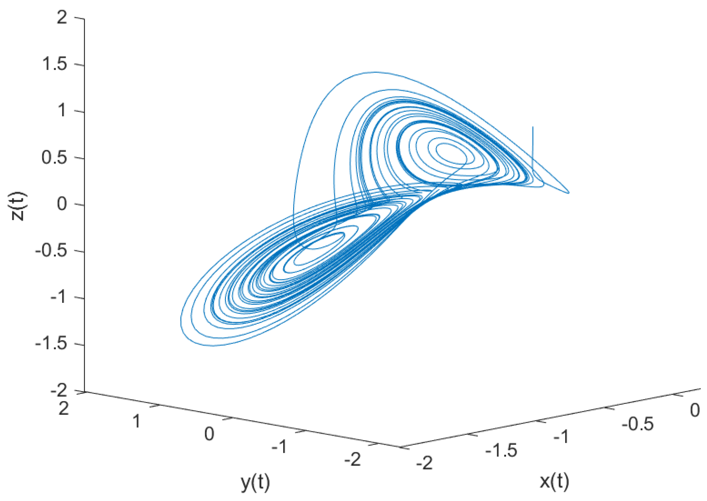
Supposed that the fractional-order dynamical complex networks have eight nodes, and each node can be described by the fractional-order chaotic Liu system [14,33] as follows:

$$\begin{array}{cc}\hfill & {\mathrm{D}}_t^{\beta }{x}_{j1}=a(x_{j2}-x_{j1}),\hfill \\ & {\mathrm{D}}_t^{\beta }{x}_{j2}=b{x}_{j2}-x_{j1}{x}_{j3},\hfill \\ & {\mathrm{D}}_t^{\beta }{x}_{j3}=c{x}_{j1}^2-d{x}_{j3},\hfill \end{array}$$

(68)

where $j=1,2,\cdots ,8$. When we chose the fractional-order $\beta =0.95$ and the parameters as $a=10$, $b=40$, $c=4$, $d=2.5$, the chaotic behavior of the fractional-order chaotic system (68) is shown in Figure 1.

We choose the coupling configuration matrix and the inner matrix of the fractional-order complex network as follows:

$$P={\left(p_{ij}\right)}_{8\times 8}=\left(\begin{array}{cccccccc}-2& 0& 0& 1& 1& 0& 0& 0\\ 0& -2& 1& 0& 0& 1& 0& 0\\ 0& 1& -3& 0& 0& 1& 0& 1\\ 1& 0& 0& -3& 1& 0& 0& 1\\ 1& 0& 0& 1& -3& 0& 1& 0\\ 0& 1& 1& 0& 0& -2& 0& 0\\ 0& 0& 0& 0& 1& 0& -2& 1\\ 0& 0& 1& 1& 0& 0& 1& -3\end{array}\right),A=\left(\begin{array}{ccc}1& 0& 0\\ 0& 1& 0\\ 0& 0& 1\end{array}\right).$$

The drive complex network is given as follows with eight nodes of the fractional-order Liu chaotic system:

$$\begin{array}{c}\hfill {\mathrm{D}}_t^{\beta }{\mathit{x}}_j\left(t\right)=\mathit{f}\left({\mathit{x}}_j\left(t\right)\right)+\sum _{k=1}^N{p}_{jk}\mathit{A}{\mathit{x}}_k\left(t\right),j=1,2,\cdots ,8,\end{array}$$

(69)

which can be rewritten in the form (53):

$$\begin{array}{c}\hfill {\mathrm{D}}_t^{\beta }{\mathit{x}}_j\left(t\right)=\mathit{L}{\mathit{x}}_j\left(t\right)+\mathit{h}\left({\mathit{x}}_j\left(t\right)\right)+\sum _{k=1}^N{p}_{jk}\mathit{A}{\mathit{x}}_k\left(t\right),j=1,2,\cdots ,8,\end{array}$$

(70)

where

$$\mathit{L}=\left(\begin{array}{ccc}-a& a& 0\\ 0& b& 0\\ 0& 0& -d\end{array}\right),$$

(71)

and

$$\mathit{h}\left({\mathit{x}}_j\left(t\right)\right)={(0,-x_{j1}{x}_{j3},c{x}_{j1}^2)}^T.$$

(72)

Adding the controller to the response complex network, the controlled complex network can be written as:

$${\mathrm{D}}_t^q{\mathit{y}}_j\left(t\right)=\mathit{L}{\mathit{y}}_j\left(t\right)+\mathit{h}\left({\mathit{y}}_j\left(t\right)\right)+\sum _{k=1}^N{p}_{jk}\mathit{A}{\mathit{y}}_k\left(t\right)-K_j({\mathit{y}}_j\left(t\right)-{\mathit{x}}_j\left(t\right)),j=1,2,\cdots ,8.$$

(73)

According to complex networks (70) and (73), the controlled error system is obtained:

$$\begin{array}{c}\hfill {\mathrm{D}}_t^q{\mathit{e}}_j\left(t\right)=\mathit{L}{\mathit{e}}_j\left(t\right)+{\mathit{B}}_{x_j,y_j}{\mathit{e}}_j\left(t\right)+\sum _{k=1}^N{p}_{jk}\mathit{A}{\mathit{e}}_k\left(t\right)-K_j{\mathit{e}}_j\left(t\right),j=1,2,\cdots ,8,\end{array}$$

(74)

where ${\mathit{B}}_{x_j,y_j}(j=1,2,\cdots ,N)$ are bounded matrices with their elements depending on ${\mathit{x}}_j$ and ${\mathit{y}}_j$.

Since the fractional-order Liu system is chaotic, ${\mathit{x}}_j\left(t\right)(j=1,2,\cdots ,8)$ and ${\mathit{y}}_j\left(t\right)(j=1,2,\cdots ,8)$ are bounded. It can easily be obtained that ${\mathit{e}}_j^T\left(t\right){\mathit{B}}_{{\mathit{x}}_j,{\mathit{y}}_j}{\mathit{e}}_j\left(t\right)=-x_{j3}{e}_{j1}{e}_{j2}-y_{j1}{e}_{j2}{e}_{j3}+c(x_{j1}+y_{j1})e_{j1}{e}_{j3}\le 10{\mathit{e}}_j^T\left(t\right){\mathit{e}}_j\left(t\right)$ by calculating the eigenvalue of maximum, which implies $m\approx 10$. According to Corollary 2, if the matrices $S_j=\frac{L^T+L}{2}+(m-k)I$ ($j=1,2,\cdots ,8$) are negative positive, the fractional error system (74) is asymptotically stable, i.e., the complex networks (70) and (73) can achieve synchronization. Furthermore, we can easily obtain that the maximal eigenvalue of matrix $\frac{L^T+L}{2}$ is ${\lambda }_{max}\approx 40$. Hence, if the control parameters ${\mathit{k}}_j(j=1,2,\cdots ,8)$ satisfy the conditions of Theorem 1, the complex dynamical networks (70) and (73) can achieve synchronization with eight fractional-order nodes by the linear controllers.

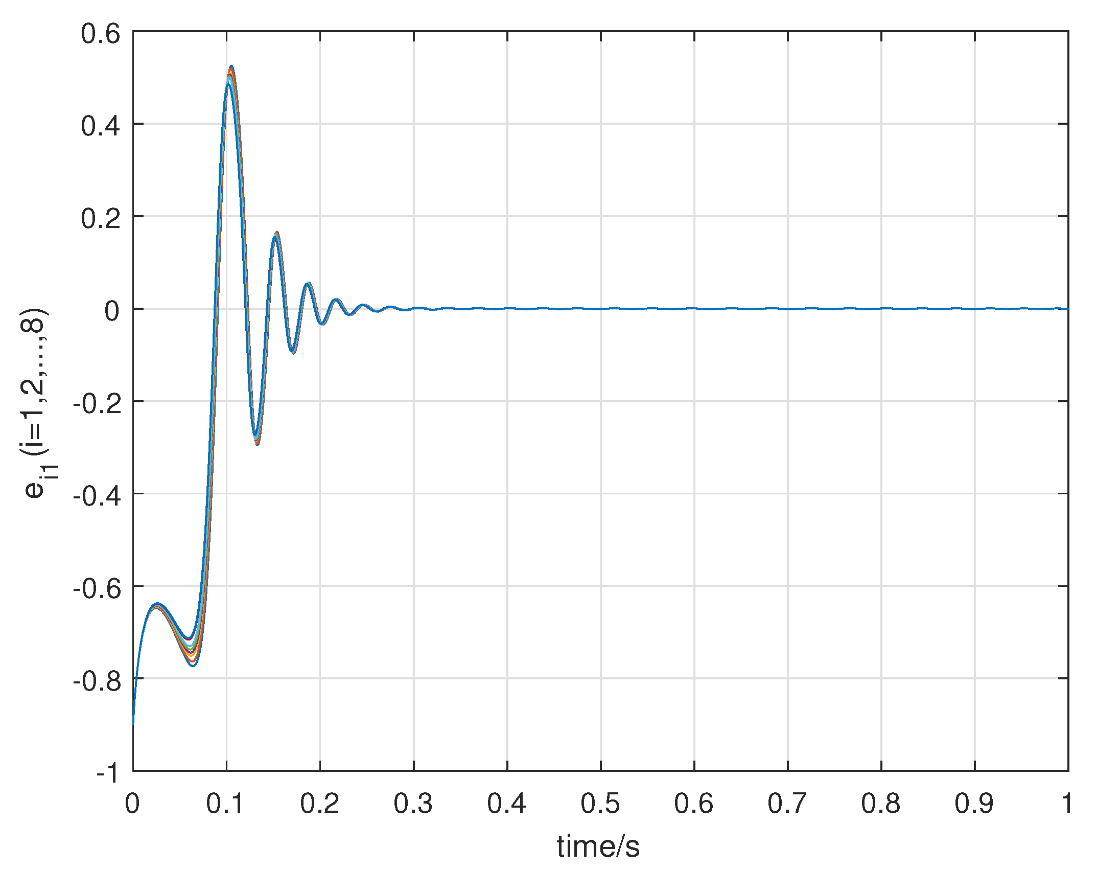
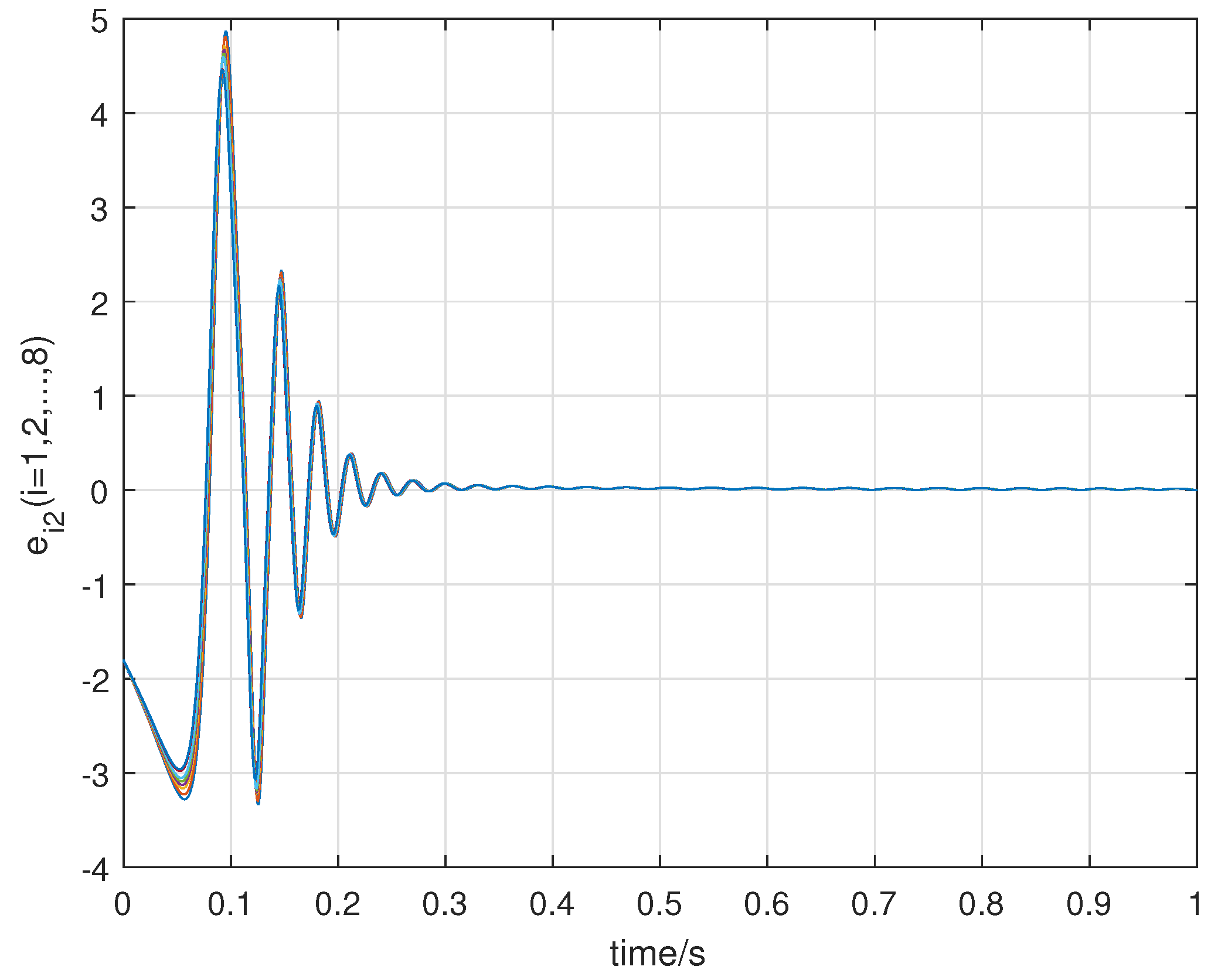
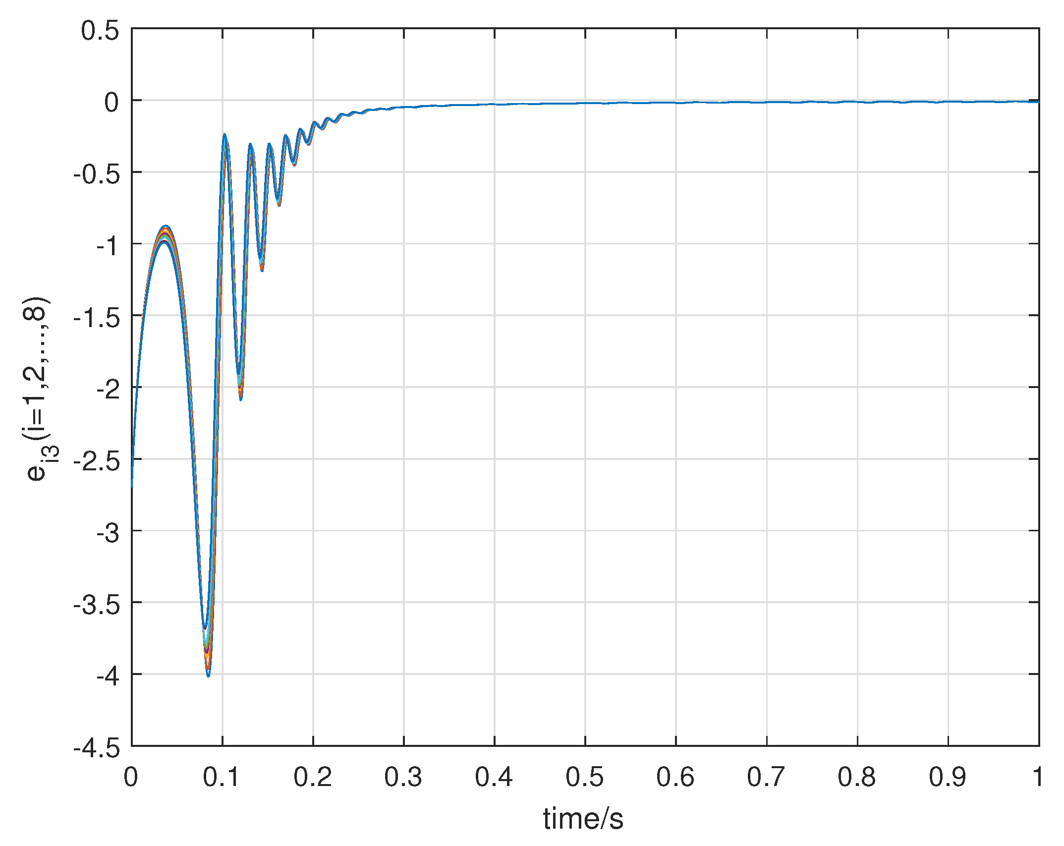
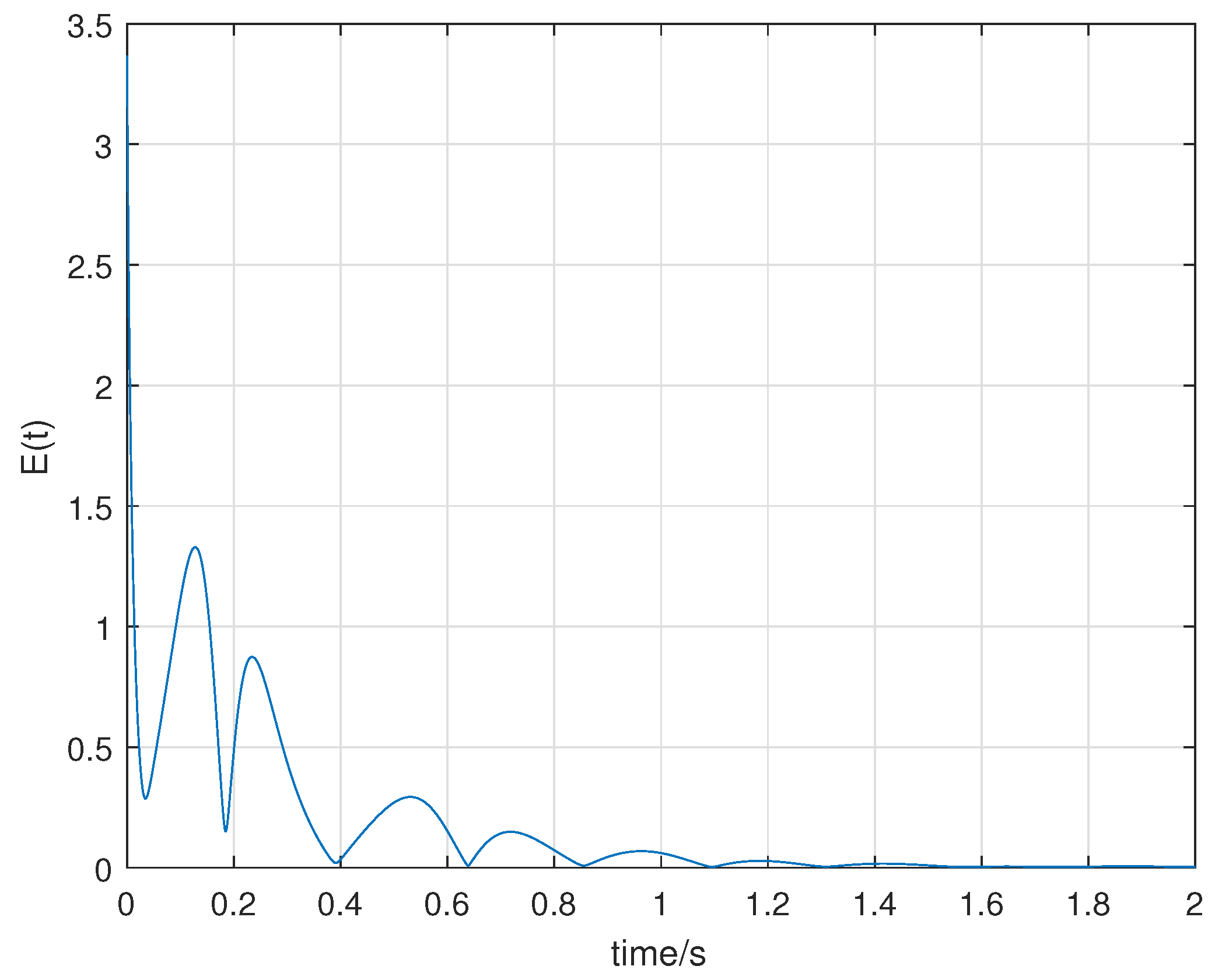
The control parameters are chosen as follows when we obtain the numerical simulation with software: the control matrix ${\mathit{K}}_j=kI(j=1,2,\cdots ,8)$, $k=50$ and the initial values ${\mathit{x}}_j\left(0\right)={(1+0.1\ast j,2+0.1\ast j,3+0.1\ast j)}^T,{\mathit{y}}_j\left(0\right)={(0.1+0.1\ast j,0.2+0.1\ast j,0.3+0.1\ast j)}^T(1\le j\le 8)$. The total synchronization error can be obtained by $E\left(t\right)=\sqrt{{\sum }_{j=1}^N(e_{j1}^2+e_{j2}^2+e_{j3}^2)/N}$. The results of numerical simulation are demonstrated as Figure 2, Figure 3, Figure 4 and Figure 5, which show the trajectories of synchronization errors $e_{j1}$, $e_{j2}$, $e_{j3}$, and $E\left(t\right)$ for the complex networks with eight fractional-order nodes wtih time variance. It follows from the simulation results and figures that the fractional-order error system is driven to the original point, i.e, the complex dynamical networks (70) and (73) with eight fractional-order nodes can achieve synchronization by the linear controller.

4.2. Synchronization of the Complex Dynamical Networks with 10 Fractional Order Nodes of teh Chaotic Lü System

Let us consider the complex networks be with 10 fractional-order nodes of chaotic Lü system [14,26,34]:

$$\begin{array}{cc}\hfill & {\mathrm{D}}_t^{\beta }{x}_{j1}=a(x_{j2}-x_{j1}),\hfill \\ & {\mathrm{D}}_t^{\beta }{x}_{j2}=b{x}_{j2}-x_{j1}{x}_{j3},\hfill \\ & {\mathrm{D}}_t^{\beta }{x}_{j3}=x_{j1}{x}_{j2}-c{x}_{j3},\hfill \end{array}$$

(75)

where $j=1,2,\cdots ,10$. If the fractional-order and the parameters are chosen as $a=36$, $b=20$, $c=3$, and $\beta =0.95$, respectively, the three-dimensional phase orbits of the fractional-order Lü chaotic system (75) is illustrated in Figure 5.

In the complex networks, we choose the coupling configuration matrix and the inner matrix of the complex dynamical networks with 10 fractional-order nodes of Lü chaotic system as follows:

$$p={\left(p_{ij}\right)}_{10\times 10}=\left(\begin{array}{cccccccccc}-4& 0& 1& 0& 0& 1& 0& 1& 0& 1\\ 0& -2& 0& 0& 1& 1& 0& 0& 0& 0\\ 1& 0& -5& 1& 1& 0& 1& 0& 1& 0\\ 0& 0& 1& -2& 0& 0& 0& 1& 0& 0\\ 0& 1& 1& 0& -5& 0& 1& 0& 1& 1\\ 1& 1& 0& 0& 0& -4& 0& 1& 0& 1\\ 0& 0& 1& 0& 1& 0& -3& 0& 0& 1\\ 1& 0& 0& 1& 0& 1& 0& -5& 1& 1\\ 0& 0& 1& 0& 1& 0& 0& 1& -3& 0\\ 1& 0& 0& 0& 1& 1& 1& 1& 0& -5\end{array}\right),A=\left(\begin{array}{ccc}1& 0& 0\\ 0& 1& 0\\ 0& 0& 1\end{array}\right).$$

The drive complex dyanmical networks with 10 fractional-order nodes of the Lü system are given as follows:

$$\begin{array}{c}\hfill {\mathrm{D}}_t^{\beta }{\mathit{x}}_j\left(t\right)=\mathit{f}\left({\mathit{x}}_j\left(t\right)\right)+\sum _{k=1}^N{p}_{jk}\mathit{A}{\mathit{x}}_k\left(t\right),j=1,2,\cdots ,10.\end{array}$$

(76)

which can be rewritten in the form (53):

$$\begin{array}{c}\hfill {\mathrm{D}}_t^{\beta }{\mathit{x}}_j\left(t\right)=\mathit{L}{\mathit{x}}_j\left(t\right)+\mathit{h}\left({\mathit{x}}_j\left(t\right)\right)+\sum _{k=1}^N{p}_{jk}\mathit{A}{\mathit{x}}_k\left(t\right),j=1,2,\cdots ,10,\end{array}$$

(77)

where

$$\mathit{L}=\left(\begin{array}{ccc}-a& a& 0\\ 0& b& 0\\ 0& 0& c\end{array}\right),$$

(78)

and

$$\mathit{h}\left({\mathit{x}}_j\left(t\right)\right)={(0,-x_{j1}{x}_{j3},x_{j1}{x}_{j2})}^T.$$

(79)

Adding the linear controller to the response complex networks with 10 fractional-order nodes of Lü system, we can obtain the following networks:

$${\mathrm{D}}_t^q{\mathit{y}}_j\left(t\right)=\mathit{L}{\mathit{y}}_j\left(t\right)+\mathit{h}\left({\mathit{y}}_j\left(t\right)\right)+\sum _{k=1}^N{p}_{jk}\mathit{A}{\mathit{y}}_k\left(t\right)-K_j({\mathit{y}}_j\left(t\right)-{\mathit{x}}_j\left(t\right)),j=1,2,\cdots ,10.$$

(80)

According to complex dynamical networks (77) and (80) with 10 fractional-order nodes, the controlled fractional error system is obtained as follows:

$$\begin{array}{c}\hfill {\mathrm{D}}_t^q{\mathit{e}}_j\left(t\right)=\mathit{L}{\mathit{e}}_j\left(t\right)+{\mathit{B}}_{x_j,y_j}{\mathit{e}}_j\left(t\right)+\sum _{k=1}^N{p}_{jk}\mathit{A}{\mathit{e}}_k\left(t\right)-K_j{\mathit{e}}_j\left(t\right),j=1,2,\cdots ,10,\end{array}$$

(81)

where ${\mathit{B}}_{x_j,y_j}(j=1,2,\cdots ,10)$ are bounded matrices with their elements depending on ${\mathit{x}}_j$ and ${\mathit{y}}_j$.

Since the fractional-order Lü system is chaotic, ${\mathit{x}}_j\left(t\right)(j=1,2,\cdots ,10)$ and ${\mathit{y}}_j\left(t\right)(j=1,2,\cdots ,10)$ are bounded. It can easily be obtained that ${\mathit{e}}_j^T\left(t\right){\mathit{B}}_{{\mathit{x}}_j,{\mathit{y}}_j}{\mathit{e}}_j\left(t\right)=-x_{j3}{e}_{j1}{e}_{j2}+x_{j2}{e}_{j1}{e}_{j3}\le 30{\mathit{e}}_j^T\left(t\right){\mathit{e}}_j\left(t\right)$ by calculating the eigenvalue of maximum, which implies $m\approx 30$. According to Corollary 2, if the matrices $S_j=\frac{L^T+L}{2}+(m-k)I$ ($j=1,2,\cdots ,10$) are all negative positive matrices, the fractional-order error system (74) is asymptotically stable, i.e., the complex networks (77) and (80) with 10 fractional order nodes of the Lü system can achieve synchronization. The maximal eigenvalue of matrix $\frac{L^T+L}{2}$ can be obtained as ${\lambda }_{max}\approx 25$ easily. Hence, if the all control parameters ${\mathit{k}}_j(j=1,2,\cdots ,10)$ satisfy the conditions of Theorem 1, the complex dynamical networks (77) and (80) with 10 fractional-order nodes of Lü system can achieve synchronization by the linear controllers.

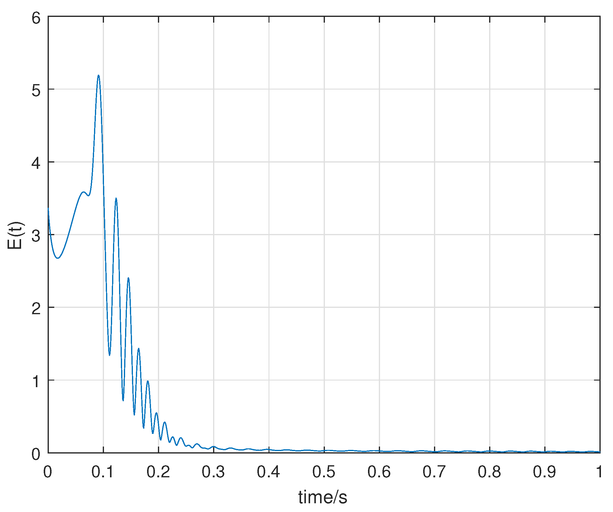
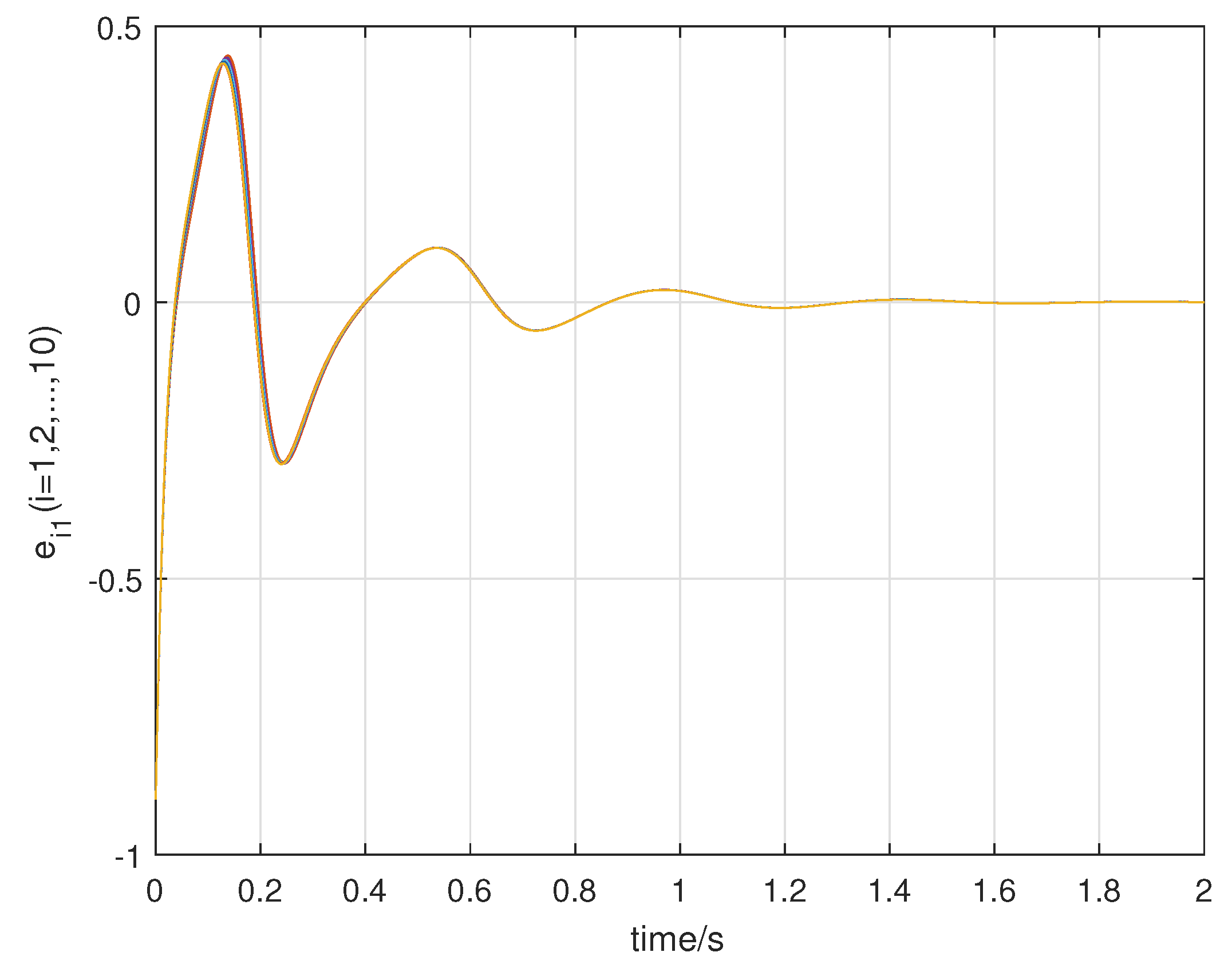
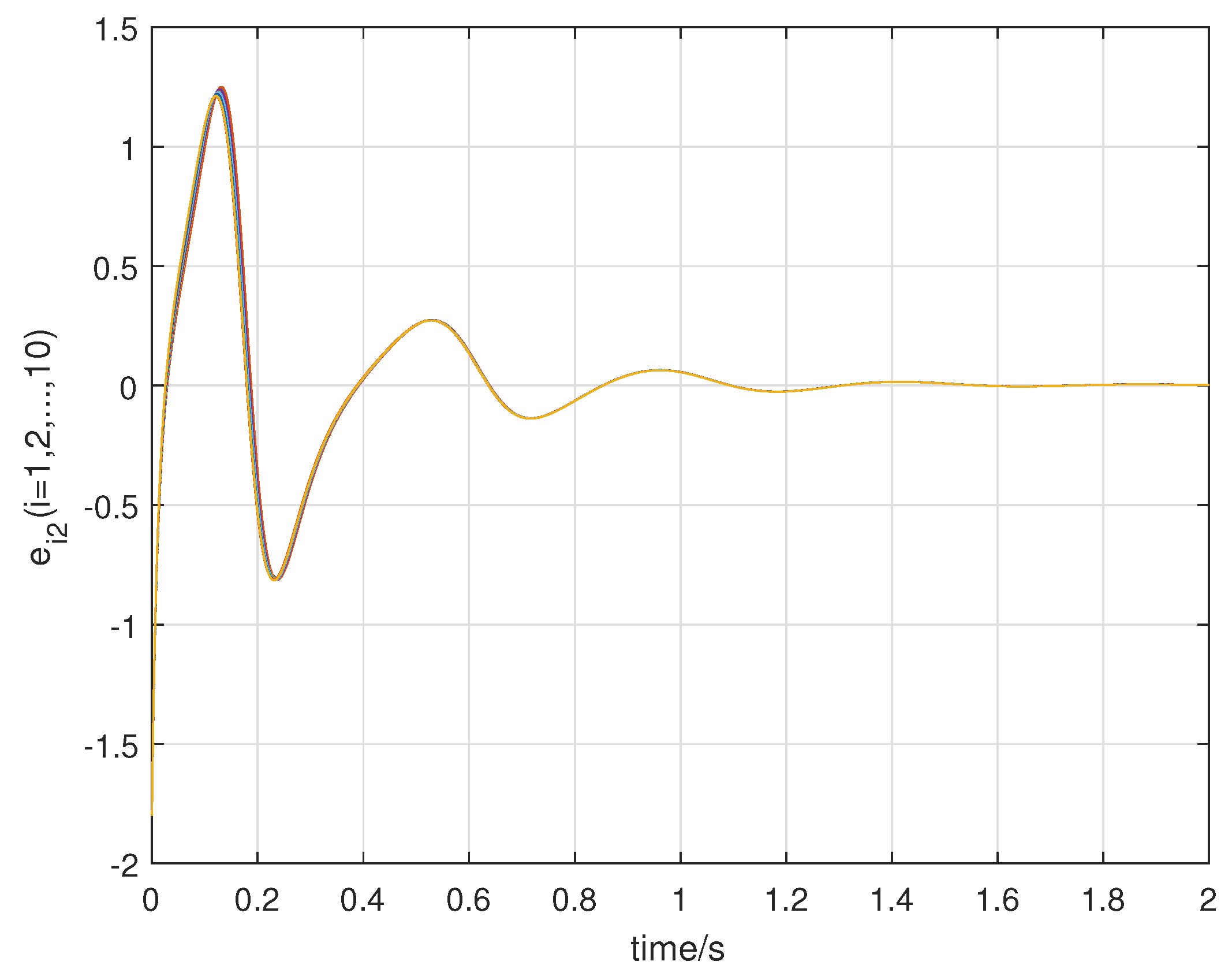
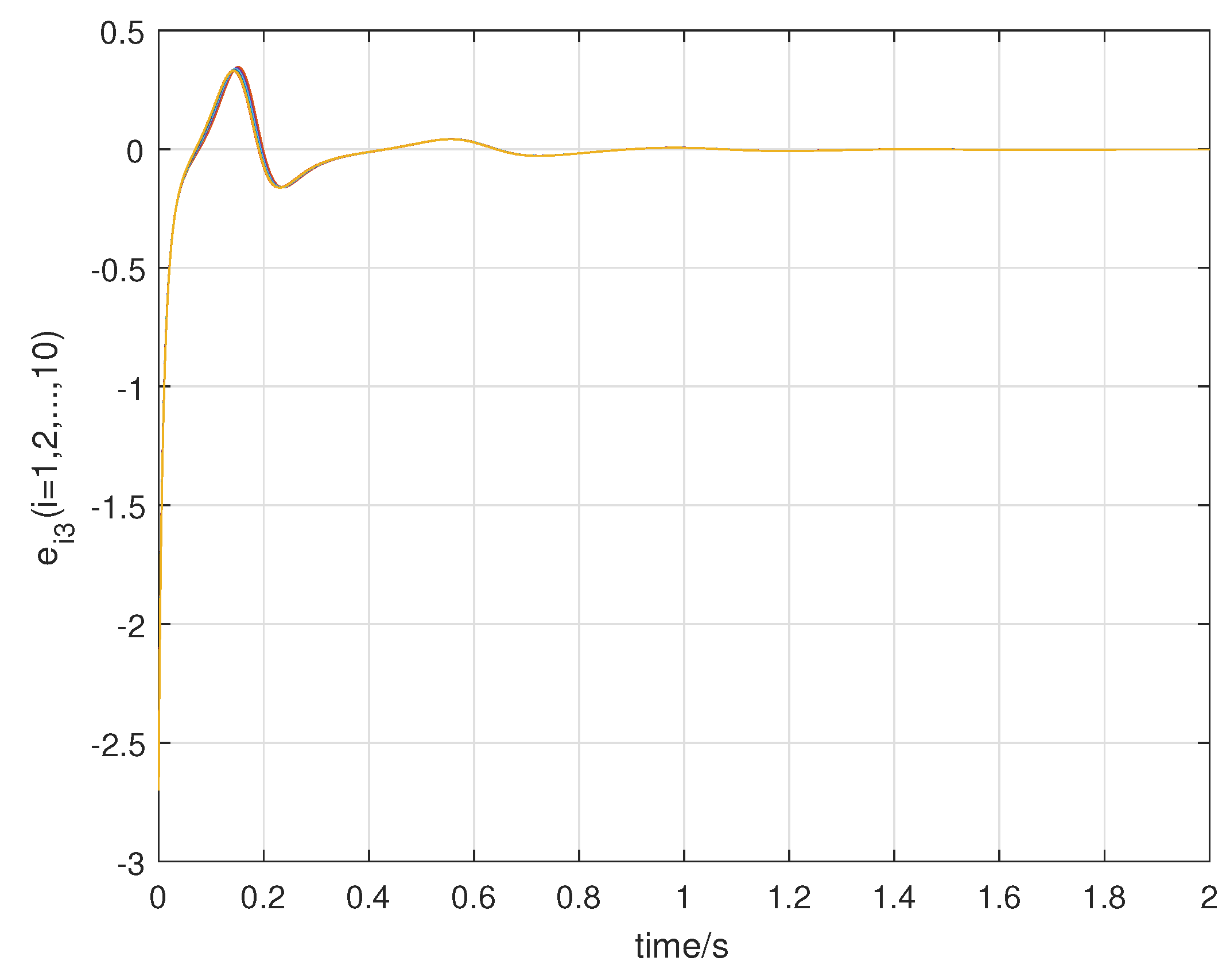
The control parameters are chosen as follows when we obtain the numerical simulation with software: the control matrix is ${\mathit{\omega }}_j=I(j=1,2,\cdots ,10)$, ${\mathit{k}}_j=60\ast I(j=1,2,\cdots ,10)$, and the initial values are ${\mathit{x}}_j\left(0\right)={(1-0.1\ast j,2-0.1\ast j,3-0.1\ast j)}^T,{\mathit{y}}_j\left(0\right)={(0.1+0.1\ast j,0.2+0.1\ast j,0.3+0.1\ast j)}^T(1\le j\le 10)$. The results of the numerical simulation are demonstrated in Figure 6, Figure 7, Figure 8 and Figure 9, which show the trajectories of the errors $e_{j1}$, $e_{j2}$, $e_{j3}$, and $E\left(t\right)$ for the complex networks with 10 fractional-order nodes with time variance. It follows from the simulation results and figures that the fractional-order error system is driven to original point, i.e., the complex networks (77) and (80) with 10 fractional-order nodes of the Lü system can achieve synchronization by the linear controller.

5. Conclusions

In conclusion, we proposed the synchronization of complex dynamical networks with fractional-order chaotic nodes via a simple Lyapunov function. Some new sufficient synchronization methods are proposed based on the Lyapunov stability theory and a simple Lyapunov function. These methods can apply to arbitrary complex dynamics with fractional-order nodes, which indicates that these methods are more general and effective than others. The results of the numerical simulations for two complex networks with fractional-order nodes demonstrate the universality and the effectiveness of the proposed method. We have implemented and verified our method for fractional-order complex networks with other chaotic systems [33,34,36,43,44], such as the fractional-order Newton–Leipnik system [36], the fractional-order Chen system [33], the fractional-order modified coupled dynamos system [43], the fractional-order Arneodo system [44], etc. The results of numerical simulation show that the complex networks with fractional-order nodes of any chaotic system can be achieved to synchronize effectively and fast by the proposed linear controller. On the other hand, we study the synchronization of fractional-order complex networks with different number of nodes. In our laptop, the maximum of the nodes is about 50. It needs more time to give the numerical solution and achieve the synchronization.

In the future work, we will consider that how to extend our method to other complex networks such as weighted networks and how to widen the method to the larger complex networks. Finally, we will study how to apply our method to real complex networks.

References

- Strogatz, S.H. Exploring comples networks. Nature 2001, 410, 268–276. [Google Scholar] [CrossRef] [PubMed] [Green Version]
- Albert, R.; Barabási, A.L. Statistical mechanics of comples networks. Rev. Mod. Phys. 2002, 74, 47–97. [Google Scholar] [CrossRef] [Green Version]
- Wang, X.; Chen, G.R. Complex network: Small-world, scale-free and beyond. IEEE Circuits Syst. Mag. 2003, 3, 6–20. [Google Scholar] [CrossRef] [Green Version]
- Bellingeri, M.; Vincenzi, S. Robustness of empirical food webs with varying consumer’s sensitivities to loss of resources. J. Theor. Biol. 2016, 333, C18–C26. [Google Scholar] [CrossRef]
- Pandit, S.A.; Amritkar, R.E. Characterization and control of small-wold network. Phys. Rev. E 1999, 60, 1119–1122. [Google Scholar] [CrossRef] [Green Version]
- Lü, J.H.; Chen, G.R. A time-varying complex dynamical network models and its controlled synchronization criteria. IEEE Trans. Auto. Contr. 2005, 50, 841–846. [Google Scholar]
- Zhou, J.; Lu, J.; Lü, J.H. Adaptive Synchronization of an uncertain complex dynamical network. IEEE Trans. Autom. Control. 2006, 51, 652–656. [Google Scholar] [CrossRef] [Green Version]
- Wang, X.; Chen, G.R. Synchronization in small-world dynamical networks. Int. J. Bifurc. Chaos 2002, 12, 187–192. [Google Scholar] [CrossRef]
- Wu, C. Synchronization in arrays of coupled nonlinear systems with delay and nonreciprocal time-varying couping. IEEE Trans. Circuits Syst. II 2005, 52, 282–286. [Google Scholar]
- Yu, W.; Cao, J.; Lü, J.H. Global synchronization of linearly hybrid coupled networks with time-varying delay. Siam J. Appl. Dyn. Syst. 2008, 7, 108–133. [Google Scholar] [CrossRef]
- Cao, J.; Li, P.; Wang, W. Global synchronization in arrays of delayed neural networks with constant and delayed coupling. Phys. Lett. 2006, 353, 318–325. [Google Scholar] [CrossRef]
- Tang, Y.; Gao, H.J.; Kurths, J. Distributed robust synchronization of dynamical networks with stochastic coupling. IEEE Trans. Circuits Syst. Regul. Pap. 2014, 61, 1508–1519. [Google Scholar] [CrossRef]
- Podlubny, I. Fractional Differential Equations; Academic Press: San Diego, CA, USA, 1999. [Google Scholar]
- Petras, I. Fractional-Oorder Nonlinear Systems: Modeling, Analysis and Simulation; Higher Education Press: Beijing, China, 2011. [Google Scholar]
- Koeller, R.C. Polynomial operators, Stieltjes convolution, and fractional calculus in hereditary mechanics. Acta Mech. 1986, 58, 251–264. [Google Scholar] [CrossRef]
- Grigorenko, I.; Grigorenko, E. Chaotic Dynamics of the Fractional Lorenz System. Phys. Rev. Lett. 2003, 91, 034101. [Google Scholar] [CrossRef] [PubMed]
- Hartley, T.T.; Lorenzo, C.F.; Qammer, H.K. Chaos on a fractional Chua’s system. IEEE Trans. Circuits Syst. I 1995, 42, 485–790. [Google Scholar] [CrossRef]
- Li, C.G.; Chen, G.R. Chaos in the fractional-order Chen system and its control. Chaos Solitons Fractals 2005, 22, 549–554. [Google Scholar] [CrossRef]
- Wang, J.W.; Zhang, Y.B. Network synchronization in a population of star-coupled fractional nonlinear oscillators. Phys. Lett. A 2010, 374, 1464–1468. [Google Scholar] [CrossRef]
- Tang, Y.; Wang, Z.; Fang, J. Ping control of fractional-order weighted complex networks. Chaos 2009, 19, 013112. [Google Scholar] [CrossRef]
- Wu, X.J.; Lu, H.T. Outer synchronization between two different fractional-order general complex dynamical networks. Chin. Phys. D 2010, 19, 070511. [Google Scholar]
- Delshad, S.S.; Asheghan, M.M.; Beheshti, M.H. Synchronization of N-coupled incommensurate fractional-order chaotic systems with ring connection. Commun. Nonlinear Sci. Numer. Simul. 2011, 16, 3815–3824. [Google Scholar] [CrossRef]
- Asheghan, M.M.; Miguez, J.; Mohammad, T.H.B.; Tavazoei, M.S. Robust outer synchronization between two complex networks with fractional-order dynamics. Chaos 2011, 21, 033121. [Google Scholar] [CrossRef] [PubMed] [Green Version]
- Zhang, R.F.; Chen, D.Y.; Do, Y.; Ma, X.Y. Synchronization and anti-synchronization of fractional dynamical networks. J. Vib. Control. 2015, 21, 3383–3402. [Google Scholar] [CrossRef]
- Wang, Y.; Li, T.Z. Synchronization of fractional-order complex dynamical networks. Phys. Stat. Mech. Its Appl. D 2015, 428, 1–12. [Google Scholar] [CrossRef]
- Yang, Y.; Wang, Y.; Li, T.Z. Outer synchronization of fractional-order complex dynamical networks. Optik 2016, 127, 7395–7407. [Google Scholar] [CrossRef]
- Lü, L.; Li, C.; Chen, L. Outer synchronization between uncertain networks with adaptive scaling function and different node numbers. Phys. A 2018, 506, 909–918. [Google Scholar] [CrossRef]
- Du, H. Adaptive open-plus-closed-loop control method of modified function projective synchronization in complex networks. Int. J. Mod. Phys. C 2011, 22, 1393–1407. [Google Scholar] [CrossRef]
- Gorenflo, R.; Mainardi, F.; Moretti, D.; Paradisi, P. Time fractional diffusion: A discrete random walk approach. Nonlinear Dyn. 2002, 29, 129–143. [Google Scholar] [CrossRef]
- Yuste, S.; Murillo, J. On three explicit difference schemes for fractional diffusion and diffusion-wave equations. Phys. Scr. 2009, 136, 14–25. [Google Scholar]
- Li, Y.; Chen, Y.; Podlubny, I. Stability of fractional-order nonlinear dynamic systems: Lyapunov direct method and generalized Mittag Leffler stability. Comput. Math. Appl. 2010, 59, 1810–1821. [Google Scholar] [CrossRef] [Green Version]
- Slotine, J.J.; Li, W. Applied Nonlinear Control; Prentice Hall: Hoboken, NJ, USA, 1999. [Google Scholar]
- Li, T.Z.; Wang, Y.; Yong, Y. Designing synchronization schemes for fractional-order chaoticsystem via a single state fractional-order controller. Optik 2014, 125, 6700–6705. [Google Scholar] [CrossRef]
- Li, T.Z.; Wang, Y.; Luo, M.K. Control of fractional chaotic and hyperchaotic systems based on a fractional-order controller. Chin. Phys. B 2014, 23, 080501. [Google Scholar] [CrossRef]
- Wang, X.J.; Li, J.; Chen, G.R. Chaos in the fractional-order unified system and its synchronization. J. Frankl. Inst. 2008, 345, 392–401. [Google Scholar]
- Sheu, L.J.; Chen, H.K.; Chen, J.H.; Tam, L.M.; Chen, W.C.; Lin, K.T.; Kang, Y. Chaos in the newton-leipnik system with fractional-order. Chaos Solitons Fractals 2008, 36, 98–103. [Google Scholar] [CrossRef]
- Huang, X.; Cao, X.; Ma, Y. Sampled-data exponential synchronization of complex dynamical networks with time-varying delays and TCS fuzzy nodes. Comput. Appl. Math. 2022, 41, 74. [Google Scholar] [CrossRef]
- Zhu, S.; Zhou, J.; Yu, X. Bounded Synchronization of Heterogeneous Complex Dynamical Networks: A Unified Approach. IEEE Trans. Autom. Control 2021, 66, 1756–1762. [Google Scholar] [CrossRef]
- Peng, C.C.; Zhang, W.H. Linear feedback synchronization and anti-synchronization of a class of fractional-order chaotic systems based on triangular structure. Eur. Phys. J. Plus 2019, 134, 292. [Google Scholar] [CrossRef]
- Agrawal, S.K.; Srivastava, M.; Das, S. Synchronization of fractional-order chaotic systems using active control method. Chaos Solitons Fractals 2012, 45, 737–752. [Google Scholar] [CrossRef]
- Shi, L.; Zhu, H.; Zhong, S. Cluster synchronization of linearly coupled complex networks via linear and adaptive feedback pinning controls. Nonlinear Dyn. 2017, 88, 859–870. [Google Scholar] [CrossRef]
- Shi, L.; Zhang, C.; Zhong, S. Synchronization of singular complex networks with time-varying delay via pinning control and linear feedback control. Chaos Solitons Fractals 2021, 145, 110805. [Google Scholar] [CrossRef]
- Wang, X.Y.; He, Y.J.; Wang, M.J. Chaos control of a fractional-order modified coupled dynamos system. Nolinear Anal. 2009, 71, 6126–6134. [Google Scholar] [CrossRef]
- Chen, L.P.; Chai, Y.; Wu, R.C.; Sun, J.; Ma, T.D. Cluster synchronization in fractional-order complex dynamical networks. Phys. Lett. A 2012, 376, 2381–2388. [Google Scholar] [CrossRef]
Figure 1.
The three-dimensional phase orbits for fractional order chaotic Liu system with the order .
Figure 2.
Trajectories of synchronization errors for the complex networks (70) and (73) with eight fractional order nodes with time variance.
Figure 3.
Figure 4.
Figure 5.
Trajectories of total synchronization errors for the complex networks (70) and (73) with eight fractional order nodes with time variance.
Figure 6.
Trajectories of synchronization errors for the complex networks (77) and (80) with 10 fractional order nodes with time variance.
Figure 7.
Figure 8.
Publisher’s Note: MDPI stays neutral with regard to jurisdictional claims in published maps and institutional affiliations. |
© 2022 by the authors. Licensee MDPI, Basel, Switzerland. This article is an open access article distributed under the terms and conditions of the Creative Commons Attribution (CC BY) license (https://creativecommons.org/licenses/by/4.0/).
Share and Cite
MDPI and ACS Style
Zhang, Y.; Li, T.; Zhang, Z.; Wang, Y. Novel Methods for the Global Synchronization of the Complex Dynamical Networks with Fractional-Order Chaotic Nodes. Mathematics 2022, 10, 1928. https://0-doi-org.brum.beds.ac.uk/10.3390/math10111928
AMA Style
Zhang Y, Li T, Zhang Z, Wang Y. Novel Methods for the Global Synchronization of the Complex Dynamical Networks with Fractional-Order Chaotic Nodes. Mathematics. 2022; 10(11):1928. https://0-doi-org.brum.beds.ac.uk/10.3390/math10111928
Chicago/Turabian StyleZhang, Yifan, Tianzeng Li, Zhiming Zhang, and Yu Wang. 2022. "Novel Methods for the Global Synchronization of the Complex Dynamical Networks with Fractional-Order Chaotic Nodes" Mathematics 10, no. 11: 1928. https://0-doi-org.brum.beds.ac.uk/10.3390/math10111928
Note that from the first issue of 2016, this journal uses article numbers instead of page numbers. See further details here.