
Wind Speed Prediction via Collaborative Filtering on Virtual Edge Expanding Graphs
by
 , ,
, ,
Xiang Ying
1,2,3,4, 
Keke Zhao
4,
Zhiqiang Liu
1,2,3,
Jie Gao
1,2,3,
Dongxiao He
1,
Xuewei Li
1,2,3 and
Wei Xiong
5,* 1
College of Intelligence and Computing, Tianjin University, Tianjin 300072, China
2
Tianjin Key Laboratory of Cognitive Computing and Application, Tianjin 300350, China
3
Tianjin Key Laboratory of Advanced Networking, Tianjin 300350, China
4
Tianjin International Engineering Institute, Tianjin University, Tianjin 300072, China
5
TCU School of Civil Engineering, Tianjin Chengjian University, Tianjin 300384, China
*
Author to whom correspondence should be addressed.
Mathematics 2022, 10(11), 1943; https://0-doi-org.brum.beds.ac.uk/10.3390/math10111943
Submission received: 11 April 2022
/
Revised: 15 May 2022
/
Accepted: 21 May 2022
/
Published: 6 June 2022
(This article belongs to the Special Issue Mathematics-Based Methods in Graph Machine Learning)
Abstract
:Accurate and stable wind speed prediction is crucial for the safe operation of large-scale wind power grid connections. Existing methods are typically limited to a certain fixed area when learning the information of the wind speed sequence, which cannot make full use of the spatiotemporal correlation of the wind speed sequence. To address this problem, in this paper we propose a new wind speed prediction method based on collaborative filtering against a virtual edge expansion graph structure in which virtual edges enrich the semantics that the graph can express. It is an effective extension of the dataset, connecting wind turbines of different wind farms through virtual edges to ensure that the spatial correlation of wind speed sequences can be effectively learned and utilized. The new collaborative filtering on the graph is reflected in the processing of the wind speed sequence. The wind speed is preprocessed from the perspective of pattern mining to effectively integrate various information, and the k-d tree is used to match the wind speed sequence to achieve the purpose of collaborative filtering. Finally, a model with long short-term memory (LSTM) as the main body is constructed for wind speed prediction. By taking the wind speed of the actual wind farm as the research object, we compare the new approach with four typical wind speed prediction methods. The mean square error is reduced by 16.40%, 11.78%, 9.57%, and 18.36%, respectively, which demonstrates the superiority of the proposed new method.
Keywords:
wind speed prediction; virtual edge expanding graphs; collaborative filtering; pattern mining; LSTM networkMSC:
68T071. Introduction
Climate change and energy issues are currently prominent global challenges. In recent years, it has become a global trend to generate electricity from renewable energy rather than traditional fossil energy. As an important green renewable energy, wind energy has developed rapidly under this trend [1]. However, wind power generation is unstable due to the inherent volatility, indirectness, and low energy density of wind energy resources. Therefore, accurate wind speed prediction is of great significance to the stable power generation and dispatching of power [2].
As a time series, wind speed can generally be divided into point forecasting and probabilistic forecasting. Among these, the wind speed probability prediction includes interval prediction and density prediction [3], and different methods can be selected according to the prediction target. The existing wind speed prediction methods can be divided into three categories according to the modeling mechanism: physical methods [4], statistical methods [5], and machine learning methods [6]. The physical method mainly predicts the wind speed according to the changing laws of some physical properties that cause wind speed fluctuations [7]. The most typical is the model based on numerical weather prediction (NWP) [8]. Statistical methods describe the nonlinear relationship between wind speed and power, such as the autoregressive moving average model (ARMA) [9], the autoregressive integrated moving average model (ARIMA) [10], the Kalman filter [11], and the Markov model [12], by analyzing the statistical laws of historical wind speed data, at the same time, avoid physical factors that cannot be adequately and precisely described. However, for multiple time series, such as wind speed, physical methods and statistical methods cannot be well modeled and predicted, and the effect of using machine learning models will be much better. Machine learning methods mainly use artificial intelligence algorithms to describe the highly complex nonlinear relationship between input data and output data. They mainly include support vector regression (SVR) [13], k-nearest neighbor algorithm (KNN) [14], and multi-layer perceptron (MLP) [15]. In addition, a combination of these models can also be used, such as Markov random fields, based on Markov models and the Bayesian theory, which can be used to solve many problems in the field of machine learning [16]. These methods are studied from different angles in an attempt to make accurate predictions of wind speed. However, due to the unavoidable influence of physical factors and the failure to fully exploit the spatiotemporal characteristics of wind speed when using and processing wind speed data, the accuracy of wind speed prediction is difficult to improve.
In order to solve the above problems and effectively extract the spatiotemporal features of wind speed, this paper proposes a wind speed prediction method based on a virtual edge expansion graph and a collaborative filtering algorithm. Wind speed is affected by nature, and there are different degrees of spatial correlation and temporal correlation. Therefore, in this paper, the selection of the wind speed dataset is not limited to a certain fixed area, and considers the characteristics of the wind speed sequence, then implements an effective feature extraction strategy for the collected data. The dataset used in this paper is from the National Renewable Energy Laboratory (NREL) (https://www.nrel.gov (accessed on 8 December 2021)), and the results show that the accuracy of the proposed method is higher than that of some popular machine learning methods. The contributions of this paper are as follows:
- Aiming at the problem that the datasets used for wind speed prediction often come from the wind turbine to be predicted and the surrounding wind turbines, this paper proposes to extend the meaning of the actual edge, build a virtual edge to connect wind turbines in different areas, and enhance usage dataset size.
- In view of the problem that the spatiotemporal features extracted in wind speed prediction are not sufficient, this paper proposes to use the collaborative filtering algorithm to preprocess the wind speed sequence from the perspective of pattern mining and matching, and then use k-d tree to match the wind speed pattern to effectively extract and integrate the wind speed information.
- For the proposed new wind speed prediction method, this paper constructs a model with LSTM network as the main body, then evaluates the performance of the model through mean square error and root mean square difference, comparing it with some popular wind speed prediction methods. Experiments show that the use of a virtual edge expansion graph and a collaborative filtering algorithm is beneficial to the improvement of the wind speed prediction effect.
2. Related Work
2.1. Common Methods
For the wind speed prediction problem, the performance of traditional models can no longer meet the requirements of high precision. In recent years, more and more researchers have turned their attention to deep learning. Deep learning models with high nonlinearity and strong generalization ability have great advantages over traditional methods in improving the accuracy of wind speed prediction. Commonly used deep learning models include the use of the recurrent neural network (RNN) [17], long short-term memory network [18], convolutional neural network(CNN) [19], graph convolutional neural network [20], and so on. These models have many successful applications in time series forecasting problems [21,22,23]. For example, Peng et al. [24] proposed a novel spatiotemporal correlation dynamic graph neural network framework, which samples short-term, medium-term and long-term historical passenger flow data, respectively, and learns the topology of the urban transportation network and the spatiotemporal feature representation of transportation hubs to predict urban traffic passenger flow. Currently, the focus of wind speed prediction research efforts is to improve the learning ability of these models in order to better capture wind speed characteristics. In recent years, most of the literature has improved from the aspects of data preprocessing and the combination model.
Since the wind speed series is a non-stationary time series, it contains a lot of noise, which may interfere with the learning and prediction of the model. At the same time, many methods do not fully consider the spatiotemporal correlation of the wind speed series when forecasting wind speed. Therefore, it is necessary to preprocess the wind speed sequence. At present, there are two typical methods for wind speed data preprocessing. One is to construct a two-dimensional wind speed feature image, map the wind turbine to a two-dimensional plane, and generate a series of pictures containing wind speed information in time sequence, which not only reflects the temporal characteristics of wind speed, but also retains the spatial characteristics of wind speed; for example, Lilin Cheng et al. [25] proposed a new method for short-term wind power prediction based on image input and an enhanced convolutional network and achieved high-precision results. The second is to use the signal decomposition method to decompose the wind speed time series. The mainstream methods include wavelet transform [26], empirical mode decomposition [27], and variational mode decomposition [28], etc., For example, Yaoran Chen et al. [29] used ensemble empirical mode decomposition(EEMD) to divide the original wind sequence into several intrinsic mode functions to form a potential feature set for prediction, and obtained good results. In addition to the decomposition method, data processing methods such as clustering [30] and dimensionality reduction [31] can also be used to preprocess the wind speed series to reduce the number and dimensions of data for tasks such as predictive modeling and decision support.
When a single model is used for wind speed prediction, the prediction accuracy that can be achieved is very limited and cannot meet the actual requirements. Therefore, some researchers have proposed a method for combining models, which combines the advantages of different models and effectively improves the prediction accuracy. For example, Qiaomu Zhu et al. [32] proposed a unified framework integrating CNN and LSTM. Experiments show that the combined model has better prediction accuracy than the single model. In addition, optimization algorithms, such as batch gradient descent [33], momentum [34], Adam [35], etc., can also be used to improve the training efficiency of the model, or to optimize the hyperparameters of the model. These methods first use a large amount of historical wind speed data to train the model, and then use the trained model to make predictions. In essence, they are all mining and matching patterns of wind speed sequences. From this perspective, the wind speed prediction problem can be regarded as a pattern mining and matching problem.
2.2. Collaborative Filtering
The collaborative filtering algorithm [36] is a common method for mining data patterns, which is generally used in recommender systems, using the historical records related to users and items for recommendation. Researchers have conducted in-depth research on collaborative filtering algorithms and proposed many methods, such as neighborhood-based methods, latent semantic models, and graph-based random walk algorithms [37]. Among these methods, the most widely used is the neighborhood-based method. Neighborhood-based collaborative filtering methods fall into two categories: user-based collaborative filtering and item-based collaborative filtering.
User-based collaborative filtering is employed to find users who are similar to user u among all users, and then use these neighboring users are utilized to average or weight the ratings of item i to obtain the predicted value. This process can be expressed as:
Item-based collaborative filtering is employed to find nearby items i that are similar to the predicted item, and then utilized to find the average rating of these neighbors by user u. It can be calculated by the following formula:
When the number of items in the system is much smaller than the number of users, it is better to choose the item-based collaborative filtering method. On the contrary, if the flow of items in the system is relatively large, it is better to choose the user-based collaborative filtering method.
k-d tree [38] is a way to implement collaborative filtering algorithm. k-d tree is a tree-like data structure that stores instance points in k-dimensional space for fast retrieval. It is mainly used for similarity retrieval in high-dimensional space, and finding the nearest points in multiple dimensions for matching. In fact, k-d tree is a binary search tree; each node corresponds to a hyperrectangle of multidimensional space. The construction of k-d tree is a recursive process. Each time a dimension is selected for division, the k-dimensional space and the data set are divided into two parts, and so on, until the space contains only one data point. This special construction process also makes the querying of k-d trees very fast and efficient. According to the method of establishing data index by k-d tree, only one dimensional value in multi-dimensional spaces needs to be processed each time, which is relatively simple. In addition, the k-d tree alternately detects the values of different attributes, which can narrow the search range to the nodes containing the query results more quickly.
2.3. Wind Farm Graph
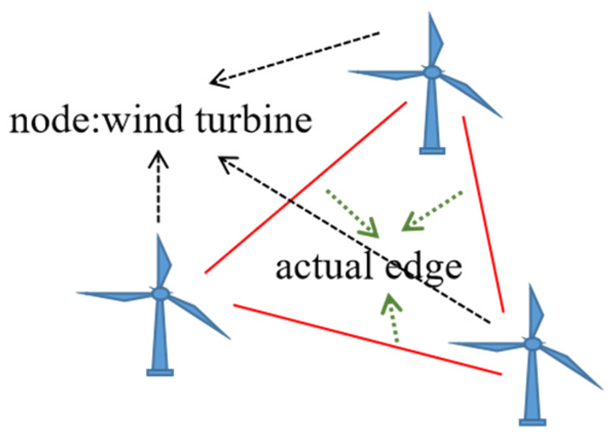
We know that for any wind turbine in a wind farm, it can be scaled down and mapped on a two-dimensional plane according to the latitude and longitude, and then a two-dimensional plan of the wind farm can be drawn according to the relative positional relationship between the wind turbines. In fact, this is a method of graph representation learning [39]. Among them, each wind turbine is a node of this graph, and the straight line connecting the wind turbines is the edge of the graph. In this paper, the edge connecting the wind turbines of the same wind farm is called the actual edge, which can describe the specific position relationship of the wind turbines, as shown in Figure 1. This graph representation of the learning method is the basis of the virtual edge extension graph proposed in this paper.
3. Method
At present, a large number of researches on wind speed prediction focus on methods based on deep learning; its network structure is flexible and has strong nonlinear fitting ability. The calculation process of the deep learning model is actually a function fitting, which forms a certain mapping between the input and the output, and directly describes the relationship between the two. However, wind, as a result of air movement, is a fluid. In fluid mechanics, laminar flow and turbulent flow are two properties of fluid flow. Laminar flow means that the fluid particles move forward uniformly, the trajectory presents a regular smooth curve, and the fluid particles do not interfere with each other. Turbulence means that some fluid particles acquire a considerable velocity component perpendicular to the flow direction, resulting in a random flow of the fluid in any cross-section. Although the whole is still flowing forward, it is in a chaotic state. Turbulence is created as the wind passes over both types of surfaces, forming branches of different sizes and directions. In this case, if only the deep learning model is used, it is impossible to fit all the wind components; therefore, the model cannot learn the wind speed information well, thus affecting the accuracy of wind speed prediction.
Based on this angle, in order to solve the problem that the data source for wind speed prediction is limited to a fixed area, and the mining of the spatiotemporal correlation of the wind speed series is not enough, this paper proposes a wind speed prediction method based on a virtual edge expanded graph and a collaborative filtering algorithm. From the two aspects of expanding the size of the wind speed data set and effectively extracting the spatiotemporal features of the wind speed sequence, the accuracy of wind speed prediction is effectively improved.
3.1. Virtual Edge Expansion Graph
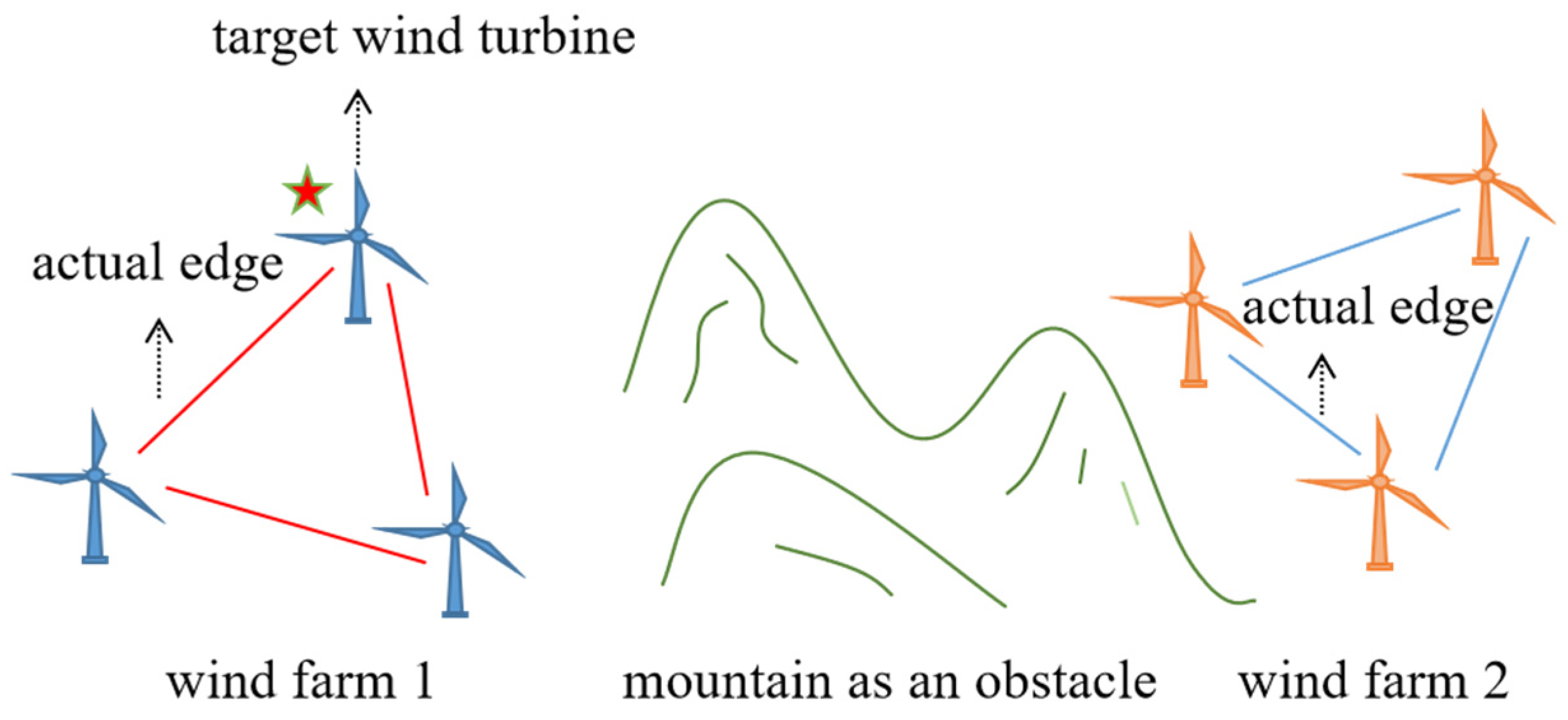
We noticed that the existing wind speed prediction methods are conservative in the use of datasets, and can be basically divided into two categories: one is to use the historical wind speed data of the wind turbine to be predicted; the other is to use the historical wind speed data of the wind turbines adjacent to the wind turbine to be predicted. As shown in Figure 2, for the target wind turbine, the wind speed dataset used is generally derived from the adjacent wind turbines in the same wind farm (wind farm 1) connected by the actual edge, while the wind turbine data of other wind farms (wind farm 2) are not collected. Because wind farm 2 and the target wind turbine are blocked by the mountain, the correlation between the wind speed sequence of its wind turbine and the wind speed sequence of the target wind turbine is generally small.
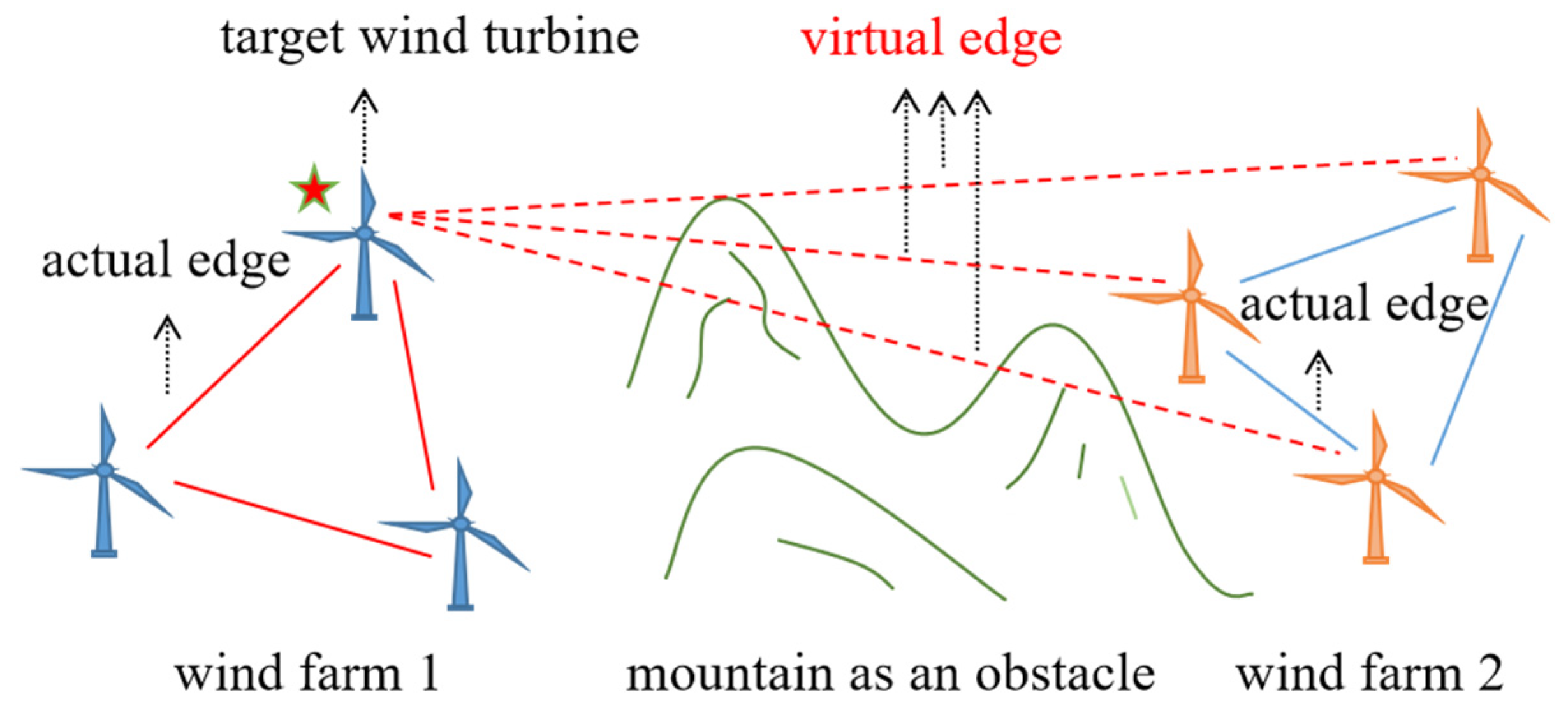
However, with the changes of meteorological and geographical factors, the wind speed series of wind farms in different regions may intersect and show similar changing trends. Therefore, we believe that there may be similarities between the sequences of different wind turbines, and the dataset used for wind speed prediction does not have to be limited to a single turbine, nor to a fixed area around the wind turbine to be predicted. Moreover, the wind farm graph does not have to be limited to wind turbines in the same area. Therefore, this paper proposes to extend the meaning of the actual edge to the virtual edge, connect wind turbines in different regions, and expand the dataset used for wind speed prediction, in order to achieve more effective spatiotemporal feature extraction for wind speed sequences, as shown in Figure 3.
This paper only constructs a virtual edge expansion graph: the vertex is the mapping of wind turbines, and the number is 1380; the edges are divided into actual edges and virtual edges, which are used to connect wind turbines. Since it is a single wind turbine prediction, the number of edges is also 1380.
3.2. Wind Speed Sequence Preprocessing
For the set of wind speed series of a wind farm, denoted as {V1, V2, …, Vi} (i = 0, 1, …, m), m is the number of wind turbines in the wind farm, and Vi is the wind speed sequence of the i-th wind turbine, which can be expressed as Vi = v0, v1, …, vj (j = 0, 1, …, n), vj represents the wind speed value at time j, and n is the length of the wind speed sequence. For the preprocessing of the wind speed sequence, first, for each group of wind speed sequences, slide the wind speed sequence with time as the axis, and divide the wind speed sequence into segments of small sequences . Then, by according to the prediction window, the corresponding value y is found in the sequence. There is a one-to-one mapping relationship between and y. However, we know that the data in the original wind speed series are not all valid, and may be corrupted or missing. Therefore, the sequence is then normalized; the detailed operation is as follows
where i is the index of the sequence, is the original sequence, xi is the normalized sequence, and N can be the mean value of the sequence, or the maximum value in the sequence. This paper uses the method of maximum normalization.
Through normalization processing, the influence of noise in wind speed data is avoided, and these sequences can express information on the same standard, ensuring the reliability of pattern mining and matching. The normalized sequence x is the pattern of the wind speed sequence in this study, forming a set X, which can describe the variation trend of wind speed. Pattern length refers to the length of the wind speed sequence divided during preprocessing; y is regarded as the true wind speed value corresponding to the pattern, and constitutes the set Y. Then, the wind speed sequence can be expressed as {(X, Y)|X = xi, Y = yi, i = 0… n}, where i is the historical moment, and n is the length of the wind speed sequence.
3.3. k-d Tree Implements Collaborative Filtering
In order to match the wind speed patterns with the same trend in set X, this paper uses k-d tree to implement the collaborative filtering algorithm to achieve this goal. The dataset for constructing the k-d tree is set X containing wind speed features. The specific construction process can be described as follows:
- Determine the split domain. The length of the pattern is the dimension of the space, which is assumed to be k. Calculate the data variance of all pattern in dimensions 1 to k, assuming that the data variance in the p dimension is the largest, then the split domain value is p.
- Determine the node-data domain. The patterns are sorted according to the value in the p dimension. The value in the middle is the data point in the node-data domain. Assuming that the pattern is (1, 2, …, pnumber, … k), the median pnumber is the segmentation threshold. Then, the split hyperplane of this node is the plane p = pnumber, which passes through (1, 2, …, pnumber, … k) and is perpendicular to the split = p dimension.
- Determine the left subspace and the right subspace. The dividing hyperplane p = pnumber divides the whole space into two parts: the part of p ≤ pnumber is the left subspace, and the part of p > pnumber is the right subspace. Repeat this process; each split splits the dataset and space into two parts until the space contains only one pattern.
Next, the wind speed pattern matching is performed based on the collaborative filtering algorithm that is, the query process on the k-d tree. Input the pattern of the wind turbine to be predicted into k-d tree. Assuming that the current pattern to be matched is Z, starting from the root node, compare the p dimension value of the node corresponding to Z with the threshold pnumber, if Z(p) < pnumber, then visit the left subtree; otherwise visit the right subtree. According to the comparison of Z with each node (pattern), the k-d tree is accessed downward until the leaf node is reached. When reaching the leaf node, calculate the distance between Z and the pattern saved on the leaf node, and record it as the current nearest neighbor and minimum distance. Repeat this operation until all accessible branches have been searched. In addition, backtracking is required to avoid nodes that are closer to Z in unvisited branches. Finally, the k-d tree returns the matching pattern index and the distance between patterns, as needed.
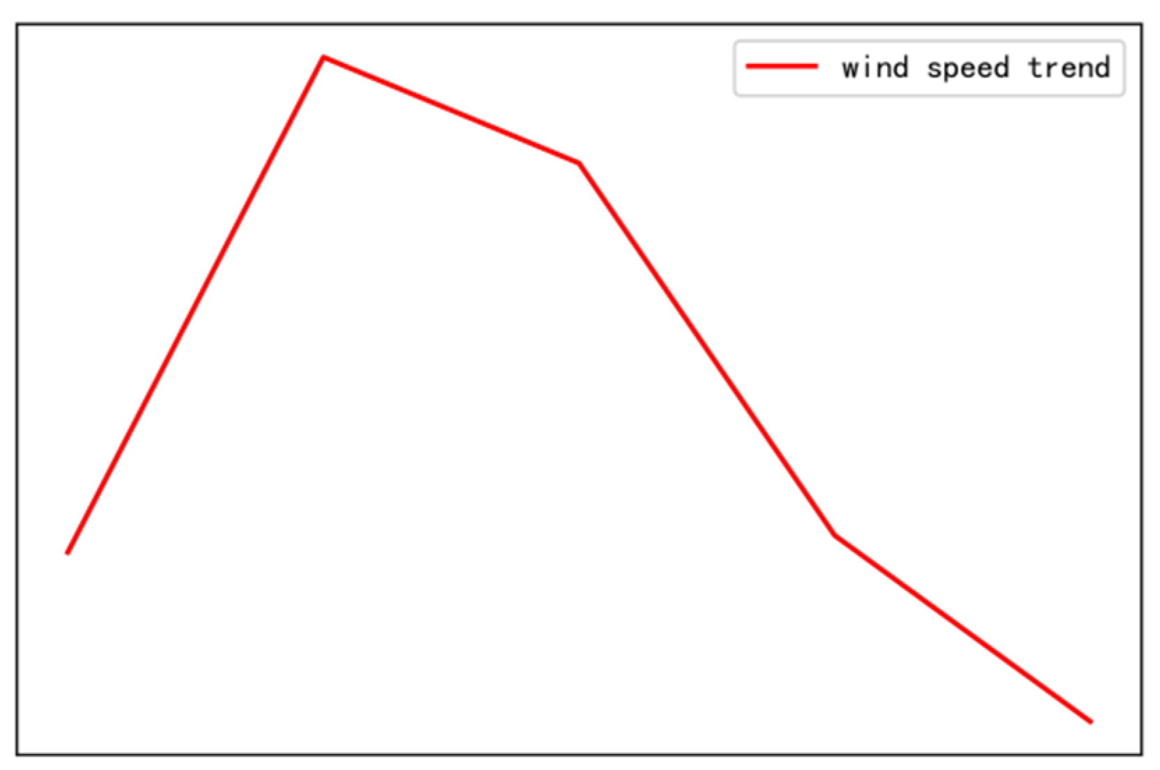
In order to more intuitively understand the collaborative filtering process and the results of wind speed patterns, this paper uses an example to illustrate. For the wind speed pattern Z to be matched, the pattern length is temporarily selected to be 5. Then, Z can be drawn as the curve in Figure 4.
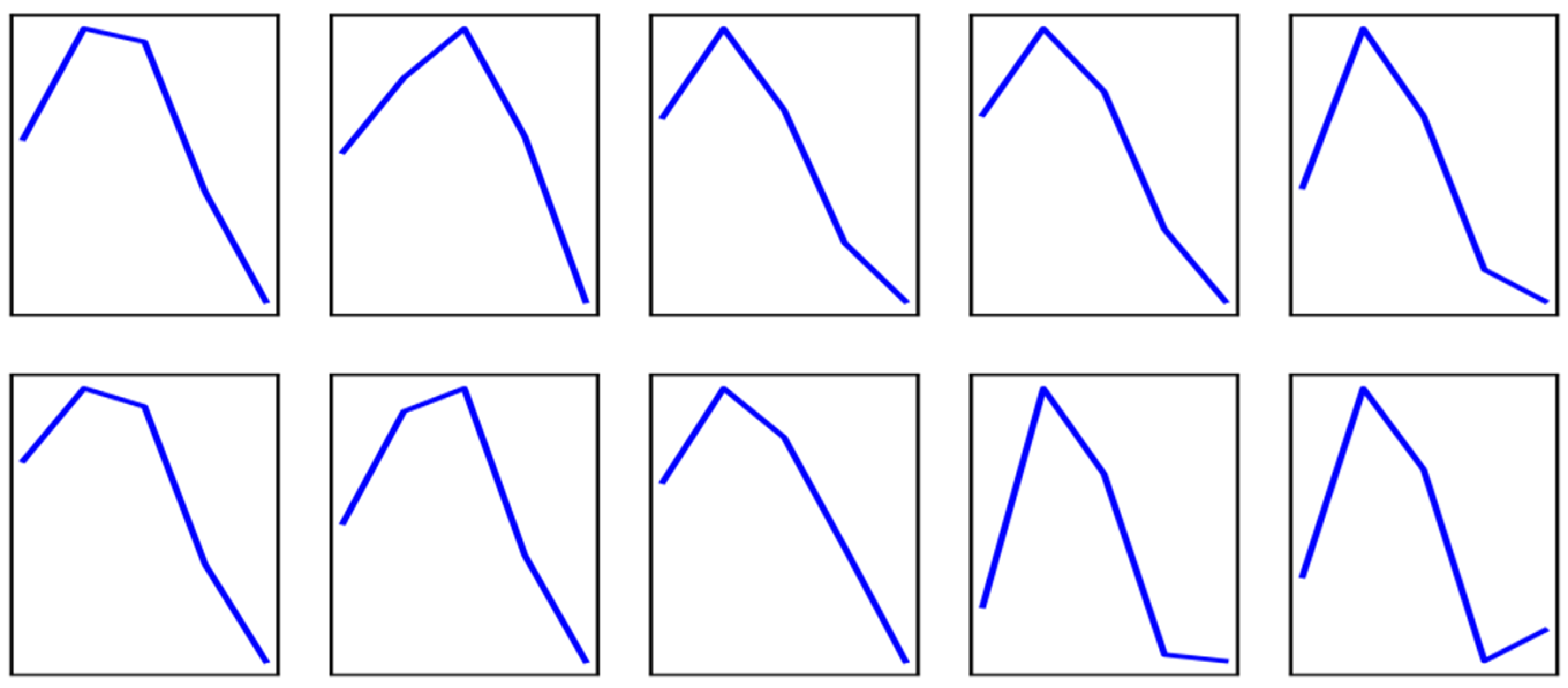
Then, by calculating the similarity between wind speed patterns, the top 10 similar wind speed patterns are screened out. The result of this step is implemented using a k-d tree to achieve the purpose of collaborative filtering of wind speed patterns. Likewise, plot them on the axes, as shown in Figure 5. It can be seen that the wind speed patterns from different time periods are similar to the wind speed variation trend of Z. We argue that they can be used to calculate the wind speed prediction for Z.
This article finds the corresponding true wind speed value yi in the set Y according to the index as part of the model input. However, if the only the similarity comparison is used, it may happen that two wind speed patterns have the same similarity as the pattern to be matched and cannot be distinguished. Therefore, in order to more accurately represent the difference and connection between wind speed patterns, this paper chooses to take distance into account, and further processes yi and distance to generate a new set of patterns. This will be illustrated in the algorithm of the collaborative filtering based wind speed prediction method, as shown in Algorithm 1.
| Algorithm 1 Wind speed prediction method based on collaborative filtering |
| Input: Wind power dataset; Output: Mean square error and root mean square error. 1. Load wind speed data and divide training set and test set for each set of wind speed series. 2. Perform pattern mining, preprocessing of the training set and test set, dividing wind speed data into two sets, X and Y. 3. Perform pattern matching, using the k-d tree to filter out the top-k patterns with the highest similarity, return the index and distance, and splice yi and distance together to generate a new pattern, set M. 4. Perform model training. Input the set M into the model, and train the model by continuously reducing the value of the loss function until convergence occurs. 5. Perform the wind speed forecast. Send the test set to the model to predict and evaluate the effect of the model with mean square error and root mean square error. |
3.4. Wind Speed Prediction Model Structure
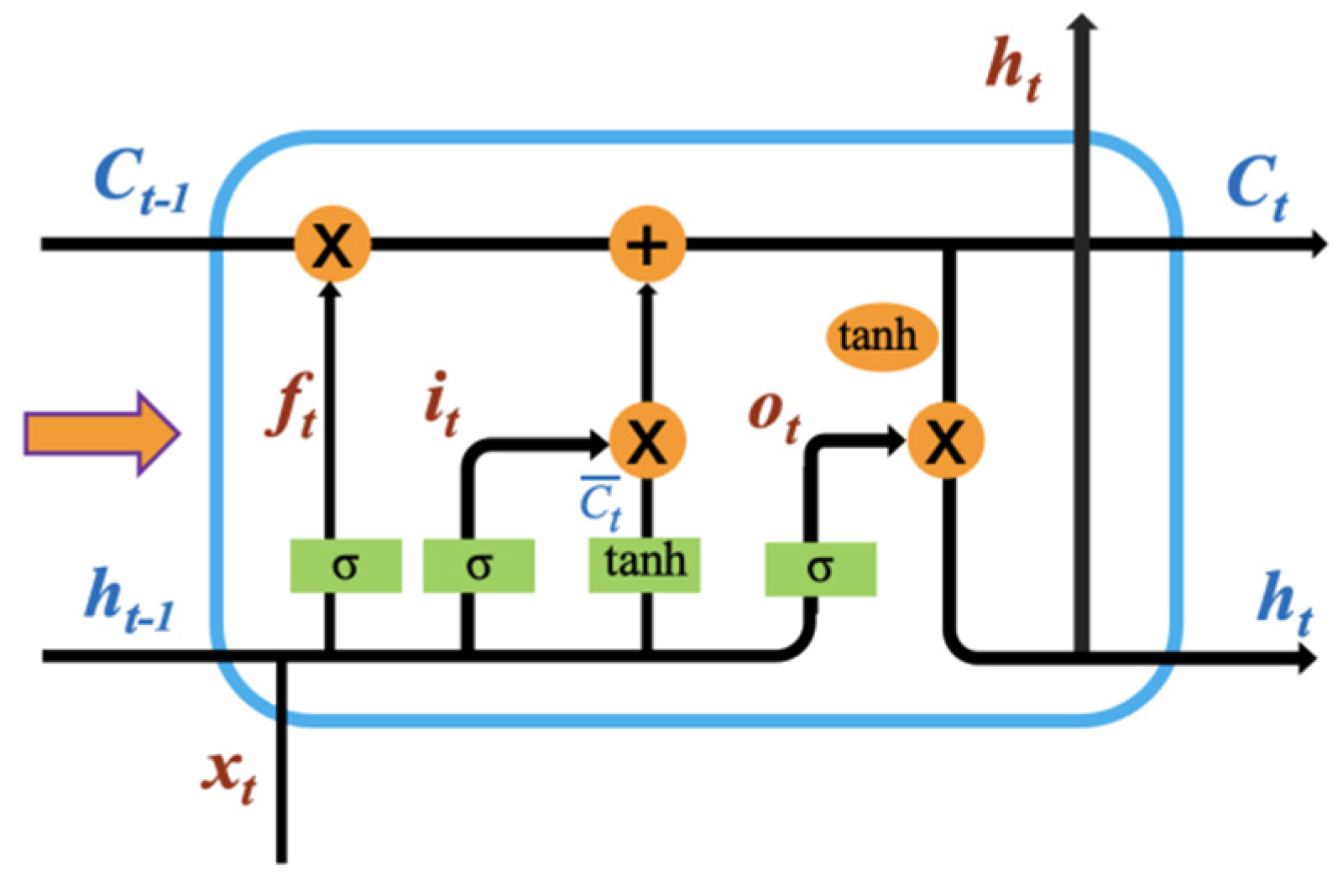
For the wind speed data obtained by collaborative filtering, this paper chooses the LSTM neural network as the main body of the training and prediction model. The unit structure of the LSTM network is shown in Figure 6.
Where, xt represents the input at time t; ht and ht−1 represent the output at time t and time t − 1, respectively; Ct and Ct−1 represent the cell state at time t and time t − 1, respectively. Ct represents the update value of the cell state at time t; ft, it and ot are the thresholds of the forget gate, the input gate and the output gate, respectively; tanh is the activation function. There are four small green frames in the middle cell, each of which represents a feedforward network layer. The σ parameter represents that the activation function of this layer is sigmoid, and the tanh parameter represents that the activation function of this layer is tanh.
The LSTM network is specially designed to solve the problem of long-term and short-term dependence caused by too long data in the general RNN, which enhances the long-term learning ability. The weight of the LSTM network is variable, which can better retain features while avoiding the problem of gradient disappearance or explosion. The hidden layer of the original RNN has only one state, so it is very sensitive to short-term input information. The hidden layer of LSTM has one more state than RNN, called the cell state. The unit state is parallel to the time axis, and the valid information at each moment is retained in the calculation process of the entire network, which can save the long-term state.
LSTM primarily functions through the gate structure, mainly including the forgetting gate, input gate, and output gate. The gate is a selective way of letting information through, and is composed of a sigmoid neural network and matrix point-by-point multiplication. The output of the gate is a vector of real numbers between 0 and 1. When the output is 0, no information is allowed to pass through; when the output is 1, any information can pass through. The following formula [40] describes the process of information transfer in detail.
The forget gate, which determines how much of the unit state at the previous moment is retained in the current moment. The calculation formula is defined as:
where and represent the weight and bias of the forget gate.
The input gate, which determines how much of the input of the network at the current moment and the output of the previous moment is saved to the unit state. This process can be formulated as:
where and represent the weight and bias of the input gate; and represent the weight and bias of the cell state.
Then, the input gate is merged with the output of the forget gate to update the cell state, as Formula (7). The cell state is not affected by weight parameters, which is the key to LSTM’s ability to effectively alleviate gradient disappearance.
The output gate determines how much of the unit state is output to the current output value of the LSTM, and the output value at the last moment is the predicted value of the model. The formula is represented by:
where and represent the weight and bias of the output gate.
The gate structure of the LSTM network uses the same calculation method to control the flow of information uniformly, and uses different weights and biases to update the three gating units independently when the error is back-propagated.
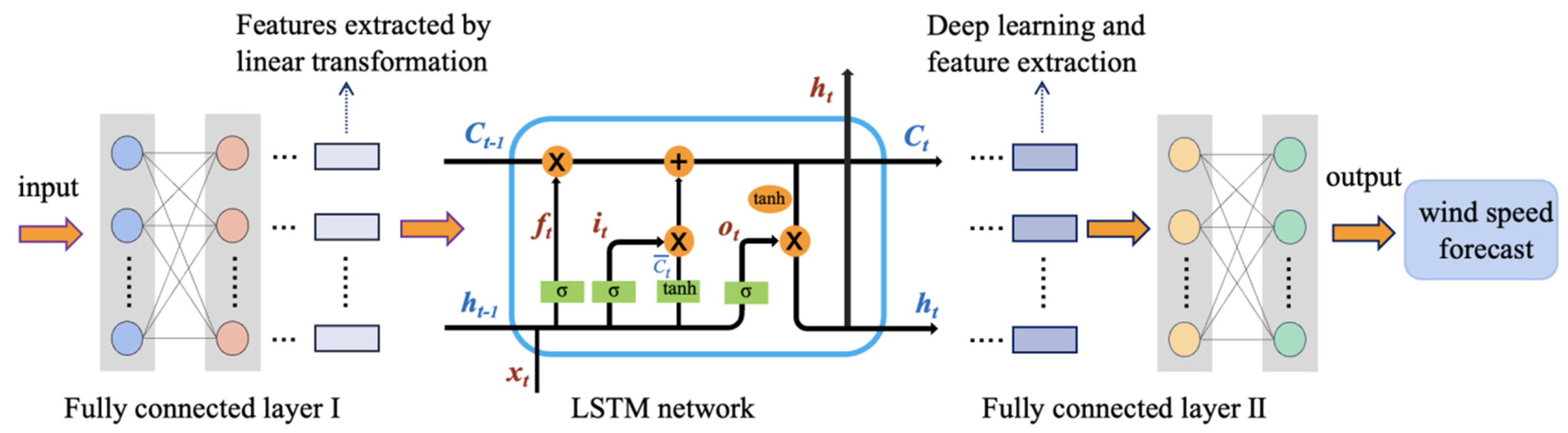
After wind speed preprocessing and collaborative filtering, a similar pattern set of wind speed patterns of the wind turbine to be predicted is screened out, and further processed as the input of the model. Due to the superiority of the LSTM network learning features, this paper chooses it as the main structure of the wind speed prediction model. The input size of the model in this paper is 2. The hidden layer has 2 layers, each with 40 neurons. Furthermore, to prevent non-linearity from destroying too much information, we also use fully connected layers. The overall model structure is shown in Figure 7.
First, after receiving the dataset M, processed based on the collaborative filtering algorithm, the input data is linearly transformed through the first fully connected layer to initially extract features. Then, the effective information of the data is learned by the LSTM network in a deeper level, and the information is controlled by the forgetting gate, the input gate, and the output gate, in turn. After the LSTM neural network is processed, the complex functional relationship of the extracted features is fitted through the second fully connected layer and mapped to the last network layer. Finally, the output layer outputs the result for wind speed prediction.
4. Experiments
4.1. Datasets and Evaluation Metrics
This paper uses data from the National Renewable Energy Laboratory (NREL) for the full year of 2010. The dataset includes 1380 wind turbines operating every 10 min, and each wind turbine includes approximately 105,121 records. The dataset includes eleven data, such as wind direction, wind speed, and wind power. During the experiment, 70% of the dataset is used as the training set, and the other 30% is used as the test set. The research goal of this paper is to predict the wind speed of a single wind turbine.
The software environment implemented by the model in this paper is python3.6, which is based on the machine learning framework Pytorch. In the training process, the batch size is 1000, the training process is set to 200 rounds of dataset iterations, the initial learning rate is 0.001, the dropout is set to 0.05, the Adam optimizer is used to optimize the training of the network, and all the results of the experiment are the average of multiple experiments.
We use mean squared error (MSE) and root mean squared error (RMSE) to evaluate the performance of the predictive models. The calculation process of MSE and RMSE is shown in Formulas (10) and (11), respectively.
where, yi represents the actual value of the wind speed, yipred represents the predicted value of the wind speed, and n represents the length of the wind speed sequence.
4.2. Experimental Results and Analysis
In order to achieve the best effect of the proposed method, the optimal pattern length is first selected through experiments. Taking the wind speed prediction of a single wind turbine as an example, based on extensive experiments done by the author during graduate school, the pattern lengths of the experiment are set to 3, 5, 7, 9, 11, 13, and 15, respectively, and 20 min is used as the forecast window. The experimental results are shown in Table 1.
As can be seen from the Table 1, the choice of pattern length will affect the prediction result, and if it is too large or too small, it will cause unsatisfactory effects. When the pattern length is 9, the value of MSE is the smallest. Therefore, the optimal pattern length in this experiment is 9; subsequent experiments will also use pattern sets of length 9.
In practice, when constructing a k-d tree with the wind speed pattern dataset, different distance metric algorithms can be selected when implementing the collaborative filtering algorithm, and the choice of the k-d tree metric algorithm will affect the return value and search efficiency. In order to perform pattern matching more efficiently, this paper conducts experiments on three metric algorithms of Euclidean distance, Manhattan distance, and Chebyshev distance, and chooses the optimal one. The experimental results are shown in Table 2.
From the MSE and RMSE indicators in the above table, the prediction effect of Euclidean distance is the best. In terms of the time predicted by the model, the Manhattan distance is more advantageous. This paper argues that it is acceptable to trade a slight time consumption for some degree of error reduction.
In this paper, ablation experiments are used to evaluate the contribution of the virtual edge expansion graph and the collaborative filtering algorithm to wind speed prediction.
Ablation Experiment 1: Evaluating the contribution of virtual edge expansion graphs to wind speed prediction. Using virtual edges to expand the graph, connect wind turbines in different regions to ensure that there is enough information to learn when extracting the spatiotemporal correlation of wind speed series. In fact, this is also the expansion and enhancement of the dataset of wind speed prediction. In order to verify that the application of a virtual edge expansion graph helps to improve the accuracy of wind speed prediction, the experiment randomly selects 50 wind turbines from a certain area in NERL 2010, connects virtual edges, and expands the size of the graph. Compared with the wind speed prediction using only the data from the wind turbine to be predicted, the experimental results are shown in Table 3.
From the experimental results in the Table 3, it can be seen that the prediction error of expanding the graph with virtual edges is 11.03% lower than that of expanding the graph without virtual edges. The 50 wind turbines used for the virtual edge connection expansion graph are randomly selected from the dataset, which ensures the reliability of the experimental results. Therefore, the experiment proves that in the problem of wind speed prediction, the application of a virtual edge expansion graph to expand and enhance the wind speed dataset is helpful to improve the accuracy of wind speed prediction.
This paper uses the collaborative filtering algorithm for wind speed prediction, which is also an enhancement to the dataset, making the characteristics of the wind speed series more prominent in order to verify that applying the data of multiple wind turbines helps to improve the accuracy of wind speed prediction. In the experiment, 50 wind turbines were randomly selected from NERL in 2010, and compared with only one wind turbine for wind speed prediction; the experimental results are shown in Table 3.
Ablation Experiment 2: Evaluating the contribution of collaborative filtering algorithms to wind speed prediction. The preprocessing method of wind speed is not changed, and the set of mode X and true wind speed value Y are still retained. However the, k-d tree is no longer used to implement the collaborative filtering algorithm for wind speed pattern matching. That is to say, the preprocessed wind speed data is directly fed into the model to train the model and predict the wind speed. The experimental results are shown in Table 4.
As can be seen from the above table, the performance improvement of the model using the collaborative filtering algorithm is obvious, and the wind speed prediction error is reduced by 26.89%, compared with the wind speed prediction error without the collaborative filtering algorithm. Although the prediction time has increased by 18.62% at the same time, the authors believe that such time consumption is worthwhile.
Based on the above experiments, in order to verify the effectiveness of the method proposed in this paper, it is compared with some popular machine learning methods in the NREL dataset, including KNN, SVR, Bayesian regression, and XGBoost models; the following is a brief introduction. During the experiment, models such as KNN do the same preprocessing and adjust the parameters to optimal values, but do not use collaborative filtering algorithm processing.
- KNN [41]: It is a commonly used data mining algorithm. The basic principle is to find k points similar to the point to be predicted through a distance metric relationship, and then perform regression prediction based on these k points.
- SVR [42]: It is an important branch of support vector machine leraning, based on finding a hyperplane such that the distance from all data to this hyperplane is minimized; it is often used in regression problems.
- Bayesian regression [43]: The basic idea is to treat the dataset and parameters as a known distribution, predicting the posterior probability distribution based on the known prior probability distribution of historical observations.
- XGBoost [44]: It is essentially an iterative decision tree algorithm, which is improved based on the gradient boosting tree (GBDT), which effectively avoids overfitting and improves the speed and accuracy of the model.
The experiment uses the data of 1380 wind turbines in the entire year of NERL 2010. The final experimental results are shown in Table 5.
As can be seen from Table 5, compared with KNN, SVR, Bayesian regression, and XGBoost models, the MSE of the proposed method is reduced by 16.40%, 11.78%, 9.57% and 18.36%, respectively. The time for model learning and prediction is also within an acceptable range, which proves the effectiveness and stability of the method proposed in this paper.
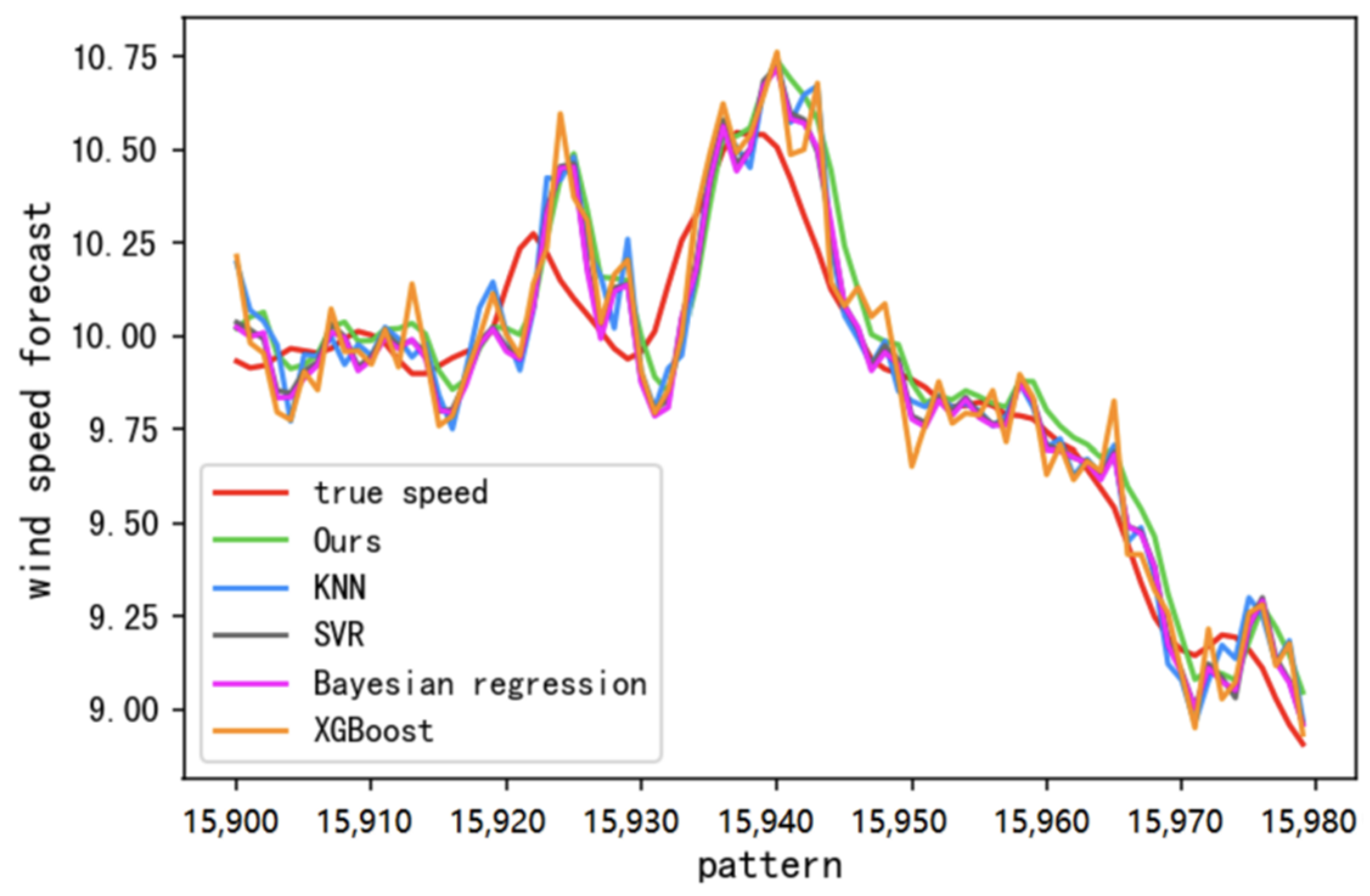
In order to intuitively compare the performance of the method proposed in this paper with these typical machine learning models, we draw the trend curves of their predicted wind speed and actual wind speed, as shown in Figure 8.
We randomly selected the results of 80 patterns in the set, which can be used as a timeline because the patterns are divided in chronological order. It can be seen that the method proposed in this paper performs better than other models and can well fit the actual change of wind speed.
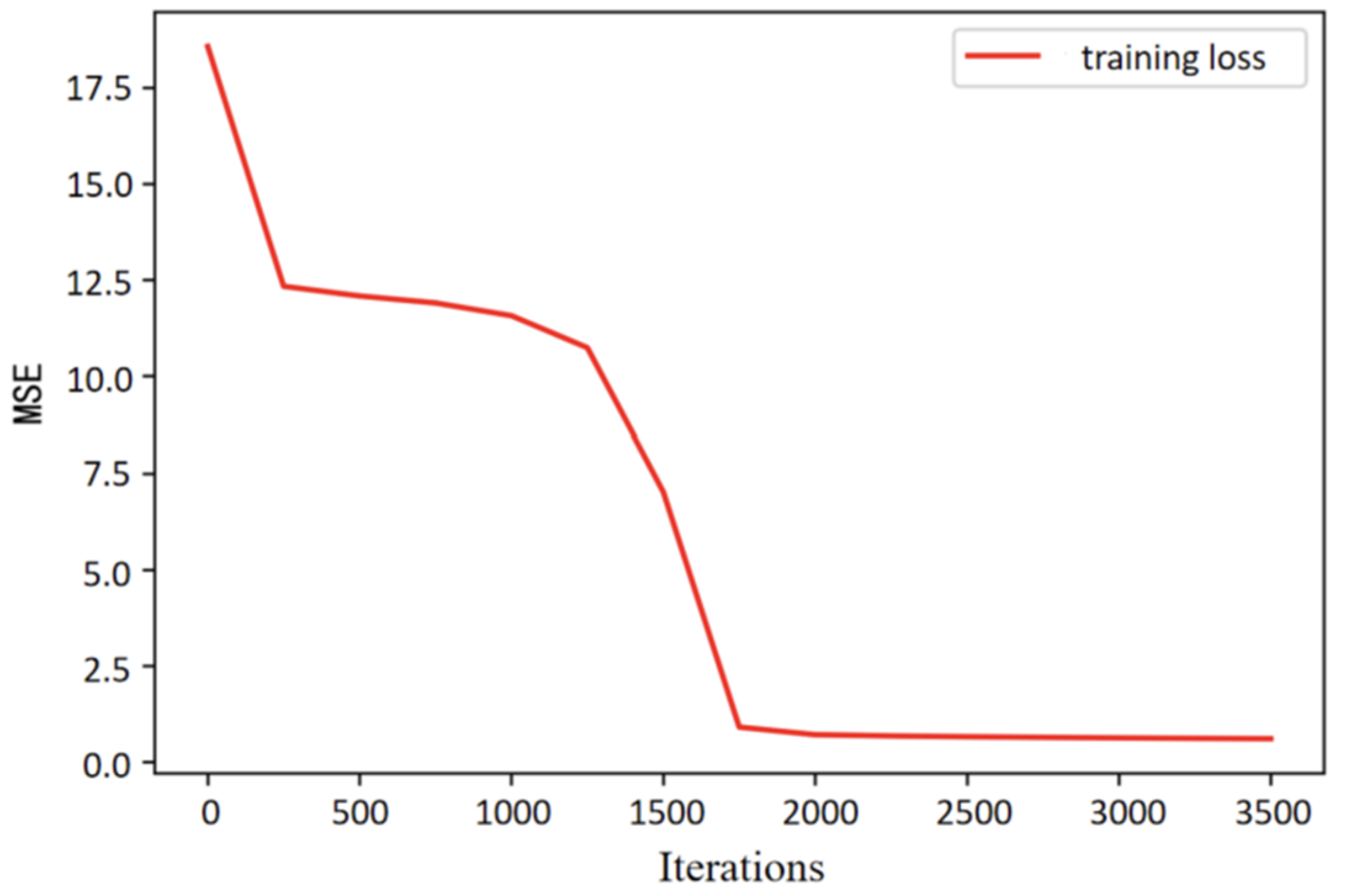
In addition, in order to observe the convergence performance of the model, we also plot the decrease in the loss value of the proposed method during model training. The x-axis represents the number of iterations, and the y-axis is the MSE value between the actual wind speed value and the predicted wind speed value, as shown in the Figure 9.
It can be seen that the convergence speed of the model is very considerable, the number of iterations tends to be stable at about 1700 times, and the loss value is relatively small, which further shows the superiority of the method proposed in this paper in extracting features and predicting wind speed.
5. Conclusions
In order to solve the problem that the data source is limited to a fixed area and the spatiotemporal correlation of wind speed sequences is not sufficiently mined in wind speed prediction, this paper proposes a wind speed prediction method based on a virtual edge expansion graph and a collaborative filtering algorithm from three aspects: dataset source, wind speed data processing, and modeling mechanism. The virtual edge expansion graph expands the wind speed dataset, making the number of wind speed sequences mineable enough. The collaborative filtering algorithm considers the spatiotemporal correlation of the wind speed sequence, preprocesses the wind speed sequence, and uses a k-d tree for wind speed pattern matching. Finally, the set of similar wind speed patterns of the wind turbine to be predicted input into the long short-term memory (LSTM) based model for training and prediction. The experimental results show that the virtual edge expansion graph and the collaborative filtering algorithm can improve the prediction effect of the model, and the method proposed in this paper outperforms other comparison models for different indicators.
Author Contributions
Investigation, D.H.; methodology, Z.L.; project administration, J.G.; resources, X.Y.; supervision, W.X.; writing—original draft, K.Z.; writing—review and editing, X.L. All authors have read and agreed to the published version of the manuscript.
Funding
This research was funded by National Natural Science Foundation of China (Grant No. 61976155) and the Tianjin Technical Export Project (No. 20YDTPJC01570).
Institutional Review Board Statement
Not applicable.
Informed Consent Statement
Not applicable.
Data Availability Statement
Publicly available datasets were analyzed in this study. This data can be found here: https://www.nrel.gov (accessed on 8 December 2021).
Conflicts of Interest
The authors declare no conflict of interest.
References
- Jørgensen, K.L.; Shaker, H.R. Wind Power Forecasting Using Machine Learning: State of the Art, Trends and Challenges. In Proceedings of the 2020 IEEE 8th International Conference on Smart Energy Grid Engineering (SEGE), Oshawa, ON, Canada, 12–14 August 2020; IEEE: Piscataway, NJ, USA, 2020; pp. 44–50. [Google Scholar] [CrossRef]
- Liu, H.; Yang, R.; Wang, T.; Zhang, L. A hybrid neural network model for short-term wind speed forecasting based on decomposition, multi-learner ensemble, and adaptive multiple error corrections. Renew. Energy 2021, 165, 573–594. [Google Scholar] [CrossRef]
- Chen, X.; Lai, C.S.; Ng WW, Y.; Pan, K.; Lai, L.L.; Zhong, C. A stochastic sensitivity-based multi-objective optimization method for short-term wind speed interval prediction. Int. J. Mach. Learn. Cybern. 2021, 12, 2579–2590. [Google Scholar] [CrossRef]
- Zhao, X.; Liu, J.; Yu, D.; Chang, J. One-day-ahead probabilistic wind speed forecast based on optimized numerical weather prediction data. Energy Convers. Manag. 2018, 164, 560–569. [Google Scholar] [CrossRef]
- Moreno, S.R.; da Silva, R.G.; Mariani, V.C.; Santos, C.L.D. Multi-step wind speed forecasting based on hybrid multi-stage decomposition model and long short-term memory neural network. Energy Convers. Manag. 2020, 213, 112869. [Google Scholar] [CrossRef]
- Senthil, K.P. Improved prediction of wind speed using machine learning. EAI Endorsed Trans. Energy Web 2019, 6, e2. [Google Scholar] [CrossRef] [Green Version]
- Zhao, J.; Guo, Z.H.; Su, Z.Y.; Zhao, Z.Y.; Xiao, X.; Liu, F. An improved multi-step forecasting model based on WRF ensembles and creative fuzzy systems for wind speed. Appl. Energy 2016, 162, 808–826. [Google Scholar] [CrossRef]
- Yan, J.; Li, K.; Bai, E.; Zhao, X.; Xue, Y.; Foley, A.M. Analytical iterative multistep interval forecasts of wind generation based on TLGP. IEEE Trans. Sustain. Energy 2018, 10, 625–636. [Google Scholar] [CrossRef] [Green Version]
- Erdem, E.; Shi, J. ARMA based approaches for forecasting the tuple of wind speed and direction. Appl. Energy 2011, 88, 1405–1414. [Google Scholar] [CrossRef]
- Singh, S.N.; Mohapatra, A. Repeated wavelet transform based ARIMA model for very short-term wind speed forecasting. Renew. Energy 2019, 136, 758–768. [Google Scholar] [CrossRef]
- Aly HH, H. An intelligent hybrid model of neuro Wavelet, time series and Recurrent Kalman Filter for wind speed forecasting. Sustain. Energy Technol. Assess. 2020, 41, 100802. [Google Scholar] [CrossRef]
- Li, W.; Jia, X.; Li, X.; Wang, Y.; Lee, J. A Markov model for short term wind speed prediction by integrating the wind acceleration information. Renew. Energy 2021, 164, 242–253. [Google Scholar] [CrossRef]
- Chen, K.; Yu, J. Short-term wind speed prediction using an unscented Kalman filter based state-space support vector regression approach. Appl. Energy 2014, 113, 690–705. [Google Scholar] [CrossRef]
- Wen, Y.; Song, M.; Wang, J. A combined AR-kNN model for short-term wind speed forecasting. In Proceedings of the 2016 IEEE 55th Conference on Decision and Control (CDC), Las Vegas, NV, USA, 12–14 December 2016; IEEE: Piscataway, NJ, USA, 2016; pp. 6342–6346. [Google Scholar] [CrossRef]
- Samadianfard, S.; Hashemi, S.; Kargar, K.; Izadyar, M.; Mostafaeipour, A.; Mosavi, A.; Shamshirband, S. Wind speed prediction using a hybrid model of the multi-layer perceptron and whale optimization algorithm. Energy Rep. 2020, 6, 1147–1159. [Google Scholar] [CrossRef]
- Jin, D.; You, X.; Li, W.; He, D.; Cui, P.; Fogelman-Soulié, F.; Chakraborty, T. Incorporating network embedding into markov random field for better community detection. In Proceedings of the AAAI Conference on Artificial Intelligence, Honolulu, HI, USA, 27 January–1 February 2019; Volume 33, pp. 160–167. [Google Scholar] [CrossRef]
- Duan, J.; Zuo, H.; Bai, Y.; Chang, M.; Chen, B. Short-term wind speed forecasting using recurrent neural networks with error correction. Energy 2020, 217, 119397. [Google Scholar] [CrossRef]
- Ehsan, M.A.; Shahirinia, A.; Zhang, N.; Oladunni, T. Wind Speed Prediction and Visualization Using Long Short-Term Memory Networks (LSTM). In Proceedings of the 2020 10th International Conference on Information Science and Technology (ICIST), Plymouth, UK, 9–15 September 2020; IEEE: Piscataway, NJ, USA, 2020; pp. 234–240. [Google Scholar] [CrossRef]
- Trebing, K.; Mehrkanoon, S. Wind speed prediction using multidimensional convolutional neural networks. In Proceedings of the 2020 IEEE Symposium Series on Computational Intelligence (SSCI), Canberra, Australia, 1–4 December 2020; IEEE: Piscataway, NJ, USA, 2020; pp. 713–720. [Google Scholar] [CrossRef]
- Yang, F.; Zhang, H.; Tao, S. Hybrid deep graph convolutional networks. Int. J. Mach. Learn. Cybern. 2022, 11, 1–17. [Google Scholar] [CrossRef]
- Ding, G.; Qin, L. Study on the prediction of stock price based on the associated network model of LSTM. Int. J. Mach. Learn. Cybern. 2020, 11, 1307–1317. [Google Scholar] [CrossRef] [Green Version]
- Du, B.; Peng, H.; Wang, S.; Bhuiyan MZ, A.; Wang, L.; Gong, Q.; Li, J. Deep irregular convolutional residual LSTM for urban traffic passenger flows prediction. IEEE Trans. Intell. Transp. Syst. 2019, 21, 972–985. [Google Scholar] [CrossRef]
- Zhang, Y.; Lu, M.; Li, H. Urban traffic flow forecast based on FastGCRNN. J. Adv. Transp. 2020, 2020, 8859538. [Google Scholar] [CrossRef]
- Peng, H.; Wang, H.; Du, B.; Bhuiyan, M.Z.A.; Ma, H.; Liu, J.; Yu, P.S. Spatial temporal incidence dynamic graph neural networks for traffic flow forecasting. Inf. Sci. 2020, 521, 277–290. [Google Scholar] [CrossRef]
- Cheng, L.; Zang, H.; Xu, Y.; Wei, Z.; Sun, G. Augmented Convolutional Network for Wind Power Prediction: A New Recurrent Architecture Design With Spatial-Temporal Image Inputs. IEEE Trans. Ind. Inform. 2021, 17, 6981–6993. [Google Scholar] [CrossRef]
- Jiajun, H.; Chuanjin, Y.; Yongle, L.; Huoyue, X. Ultra-short term wind prediction with wavelet transform, deep belief network and ensemble learning. Energy Convers. Manag. 2020, 205, 112418. [Google Scholar] [CrossRef]
- Abedinia, O.; Lotfi, M.; Sobhani, B.; Shafie-khah, M.; Catalao, J.P.S. Improved EMD-based complex prediction model for wind power forecasting. IEEE Trans. Sustain. Energy 2020, 11, 2790–2802. [Google Scholar] [CrossRef]
- Hu, H.; Wang, L.; Tao, R. Wind speed forecasting based on variational mode decomposition and improved echo state network. Renew. Energy 2021, 164, 729–751. [Google Scholar] [CrossRef]
- Chen, Y.; Dong, Z.; Wang, Y.; Su, J.; Han, Z.; Zhou, D.; Bao, Y. Short-term wind speed predicting framework based on EEMD-GA-LSTM method under large scaled wind history. Energy Convers. Manag. 2021, 227, 113559. [Google Scholar] [CrossRef]
- Chao, G.; Luo, Y.; Ding, W. Recent advances in supervised dimension reduction: A survey. Mach. Learn. Knowl. Extr. 2019, 1, 20. [Google Scholar] [CrossRef] [Green Version]
- Saxena, A.; Prasad, M.; Gupta, A.; Bharill, N.; Prakash, O.P.; Tiwari, A.; Tiwari, M.E.; Ding, W.; Lin, C.T. A review of clustering techniques and developments. Neurocomputing 2017, 267, 664–681. [Google Scholar] [CrossRef] [Green Version]
- Zhu, Q.; Chen, J.; Shi, D.; Zhu, L.; Bai, X.; Duan, X.; Liu, Y. Learning temporal and spatial correlations jointly: A unified framework for wind speed prediction. IEEE Trans. Sustain. Energy 2019, 11, 509–523. [Google Scholar] [CrossRef]
- Tao, H.; Lu, X. On comparing six optimization algorithms for network-based wind speed forecasting. In Proceedings of the 2018 37th Chinese Control Conference (CCC), Wuhan, China, 25–27 July 2018; IEEE: Piscataway, NJ, USA, 2018; pp. 8843–8850. [Google Scholar] [CrossRef]
- Subramaniam Nachimuthu, D.; Banerjee, A.; Karuppaiah, J. Multi-step wind speed and wind power forecasting using variational momentum factor and deep learning based intelligent neural network models. Concurr. Comput. Pract. Exp. 2022, 34, e6772. [Google Scholar] [CrossRef]
- Zhang, Z.; Ye, L.; Qin, H.; Liu, Y.; Wang, C.; Yu, X.; Li, J. Wind speed prediction method using shared weight long short-term memory network and Gaussian process regression. Appl. Energy 2019, 247, 270–284. [Google Scholar] [CrossRef]
- Ekstrand, M.D.; Riedl, J.T.; Konstan, J.A. Collaborative Filtering Recommender Systems. In Foundations and Trends in Human-Computer Interaction; Now Publishers Inc.: Boston, MA, USA, 2011. [Google Scholar] [CrossRef]
- Ding, L.; Han, B.; Wang, S.; Li, X.; Song, B. User-centered recommendation using US-ELM based on dynamic graph model in E-commerce. Int. J. Mach. Learn. Cybern. 2019, 10, 693–703. [Google Scholar] [CrossRef]
- Das, J.; Majumder, S.; Gupta, P.; Mali, K. Collaborative recommendations using hierarchical clustering based on Kd trees and quadtrees. Int. J. Uncertain. Fuzziness Knowl.-Based Syst. 2019, 27, 637–668. [Google Scholar] [CrossRef]
- Chen, F.; Wang, Y.C.; Wang, B.; Kuo, C.C.J. Graph representation learning: A survey. APSIPA Trans. Signal Inf. Process. 2020, 9, E15. [Google Scholar] [CrossRef]
- Graves, A. Supervised Sequence Labelling with Recurrent Neural Networks; Studies in Computational Intelligence; Springer: Cham, Switzerland, 2012. [Google Scholar] [CrossRef] [Green Version]
- Martínez, F.; Frías, M.P.; Pérez, M.D.; Rivera, A.J. A methodology for applying k-nearest neighbor to time series forecasting. Artif. Intell. Rev. 2019, 52, 2019–2037. [Google Scholar] [CrossRef]
- Santamaría-Bonfil, G.; Reyes-Ballesteros, A.; Gershenson, C. Wind speed forecasting for wind farms: A method based on support vector regression. Renew. Energy 2016, 85, 790–809. [Google Scholar] [CrossRef]
- Wang, Y.; Wang, H.; Srinivasan, D.; Hu, Q. Robust functional regression for wind speed forecasting based on Sparse Bayesian learning. Renew. Energy 2019, 132, 43–60. [Google Scholar] [CrossRef]
- Phan, Q.T.; Wu, Y.K.; Phan, Q.D. A Hybrid Wind Power Forecasting Model with XGBoost, Data Preprocessing Considering Different NWPs. Appl. Sci. 2021, 11, 1100. [Google Scholar] [CrossRef]
Figure 1.
A wind farm graph.

Figure 2.
Actual edge connection graph.

Figure 3.
Virtual edge expansion graph.

Figure 4.
Wind speed pattern curve.

Figure 5.
Results of collaborative filtering for wind speed patterns.

Figure 6.
LSTM network unit structure.

Figure 7.
Overall model structure.

Figure 8.
Curves of the Wind speed trend.

Figure 9.
Loss drop plot for the proposed model.


Table 1.
Comparison of wind speed errors using different pattern lengths.
| Pattern Length | 3 | 5 | 7 | 9 | 11 | 13 | 15 |
|---|---|---|---|---|---|---|---|
| MSE | 0.3885 | 0.3446 | 0.3165 | 0.3019 | 0.3205 | 0.3442 | 0.3955 |
| RMSE | 0.6233 | 0.5870 | 0.5625 | 0.5494 | 0.5661 | 0.5867 | 0.6288 |
Table 2.
Experimental results of k-d tree using different metric algorithms.
| Algorithms | Euclidean | Manhattan | Chebyshev |
|---|---|---|---|
| MSE | 0.3019 | 0.3217 | 0.3150 |
| RMSE | 0.5494 | 0.5671 | 0.5612 |
| Time (s) | 949.56 | 880.21 | 2200.72 |
Table 3.
Ablation Experiment 1: Whether to expand the graph with virtual edges.
| Whether to Expand the Graph with Virtual Edges | Yes | No |
|---|---|---|
| MSE | 0.2743 | 0.3083 |
| RMSE | 0.5237 | 0.5552 |
| Time (s) | 892.94 | 677.64 |
Table 4.
Ablation Experiment 2: Whether to use collaborative filtering algorithm.
| Whether to Use Collaborative Filtering | Yes | No |
|---|---|---|
| MSE | 0.2743 | 0.3752 |
| RMSE | 0.5237 | 0.6125 |
| Time (s) | 892.94 | 726.64 |
Table 5.
Experimental results of comparative experiments.
| Models | Ours | KNN | SVR | Bayesian Regression | XGBoost |
|---|---|---|---|---|---|
| MSE | 0.2636 | 0.3153 | 0.2988 | 0.2915 | 0.3229 |
| RMSE | 0.5134 | 0.5615 | 0.5466 | 0.5399 | 0.5682 |
| Time (s) | 3168.11 | 1040.26 | 1447.17 | 1377.97 | 1889.08 |
Publisher’s Note: MDPI stays neutral with regard to jurisdictional claims in published maps and institutional affiliations. |
© 2022 by the authors. Licensee MDPI, Basel, Switzerland. This article is an open access article distributed under the terms and conditions of the Creative Commons Attribution (CC BY) license (https://creativecommons.org/licenses/by/4.0/).
Share and Cite
MDPI and ACS Style
Ying, X.; Zhao, K.; Liu, Z.; Gao, J.; He, D.; Li, X.; Xiong, W. Wind Speed Prediction via Collaborative Filtering on Virtual Edge Expanding Graphs. Mathematics 2022, 10, 1943. https://0-doi-org.brum.beds.ac.uk/10.3390/math10111943
AMA Style
Ying X, Zhao K, Liu Z, Gao J, He D, Li X, Xiong W. Wind Speed Prediction via Collaborative Filtering on Virtual Edge Expanding Graphs. Mathematics. 2022; 10(11):1943. https://0-doi-org.brum.beds.ac.uk/10.3390/math10111943
Chicago/Turabian StyleYing, Xiang, Keke Zhao, Zhiqiang Liu, Jie Gao, Dongxiao He, Xuewei Li, and Wei Xiong. 2022. "Wind Speed Prediction via Collaborative Filtering on Virtual Edge Expanding Graphs" Mathematics 10, no. 11: 1943. https://0-doi-org.brum.beds.ac.uk/10.3390/math10111943
Note that from the first issue of 2016, this journal uses article numbers instead of page numbers. See further details here.