A Novel Multi-Objective Hybrid Election Algorithm for Higher-Order Random Satisfiability in Discrete Hopfield Neural Network

Abstract

Hybridized algorithms are commonly employed to improve the performance of any existing method. However, an optimal learning algorithm composed of evolutionary and swarm intelligence can radically improve the quality of the final neuron states and has not received creative attention yet. Considering this issue, this paper presents a novel metaheuristics algorithm combined with several objectives—introduced as the Hybrid Election Algorithm (HEA)—with great results in solving optimization and combinatorial problems over a binary search space. The core and underpinning ideas of this proposed HEA are inspired by socio-political phenomena, consisting of creative and powerful mechanisms to achieve the optimal result. A non-systematic logical structure can find a better phenomenon in the study of logic programming. In this regard, a non-systematic structure known as Random k Satisfiability (RANkSAT) with higher-order is hosted here to overcome the interpretability and dissimilarity compared to a systematic, logical structure in a Discrete Hopfield Neural Network (DHNN). The novelty of this study is to introduce a new multi-objective Hybrid Election Algorithm that achieves the highest fitness value and can boost the storage capacity of DHNN along with a diversified logical structure embedded with RANkSAT representation. To attain such goals, the proposed algorithm tested four different types of algorithms, such as evolutionary types (Genetic Algorithm (GA)), swarm intelligence types (Artificial Bee Colony algorithm), population-based (traditional Election Algorithm (EA)) and the Exhaustive Search (ES) model. To check the performance of the proposed HEA model, several performance metrics, such as training–testing, energy, similarity analysis and statistical analysis, such as the Friedman test with convergence analysis, have been examined and analyzed. Based on the experimental and statistical results, the proposed HEA model outperformed all the mentioned four models in this research.

1. Introduction

The term Artificial Neural Network (ANN) refers to generalizations of mathematical models of the biological nervous system. Over the previous two decades, researchers have enhanced the potentiality of ANNs, which added a new dimension to the study of numerous scientific subjects. Dr Hopfield advanced the dynamics of ANN by proposing a method for integrating feedback loop mechanisms, named the Hopfield Neural Network (HNN) [1]. With a recursive structure and graded response, this HNN, one of the earliest types of neural networks, is akin to a dynamic system with two or more stable points of equilibrium [2]. This HNN has variety and is potentially useful for health [3], behavioral sciences [4], and energy [5]. However, the HNN not only always converges to an exact pattern, which results in sub-optimal solutions but also suffers highly from its storage capacity. In such a case, the introduction of logic programming can be a good counter. Following this research, we explore the connections as a single symbolic instruction and its nature into logical rule assemblies using HNN.

Satisfiability (SAT) representation is an important means of conveying logical rules with mathematical information in AI through ANNs. In this context, a general query arises—is the SAT necessary in a Discrete Hopfield Neural Network (DHNN)? To answer this, SAT is designed to be readily attached as a symbolic instruction to represent the output of DHNN. Abdullah invented the general concept of logic programming on DHNN by computing the synaptic weights [6]. Later, a study [7] introduced new light to the satisfiability study. This work proposed a higher-order Horn-Satisfiability (Horn-SAT) programming, which focused on embedding Horn-clauses in a Radial Basis Function Neural Network. Therefore, several researchers further extended the fundamentals of Horn-SAT by proposing different systematic k Satisfiability (k-SAT), such as 2SAT and 3SAT. The work by [8] transformed the constraint satisfaction problem into the 2SAT problem, which is more effective in achieving a different number of solutions. Then, the work by [9] introduced the systematic 3SAT logical expression with a well-known metaheuristics Genetic Algorithm (GA). This work explored previous works to direct the search into regions of better performance within the search space, thus, reducing the time and space complexity. Maximum k Satisfiability (MAXkSAT), inspired by an expanded version of Boolean SAT, began to gain favor in the ANN research field because it used false/negative output in comparison to other SAT presentations [10]. Following that, [11] developed a hybrid technique that uses an algorithm to optimize the 2SAT logical rule. This work has risen to a new type of SAT study known as Maximum 2 Satisfiability (MAX2SAT). For its nonredundant literals, the result of this MAX2SAT logical rule was also negative. The proposed approach could display MAX2SAT behavior optimally during the DHNN testing phase. However, there is no involvement of any process that can minimize the complexity of the MAX2SAT model in the training phase. Subsequently, these studies investigated only the systematic logical rule. The first attempt is to represent the symbolic output of the HNN in terms of the non-systematic logical rule made by [12]. This research showed that Random 2 Satisfiability (RAN2SAT) can be integrated into DHNN by minimizing a cost function that corresponds to the network inconsistencies. Nonetheless, this work restricted only k = 1, 2 in which no discussions were made on improvement strategy for k = 1, 2, 3 or Horn Satisfiability. Another different type of non-systematic logical rule was sketched by [13]. This study was a new variant of the 2 Satisfiability problems. This work revealed that Major 2 Satisfiability (MAJ2SAT) is able to provide a new perspective in representing some NP and probabilistic class problems. The non-systematic logic study was further extended by [14], proposing a new dimension in the non-systematic Random k Satisfiability (RANkSAT) study. This work showed the achievement of 100% accurate synaptic weights by a higher order of RANkSAT (k = 3, 2) combination leads to 100% global minima solutions. Though some researchers continue to focus on the usefulness of non-systematic logical rules in DHNN, the notion has yet to be fully explored.

The effectiveness of a learning phase is a significant issue in DHNN. Ref. [15] revealed the weakness of HNN as the number of neurons grows in terms of retrieval capacity. To address this issue, a metaheuristic method was used to determine the best neuron state that minimizes the cost function. Another significant work was proposed by [16], in which the Hybrid Genetic Algorithm (GA) was incorporated with the training phase of HNN. This hybrid model successfully obtained the best trade-off between solution quality and computational time. Another study conducted by [17] demonstrated the Artificial Immune System (AIS) in the training phase with the 3SAT logical rule. This investigation explained that AIS outperformed the Brute-Force algorithm in terms of the global minima ratio, hamming distance and computational time. Ref. [18] successfully integrated the usage of GA with HNN for solving combinatorial optimization problems. In their study, the HNN was applied to GA to minimize each other’s shortcomings. The combination of both methods reduces the possible local minima in solving various NP problems. Furthermore, [19] introduced propositional satisfiability via a hybrid metaheuristic named Hybrid Genetic Algorithm (HGA) in DHNN. This work explained that GA as a non-biased algorithm can converge to a global solution compared to conventional learning models. Finally, the authors [20] developed a hybrid HNN and integrated it with an Imperialist Competitive Algorithm (ICA). This proposed hybrid method successfully found an optimal solution in an acceptable computation time and managed to obtain a high-quality solution with minimum cost. However, these metaheuristics focused exclusively on systematic logical rules. Additionally, these metaheuristics lack a partition solution space for which a more efficient solution is required to identify alternative neuron states to minimize the cost function. Moreover, the mentioned metaheuristics have no specific balance with the extrapolation and exploitation strategy.

Recently, social and political behaviours have also inspired the development of numerous metaheuristic solvers. An election Algorithm (EA) is a form of an iterative social-political algorithm that operates on populations of solutions via the ‘election’ procedure. Ref. [21] addressed this Election Algorithm (EA) as a highly optimized metaheuristic for its powerful solution search space, drawing the attention of many optimization researchers. EA is a population-based iterative algorithm that works with solution groups. First, the population will be divided into several parties based on their shared beliefs and views, the best members of each party will be chosen as candidates, while the others will be voters who support the candidate. Since EA suffers from a fundamental challenge; it always becomes stuck at local optima due to the incapability of the operators. To overcome this issue, later, the author [22] proposed the Chaotic Election Algorithm (CEA), which accelerates the convergence of the existing EA by introducing a migration operator. However, these works also have no justification for several objectives to enhance the capacity of these metaheuristics.

Research recently indicated that non-systematic logical rules can provide a flexible structure and generate various interpretations that converge to global minimum solutions. Pioneering work by [23] created a bridge between logic programming and a metaheuristic named EA. This proposed method utilized EA with RAN2SAT logic programming that created a lower error and higher retrieval capacity with glaring computational ability. The work by [24] utilized higher-order RANkSAT (k = 1, 2, 3), which was implemented on EA in the learning phase of DHNN to enhance the correct synaptic weight with minimal error and resulted in high retrieval capacity. Notably, these works only focused on accuracy, which means achieving the maximum fitness value of the EA model. The major lacking of the previous studies is that they merely focused on a single objective function, which is the highest fitness value, and there is no strategy in terms of the logical rule, which can create a new diversity. Achieving only a fitness value or a single objective function policy cannot discover the metaheuristics performances perfectly. Nevertheless, there have not been any new metaheuristics that concentrate on multiple goals or multi-objective goals, such as accuracy and diversity, that focused not only on exploration but also on exploitation simultaneously in higher-order RANkSAT logical presentations. Notably, the optimal solution to a multi-objective function is a better trade-off solution for several objectives than the optimal solution to a single-objective function [25]. Furthermore, metaheuristics with a multi-objective approach focus on two critical search processes: first, investigation of the entire feasible space (exploration) and second, the examination of a local area of the search space (exploitation) [26]. Excessive exploration strategies frequently decrease the algorithm/metaheuristics performance [27]. It is imperative that unbalanced exploration and exploitation assessment forwards to slow convergence that suffers from local optima [28]. Hence, we proposed this novel Hybrid Election Algorithm (HEA) that employs a multi-objective concept where both fitness (accuracy) and diversity are put in the same pair with higher-order RANkSAT (k = 3, 2) representation in DHNN. This strengthens our proposed HEA model and strongly tunes the exploration and exploitation strategy in a balanced manner.

Moreover, a method needs to be employed to achieve the trade-off between diversity and accuracy (fitness value), which can scientifically improve the storage capacity of DHNN and the global solutions of a model. For this reason, our proposed article promotes fitness values addressed as accuracy and diversity in terms of the logical rule to develop a distinct Hybrid Election Algorithm (HEA) identity. Furthermore, our proposed HEA model introduces the notion of multi-objective functions, which adds another new light to our research. The following are the novel contributions of our study:

• To construct a randomly generated second-third order Random k Satisfiability logical rule in the training phase that can optimize the correct synaptic weight and cost function of the Discrete Hopfield Neural Network.
• To create multi-objective functions that maximize the fitness, and employ k-Ideal solution strings with a diversified logical rule to increase the storage capacity of the Discrete Hopfield Neural Network.
• To propose a new bipolar Hybrid Election Algorithm with an effective operator that can balance the exploration and exploitation strategy in the training phase of the Discrete Hopfield Neural Network.
• To compare the compatibility of our proposed model with benchmark algorithms in terms of the storage capacity, training error, testing error, the ratio of global solutions, neuron variations and similarity analysis.

Our novel model will be tested in a series of computer simulations to see how effective it is at reducing the cost function of the DHNN and arriving at useful end states. This work is initially organized into three sections: an introduction (Section 1), an explanation of the basic RANkSAT formulas (Section 2) and a discussion of DHNN (Section 3). The Proposed Methods are explained in Section 4 and Section 5. Experimental setup and performance evaluation measures are further dissected in Section 6 and Section 7. The last parts of the report include the Results and Discussions (Section 8) and the Conclusion (Section 9). Here, a summary of the related studies is given in

Table 1. Summarizes of the related studies.

Author(s)	Detail of the Studies	Summary and Findings
Hopfield and Tank [1]	Nonlinear analogue response of the neurons and energy analysis in HNN.	The proposed work can solve various combinatorial problems.
Wan Abdullah [6]	The first work incorporates SAT with HNN.	The work capitalized on the structure of SAT and the approach is able to yield connection strengths (synaptic weight) between each neuron resulting in an energy-minimizing dynamic network.
Sathasivam et al. [12]	A non-systematic RAN2SAT was developed to represent the symbolic output in HNN.	The work can locate maximum production of global solutions, which indicates RAN2SAT is successfully embedded in the operations of HNN.
Karim et al. [14]	A higher-order non-systematic RANkSAT representation was developed to present the symbolic output in DHNN.	The work can attain a 100% global minima solution that indicates RANkSAT is successfully embedded in the operations of DHNN for the higher order of k.
Kashumuddin et al. [15]	An integrated representation of k-satisfiability (k-SAT) in a mutation Hopfield neural network (MHNN).	The main purpose is to estimate other possible neuron states that lead to global minimum energy through available output measurements.
Mansor et al. [17]	Artificial Immune System (AIS) integrated with HNN to do 3SAT.	A new algorithm named AIS was proposed with a few parameters and compared with existing algorithms.
Emami and Derakhsan [21]	Developed a new socio-politically inspired algorithm named Election Algorithm (EA).	A comprehensive comparison was made with several benchmarks problem. The performance of EA is up to the level in terms of final solution accuracy, convergence speed and robustness.
Sathasivam et al. [23]	This paper utilizes a bipolar EA incorporated with the HNN in optimizing RANkSAT representation.	The effect of Bipolar EA in enhancing the learning processes of a Hopfield Neural Network (HNN) to generate global solutions.
Bazuhair et al. [24]	This study proposed higher-order random $k$ satisfiability for k ≤ 3 representation with EA.	The proposed RANkSAT representation incorporated with EA in HNN is capable to optimize the learning and retrieval phase as compared to the traditional Exhaustive search model.

below.

2. Random k Satisfiability (RANkSAT)

One of the significant breakthroughs in the SAT study is Random k Satisfiability (RANkSAT), which continues to be the preferred choice for ANN researchers due to its independent clause composition [29]. RANkSAT is a non-systematic logical structure that comprises a set of x literals as $A_1, A_2, A_3,\dots , A_x$ with a group of y clauses where $J_1^{(k)}, J_2^{(k)}, J_3^{(k)}, \dots , J_y^{(k)}$ [30].

Generally, a collection of random instances $B=eN$ over $N$ Boolean variables forms the RANkSAT clause. Every logical clause normally has exactly k variables that are linked with the OR ($\wedge$) operator and are negated with a probability of $\frac{1}{2}$ [31]. The literal values are expressed in the bipolar form {1, −1}, which denotes either true or false. For $k\le 3$, the probability proportion in the negative to positive form is 1:1, 2:1, or 1:2. Note that RANkSAT can employ ${\alpha }_{\mathrm{RAN}k\mathrm{SAT}}^{3,1}$, ${\alpha }_{\mathrm{RAN}k\mathrm{SAT}}^{3,2}$ and ${\alpha }_{\mathrm{RAN}k\mathrm{SAT}}^{3,2,1}$ where the formulation is shown in the Equations (1)–(3):

$${\alpha }_{\mathrm{RAN}k\mathrm{SAT}}^{3,1}={\wedge }_{i=1}^w{J}_i^{(3)}{\wedge }_{i=1}^u{J}_i^{(1)}$$

(1)

$${\alpha }_{\mathrm{RAN}k\mathrm{SAT}}^{3,2}={\wedge }_{i=1}^w{J}_i^{(3)}{\wedge }_{i=1}^v{J}_i^{(2)}$$

(2)

$${\alpha }_{\mathrm{RAN}k\mathrm{SAT}}^{3,2,1}={\wedge }_{i=1}^w{J}_i^{(3)}{\wedge }_{i=1}^v{J}_i^{(2)}{\wedge }_{i=1}^u{J}_i^{(1)}$$

(3)

where

$$J_i^{(k)}=\{\begin{array}{cc}{G}_i& ,k=1\hfill \\ (H_i\vee I_i)& ,k=2\hfill \\ (M_i\vee N_i\vee O_i)& ,k=3\hfill \end{array}$$

(4)

whereby $w$, $v$ and $u$ are the total numbers of the third, second and first order of logic in each clause in ${\alpha }_{\mathrm{RAN}3\mathrm{SAT}}^k$, respectively. From Equation (4), the literals (positive or negative) are set at random.

Equations (5)–(7) show examples of ${\alpha }_{\mathrm{RAN}k\mathrm{SAT}}^{3,1}$, ${\alpha }_{\mathrm{RAN}k\mathrm{SAT}}^{3,2}$ and ${\alpha }_{\mathrm{RAN}k\mathrm{SAT}}^{3,2,1}$:

$${\alpha }_{\mathrm{RAN}k\mathrm{SAT}}^{3,1}=(\neg M_1\vee N_1\vee O_1)\wedge (M_2\vee N_2\vee F_2)\wedge G_1\wedge G_2$$

(5)

$${\alpha }_{\mathrm{RAN}k\mathrm{SAT}}^{3,2}=(\neg M_1\vee N_1\vee O_1)\wedge (H_1\vee I_1)\wedge (\neg H_2\vee I_2)$$

(6)

$${\alpha }_{\mathrm{RAN}k\mathrm{SAT}}^{3,2,1}=(\neg M_1\vee N_1\vee O_1)\wedge (M_2\vee N_2\vee O_2)\wedge (H_1\vee I_1)\wedge \neg G_1$$

(7)

from the equations above, the outcome of each logic is known by replacing the values of {1, −1} (neuron states) with each literal. For example, ${\alpha }_{\mathrm{RAN}k\mathrm{SAT}}^{3,2}$ is said to be satisfiable when ${\alpha }_{\mathrm{RAN}k\mathrm{SAT}}^{3,2}=1$ that provides true values. On the other hand, ${\alpha }_{\mathrm{RAN}k\mathrm{SAT}}^{3,2}=-1$ denotes unsatisfiable, which gives false values. In this paper, the RANkSAT complies only $k=3,2$ since [14] showed that ${\alpha }_{\mathrm{RAN}k\mathrm{SAT}}^{3,2}$ structural combination provides a more consistent interpretation. In the next section, we focus on how ${\alpha }_{\mathrm{RAN}k\mathrm{SAT}}^{3,2}$ logic can be represented via DHNN.

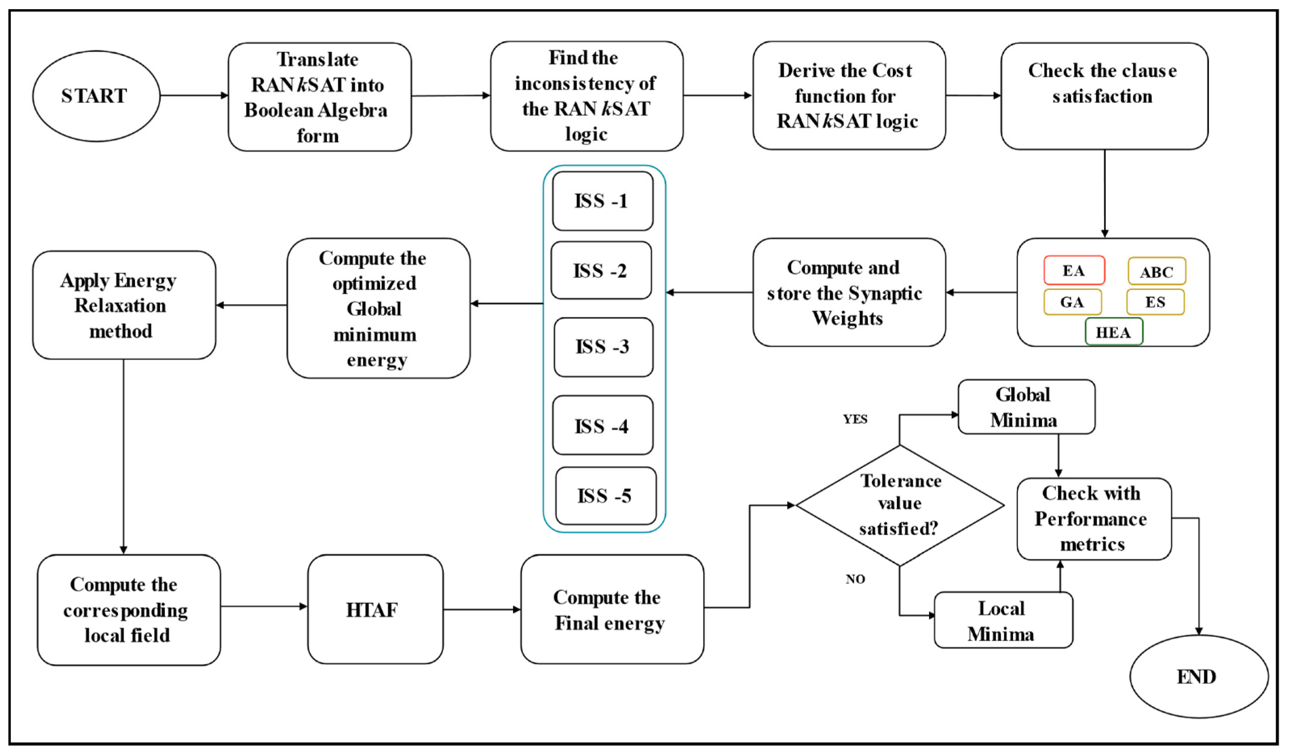
3. Random k Satisfiability in Discrete Hopfield Neural Network (DHNN)

The Discrete Hopfield Neural Network (DHNN) is a type of ANN referred to as a feedback network. In most cases, feedback refers to the output being sent back into the network. DHNN used one of the most successful storage techniques, termed content addressable memory (CAM) processes with binary/bipolar threshold units that are guaranteed local minimum convergence. DHNN is a network with no hidden layers and comprises interconnected neurons where the neurons are updated asynchronously. Here, we used the asynchronous neuron adaption of Theorem 1 to represent the DHNN units in bipolar values (1, −1). Theorem 1 shows that DHNN operated asynchronously concerning its condition.

Theorem 1.

All networks described by (8) in randomized asynchronous mode will fall into a network gap with a probability of one when starting at an initial state in search space [32].

$$S_i=\{\begin{array}{l}1,\hspace{1em}if {\displaystyle \sum _j^n{W}_{abc}{S}_b{S}_c\ge U_p}\\ -1,\hspace{1em}otherwise\end{array}$$

(8)

From (8), $W_{abc}$ is the synaptic weight from unit $a$ to $c$. $S_b$ is the current state of the unit $b$, and $U_p$ is the pre-defined threshold. Several studies [33,34] defined $U_p=0$ to verify that the DHNN always lead to a decrease in energy monotonically. The synaptic weight between neurons $a$ and $b$ corresponds to the intensity of connections between two neurons. Likewise, the neuron connections are approached $W_{ab}$ as $W_{abc}^{\left(3\right)}={\left[W_{abc}^{\left(3\right)}\right]}_{n\times n}$ with ${\left[U_p\right]}_{n\times 1}={\left[U_1,U_2,U_3,\dots ,U_n\right]}^T$. The computation of the cost function $C_{{\alpha }_{\mathrm{RAN}3\mathrm{SAT}}^k}$ in DHNN is significant to decrease the logical inconsistency of ${\alpha }_{\mathrm{RAN}3\mathrm{SAT}}^k$ $\left(C_{{\alpha }_{\mathrm{RAN}3\mathrm{SAT}}^k}=0\right)$. The design of $C_{{\alpha }_{\mathrm{RAN}3\mathrm{SAT}}^k}$ Equations (9) and (10) that adapts all forms of logic combinations ${\alpha }_{\mathrm{RAN}3\mathrm{SAT}}^k$ is as follows.

$$C_{{\alpha }_{\mathrm{RAN}3\mathrm{SAT}}^k}=\frac{1}{8}{\displaystyle \sum _{i=1}^w\left({\displaystyle \prod _{j=1}^3{L}_{ij}}\right)}+\frac{1}{4}{\displaystyle \sum _{i=1}^v\left({\displaystyle \prod _{j=1}^2{L}_{ij}}\right)}+\frac{1}{2}{\displaystyle \sum _{i=1}^u\left({\displaystyle \prod _{j=1}^1{L}_{ij}}\right)}$$

(9)

$$L_{ij}=\{\begin{array}{l}\frac{1}{2}(1-S_{i_1}), if \neg i_1\\ \frac{1}{2}(1+S_{i_1}), otherwise\end{array}$$

(10)

where $S_{i_1}$ is the neuron state where $i_1\in \left\{1,-1\right\}$. The probability for consistent interpretation is expressed in (11).

$$P\left(C_{{\alpha }_{\mathrm{RAN}3\mathrm{SAT}}^k}=0\right)={\displaystyle \prod _{i=1}^3{\left(1-\frac{1}{2^i}\right)}^{\chi \left(J_i^{(k)}\right)}}$$

(11)

where $\chi (J_i^{(k)})$ is the number of $J_i^{(k)}$ clauses. The fundamental goal of using ${\alpha }_{\mathrm{RAN}3\mathrm{SAT}}^k$ DHNN is to successfully minimize the cost function $C_{{\alpha }_{\mathrm{RAN}3\mathrm{SAT}}^k}$, which aids in finding proper synaptic weights and producing a good energy profile. Since ${\alpha }_{\mathrm{RAN}3\mathrm{SAT}}^k$ has a zero-cost function, it provides a satisfied interpretation (all clauses give truth value).

The local field of DHNN is given by (12). $S_i\left(t\right)$ is symbolized as the final state of neurons, whereby $W_{abc}^{(3)}, W_{ab}^{(2)}, W_a^{(1)}$ are for third, second and first-order, respectively. The Hyperbolic Tangent Activation Function (HTAF) was used in the testing phase dynamics of DHNN to enable the convergence of final neuron states while avoiding neuron oscillation [17]. The local field of our proposed model is formulated in (12) and (13) as follows:

$$h_p\left(t\right)={\displaystyle \sum _{c=1,c\ne b}^n{\displaystyle \sum _{b=1,b\ne c}^n{W}_{abc}^{(3)}}}{S}_b{S}_c +{\displaystyle \sum _{b=1,b\ne a}^n{W}_{ab}^{(2)}}{S}_b+W_b^{(1)}$$

(12)

$$S_i\left(t\right)=\{\begin{array}{rr}1,& {\displaystyle \sum _{c=1,c\ne b}^n{\displaystyle \sum _{c=1,c\ne b}^n{W}_{abc}^{(3)}{S}_b{S}_c}}+{\displaystyle \sum _{b=1,b\ne a}^n{W}_{ab}^{(2)}{S}_b}+W_a^{(1)}\ge 0\hfill \\ \hfill -1,& {\displaystyle \sum _{c=1,c\ne b}^n{\displaystyle \sum _{c=1,c\ne b}^n{W}_{abc}^{(3)}{S}_c{S}_b}}+{\displaystyle \sum _{b=1,b\ne a}^n{W}_{ab}^{(2)}{S}_b}+W_a^{(1)}<0\hfill \end{array}$$

(13)

Here, Equation (12) is the overall formulation of the local field for ${\alpha }_{\mathrm{RAN}3\mathrm{SAT}}^k$ and (13) is a piecewise function of the generated final state of the neuron according to the value of (8). In this paper, Wan Abdullah (WA) method is used to compare Equation (9) with Equation (14), which is noted as an energy function $H_{{\alpha }_{\mathrm{RAN}3\mathrm{SAT}}^k}$. Therefore, the WA method is an ideal method to find $W_{abc}$ in the case of ${\alpha }_{\mathrm{RAN}3\mathrm{SAT}}^k$ DHNN.

$$\begin{array}{ll}{H}_{{\alpha }_{\mathrm{RAN}3\mathrm{SAT}}^k}=& -\frac{1}{3}{\displaystyle \sum _{a=1,a\ne b\ne c }^n{\displaystyle \sum _{b=1,a\ne b\ne c }^n{\displaystyle \sum _{c=1,a\ne b\ne c}^n{W}_{abc}^{\left(3\right)}{S}_a{S}_b{S}_c}}}\\ & -\frac{1}{2}{\displaystyle \sum _{a=1,a\ne }^n{\displaystyle \sum _{b=1,a\ne b}^n{W}_{ab}^{\left(2\right)}{S}_a{S}_b}} -{\displaystyle \sum _{a=1}^n{W}_a^{\left(1\right)}{S}_a}\end{array}$$

(14)

and then the value $H_{{\alpha }_{\mathrm{RAN}3\mathrm{SAT}}^k}$ attains the absolute final energy, and the minimum energy $H_{{\alpha }_{\mathrm{RAN}3\mathrm{SAT}}^k}^{min}$ is gained from ${\alpha }_{\mathrm{RAN}3\mathrm{SAT}}^k$ that reduced monotonically [24]. Hence, $H_{{\alpha }_{\mathrm{RAN}3\mathrm{SAT}}^k}^{min}$ is calculated by (15).

$$H_{{\alpha }_{\mathrm{RAN}3\mathrm{SAT}}^k}^{min}=-\frac{a\left({\psi }_i^3\right)+2\left(b\left({\psi }_i^2\right)\right)+4\left(c\left({\psi }_i^1\right)\right)}{8}$$

(15)

and ${\psi }_i^1, {\psi }_i^2, {\psi }_i^3 \in J_i^{\left(k\right)}$ and $c,b,a$ symbolize the numbers for 1 literal, 2 literals and 3 literal clauses in ${\alpha }_{\mathrm{RAN}3\mathrm{SAT}}^k$.

Finally, Equation (16) can analyze the final neuron states’ quality by distinguishing between the global and local minimum solutions. Notably, if (16) is satisfied, and the final neuron states will attain global minima solution; else, it would be trapped in a local minima solution.

$$\left|H_{{\alpha }_{\mathrm{RAN}3\mathrm{SAT}}^k}-H_{{\alpha }_{\mathrm{RAN}3\mathrm{SAT}}^k}^{min}\right|\le \tau$$

(16)

where $\tau =0.001$ is the pre-defined value, which is known as the tolerance value. Algorithm 1 summarizes the steps of DHNN-RANkSAT through the pseudo-code below.

Algorithm 1 The pseudocode of DHNN-RANkSAT in the logic phase.
1	Start
2	Set the initial parameters, maximum combination (COMBMAX) = 1, trial number
3	Initialize the neuron to each variable consisting of $S_i\in \left[S_1,S_2,S_3,\dots S_n\right]$
4	While$(i\le trial)$
5	Forming initial states by using Equation (8)
	[TRAINING PHASE]
6	Define cost function $C_{{\alpha }_{\mathrm{RAN}3\mathrm{SAT}}^k}$ by using Equation (9)
7	For $S_i\in \left[S_1,S_2,S_3,\dots S_n\right]$ do
8	Check clauses satisfaction by Equation (9)
9	If$C_{{\alpha }_{ \mathrm{RAN}3\mathrm{SAT}}^{ k}}=0$
10	$S_i$$\to$Satisfied
11	Else
12	$S_i$$\to$ Unsatisfied
13	End For
14	Calculate synaptic weights by using the Wan Abdullah method.
15	Compute the $H_{{\alpha }_{\mathrm{RAN}3\mathrm{SAT}}^k}$ by using Equation (14).
	[TESTING PHASE]
16	Local field computation to find the final state by using Equation (12)
17	For ($i\le trial$)
18	End For
19	Compute the $H_{{\alpha }_{\mathrm{RAN}3\mathrm{SAT}}^k}^{\min }$ by using Equation (15)
20	Calculate the final energy with tolerance value.
21	Check If it is Global minimum energy or local minimum energy
22	If$|H_{P_{\mathrm{RAN}3\mathrm{SAT}}}-H_{P_{\mathrm{RAN}3\mathrm{SAT}}}^{\min }|\le \mathrm{Tolerance}$
23	Assign Global minimum energy
24	Else
25	Assign local minimum energy
26	End

The schematic diagram for DHNN-RANkSAT is shown in Figure 1 where the RANkSAT represents k = 3, 2. In this diagram, the red line represents the third-order clauses, and the purple line denotes the second-order clauses, respectively. Within each main block, the pink, orange and blue colored lines illustrate the connection of each neuron. The energy filter represents whether it aligns with the tolerance value or not. The output of the diagram depicts that either it can achieve the global minimum or a local minimum energy.

4. Proposed Multi-Objective Functions for DHNN

This paper proposes several objective functions that ensure accuracy and diversity. The foremost concept is to introduce the multi-objective nature in our proposed work so that we can maximize the fitness value as well as create diversity in the logical rule with enhancing the storage capacity of DHNN. The potentiality of the proposed multi-objective concept is that it embeds all the objectives in a perfect alignment maintaining the RANkSAT strategy. Analyzing the accuracy and diversity would be an inventive study of higher-order RANkSAT representation.

Consequently, the question arises: How can an algorithm achieve both accuracy and diversity at the same flow? To answer this question, a satisfactory equilibrium needs to be set up with two fundamental concepts- exploration and exploitation of the search space that can balance with accuracy and diversity of the proposed algorithm. Additionally, researchers ponder that those algorithms/metaheuristics search methods can reach better performance if the exploration and exploitation of the search space maintain the appropriate balance [35].

Researchers needs to know that accuracy and diversity are also not in the same pair, and to achieve accuracy and diversity in an algorithm, a multi-objective concept needs to comply to achieve the trade-off between diversity and accuracy also. To find the novelty of our proposed work, we need to investigate the performance and robustness of optimum solutions. Here, the main novelty of our proposed work optimizes three objectives: (i) the maximum fitness, (ii) diversity ratio and (iii) k ideal solution strings. Mathematically, the proposed multi-objective functions can be generalized as:

$$f(F_{\max ,},\gamma ,S_{\max }^{(i)})$$

Now these three objective functions are explained below in detail.

4.1. Maximum Fitness Value

To achieve maximum fitness, the fitness value is estimated through certain steps of the individual operations strategy of an algorithm. Strings that obtain the highest fitness value are selected for the next stage. If a certain number of strings of an algorithm cannot achieve the highest fitness value, it needs to undergo the trial again from the beginning of its mechanism. The illustration of the general form of maximum fitness value of RANkSAT by summing up the fitness value of each order of clauses is shown below:

$$F_{\max }={\displaystyle \sum _{i=0}^p{C}_i^{(3)}+{\displaystyle \sum _{i=0}^q{C}_i^{(2)}+{\displaystyle \sum _{i=0}^r{C}_i^{(1)}}}}$$

where $C_i^{(3)},C_i^{(2)},C_i^{(1)}$ are the third-order, second-order and first-order clauses of RANkSAT, respectively.

4.2. Each Clause Contains at Least One Negative State $C_i^k,k\ge 2$

The state of the literal is one of our objectives for addressing diversity in a logical rule. To ensure this objective, we include at least one negative state in each clause of RANkSAT, which will make the logical rule more diverse. In the logical diversity arrangement for RANkSAT, we focus on the literals arrangement for ${\delta }_{P_{3SAT}}$ (3SAT) and ${\delta }_{P_{2SAT}}$ (2SAT) clauses. Since ${\delta }_{P_{3SAT}}$ and ${\delta }_{P_{2SAT}}$ can create more than one possible solution, we only evaluate these clauses in our diversity calculation strategy. Note that ${\delta }_{P_{1SAT}}$ (first-order) clauses have no substitute options for clause satisfaction so it has no impact on our diversity logical strategy. Hence, the calculation of diversity in terms of logical structure for ${\delta }_{P_{3SAT}}$ and ${\delta }_{P_{2SAT}}$ is expressed as in the equation is described below:

$$\gamma ={\displaystyle \sum _{i=0}^p{C}_i^{(3)}+{\displaystyle \sum _{i=0}^q{C}_i^{(2)}}}$$

4.3. k-Ideal Solutions Strings (ISS)

In DHNN, the solution string is represented in bipolar form. This solution string is stored as an associative memory system known as Content Addressable Memory (CAM). Each solution string from the learning phase will span the initial bipolar vector and become the root of the storage. After satisfying Equations (18) and (19), the solution strings are chosen. These solution strings are known as Ideal Solution Strings (ISS). Notably, if the mechanism of an algorithm fails to achieve ideal strings, a further trial will occur from the highest fitness string reservoir. Since DHNN suffers from limited storage capacity, enhancing the storage capacity of DHNN is the real focus of our proposed HEA. Here the arrangements of Ideal strings are shown below:

$$S_{\max }^{(i)}=[S^{(1)},S^{(2)},S^{(3)},S^{(4)},S^{(5)}]$$

overall, these multi-objective functions have been written mathematically in Equations (17)–(20):

$$f(F_{\max ,},\gamma ,S_{\max }^{(i)})$$

(17)

Subject to

$$(\mathrm{For} \mathrm{Fitness}) F_{\max }={\displaystyle \sum _{i=0}^p{C}_i^{(3)}+{\displaystyle \sum _{i=0}^q{C}_i^{(2)}+{\displaystyle \sum _{i=0}^r{C}_i^{(1)}}}}$$

(18)

$$(\mathrm{For} \mathrm{Diversity}) \gamma ={\displaystyle \sum _{i=0}^p{C}_i^{(3)}+{\displaystyle \sum _{i=0}^q{C}_i^{(2)}}}$$

(19)

$$(k\text{-}\mathrm{Ideal} \mathrm{Solution} \mathrm{Strings}) S_{\max }^{(i)}=[S^{(1)},S^{(2)},S^{(3)},S^{(4)},S^{(5)}]$$

(20)

where $C_i^{(3)},C_i^{(2)},C_i^{(1)}$ are the third-order, second-order and first-order clauses and $\gamma$ represent the combination of a minimum number of negative states in each clause of RANkSAT and $S^{(1)}$,…, $S^{(5)}$ are the total (05) CAM or Ideal solution strings, respectively.

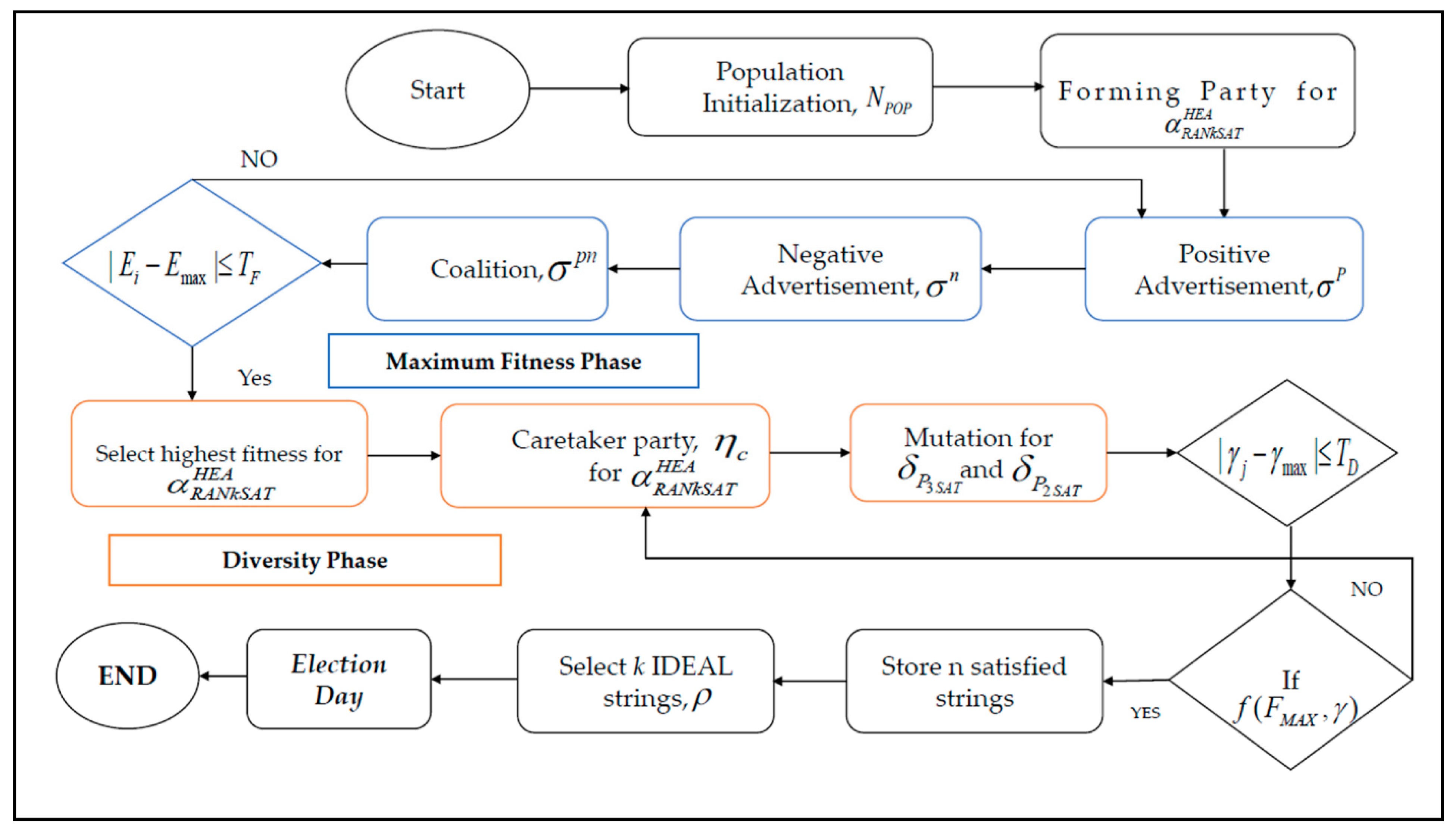
5. Proposed Hybrid Election Algorithm (HEA)

The key motivation of a hybridized algorithm is that it can cover a wide range of solutions and generate several distinct computations. Generally, metaheuristics have two segments that allow them to carry out the optimization process. These segments include the exploration of search spaces to identify potential regions of good solutions, as well as the exploitation phase, which intensifies the search for the best regions to find better solutions [36].

Moreover, a logical representation that follows non-systematic logical expressions, such as RANkSAT, is more effective in a hybrid metaheuristic for avoiding overfitting solutions. In this context, the novel Hybrid Election Algorithm (HEA) is introduced, a type of social-political metaheuristics that combines evolutionary algorithms and swarm intelligence operations, which occupy both exploration and exploitation in a proper manner. There are no recent works that employ achieving the highest fitness value along with creating diversity in the logical rules. The core reason for addressing HEA in our paper is achieving maximum fitness value and simultaneously creating diversity in the logical rules in the same pair.

In terms of optimization, HEA introduced another efficient optimizer that can improve the local solutions. Following this, the characteristics of RANkSAT can rely heavily on the HEA because of its effective and robust mechanism. The HEA is utilized in this paper to find the best RANkSAT assignment that minimizes the cost function during the training phase of DHNN. The model is elucidated with detailed information in the next section. The procedure of the Hybrid Election Algorithm in DHNN-RANkSAT is explained in Section 5.1, Section 5.2, Section 5.3, Section 5.4 and Section 5.5

5.1. Initialization

The population $\left(N_{POP}\right)$ of individuals consisting of voters and candidates includes potential solutions of the search space of ${\alpha }_{\mathrm{RAN}3\mathrm{SAT}}^{HEA}$ is generated randomly. Let $S_i=\left\{S_1,S_2,S_3,\dots S_N\right\},S_i\in \left(1,-1\right)$ is initialized. The state of each individual is noted as 1(TRUE) and −1(FALSE), which aligns with the possible instances ${\alpha }_{\mathrm{RAN}3\mathrm{SAT}}^{HEA}$. Consider the search space of ${\alpha }_{\mathrm{RAN}3\mathrm{SAT}}^{HEA}$ being $S_{{\alpha }_{\mathrm{RAN}3\mathrm{SAT}}^{HEA}}=\left\{S_1,S_2,S_3,\dots S_{2^n}\right\}$.

5.2. Eligibility Assessment

All randomized instances must undergo eligibility/fitness function assessment. There will be a reward for each of the correct instances that results in a satisfying RANkSAT clause. During the eligibility/fitness assessment process, the number of achieved clauses is used to determine the eligibility of the individuals. The eligibility or fitness value can be determined from Equation (21).

$$f_{L_j}={\displaystyle \sum _{i=1}^{NC}{C}_i^{\left(k\right)}}, k=1,2,3$$

(21)

$$C_i^{\left(k\right)}=\{\begin{array}{l}0, False\\ 1, True\end{array}$$

(22)

where $C_i^{\left(k\right)}$ means the order of RANkSAT clauses. The aim is to increase the value of the eligibility/fitness function or decrease the value of the cost function.

5.3. Initial Formation of the Parties

In this stage, the solution space is divided into $N_{party}$ parties. Then, the process of calculation of voters for each party can be written in Equation (23).

$$N_j=\frac{N_{Pop}}{N_{Party}}, j=1,2,3,4$$

(23)

where $N_{Pop}$ is the size of the population. Equation (23) is used to determine the eligibility of each instance (voters or candidates). In each party $j$, the prospective solution with the highest eligibility value is elected as a candidate $L_w$. The remaining the instances are attached as the voter $V_w$ of the candidate. Then, the correlation distance function (CorD) between the candidate $L_w$ and the voter $V_w$ was expressed in Equation (24).

$$CorD(f_{L_w,}{f}_{V_w})=f_{L_w}-f_{V_w}$$

(24)

5.4. Advertisement Campaign

After organizing the initial parties, we select the initial candidate with the highest fitness solution in each party. The main distinction between standard EA and the proposed HEA is largely due to the progress made in this advertising campaign. Next, each candidate will launch its advertising campaign, which will consist of four steps: positive advertisement, negative advertisement, coalition, and newly affiliated- another effective step is the caretaker party. Hence, these sub-steps of the advertisement campaign are explained below.

5.4.1. Positive Advertisement

The candidate will reveal their plans during this stage and attempt to sway voters voting selections. Hence, the number of voters who the candidate will influence is given as follows:

$$N_{A_j}=N_j{\sigma }^p, j=1,2,3,4$$

(25)

where ${\sigma }^p$ is a positive advertisement rate ${\sigma }^p\in \left[0,0.5\right]$. The reasonable effect between the candidate and the voter is expressed as the eligibility correlation distance coefficient by (26).

$${\omega }_{v^i}=\frac{1}{1+CorD(f_{L_w,}{f}_{V_w})}$$

(26)

Each influenced voter $v^i$ will determine the number of neuron states that can update based on the following Equation (27).

$$S_{v^i}=N_j{\omega }_{v^i}$$

(27)

where $N_j=3w+2v+u$ is the sum of the first, second and third-order of ${\alpha }_{\mathrm{RAN}k\mathrm{SAT}}^{HEA}$. First, the influenced voter will update the neuron state randomly according to the predetermined number. Then, the eligibility/fitness value of each of the influenced voters $v^i$ will be evaluated based on (21). In each party, there is the possibility that the influenced voter $v^i$ will replace the current candidate due to higher eligibility/fitness value.

As a result, the candidate will be replaced by the solution with the highest fitness value in order to improve the quality of the solutions in the parties (more qualified supporters). If a voter and a candidate have the same eligibility, the candidate position shall be maintained (no replacement will be made). Suppose the best solution is identified in the positive advertisement. In that case, it will continue to be a candidate in the following steps until the first iteration is completed, at which point it will be announced as the best solution in the election stage.

5.4.2. Negative Advertisement

At this point, candidates use negative advertising to try to entice supporters from other parties to their side to expand the search space. This negative campaign generally benefits popular parties because it leads to an increase in popularity. Equation (28) depicts the number of voters ($N_j$) candidates can attract from other parties voters ($N_{A_j}$) with the highest fitness value.

$$N_{A^{\ast j}}={\sigma }^n(N_j-N_{A_j})$$

(28)

where $A^{\ast j}$ are the voters from other parties, and ${\sigma }^n$ is a negative advertisement rate ${\sigma }^n\in [0,0.5]$. The correlation or similarity belief between the voters and the candidates is similar to Equation (29).

$$CorD(f_{L_w,}{f}_{V_{\ast w}})=f_{L_w}-f_{V_{\ast w}}$$

(29)

The reasonable effect from the candidate to the voter from another party is defined based on the eligibility distance correlation coefficient ${\omega }_{v^{\ast i}}$.

$${\omega }_{v^{\ast i}}=\frac{1}{1+CorD(f_{L_w,}{f}_{V_{\ast w}})}$$

(30)

Each influenced voter $v^{\ast i}$ will determine the number of neuron states, which can be updated based on the following Equation (31).

$$S_{v^{\ast i}}=N_j{\omega }_{v^{\ast i}}$$

(31)

By using Equation (26), we can calculate the eligibility of the new supporters. Again, if a voter has a fitness value greater than the candidate, the candidate will be replaced by this voter.

5.4.3. Coalition

During this stage, parties collaborate and establish a coalition in order to explore additional areas in the search space ${\alpha }_{\mathrm{RAN}k\mathrm{SAT}}^{HEA}$. The processes and formulations used in the coalition stage were the same as in the previous strategy. First, the two parties will be randomly combined to determine the new candidate after this merger. To begin, use Equation (22) to determine the eligibility distance function and distance coefficient. Then, using Equation (23), specify the number of variables that need to be updated in each voter from this united party. The fitness values of all voters have now been updated. Finally, a comparison is made between the voters’ fitness and previous candidates’ fitness. This will be elected if the old candidate still has the highest fitness value in the next stage. However, if other circumstances arise, such as a voter having a higher fitness rating than the previous candidate. This fittest voter will be a new candidate who will face off against another political party.

5.4.4. Caretaker Party

After completing the traditional coalition stage, the accuracy of the proposed model is tested. If this proposed model satisfies its accuracy (by finding k strings that achieve the highest fitness value), we can proceed to the next phase, known as the diversity phase. This diversity phase generates the ability to create the ‘best pool’ of instances where voters can only stay with the maximum fitness value. This ‘best pool’ is named the Caretaker party. In this stage, those who achieved the highest fitness value were selected for this pool. Mainly Caretaker party takes care of all of its best strings. Therefore, the dynamic stairs enhance the diversity of the proposed HEA mechanism model. The selection process for choosing the highest fitness value can be calculated by Equation (28).

$$C_p^{best}=\theta f_{L_j}$$

(32)

where $\theta =[0.1,0.4]$ is the ratio of the achieved maximum fitness value.

The mutation insertion concept is also utilized in this Caretaker party to improve its diversity, which creates a new dimension in the study of the proposed HEA model. Notably, the Caretaker party emphasizes the exploitation mechanism. Thus, it is better to choose such a type of mutation insertion, which can choose randomly with a more localized search. Moreover, the general mutation is muted randomly while there is no mechanism to detect unsatisfied clauses and inclusion of positive/negative states. In this context, we exploit shift mutation that works by shifting a randomly chosen frontier between two adjacent clauses by one/ single step, either to the right to the left or vice versa [37]. Shift mutation not only focuses on non-satisfied clauses but also focuses on the inclusion of positive-negative states combination in each clause. In retrospect, the Shift mutation operator essentially provides HEA with local search capability; a phenomenon called intensification. However, shift mutation is a more localized search operation than swap mutation.

Hence, the condition of Equation (32) is satisfied; the fittest voters are moved to the next stage for the participating final round—‘Election Day’.

5.5. The Election Day

The best solution (the candidate) in each party will be tested at this stage. Then, this solution will be announced as the optimal solution if it has attained the maximum fitness value with desired logical states (at least one negative state in the solution string). Otherwise, a second iteration will be carried out. After that, the procedures will be repeated until all conditions (from Equations (23)–(32)) have been met.

Meanwhile, we provide a real example in Appendix A that may guide how voters and candidates represent the value of a Party. Now, we present the pseudocode in the Algorithm 2 and sketch the total flowchart in Figure 2, of our proposed Hybrid Election Algorithm (HEA) below:

Algorithm 2 Pseudocode for proposed Hybrid Election Algorithm.
1	Start
2	Initialize the population $N_{POP}$ consisting of $S_i\in \left\{S_1,S_2,S_3,\dots S_{N_{POP}}\right\}$
3	While $i\le trial$
4	Forming initial parties by using Equation (23)
5	For$J\in \left\{1,2,3,\dots N_{Party}\right\}$ do
6	Calculate the similarity between the voters and the candidates by using Equation (24)
7	End For
8	[Positive Advertisement]
9	For $S_i\in \left\{1,2,3,\dots N_{s_i}\right\}$ do
10	Evaluate the number of voters by using Equation (25)
11	Evaluate the reasonable effect from the candidate ${\omega }_{v^i}$ by using Equation (26)
12	Update the neuron state according to Equation (27)
13	If $f_{v_i^j}>f_{L_j}$
14	Assign $v_i^j$ as new $L_j$
15	Else
16	Remain $L_j$
17	End For
	Negative Advertisement]
18	For $S_i\in \left\{1,2,3,\dots N_{v_j^{\ast }}\right\}$ do
19	Evaluate the similarity between the voters from the other party and the candidate from Equation (28)
20	Evaluate the reasonable effect from the candidate ${\omega }_{v_i^{\ast }}$ and update the neuron state by using Equation (30)
21	If $f_{v_i^{\ast }}>f_{L_j}$
22	Assign $v_i^{\ast }$ as new $L_j$
23	Else
24	Remain $L_j$
25	End For
26	[Coalition]
27	For $S_i\in \left\{1,2,3,\dots N_{v_j^{\ast }}\right\}$ do
28	Evaluate the similarity between the voters from the other party and the candidate from Equation (29)
29	Evaluate the reasonable effect from the candidate ${\omega }_{v_i^{\ast }}$ and update the neuron state by using Equation (30)
30	If $f_{v_i^{\ast }}>f_{L_j}$
31	Assign $v_i^{\ast }$ as new $L_j$
32	Else
33	Remain $L_j$
34	End For
35	End While
	[Caretaker Party]
36	For $S_i\in \left\{1,2,3,\dots N\right\}$ do
37	//Input Mutation operator//
38	If $f_{v_i^N}>f_{L_j}$
39	//Choose Five Highest fitness candidates//
40	Assign $5v_i^{\ast }$ as new $5L_j$ (Select five voters as five new candidates)
41	Else
42	Remain $5L_j$ (Five new candidates)
43	End For
44	Return Output the Five final neuron states
45	End
46	End While
47	Return Output the final neuron state

5.6. Model Reproducibility

The same experiments need to be conducted to reproduce a framework with the model DHNNRANkSAT-HEA repeatedly on certain data sets or obtain the same results. Specific factors should be considered as below:

i.

The logical presentation must be RANkSAT for k = 3, 2 structure where the threshold iteration is set at 100 to distinguish the maximum capacity of the presented algorithms.

ii.

To achieve the optimal synaptic weight in the training phase, the WA method is utilized. According to [24], the WA method is more stable than Hebbian learning. It is worth mentioning that different logic operators have different capabilities in producing negative literal.

6. Experimental Setup

In this section, we verify the effectiveness of the proposed DHNNRANkSAT-HEA model during the training phase. This experiment considers multi objectives concept, which determines the proposed model achieves the highest fitness value, generates a correct number of negative literals in each clause and produces ideal solution strings. To guarantee the reproducibility of the experiment, we set up our experiment as follows:

6.1. Simulation Design and Simulation Datasets

All the simulations will be conducted on the same features to avoid biases during experimentation. The features are as follows:

i.

Device Setting: The simulation was run on the device with a 4 GB RAM Intel Core i5 processor with a 64-bit Windows 10 Operating System where the CPU time threshold for data generation will be 24 h. The proposed model was implemented and analyzed by using Dev C++ version 5.11.

ii.

SAT Configuration: The number of neurons ranging from $10\le NN\le 120$. The logical framework is based on third and second-order logic. Therefore, the clauses in a logical structure are chosen randomly.

iii.

Proposed HEA Code (Online): The source code of the proposed model can be found at the mentioned link: https://bit.ly/3PEcYl4 (25 May 2022)

The experiment will be conducted with simulated data produced at random by the proposed model. The simulated data set’s elements are strings of bipolar values that are (−1, 1) based on the RANkSAT for k = (3, 2) structure. Simulation data sets are often utilized in testing and evaluating the capabilities of a new proposed SAT in DHNN, according to research by [12,14,15,23,24]. As a result, when applied to real-life data sets, the results of the simulated data set will project the usefulness of the proposed model.

6.2. Parameters Assignment

Table 2. Parameter list for the DHNNRANkSAT-HEA model.

Parameter	Parameter Value
$\mathrm{Number} \mathrm{of} \mathrm{Neurons} (NN$)	$10\le NN\le 120$ [14]
$\mathrm{Number} \mathrm{of} \mathrm{Learning} (NH)$	100 [23]
$\mathrm{Number} \mathrm{of} \mathrm{Trials} (NT)$	100 [23]
$\mathrm{Neuron} \mathrm{Combinations} (NCM)$	100 [14]
CPU time threshold	24 h [12]
Order of Clauses	$Z_i^{(3)},Z_i^{(2)}$ [14]
Total Number of Clauses	$1\le n(Z_i^{(3)}+Z_i^{(2)})\le 50$ [14]
$\mathrm{Size} \mathrm{of} \mathrm{Population} (N_{POP})$	120 [21]
$\mathrm{Number} \mathrm{of} \mathrm{Parties} (N_{Party})$	4 [21]
$\mathrm{Positive} \mathrm{advertisement} ({\sigma }^P)$	0.5 [21]
$\mathrm{Negative} \mathrm{advertisement} ({\sigma }^n)$	0.5 [21]
Diversity of logical rules (in Percentage)	40%
Activation Function	Hyperbolic Tangent Activation Function [17]
Neuron state Initialization (Training Phase)	Random
Testing Phase Neuron State	Random
Number of Learning Iterations	100 [24]

,

Table 3. List of parameters used in DHNNRANkSAT-EA, DHNNRANkSAT-GA and DHNNRANkSAT-ABC.

Parameter	Parameter Value
$\mathrm{Number} \mathrm{of} \mathrm{Neurons} (NN$)	$10\le NN\le 120$ [14]
$\mathrm{Number} \mathrm{of} \mathrm{Learning} (NH)$	100 [23]
$\mathrm{Number} \mathrm{of} \mathrm{Trials} (NT)$	100 [23]
$\mathrm{Neuron} \mathrm{Combinations} (NCM)$	100 [14]
$\mathrm{Size} \mathrm{of} \mathrm{Population} (N_{POP})$	120 [23]
$\mathrm{Number} \mathrm{of} \mathrm{Parties} (N_{Party})$	4 [24]
$\mathrm{Positive} \mathrm{advertisement} ({\sigma }^P)$	0.5 [23]
$\mathrm{Negative} \mathrm{advertisement} ({\sigma }^n)$	0.5 [23]
Neuron state Initialization (Training Phase)	Random
Testing Phase Neuron State Initialization	Random
Number of Learning Iterations	100 [24]

and

Table 4. List of parameters used for DHNNRANkSAT-ES.

Parameter	Parameter Value
$\mathrm{Number} \mathrm{of} \mathrm{Neurons} (NN$)	$10\le NN\le 120$ [14]
$\mathrm{Number} \mathrm{of} \mathrm{Learning} (NH)$	100 [15]
$\mathrm{Number} \mathrm{of} \mathrm{Trials} (NT)$	100 [17]
$\mathrm{Neuron} \mathrm{Combinations} (NCM)$	100 [23]
Neuron state Initialization (Training Phase)	Random
Testing Phase Neuron State Initialization	Random
Number of Learning Iterations	100 [24]

show the parameter control considered in this study. The number of ideal strings will be set to 5. To evaluate the final energy of DHNN, the tolerance value will be 0.001 [23]. DHNN will undergo relaxation by applying the Sathasivam relaxation method. The relaxation rate is set to 3 because a lower value will cause the neuron to exchange information and relax to global minimum energy. All parameters are tuned offline. Since the parameter values are identified before applying the algorithm.

The optimal parameter setting founded by the tuning process is used in solving problems and these parameter values remain unchanged during the simulation run. Moreover, our proposed algorithm is following the work of [12,14,15,21,22,23,24] and to make a fair comparison, all the parameter values should be automatically tuned with the mentioned studies. Otherwise, strongly impairing a non-tuned algorithm could mislead the conclusion from the proposed algorithm [38]. The training and testing phase will randomly initialize the neuron state. Table 2, Table 3 and Table 4 summarize the parameter assignments.

7. Performance Evaluation Metrics

7.1. Numerical Calculation of Storage Capacity $({\beta }_C)$

An associative memory system or CAM is formed as a ‘storage box’ for the Discrete Hopfield Neural Network. Discovering multiple CAM in a single model should increase the storage capacity of DHNN. In the general simulation strategy, each solution string is stored in a single CAM, which is the basic nature of DHNN. Interestingly, more solution strings will be approached in our proposed simulation approach.

The string that satisfies both maximum fitness and diversity phase is called ‘Fully Satisfied Strings $(\mu )$’. In a single simulation, if the model generates at least five (05) full satisfied strings $(\mu )$ are considered “Ideal Solution Strings $(\rho )$”. To predict the storage capacity via CAM, it is necessary to find the relation between full satisfied strings $(\mu )$ and Ideal solution strings $(\rho )$. Equation (33) explains how our model achieves its destination in terms of the storage capacity of DHNN:

$${\beta }_C=\{\begin{array}{l}1, When \mu \le \rho \\ 0, Otherwise\end{array}$$

(33)

where the value of ${\beta }_C$ corresponding to 1 means that the model achieved its full storage requirement regarding CAM.

7.2. Diversity Calculation Strategy

In a multi-objective function, diversification of a model is a vital criteria. In a population-based metaheuristic, the diversity metric is a state-of-the-art metric that can assist in exploration and exploitation assessment that can find the real solutions for real-world applications [39]. The calculation procedure for diversity depends on the various parameters and relevant objects. Here, in our paper, we calculate the diversity ratio in a logical structure. The maximum diversity and the calculation of the diversity rate of a logical structure are shown in Equations (34) and (35).

$$\mathrm{Maximum} \mathrm{Diversity}, D_{\max }=\xi (3m+2n)$$

(34)

where $\xi =0.40,$ means that the total diversity of the logical rule will be calculated from 40%, $m=$ Number of 3SAT clauses and $n=$ Number of 2SAT clauses.

$$\mathrm{Calculation} \mathrm{of} \mathrm{Proposed} \mathrm{Diversity} \mathrm{rate}=\frac{{\nu }_A}{{\nu }_T}\times 100\%\ge 40\%$$

(35)

$v_A$ = Achieved Number of States, and $v_T$ = Target Number of States.

7.3. Mean Absolute Error

During the training and testing phase, the standard error based on the average difference between the computed fitness value and the expected fitness value of the DHNN-RANkSAT model process is acquainted with Mean Absolute Error (MAE). According to [40], MAE appears to be a trustworthy statistic in measuring the correctness of a model. Thus, the calculation process for MAE in DHNN-RANkSAT (Training and Testing phase) is recrafted as follows:

$$MAE=\frac{1}{n}|f_{\max }-f_i|$$

(36)

where $f_i$ refers to the obtained fitness value, $f_{\max }$ is the maximum number of fitness values, and $n$ denotes the number of iterations that corresponds to the RANkSAT logic.

7.4. The Ratio of Global Solutions (RGS)

Energy analysis can be carried out by observing the quality of the solutions to determine if it is global minima solutions that correspond to global minimum energy. The ratio of global minima solutions can be calculated as

$$RGS=\frac{1}{NT\ast NCM}{\displaystyle \sum _{i=1}^{n}N{G}_{H_{P_{\mathrm{RAN}k\mathrm{SAT}}}}}$$

(37)

where $NG$ means the number of global minimum energy by the proposed model.

7.5. Similarity Index (SI)

This study will use a similarity analysis metric to compare the final states obtained using DHNN-RANkSAT. In theory, the majority of neuron states recovered by DHNN have reached global minimum energy. Inspired by the work of [23], this similarity metric will be extended to examine the RANkSAT logical representation form of the network final states. The comparison is performed by taking the benchmark states $S_{\max }^i$ with the states attained by the network $S^i$. The formula of the general comparison of the benchmark state and final state is given as in Equation (39):

$$C_{S_{\max }^i,S^i}=\left\{(S_{\max }^i,S^i);i=1,2,\dots n\right\}$$

(38)

The standard specification variables can be defined by considering the following domains:

• $l$ refers to the total number of occurrences for $(S_{\max }^i=1,S^i=1)$ in $C_{S_{\max }^i,S^i}$.
• $m$ refers to the total number of occurrences for $(S_{\max }^i=1,S^i=-1)$ in $C_{S_{\max }^i,S^i}$.
• $n$ refers to the total number of occurrences for $(S_{\max }^i=-1,S^i=1)$ in $C_{S_{\max }^i,S^i}$.
• $o$ refers to the total number of occurrences for $(S_{\max }^i=-1,S^i=-1)$ in $C_{S_{\max }^i,S^i}$.

In this paper, we suggest a variant of the similarity index called the Gower–Legendre similarity index (GLI) that considers negative co-occurrences, with a particular emphasis on positive-negative states [41]. The Gower–Legendre similarity index is adjusted in this study to account for the similarity between the simulation of final states $S^i$ and the benchmark final states $S_{\max }^i$.

$$GLI=\frac{lo}{l+0.5(m+n)+o}$$

(39)

7.6. Total Neuron Variation (TNV)

The Total Neuron Variation ($TNV$) of the DHNN model is the number of solutions that are formed in each neuron combination, and this is calculated by (40) and (41):

$$TNV={\displaystyle \sum _{V=1}^{\lambda }{G}_V}$$

(40)

$$G_{V+1}=\{\begin{array}{l}1, x_{i+1}\ne x_i\\ 0, x_{i+1}=x_i\end{array}$$

(41)

where $\lambda$ is the total number of solutions produced by the DHNN model and is the solution produced in the i-th trial.

7.7. Median Absolute Deviation (MAD)

Median Absolute Deviation (MAD) is a robust measure of variability because it uses the median as an estimate of the distribution’s center and the absolute difference rather than the squared difference [42].

$$MAD=Median(|x_i-\overline{x}|)$$

(42)

Here, $x_i$ is the refers to each value while $\overline{x}$ means the average value that corresponds to the RANkSAT models.

7.8. Friedman Statistical Analysis (F_d)

Friedman statistical analysis is used to find significant differences in the output of two or more algorithms simulated data. By computing the ranking of observed results for each metaheuristic, the Friedman test can be used to compare several methods. The general form for computing the Friedman test is given in Equation (43) [43].

$$F_d=\frac{12N}{K(K+1)}\left({\displaystyle \sum _j^{}{R}_j^2-\frac{K{(K+1)}^2}{4}}\right)$$

(43)

where $K$ is the number of metaheuristics in the test, $j$ represents its associative index, $N$ is the number of runs, and $R_j$ stands for the average rank of each algorithm. In addition, the distribution of the p-value is according to Chi-Squared distribution with $(K-1)$ degree of freedom. It is common to declare a result as a significant one if the p-value is less than 0.05 or 0.01 [44].

7.9. Baseline Method

Our paper focuses on investigating the performance of DHNNRANkSAT-HEA. The proposed DHNNRANkSAT-HEA model will be compared with [19,23,24,45]. Now we will discuss the following as our baseline method:

i.

The conventional EA model was proposed by [24] utilizing RAN3SAT representation, integrated with the WA method. The determination of $H_{{\alpha }_{\mathrm{RAN}3\mathrm{SAT}}}^{\min }$ follows Equation (15) and the populations are selected randomly. However, this EA emphasized accuracy (fitness value) by utilizing Equation (21), and there was no discussion based on the logical rule. Additionally, there was no more local improvement operator introduced in that work. Moreover, this work focused only single objective, which is enhancing fitness value with less iteration.

ii.

Ref. [23] also complied ES technique for checking the efficiency of the ES model. Note that ES has no optimizer to enhance its capacity to improve the local or global solutions. Even though ES has no specific mechanism to increase the solution search competence. In that work, there is no involvement of the multi-objectives that can focus on the storage capacity in terms of solution string.

iii.

The study by [19] introduced the GA model for evaluating the competence of the model with HNN. The qualified initial population can result in more fitted answers and a higher convergence rate. This belief encouraged to produce elementary population required for GA using HNN. Conversely, GA is highly dependent on the mutation operator during the initial stage due to an ineffective crossover operator. In that work, there is no contribution to improving the performances of the operators and utilizing the concept of multi-objective functions.

iv.

Ref. [45] incorporates HNN with ABC algorithm in minimizing 2SAT architecture. This work indicates the credibility of 2SAT in representing the behaviors of neurons in HNN. On the contrary, there was no involvement of logical diversity and as well as no strategy to enhance the storage capacity of HNN.

Our proposed work focuses on the learning phase instead of the retrieval phase of the DHNN. Thus, different classes of HNN, such as Mutation HNN, Kernel HNN and Boltzmann HNN, are not applicable for comparison. Meanwhile, Figure 3 depicts the overall flowchart of different DHNN-RANkSAT models.

8. Result and Discussions

Estimating the performance of any metaheuristics requires metrics for accuracy in terms of fitness, bias and variability. To check the prediction of our algorithm, we simulated the model and studied the dynamics of the various number of neurons. This study aims to see how effective our proposed model is by limiting the number of neurons $(NN)$. In addition, we experimented with solution strings (storage capacity), training error, testing error, energy analysis and similarity index in the interval $10\le NN\le 120$. Moreover, to assess the performances via statistical metric, we consider ‘MAE’ as a performance indicator in training, testing and energy analysis. The error value is calculated in MAE. Notably, a lower MAE value will be considered as a higher tendency in achieving optimal solutions. Finally, Friedman test analysis is conducted for each part where the analysis is attached in each table by mentioning average (AVG), minimum (MIN), maximum (MAX) value with average rank (AVG.RANK) of each model.

8.1. Training Phase

8.1.1. Ideal Solution Strings

Figure 4 depicts the relative performances of ${\alpha }_{\mathrm{RAN}k\mathrm{SAT}}^{ES},{\alpha }_{\mathrm{RAN}k\mathrm{SAT}}^{EA},{\alpha }_{\mathrm{RAN}k\mathrm{SAT}}^{GA},{\alpha }_{\mathrm{RAN}k\mathrm{SAT}}^{ABC}$ and ${\alpha }_{\mathrm{RAN}k\mathrm{SAT}}^{HEA}$ models in terms of Ideal Solution Strings, which are represented as CAM. Here, we see that for the small number of neurons,${\alpha }_{\mathrm{RAN}k\mathrm{SAT}}^{ES},{\alpha }_{\mathrm{RAN}k\mathrm{SAT}}^{EA},{\alpha }_{\mathrm{RAN}k\mathrm{SAT}}^{GA},{\alpha }_{\mathrm{RAN}k\mathrm{SAT}}^{ABC}$ only can generate five (05) Ideal solution strings. From the interval $50\ge NN\ge 70$, these models’ performances go down rapidly. For ${\alpha }_{\mathrm{RAN}k\mathrm{SAT}}^{ES}$, the generating number of ideal solution strings is almost zero at $NN\ge 90$. This happened due to lower management of synaptic weight calculation, for which this model cannot gather correct stored patterns in the testing phase. Additionally, ${\alpha }_{\mathrm{RAN}k\mathrm{SAT}}^{ES}$ has no filtering process, which satisfies our objective functions for subtle desired ideal solution strings. Similarly, for higher $NN$, ${\alpha }_{\mathrm{RAN}k\mathrm{SAT}}^{EA},{\alpha }_{\mathrm{RAN}k\mathrm{SAT}}^{GA},{\alpha }_{\mathrm{RAN}k\mathrm{SAT}}^{ABC}$ is also inefficient in achieving ideal solution strings. This is because ${\alpha }_{\mathrm{RAN}k\mathrm{SAT}}^{EA},{\alpha }_{\mathrm{RAN}k\mathrm{SAT}}^{GA},{\alpha }_{\mathrm{RAN}k\mathrm{SAT}}^{ABC}$ has no additional operator except a positive advertisement/ mutation/scout bee operator, respectively, that can improve the local solution, which impacts finding ideal solution strings. These models failed to utilize the Pareto optimality concept to generate ideal solution strings for higher $NN$. If we look into the ${\alpha }_{\mathrm{RAN}k\mathrm{SAT}}^{HEA}$ model, the arranging capacity of ideal solution strings is very impressive. From the initial point to $NN=120$, this model continuously produces five ideal solution strings. This gives clear evidence that the ${\alpha }_{\mathrm{RAN}k\mathrm{SAT}}^{HEA}$ model has fully utilized both diversity and fitness phase concepts by which more local solution improving optimizers are involved to achieve optimal synaptic weight that leads to our target ideal solution strings.

According to Deb and Deb [46], introducing a mutation operator in any algorithm can improve the exploration and exploitation strategy. The Shift mutation in the caretaker party of the advertisement campaign concept develops the population to introduce a higher ability to find more satisfied solution strings that leads to global solutions too. Hence, we can conclude by mentioning that the ${\alpha }_{\mathrm{RAN}k\mathrm{SAT}}^{HEA}$ model created desired ideal solution strings, expressed herein CAM and outperformed the other models.

8.1.2. Fitness

Figure 5a and

Table 5. Tabulated fitness values for different DHNN-RANkSAT models.

NN	HEA	EA	ES	GA	ABC
10	0	0	0	0	0
15	0	0	0	0	0
20	0	0	6.5	0	0
25	0	0	9.9	0	0
30	0	0	11	2.173	0
35	0	0	13.8	3.981	0
40	0	0	15.46	5.94	0
45	0	0	17.94	8.91	2.98
50	0	0	19.79	11.88	3.96
55	0	2.9	20.58	14.85	4.8
60	0	4.8	22.231	17.82	10
65	0	12	26	20.87	12
70	0	15	28.4	24	14.5
75	0	18	29.7	27	21.25
80	0	25.6	31.679	30	22.77
85	0	23.2	34	33	28.79
90	0	28.79	37.25	36	30.4
95	0	30.4	40	39	35
100	0	36	40	42	36.35
105	4.985	37.8	43	45	41.06
110	6.028	41.06	45	44	42.25
115	7.994	44.5	46	46	45.15
120	9.6	45.15	48	45	46.991
AVG	1.244	15.878	25.488	21.627	17.315
Min	0	0	0	0	0
Max	9.6	45.15	48	45	46.991
Avg. Rank	1.87	2.59	3.91	3.57	3.07

show that the results of training errors (the fitness value) in MAE and Figure 5b present the MAD-Fitness value for the models ${\alpha }_{\mathrm{RAN}k\mathrm{SAT}}^{ES},{\alpha }_{\mathrm{RAN}k\mathrm{SAT}}^{EA},{\alpha }_{\mathrm{RAN}k\mathrm{SAT}}^{GA},{\alpha }_{\mathrm{RAN}k\mathrm{SAT}}^{ABC}$ and ${\alpha }_{\mathrm{RAN}k\mathrm{SAT}}^{HEA}$. Having a lower value of MAE and MAD indicates a higher degree of accuracy (fitness). In general, it is noticeable that the MAE value for ${\alpha }_{\mathrm{RAN}k\mathrm{SAT}}^{ES},{\alpha }_{\mathrm{RAN}k\mathrm{SAT}}^{EA},{\alpha }_{\mathrm{RAN}k\mathrm{SAT}}^{GA},{\alpha }_{\mathrm{RAN}k\mathrm{SAT}}^{ABC}$ models rise after a certain number of neurons.

This means that the higher MAE of a model cannot optimize desired fitness value in the training phase. After $NN\ge 15$, the MAE values for ${\alpha }_{\mathrm{RAN}k\mathrm{SAT}}^{ES}$ model start continuously rising without any intervention. This has happened because ${\alpha }_{\mathrm{RAN}k\mathrm{SAT}}^{ES}$ has trial and error nature that causing the sub-optimal training phase. It was stated by [17] that ${\alpha }_{\mathrm{RAN}k\mathrm{SAT}}^{ES}$ exploiting ’trial and error’ nature for the higher number of neurons.

If we check the ${\alpha }_{\mathrm{RAN}k\mathrm{SAT}}^{EA},{\alpha }_{\mathrm{RAN}k\mathrm{SAT}}^{GA},{\alpha }_{\mathrm{RAN}k\mathrm{SAT}}^{ABC}$ conditions, the error proportionally increases as the number of neurons rises. This elucidates that these models have no additional optimization phase to achieve the multi-objectives, which is not defined, and there is a high chance to gain non-improving solutions. On the other hand, fitness for MAE value ${\alpha }_{\mathrm{RAN}k\mathrm{SAT}}^{HEA}$ is up to the level. From the interval $10\le NN\le 100$, the MAE value of ${\alpha }_{\mathrm{RAN}k\mathrm{SAT}}^{HEA}$ is zero. This means that the combination of 3SAT and 2SAT clauses can gain more satisfied interpretations, which helps to achieve maximum fitness value.

However, the proposed ${\alpha }_{\mathrm{RAN}k\mathrm{SAT}}^{HEA}$ model has a strong influencer, such as the caretaker party in the advertisement campaign, which mainly reduces the fluctuation of MAE. After the negative and coalition campaign strategy, the voter increases the chances to enhance the eligibility where the selected voters with the highest eligibility value have formed a stronger party. Thus, individual eligibility for all the voters and candidates increases and the absolute error is reduced vividly. This finding has a good agreement with the study of [14] where clause arrangement is the key issue in Random Satisfiability. Notably, 3SAT clauses ${\alpha }_{\mathrm{RAN}k\mathrm{SAT}}$ create more satisfied state options that show the potential MAE value is almost zero in DHNN. Moreover, in the whole simulation, the ${\alpha }_{\mathrm{RAN}k\mathrm{SAT}}^{HEA}$ generates a poor MAE value in terms of fitness, which shows that ${\alpha }_{\mathrm{RAN}k\mathrm{SAT}}^{HEA}$ consists of effective optimizers that can achieve the optimal training phase.

A similar concept applies to Figure 5b, which represents the MAD-Fitness value for the different RANkSAT models. In this Figure, it is also clearly visible that the MAD value for ${\alpha }_{\mathrm{RAN}k\mathrm{SAT}}^{HEA}$ is straight zero. This means that the ${\alpha }_{\mathrm{RAN}k\mathrm{SAT}}^{HEA}$ model achieved 100% of the desired fitness value.

Additionally, the Friedman test has also been conducted and is shown in Table 5 for the ${\alpha }_{\mathrm{RAN}k\mathrm{SAT}}^{EA}{\alpha }_{\mathrm{RAN}k\mathrm{SAT}}^{ES},{\alpha }_{\mathrm{RAN}k\mathrm{SAT}}^{GA},{\alpha }_{\mathrm{RAN}k\mathrm{SAT}}^{ABC}$ and ${\alpha }_{\mathrm{RAN}k\mathrm{SAT}}^{HEA}$ models. The degree of freedom is $df=4$, considering $a_0=0.05$, and the Chi-Square value for MAE-fitness is ${\chi }^2=72.167$. The null hypothesis of equal performance for all the models is rejected. Furthermore, the lower value of an average rank represents the better position of a model. Here, we have also checked the rank analysis of the models through Table 5 and identified that the lowest number rank for fitness occurred for ${\alpha }_{\mathrm{RAN}k\mathrm{SAT}}^{HEA}$ model, which is 1.87.

8.1.3. Diversity

Figure 6a and

Table 6. Tabulated MAE-Diversity values for different DHNN-RANkSAT models.

NN	HEA	EA	ES	GA	ABC
10	0	0	0	0	0
15	0	0	0	0	0
20	0	0	0	0	0
25	0	0	0	0	0
30	0	0	0	0	0
35	0	0	0	0	0
40	0	0	0	0	0
45	0	0	0	0	0
50	0	0	0	0	0
55	0	0	0	0	0
60	0	1.49	9.591	3.979	2.065
65	0	2.973	8.94	8	7.776
70	0	4.021	8.11	8	9.21
75	0	3.666	7.2	9.6	10.11
80	0	7.68	9	11	9.86
85	0	8.16	13.6	12.1	10.16
90	0	11.52	14.9	13	11.52
95	0	12.16	15.25	13.73	12.26
100	0	12.79	16	14.01	12
105	3.851	13.44	16.992	14.5	13.86
110	5.551	14.08	17.54	15.02	15
115	6.024	15.74	18	16	15.61
120	7.68	16.8	19.2	17.81	15.32
AVG	1.005	5.414	7.579	6.815	6.293
MIN	0	0	0	0	0
MAX	7.68	16.8	19.2	17.81	15.61
AVG. RANK	1.48	2.24	4.12	3.8	2.76

depict the training error in MAE concerning the diversity and Figure 6b represents the error in MAD for ${\alpha }_{\mathrm{RAN}k\mathrm{SAT}}^{ES},{\alpha }_{\mathrm{RAN}k\mathrm{SAT}}^{EA},{\alpha }_{\mathrm{RAN}k\mathrm{SAT}}^{GA},{\alpha }_{\mathrm{RAN}k\mathrm{SAT}}^{ABC}$ and ${\alpha }_{\mathrm{RAN}k\mathrm{SAT}}^{HEA}$ models. Here, the lower MAE and MAD values present the higher diversity of the model. In all models, it has been found that as the number of neurons increases the MAE value is getting higher, and the diversity is projecting lower. This means that as $NN$ increases, the population diversity diminishes.

During the interval $10\le NN\le 50$, ${\alpha }_{\mathrm{RAN}k\mathrm{SAT}}^{ES}$ has a very negligible error in terms of diversity. After the mentioned interval, the MAE values increase rapidly. This happens because this model has no partition and that cannot create more negative literal in searching satisfied interpretations. Moreover, we know that ${\alpha }_{\mathrm{RAN}k\mathrm{SAT}}^{ES}$ is always able to run for a lower number of neurons for its weak mechanism. Following this, the ${\alpha }_{\mathrm{RAN}k\mathrm{SAT}}^{EA},{\alpha }_{\mathrm{RAN}k\mathrm{SAT}}^{GA},{\alpha }_{\mathrm{RAN}k\mathrm{SAT}}^{ABC}$ models performance ability is better than ${\alpha }_{\mathrm{RAN}k\mathrm{SAT}}^{ES}$ model because these models have partition solution space, that can adopt more negative literal for finding satisfied interpretations. Although ${\alpha }_{\mathrm{RAN}k\mathrm{SAT}}^{EA},{\alpha }_{\mathrm{RAN}k\mathrm{SAT}}^{GA},{\alpha }_{\mathrm{RAN}k\mathrm{SAT}}^{ABC}$ perform better, the lack of exploration and exploitation balance strategy in the operators creates lower diversity when $NN$ increases.

Alternatively, the proposed ${\alpha }_{\mathrm{RAN}k\mathrm{SAT}}^{HEA}$ makes the combination of the state with the non-benchmark logical state, which achieved a maximum diversity rate that creates a dynamic shed until $NN\le 100$ (the accumulated error is practically zero). ${\alpha }_{\mathrm{RAN}k\mathrm{SAT}}^{HEA}$ has more partition solution spaces rather than other models, which keeps the advertisement campaign strategy of this algorithm in a balanced manner and retains the lower status of MAE value. This lines up that the different number of negative literals ${\alpha }_{\mathrm{RAN}k\mathrm{SAT}}^{HEA}$ shows additional compatibility as a symbolic instruction in DHNN. Involving mutation strategy in the diversity phase ensures the algorithm’s exploitation and global search abilities [47]. However, the effect of the interaction of the mutation machinist in the advertisement campaigns caretaker party improves the final states of the neurons as well as leads the global search abilities.

Similarly, we can write for Figure 6b that represents the MAD value for the diversity in different RANkSAT models. In this Figure, it is also clearly visible that the MAD value for ${\alpha }_{\mathrm{RAN}k\mathrm{SAT}}^{HEA}$ is absolutely zero. This means that the ${\alpha }_{\mathrm{RAN}k\mathrm{SAT}}^{HEA}$ model has fulfilled with a 100% diversity strategy.

Here, the Friedman test was also conducted in Table 6 for ${\alpha }_{\mathrm{RAN}k\mathrm{SAT}}^{EA}{\alpha }_{\mathrm{RAN}k\mathrm{SAT}}^{ES},{\alpha }_{\mathrm{RAN}k\mathrm{SAT}}^{GA},{\alpha }_{\mathrm{RAN}k\mathrm{SAT}}^{ABC}$ and ${\alpha }_{\mathrm{RAN}k\mathrm{SAT}}^{HEA}$ models. The degree of freedom is $df=4$, considering $a_0=0.05$, and the Chi-Square value for the MAE-fitness is ${\chi }^2=42.579$. The null hypothesis of equal performance for all the models is rejected. Furthermore, the lower value of an average rank represents the better position of a model. Here, we have also checked the rank analysis of the models through Table 6, that identifies the lowest rank for fitness occurred for ${\alpha }_{\mathrm{RAN}k\mathrm{SAT}}^{HEA}$ model, which is 1.48.

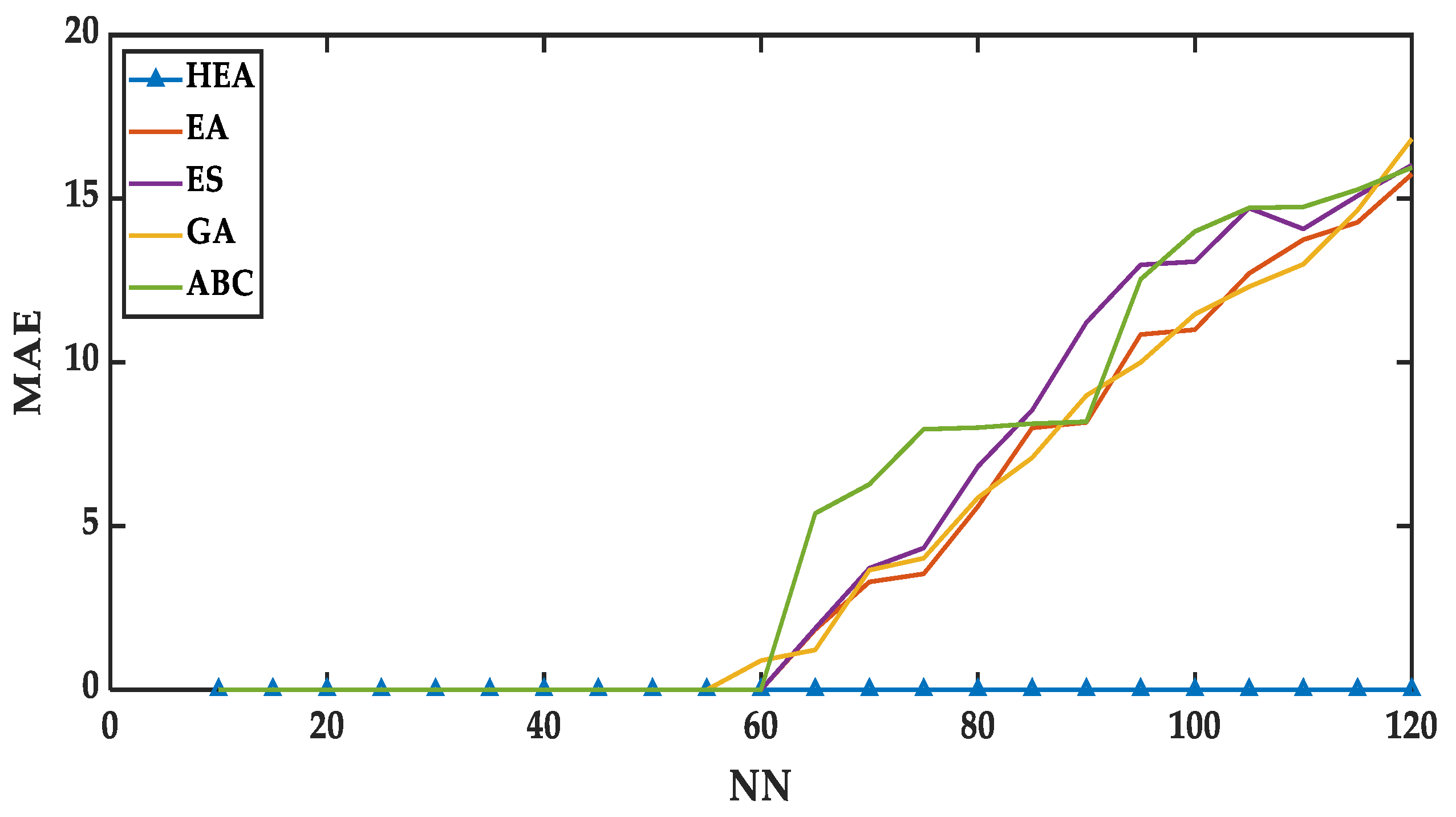
8.2. Testing Phase

The error analysis in the testing phase is sketched in Figure 7 and

Table 7. Tabulated MAE-Testing values for different DHNN-RANkSAT models.

NN	HEA	EA	ES	GA	ABC
10	0	0	0	0	0
15	0	0	0	0	0
20	0	0	0	0	0
25	0	0	0	0	0
30	0	0	0	0	0
35	0	0	0	0	0
40	0	0	0	0	0
45	0	0	0	0	0
50	0	0	0	0	0
55	0	0	11	40	0
60	0	0	20	60	0
65	0	0	30	80	0
70	0	0	40	80	0
75	0	40	60	100	0
80	0	60	60	100	0
85	0	60	60	100	15
90	0	80	80	100	20
95	0	80	100	100	30
100	0	80	100	100	40
105	0	80	100	100	40
110	0	80	100	100	60
115	0	80	100	100	65
120	0	80	100	100	70
AVG	0	31.304	41.782	54.783	14.782
MIN	0	0	0	0	0
MAX	0	80	100	100	70
AVG. RANK	2	2.89	3.67	4.09	2.56

. In this section, the behavior of various models in terms of synaptic weight management that retrieve the final states of neurons and produce global minima solutions are discussed. The competence of the testing phase in DHNN will be the indicator of ${\alpha }_{\mathrm{RAN}3\mathrm{SAT}}^k$ model which can successfully achieve optimal synaptic weights to retrieve the final states that produce global minima solutions.

Referring to Figure 7,${\alpha }_{\mathrm{RAN}k\mathrm{SAT}}^{ES}$ generates zero MAE value with lower $NN$ whereas the testing-MAE value sharply rises and reaches maximum error that is $MAE=100$ when $NN$ is higher. This has happened due to ${\alpha }_{\mathrm{RAN}k\mathrm{SAT}}^{ES}$ generating the wrong synaptic weight for higher $NN$, which complies with the sub-optimal training phase. However, the models ${\alpha }_{\mathrm{RAN}k\mathrm{SAT}}^{EA},{\alpha }_{\mathrm{RAN}k\mathrm{SAT}}^{GA},{\alpha }_{\mathrm{RAN}k\mathrm{SAT}}^{ABC}$ also failed to achieve its desired correct synaptic weight for higher $NN$, and this creates a higher testing-MAE value. This happened due to more $NN$, ${\alpha }_{\mathrm{RAN}k\mathrm{SAT}}^{EA},{\alpha }_{\mathrm{RAN}k\mathrm{SAT}}^{GA},{\alpha }_{\mathrm{RAN}k\mathrm{SAT}}^{ABC}$, which cannot explore the search space properly, which affects minimizing the cost function. To avoid this issue in the future, these models can adopt a greedy selection operator that can avoid sub-optimal solutions [48].

On the other hand, we can investigate the scenario of ${\alpha }_{\mathrm{RAN}k\mathrm{SAT}}^{HEA}$, which depicts the best performance in the testing phase. From the initial stage to $NN=120$, the proposed ${\alpha }_{\mathrm{RAN}k\mathrm{SAT}}^{HEA}$ creates the finest result achieving almost zero MAE values in the testing phase. This has happened since ${\alpha }_{\mathrm{RAN}k\mathrm{SAT}}^{HEA}$ has two filtering phases (fitness and diversity) are mentioned in the multi-objective concepts, which have several layers. These layers have a strategy for improving global search space, which is an exploration and local search space, which is known as exploitation. This strategy generates a zero-value cost function for ${\alpha }_{\mathrm{RAN}k\mathrm{SAT}}^{HEA}$ that leads to 100% global minimum solutions. Importantly, if the mechanism of ${\alpha }_{\mathrm{RAN}k\mathrm{SAT}}^{HEA}$ failed to retrieve optimal synaptic weight, the testing phase will be affected. Hence, it can be validated that ${\alpha }_{\mathrm{RAN}k\mathrm{SAT}}^{HEA}$ is a better model for finding global minima solutions compared to the other mentioned models.

Here, the Friedman test is conducted in Table 7 for ${\alpha }_{\mathrm{RAN}k\mathrm{SAT}}^{EA}{\alpha }_{\mathrm{RAN}k\mathrm{SAT}}^{ES},{\alpha }_{\mathrm{RAN}k\mathrm{SAT}}^{GA},{\alpha }_{\mathrm{RAN}k\mathrm{SAT}}^{ABC}$ and ${\alpha }_{\mathrm{RAN}k\mathrm{SAT}}^{HEA}$ models. The degree of freedom is $df=4$, considering $a_0=0.05$, and the Chi-Square value for the MAE-fitness is ${\chi }^2=51.399$. The null hypothesis of equal performance for all the models is rejected. Furthermore, the lowest value of an average rank represents the better position of a model. Here, we also check the rank analysis of the models through Table 7 and identify that the lowest rank occurred for ${\alpha }_{\mathrm{RAN}k\mathrm{SAT}}^{HEA}$ model, which is 2.00.

Energy Analysis

In this section, the types of energy analysis for different DHNN models are explained. Here, Figure 8 and

Table 8. Tabulated values of RGS for different DHNN-RANkSAT models.

NN	HEA	EA	ES	GA	ABC
10	1	1	1	1	1
15	1	1	1	1	1
20	1	1	1	1	1
25	1	1	1	1	1
30	1	1	1	1	1
35	1	1	1	1	1
40	1	1	1	1	1
45	1	1	1	1	1
50	1	1	1	1	1
55	1	0.2	0.2	1	1
60	1	0.2	0.2	0.2	1
65	1	0.2	0.2	0.2	1
70	1	0.2	0.2	0.2	1
75	1	0.2	0.2	0.2	1
80	1	0.2	0.2	0.2	1
85	1	0.08	0.12	0.2	1
90	1	0.04	0.04	0.12	1
95	1	0.04	0	0.12	1
100	1	0.04	0	0.12	0.8
105	1	0.04	0	0.12	0.2
110	1	0.04	0	0.04	0.2
115	1	0.04	0	0.04	0
120	1	0.04	0	0.04	0
AVG	1	0.659	0.450	0.513	0.834
MIN	1	0.04	0	0.04	0
MAX	1	1	1	1	1
AVG. RANK	4	2.86	2.13	2.85	3.57

elucidate the ratio of global solutions $(RGS)$ reached by ${\alpha }_{\mathrm{RAN}k\mathrm{SAT}}^{ES},{\alpha }_{\mathrm{RAN}k\mathrm{SAT}}^{EA}$ and ${\alpha }_{\mathrm{RAN}k\mathrm{SAT}}^{HEA}$ models. Figure 9 and

Table 9. Tabulated MAE-Energy values for different DHNN-RANkSAT models.

NN	HEA	EA	ES	GA	ABC
10	0	0	0	0	0
15	0	0	0	0	0
20	0	0	0	0	0
25	0	0	0	0	0
30	0	0	0	0	0
35	0	0	0	0	0
40	0	0	0	0	0
45	0	0	0	0	0
50	0	0	0	0	0
55	0	0	0	0	0
60	0	0	0	0.895	0
65	0	1.839	1.88	1.221	5.39
70	0	3.298	3.717	3.657	6.28
75	0	3.543	4.333	4.02	7.96
80	0	5.601	6.821	5.871	8.01
85	0	8.003	8.541	7.09	8.13
90	0	8.169	11.222	8.991	8.19
95	0	10.854	12.982	10	12.54
100	0	11	13.079	11.473	14
105	0	12.72	14.714	12.314	14.72
110	0	13.75	14.077	13	14.75
115	0	14.28	15.089	14.65	15.28
120	0	15.75	16.029	16.826	15.95
AVG	0	4.731	5.325	4.783	5.704
MIN	0	0	0	0	0
MAX	0	15.75	16.029	16.826	15.95
AVG.RANK	1.93	2.67	3.63	3.00	3.76

represent the difference in energy examined by measuring the MAE value with different $NN$.

In Figure 8 and Table 8, we can check whether the number of negative literals of 3SAT and 2SAT clauses influences the $RGS$. The capability of a model in achieving $RGS=1$, indicates the effectiveness of a proposed model to produce a consistent final neuron state. In this figure, we see that ${\alpha }_{\mathrm{RAN}k\mathrm{SAT}}^{ES},{\alpha }_{\mathrm{RAN}k\mathrm{SAT}}^{EA},{\alpha }_{\mathrm{RAN}k\mathrm{SAT}}^{GA}$ approaches $RGS\to 1$ for a certain interval $10\le NN\le 60$. Conversely, this consistency is degraded when $NN$ increases. At $NN\ge 60$ the $RGS$ for ${\alpha }_{\mathrm{RAN}k\mathrm{SAT}}^{ABC},{\alpha }_{\mathrm{RAN}k\mathrm{SAT}}^{EA},{\alpha }_{\mathrm{RAN}k\mathrm{SAT}}^{GA}$ has rapidly drops, and for $NN\ge 100$, it approaches zero. This is happened due to the presence of more 2SAT clauses, which creates more non-satisfied interpretations as well as no logical variety involved to overcome the final neuron states effectively. Though ${\alpha }_{\mathrm{RAN}k\mathrm{SAT}}^{ABC},{\alpha }_{\mathrm{RAN}k\mathrm{SAT}}^{EA}$ have a good optimizer, there are no specific objectives that can improve the logical rule and the operators cannot explore and exploit it properly.

Interestingly, our proposed ${\alpha }_{\mathrm{RAN}k\mathrm{SAT}}^{HEA}$ consistently produces the highest ratio of global solutions in the interval $10\le NN\le 120$. The abovementioned optimal range consistently produces $RGS=1$ for ${\alpha }_{\mathrm{RAN}k\mathrm{SAT}}^{HEA}$. This is caused since ${\alpha }_{\mathrm{RAN}k\mathrm{SAT}}^{HEA}$ employs the multi-objective function concept, which brings a different number of solutions by introducing negative states in the diversity phase of 3SAT and 2SAT clauses. More importantly, the appropriate placement of the local and global search operators tends $RGS=1$. This logical variety includes the ideal neuron state where the HTAF update the final neuron state successfully.

In the ${\alpha }_{\mathrm{RAN}k\mathrm{SAT}}^{HEA}$ mechanism, both exploration (negative and coalition campaign) and exploitation (positive and caretaker party) function equally for which this ${\alpha }_{\mathrm{RAN}k\mathrm{SAT}}^{HEA}$ executes only a single iteration in comparison to other models. Hence, the $RGS$ obtained by the ${\alpha }_{\mathrm{RAN}k\mathrm{SAT}}^{HEA}$ model has a good agreement of the work by [15] where $RGS$ approaching 1 can achieve 100% global minimum energy.

Here, the Friedman test results for ${\alpha }_{\mathrm{RAN}k\mathrm{SAT}}^{EA}{\alpha }_{\mathrm{RAN}k\mathrm{SAT}}^{ES},{\alpha }_{\mathrm{RAN}k\mathrm{SAT}}^{GA},{\alpha }_{\mathrm{RAN}k\mathrm{SAT}}^{ABC}$ and ${\alpha }_{\mathrm{RAN}k\mathrm{SAT}}^{HEA}$ models have been demonstrated in the Table 8. The degree of freedom is $df=4$, considering $a_0=0.05$, and the Chi-Square value for $RGS$ is ${\chi }^2=42.041$. The null hypothesis of equal performance for all the models is rejected. Furthermore, the higher $RGS$ value of an average rank represents the better position of a model. Here, we also check the rank analysis of the models through Table 8 and identify that the highest value for $RGS$ occurred for ${\alpha }_{\mathrm{RAN}k\mathrm{SAT}}^{HEA}$ model, which is 4.00.

In terms of energy analysis, Figure 9 and Table 9 illustrate how the MAE value between the minimum energy ($H_{{\alpha }_{\mathrm{RAN}3\mathrm{SAT}}^k}^{min}$) and final energy ($H_{{\alpha }_{\mathrm{RAN}3\mathrm{SAT}}^k}$) is used to examine the difference in energy. From the mentioned Figure and Table, we also observe a similar trend for ${\alpha }_{\mathrm{RAN}k\mathrm{SAT}}^{ES},{\alpha }_{\mathrm{RAN}k\mathrm{SAT}}^{EA},{\alpha }_{\mathrm{RAN}k\mathrm{SAT}}^{GA},{\alpha }_{\mathrm{RAN}k\mathrm{SAT}}^{ABC}$ models in which the MAE value in the energy analysis is sharply increasing in the interval of $60\le NN\le 120$. This takes place since ${\alpha }_{\mathrm{RAN}k\mathrm{SAT}}^{ES},{\alpha }_{\mathrm{RAN}k\mathrm{SAT}}^{EA},{\alpha }_{\mathrm{RAN}k\mathrm{SAT}}^{GA},{\alpha }_{\mathrm{RAN}k\mathrm{SAT}}^{ABC}$ cannot generate more satisfied solution strings for which it requires higher iterations that are trapped to local optima. On the other hand, our proposed ${\alpha }_{\mathrm{RAN}k\mathrm{SAT}}^{HEA}$ model has no error that is zero MAE value from the initial point until the end of the simulation. This has happened due to the generating satisfied solution strings following Equations (18) and (19). After the mutation the caretaker party ${\alpha }_{\mathrm{RAN}k\mathrm{SAT}}^{HEA}$ has a large capacity in achieving more satisfied solution strings, which arises zero MAE value for energy analysis and satisfied Equation (16) with tolerance value accurately. Despite creating intelligence effort throughout the learning phase, this network has been presented with an excellent error reduction mechanism to prevent non-improving solutions. As a result, the neuron state for ${\alpha }_{\mathrm{RAN}k\mathrm{SAT}}^{HEA}$ has minimum state oscillation and has been updated properly during the testing phase.

In Table 9, the Friedman test directed for ${\alpha }_{\mathrm{RAN}k\mathrm{SAT}}^{EA}{\alpha }_{\mathrm{RAN}k\mathrm{SAT}}^{ES},{\alpha }_{\mathrm{RAN}k\mathrm{SAT}}^{GA},{\alpha }_{\mathrm{RAN}k\mathrm{SAT}}^{ABC}$ and ${\alpha }_{\mathrm{RAN}k\mathrm{SAT}}^{HEA}$ models. The degree of freedom is $df=4$, considering $a_0=0.05$, and the Chi-Square value for Energy-MAE is ${\chi }^2=37.536$. The null hypothesis of equal performance for all the models is rejected. Furthermore, the lower value of an average rank represents the better position of a model. Here, we also check the rank analysis of the models through Table 9 and recognize that the lowest rank value for MAE-Energy occurred for the ${\alpha }_{\mathrm{RAN}k\mathrm{SAT}}^{HEA}$ model, which is 1.93.

8.3. Similarity Index

In Figure 10 and Figure 11 as well as

Table 10. Tabulated $TNV$ values for different DHNN-RANkSAT models.

NN	HEA	EA	ES	GA	ABC
10	21.4	17.8	15.4	6.2	13
15	36	35	38.8	33	22
20	68.4	36.6	55	46.2	31
25	78.8	75	69.4	56.6	72
30	90.2	77.2	77	64.2	81
35	96	76.5	81.8	73.6	82.8
40	96.4	90.8	87.4	81	81.6
45	98.6	95	93	85	94
50	99	98.6	94.8	91.8	92
55	99.2	92.8	90	69.2	95
60	99.4	93	78.8	48	100
65	100	57	59	44.2	80.5
70	100	47.4	49	39	55
75	100	39.8	39	32	35
80	100	40	48	23	25
85	100	40	40	20.5	20
90	100	20	12.8	13	20
95	100	20	0	12.5	20
100	100	20	0	12.5	20
105	100	20	0	0	20
110	100	20	0	0	0
115	100	20	0	0	0
120	100	20	0	0	0
AVG	90.583	50.108	44.747	37.053	46.083
MIN	21.4	17.8	0	0	0
MAX	100	98.6	94.8	91.8	100
AVG. RANK	4.91	3.33	2.52	1.46	2.78

and

Table 11. Tabulated GLI values for different DHNN-RANkSAT models. The notation * means no value has been generated in that particular point.

NN	HEA	EA	ES	GA	ABC
10	0.676	0.624	0.603	0.711	0.671
15	0.668	0.619	0.680	0.698	0.698
20	0.694	0.687	0.677	0.724	0.667
25	0.724	0.687	0.692	0.703	0.704
30	0.730	0.695	0.698	0.744	0.704
35	0.705	0.728	0.701	0.731	0.697
40	0.729	0.739	0.715	0.758	0.724
45	0.721	0.724	0.709	0.838	0.728
50	0.750	0.738	0.746	0.812	0.719
55	0.719	0.710	0.734	0.793	0.666
60	0.763	0.706	0.709	0.590	0.619
65	0.777	0.579	0.677	0.551	0.606
70	0.742	0.497	0.469	0.490	0.559
75	0.731	0.316	0.271	0.387	0.487
80	0.760	0.311	0.291	0.298	0.341
85	0.749	0.304	0.244	0.224	0.311
90	0.751	0.154	0.257	0.198	0.324
95	0.749	0.167	*	*	0.134
100	0.760	0.146	*	*	0.145
105	0.770	0.151	*	*	0.126
110	0.748	0.159	*	*	*
115	0.751	0.156	*	*	*
120	0.749	0.159	*	*	*
AVG	0.735	0.466	0.429	0.446	0.459
MIN	0.668	0.146	0.257	0.198	0.126
MAX	0.777	0.739	0.746	0.838	0.728
AVG. RANK	1.87	1.59	1.17	1.67	1.64

, we have examined the similarity and dissimilarity of the obtained final neuron states using the similarity index (SI). This indexing is specific for binary variables and use for divergency studies [49]. In the similarity index analysis, we have looked for the study of Total Neuron Variation (TNV) and the Gower–Legendre Index (GLI) according to the Equations (40) and (39).

8.3.1. Total Neuron Variation ($TNV$)

Figure 10 and Table 10 show the evaluation of total neuron variation ($TNV$) for various DHNN-RANkSAT models. The performance of ${\alpha }_{\mathrm{RAN}k\mathrm{SAT}}^{ES},{\alpha }_{\mathrm{RAN}k\mathrm{SAT}}^{EA},{\alpha }_{\mathrm{RAN}k\mathrm{SAT}}^{GA},{\alpha }_{\mathrm{RAN}k\mathrm{SAT}}^{ABC}$ and ${\alpha }_{\mathrm{RAN}k\mathrm{SAT}}^{HEA}$ with DHNN in terms of variation of final neuron states in the training phase will be examined in this section. According to the finding, the neuron variations generate for ${\alpha }_{\mathrm{RAN}k\mathrm{SAT}}^{ES},{\alpha }_{\mathrm{RAN}k\mathrm{SAT}}^{EA},{\alpha }_{\mathrm{RAN}k\mathrm{SAT}}^{GA}$ are slowly growing up, and these models have achieved maximum peak with $TNV=94.8,TNV=98.6$ and $TNV=91.8$, respectively in $NN=50$. The model ${\alpha }_{\mathrm{RAN}k\mathrm{SAT}}^{ABC}$ reached the highest peak at $NN=60$ and achieved $TNV=100$.

After $NN=50$ and $NN=60$, the number of solution variations for the ${\alpha }_{\mathrm{RAN}k\mathrm{SAT}}^{ES},{\alpha }_{\mathrm{RAN}k\mathrm{SAT}}^{EA},{\alpha }_{\mathrm{RAN}k\mathrm{SAT}}^{GA},{\alpha }_{\mathrm{RAN}k\mathrm{SAT}}^{ABC}$ models continuously drops down, and after $NN\ge 100$, the neuron variation is very low for ${\alpha }_{\mathrm{RAN}k\mathrm{SAT}}^{EA}$ and almost zero for ${\alpha }_{\mathrm{RAN}k\mathrm{SAT}}^{ES},{\alpha }_{\mathrm{RAN}k\mathrm{SAT}}^{GA},{\alpha }_{\mathrm{RAN}k\mathrm{SAT}}^{ABC}$. This is due to ${\alpha }_{\mathrm{RAN}k\mathrm{SAT}}^{ES}$ having no optimization layer that cannot explore the search space. A higher number of neurons ($NN$), ${\alpha }_{\mathrm{RAN}k\mathrm{SAT}}^{EA},{\alpha }_{\mathrm{RAN}k\mathrm{SAT}}^{GA},{\alpha }_{\mathrm{RAN}k\mathrm{SAT}}^{ABC}$ becomes stuck at local optima due to the inability of the key operators, such as advertising campaigns for EA in searching for solution space.

To the contrary, our proposed ${\alpha }_{\mathrm{RAN}k\mathrm{SAT}}^{HEA}$ model has gradually reached the peak and remained until the end of the simulation. This is owing to the efficient synaptic weight management and training provided by ${\alpha }_{\mathrm{RAN}k\mathrm{SAT}}^{HEA}$. Furthermore, ${\alpha }_{\mathrm{RAN}k\mathrm{SAT}}^{HEA}$ has two phases with four-layer optimization, which allows for the intensification and diversification of a large search space with the use of optimization operators. This model has manifested that the proposed logical structure is very effective in creating more variation of solutions as the number of neurons increases. Moreover, the variation analysis by ${\alpha }_{\mathrm{RAN}k\mathrm{SAT}}^{HEA}$ shows the diversified negative literals impact of DHNN on the production of global solutions. Consequently, we can say that lower energy analysis (ratio global) affects the low performance $TNV$ (for ${\alpha }_{\mathrm{RAN}k\mathrm{SAT}}^{ES},{\alpha }_{\mathrm{RAN}k\mathrm{SAT}}^{EA},{\alpha }_{\mathrm{RAN}k\mathrm{SAT}}^{GA},{\alpha }_{\mathrm{RAN}k\mathrm{SAT}}^{ABC}$) and higher energy analysis (ratio global) depicts the increased performance of $TNV$ for ${\alpha }_{\mathrm{RAN}k\mathrm{SAT}}^{HEA}$.

In Table 10, the Friedman test directed for ${\alpha }_{\mathrm{RAN}k\mathrm{SAT}}^{EA}{\alpha }_{\mathrm{RAN}k\mathrm{SAT}}^{ES},{\alpha }_{\mathrm{RAN}k\mathrm{SAT}}^{GA},{\alpha }_{\mathrm{RAN}k\mathrm{SAT}}^{ABC}$ and ${\alpha }_{\mathrm{RAN}k\mathrm{SAT}}^{HEA}$ models. The degree of freedom is $df=4$, considering $a_0=0.05$, and the Chi-Square value for $TNV$ is ${\chi }^2=61.511$. The null hypothesis of equal performance for all the models is rejected. Furthermore, the highest value of an average rank represents the best position of a model. Here, we have also checked the rank analysis of the models through Table 10 and identified that the highest rank for $TNV$ has occurred for ${\alpha }_{\mathrm{RAN}k\mathrm{SAT}}^{HEA}$ model, which is 4.91.

8.3.2. Gower–Legendre Index (GLI)

Figure 11 and Table 11 portrayed the GLI value attained by different DHNN-RANkSAT models. GLI measures the similarity of negative states concerning the benchmark state. For this case, the higher GLI value is better for investigating the similarity index. In our analysis, the ${\alpha }_{\mathrm{RAN}k\mathrm{SAT}}^{ES},{\alpha }_{\mathrm{RAN}k\mathrm{SAT}}^{GA},{\alpha }_{\mathrm{RAN}k\mathrm{SAT}}^{ABC}$ models have recorded poor values 0.2, 0.198 and 0.126, respectively, for higher $NN$. This states that for higher $NN$, different number of negative states in the logical rule results valleys, which decrease to a lower value. Even at $95\le NN\le 120$, ${\alpha }_{\mathrm{RAN}k\mathrm{SAT}}^{ES},{\alpha }_{\mathrm{RAN}k\mathrm{SAT}}^{GA},{\alpha }_{\mathrm{RAN}k\mathrm{SAT}}^{ABC}$ cannot generate any value, which means that these models are trapped into 100% local minima solutions. Correspondingly, for higher $NN$, the GLI value is staked at 0.15, which is also very low. This ${\alpha }_{\mathrm{RAN}k\mathrm{SAT}}^{EA}$ model can generate a minimum GLI value at the end of the simulation because it can produce a few global solutions for higher $NN$ and the variables of each state for ${\alpha }_{\mathrm{RAN}3\mathrm{SAT}}^k$ obtained are not all equal to the ideal neuron states.

Nevertheless, the proposed ${\alpha }_{\mathrm{RAN}k\mathrm{SAT}}^{HEA}$ generates a designated value $0.65\le GLI\le 0.75$ until the end of the simulation, which shows a higher GLI value rather than other presented models. This demonstrates that the proposed ${\alpha }_{\mathrm{RAN}k\mathrm{SAT}}^{HEA}$ showcased with the different $NN$ do not affect the variation of final neuron states. Moreover, the composition of multi-objective concept effect ${\alpha }_{\mathrm{RAN}k\mathrm{SAT}}^{HEA}$ for higher GLI value since this proposed model makes a good alignment with RANkSAT representation. In addition, the higher GLI value admits the mechanism that is capable of finding ideal solution strings, which enhances the storage capacity of DHNN. This model successfully explored more diverse states that result in global minimum energy.

In Table 11, the Friedman test directed for ${\alpha }_{\mathrm{RAN}k\mathrm{SAT}}^{EA}{\alpha }_{\mathrm{RAN}k\mathrm{SAT}}^{ES},{\alpha }_{\mathrm{RAN}k\mathrm{SAT}}^{GA},{\alpha }_{\mathrm{RAN}k\mathrm{SAT}}^{ABC}$ and ${\alpha }_{\mathrm{RAN}k\mathrm{SAT}}^{HEA}$ models. The degree of freedom is $df=4$, considering $a_0=0.05$, and the Chi-Square value for GLI is ${\chi }^2=17.072$. The null hypothesis of equal performance for all the models is rejected. Furthermore, the highest value of an average rank represents the best position of a model. Here, we also check the rank analysis of the models through Table 11 and identify that the highest rank for GLI occurred for ${\alpha }_{\mathrm{RAN}k\mathrm{SAT}}^{HEA}$ model, which is 1.87.

From Figure 4, Figure 5, Figure 6, Figure 7, Figure 8, Figure 9, Figure 10 and Figure 11 and Table 5, Table 6, Table 7, Table 8, Table 9, Table 10 and Table 11, the scenario of the overall performances of the models is demonstrated. The final neuron states attained by the proposed ${\alpha }_{\mathrm{RAN}k\mathrm{SAT}}^{HEA}$ model is found very nominal in the over-fitting issue and obtain the highest neuron variation achieved at the end of the simulation. More importantly, the storage capability in terms of ideal solution strings, error calculations and energy analysis exposed that the ${\alpha }_{\mathrm{RAN}k\mathrm{SAT}}^{HEA}$ model achieved the highest global minima solutions, which correspond to global minimum energy. If we observe the compatibility of the mentioned models in terms of storage capacity, training analysis, testing analysis, energy analysis and similarity analysis our proposed DHNNRANkSAT-HEA model outperformed the traditional EA, ES, GA and ABC models.

8.4. Impact Analysis

The pioneer observation from the above discussions and analysis, it is clearly visible that ${\alpha }_{\mathrm{RAN}k\mathrm{SAT}}^{HEA}$ is superior to other presented models. The balanced exploration–exploitation mechanist, proper placement of the local–global search operators and the perfect intelligent mutation mechanism piled ${\alpha }_{\mathrm{RAN}k\mathrm{SAT}}^{HEA}$ as an unbeatable strength compared to other mentioned models with the optimal solutions. As shown in the pseudo-code of ${\alpha }_{\mathrm{RAN}k\mathrm{SAT}}^{HEA}$, the diversity phase was observed to explore more negative states that correspond to the projected solution string. For the exploration part, the trajectory of the fitness value is obtained by the ‘maximum fitness phase’ in the advertisement campaign (Negative advertisement and Coalition part).

This is contrary to other models (${\alpha }_{\mathrm{RAN}k\mathrm{SAT}}^{ES},{\alpha }_{\mathrm{RAN}k\mathrm{SAT}}^{EA},{\alpha }_{\mathrm{RAN}k\mathrm{SAT}}^{GA},{\alpha }_{\mathrm{RAN}k\mathrm{SAT}}^{ABC}$), which increase the gap between the desired outcome and the current fitness value of the population. In terms of exploitation, the Positive advertisement and Caretaker party of the advertisement campaign keep fasting to acquire the highest fitness value. The exploration and exploitation strategy assemble to achieve our objectives in a single iteration. On the other hand, other models do not acquire similar benefit because of unbalancing position of exploration–exploitation mechanisms that creates lower fitness value. Thus, ${\alpha }_{\mathrm{RAN}k\mathrm{SAT}}^{HEA}$ is reported to provide a positive impact although the initial population was initialized in random nature.

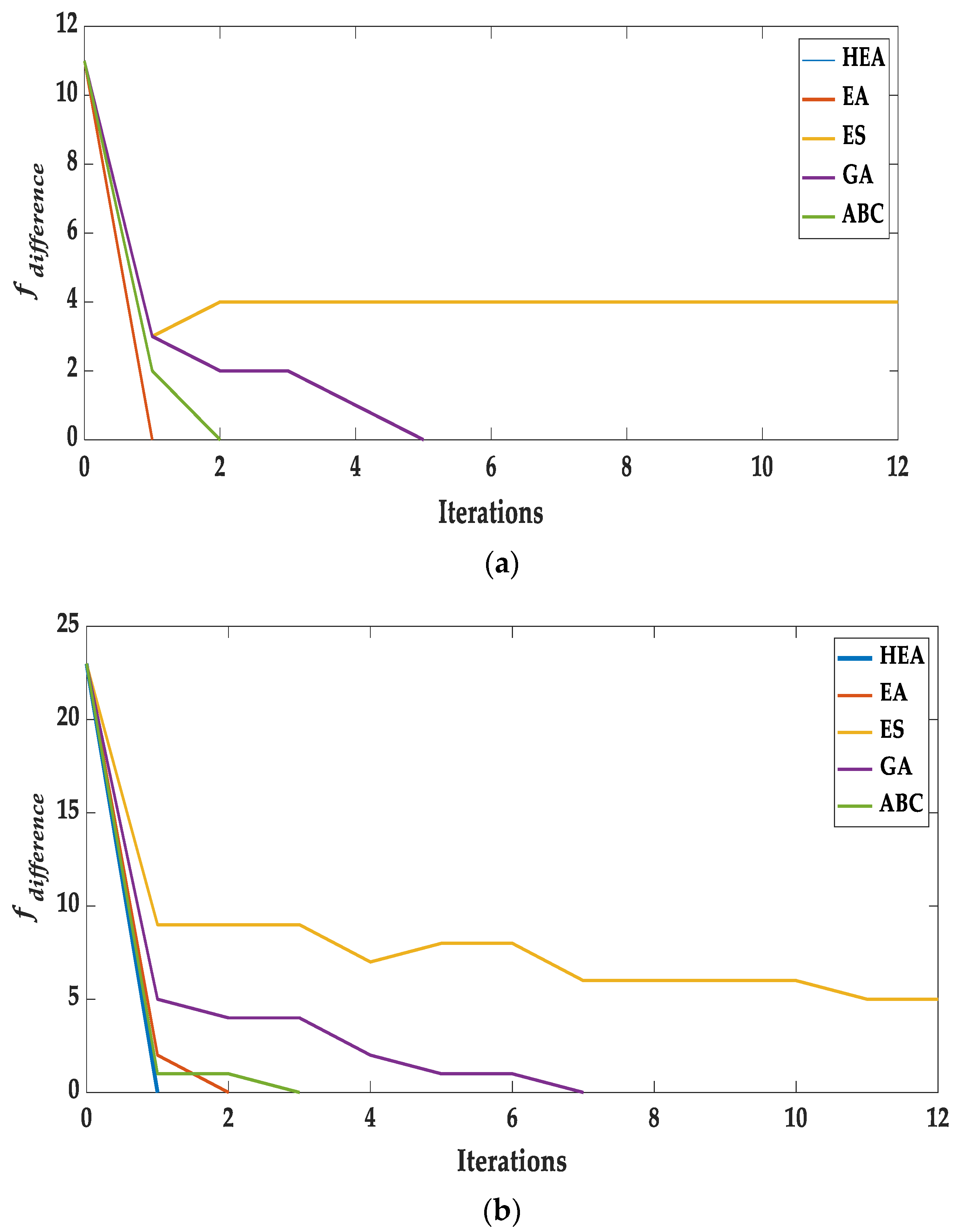
8.5. Convergence Analysis

In this experiment, Figure 12a–d shows the convergence behavior of the proposed ${\alpha }_{\mathrm{RAN}k\mathrm{SAT}}^{HEA}$ was compared with other state-of-the-art algorithms. The combined existence of the exploration and exploitation strategy of the proposed ${\alpha }_{\mathrm{RAN}k\mathrm{SAT}}^{HEA}$ is more balanced in comparison to other algorithms. As shown in Figure 12a–d, the convergence curve for different RANkSAT models illustrated that ${\alpha }_{\mathrm{RAN}k\mathrm{SAT}}^{HEA}$ requires only single iterations to obtain optimal solutions compared to other state-of-the-art algorithms. Having more exploitation mechanisms, the ${\alpha }_{\mathrm{RAN}k\mathrm{SAT}}^{HEA}$ model manages to avoid being trapped in the local solutions.

Although, ${\alpha }_{\mathrm{RAN}k\mathrm{SAT}}^{EA},{\alpha }_{\mathrm{RAN}k\mathrm{SAT}}^{ABC}$ showed competitive performances, the number of iterations requires more than the proposed model. Another obvious issue is that ${\alpha }_{\mathrm{RAN}k\mathrm{SAT}}^{GA}$ needs higher iterations since the operator is not quite effective. The models ${\alpha }_{\mathrm{RAN}k\mathrm{SAT}}^{EA},{\alpha }_{\mathrm{RAN}k\mathrm{SAT}}^{ABC}$ and ${\alpha }_{\mathrm{RAN}k\mathrm{SAT}}^{GA}$ have the primary weakness in terms of exploration and exploitation in deploying and utilizing the operators. This convergence analysis shows that ${\alpha }_{\mathrm{RAN}k\mathrm{SAT}}^{ES}$ failed to present the influence since it has no exploration and exploitations mechanisms.

8.6. Overall Comparative Overview of the Proposed ${\alpha }_{\mathrm{RAN}k\mathrm{SAT}}^{HEA}$ Method with Existing Methods

In this section, we consider a different number of neurons $(NN=30,60,90,120)$ to verify the effectiveness of the proposed model with some other standard models.

Table 12. Overall performance analysis for different DHNN-RANkSAT models.

Models	Fitness $\left({\mathit{f}}_{{\mathit{L}}_{\mathit{j}}}\right)$	$\mathbf{Diversity} ({\mathit{\nu }}_{\mathit{T}})$	MAE-Testing	$\mathbf{Number} \mathbf{of} \mathbf{Global} \mathbf{Solutions} ({\mathit{N}}_{\mathit{G}\mathit{l}\mathit{o}\mathit{b}\mathit{a}\mathit{l}})$	MAE-Energy	$\mathbf{Total} \mathbf{Neuron} \mathbf{Variations} (\mathit{T}\mathit{N}\mathit{V})$	Gower–Legendre Index (GLI)
${\alpha }_{RANkSAT}^{HEA}$	97.60%	98.08%	0	100%	0	97.40	74.82%
${\alpha }_{\mathrm{RAN}k\mathrm{SAT}}^{EA}$(Original version) [23]	80.31%	92.55%	40	70%	5.98	52.55	42.85%
${\alpha }_{\mathrm{RAN}k\mathrm{SAT}}^{ES}$ [12]	70.38%	89.07%	50	51%	6.81	42.15	41.6%
${\alpha }_{\mathrm{RAN}k\mathrm{SAT}}^{\begin{array}{l}\\ GA\end{array}}$ [19]	74.75%	91.30%	47.5	56%	6.68	38.80	38.30%
${\alpha }_{\mathrm{RAN}k\mathrm{SAT}}^{ABC}$ [45]	78.15%	92.73%	22.5	75%	6.04	50.25	41.17%

illustrates an overall comparison of ${\alpha }_{\mathrm{RAN}k\mathrm{SAT}}^{HEA}$ with existing methods with different metrics.

Based on Table 12, for different numbers of neurons ${\alpha }_{\mathrm{RAN}k\mathrm{SAT}}^{HEA}$ generated the superior result in terms of fitness accuracy, diversity accuracy, testing error, energy error, total neuron variations and similarity index analysis compared to other mentioned models. It means that ${\alpha }_{\mathrm{RAN}k\mathrm{SAT}}^{HEA}$ satisfies our desired objectives: maximum fitness value and diversified logical structure with desired ideal solution string that enhances the storage capacity of DHNN. It is worthwhile to discuss the intriguing fact revealed by the retrieval capability of DHNN in ensuring the final states of the neurons that lead to global convergence. The robust operators of the proposed ${\alpha }_{\mathrm{RAN}k\mathrm{SAT}}^{HEA}$ enhanced the capability of achieving the highest number of global solutions. In a nutshell, we can express that our proposed ${\alpha }_{\mathrm{RAN}k\mathrm{SAT}}^{HEA}$ model outperformed all the mentioned models.

8.7. Pareto Optimality Analysis

The performance of ${\alpha }_{\mathrm{RAN}k\mathrm{SAT}}^{HEA}$ in doing multi-objective function can be examined through Pareto front solutions [50]. Here, Figure 13 explains the Pareto frontier of a multi-objective function with two criteria where most points belong to the Pareto frontier area. This figure delineates several important features—dominated states, non-dominated states, Pareto front and Ideal objective state of Pareto optimality for a multi-objective function.

Generally, the Pareto front consists of the set of best trade-off points, which are noted as the non-dominated points. While the Ideal states define the upper bounds (optimal points) for the objective function values, respectively. According to the study of [51], the neuron state produced by the ${\alpha }_{\mathrm{RAN}k\mathrm{SAT}}^{HEA}$ model as shown in Figure 14 that follows the non-dominated states as well as upper bound states which achieves Ideal states.

However, our proposed model does not entirely incorporate the concept of Pareto dominance in the selection of Ideal strings. Our proposed ${\alpha }_{\mathrm{RAN}k\mathrm{SAT}}^{HEA}$ relies greatly in the competency of both objective functions. In this context, an Ideal string must comply with maximum fitness with logical diversity that are stored in CAM (DHNN). When the string achieves maximum fitness then it proceeds to the diversity phase. The mechanism continues unless any one of the phases failed to satisfy the objective functions. Moreover, the Pareto optimality can be considered when five (5) ideal solution strings fail to generate in a simulation. In our total simulation $(10\le NN\le 120)$, the proposed model successfully achieved five ideal solution strings. Hence, the sub optimal neuron state for ${\alpha }_{\mathrm{RAN}k\mathrm{SAT}}^{HEA}$ cannot be found and analyzed.

9. Conclusions

This paper reveals a novel multi-objective DHNNRANkSAT-HEA model, and a new insight into the non-systematic logical rule for a high dimensional decision system. A higher order logical structure addressed as RANkSAT (for $k=3,2$) is formed to optimize the cost function of DHNN. This paper proposed a novel multi-objective function that capitalize maximum fitness and diversified ratio of negative literals in each clause with five ideal solution strings that increase the storage capacity of DHNN.

A new hybrid metaheuristic, named Hybrid Election Algorithm (HEA), is also proposed by introducing a dynamic ‘Caretaker party’ operator in the mechanism of an advertisement campaign that improves the quality of local solutions. More importantly, our proposed model is capable of maintaining balance between the exploration–exploitation strategy for which it can avoid sub optimal solutions. Importantly, our proposed DHNNRANkSAT-HEA model successfully interprets to minimize the cost function within a single iteration during the training phase. Finally, we observed from the experimental evaluations and statistical and impact analysis that our proposed DHNNRANkSAT-HEA model achieved superior results in comparison with other models.

According to the famous no-free-lunch theorem [52], no metaheuristic/algorithm can perform equally well in all types of conditions. In this regard, our model might not guarantee that it can be successfully implemented on other ANNs, such as the Radial Basis Function Neural Network, since each ANN model has individual architecture analysis. On the other hand, this DHNNRANkSAT-HEA model has several shortcomings that could be addressed in future research. We emphasize that our proposed model limits the number of maximum combinations (COMBMAX), which also limits the simulation ability to generate satisfiable neuron states. Furthermore, this study stops at 120 neurons, in contrast to [23], which takes up to 300 neurons. This discussion also verified that the compatibility of ${\alpha }_{\mathrm{RAN}k\mathrm{SAT}}^{3,2}$ with the proposed ${\alpha }_{\mathrm{RAN}k\mathrm{SAT}}^{HEA}$ model in DHNN logic programming can be applied in the logic/data mining field [53,54] in the next exploration.