Calculation of Critical Load of Axially Functionally Graded and Variable Cross-Section Timoshenko Beams by Using Interpolating Matrix Method

Abstract

In this paper, the interpolation matrix method (IMM) is proposed to solve the buckling critical load of axially functionally graded (FG) Timoshenko beams. Based on Timoshenko beam theory, a set of governing equations coupled by the deflection function and rotation function of the beam are obtained. Then, the deflection function and rotation function are decoupled and transformed into an eigenvalue problem of a variable coefficient fourth-order ordinary differential equation with unknown deflection function. According to the theory of interpolation matrix method, the eigenvalue problem of the variable coefficient fourth-order ordinary differential equation is transformed into an eigenvalue problem of a set of linear algebraic equations, and the critical buckling load and the corresponding deflection function of the axially functionally graded Timoshenko beam can be calculated by the orthogonal triangular (QR) decomposition method, which is the most effective and widely used method for finding all eigenvalues of a matrix. The numerical results are in good agreement with the existing results, which shows the effectiveness and accuracy of the method.

1. Introduction

The performance of functionally graded (FG) material varies continuously in a certain direction in space to meet the needs of a variety of special engineering structures, with the advantage that there is no significant interface between the two-phase materials, avoiding the stress concentration that occurs when the material is heated or cooled [1]. Reviewing the literature on FG materials, it is understood that the literature is mostly dedicated to the analysis of plates and shells made of FG materials and relatively few research works have been carried out on FG beams. Moreover, most of the research works on FG beams are devoted to certain types of FG beams with material properties of varying thicknesses; very few studies exist on FG beams with material gradation along the beam axis.

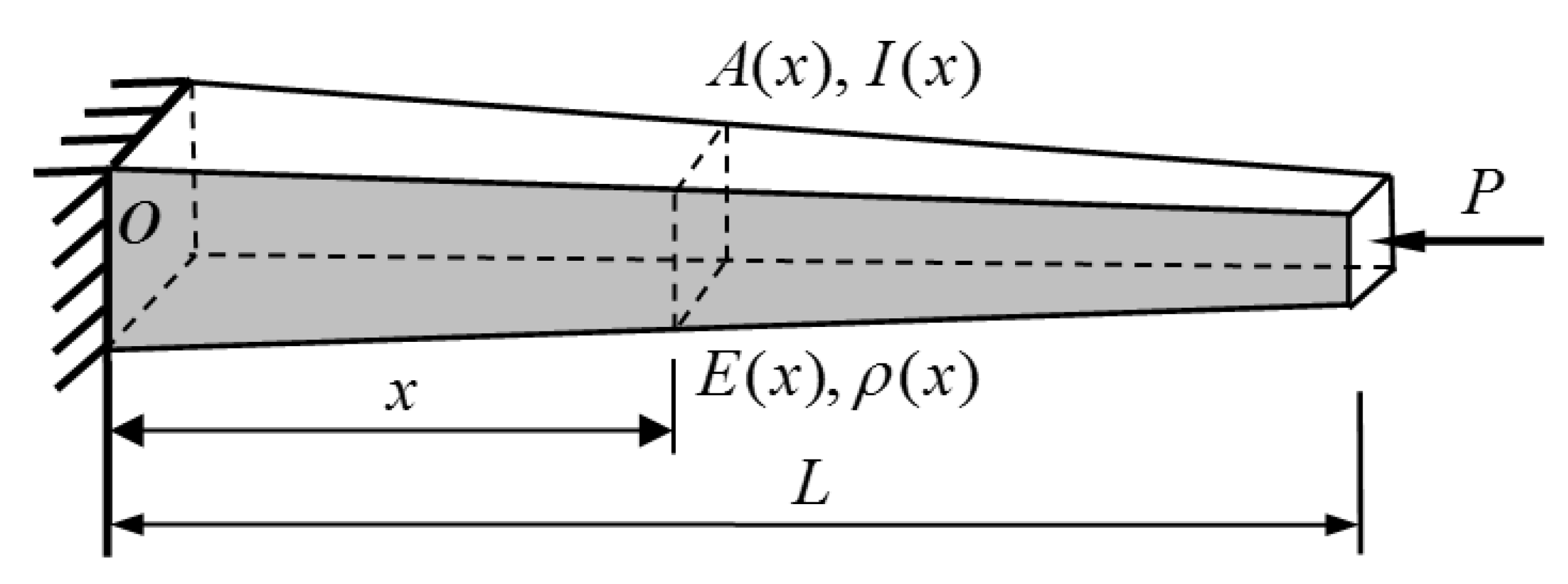
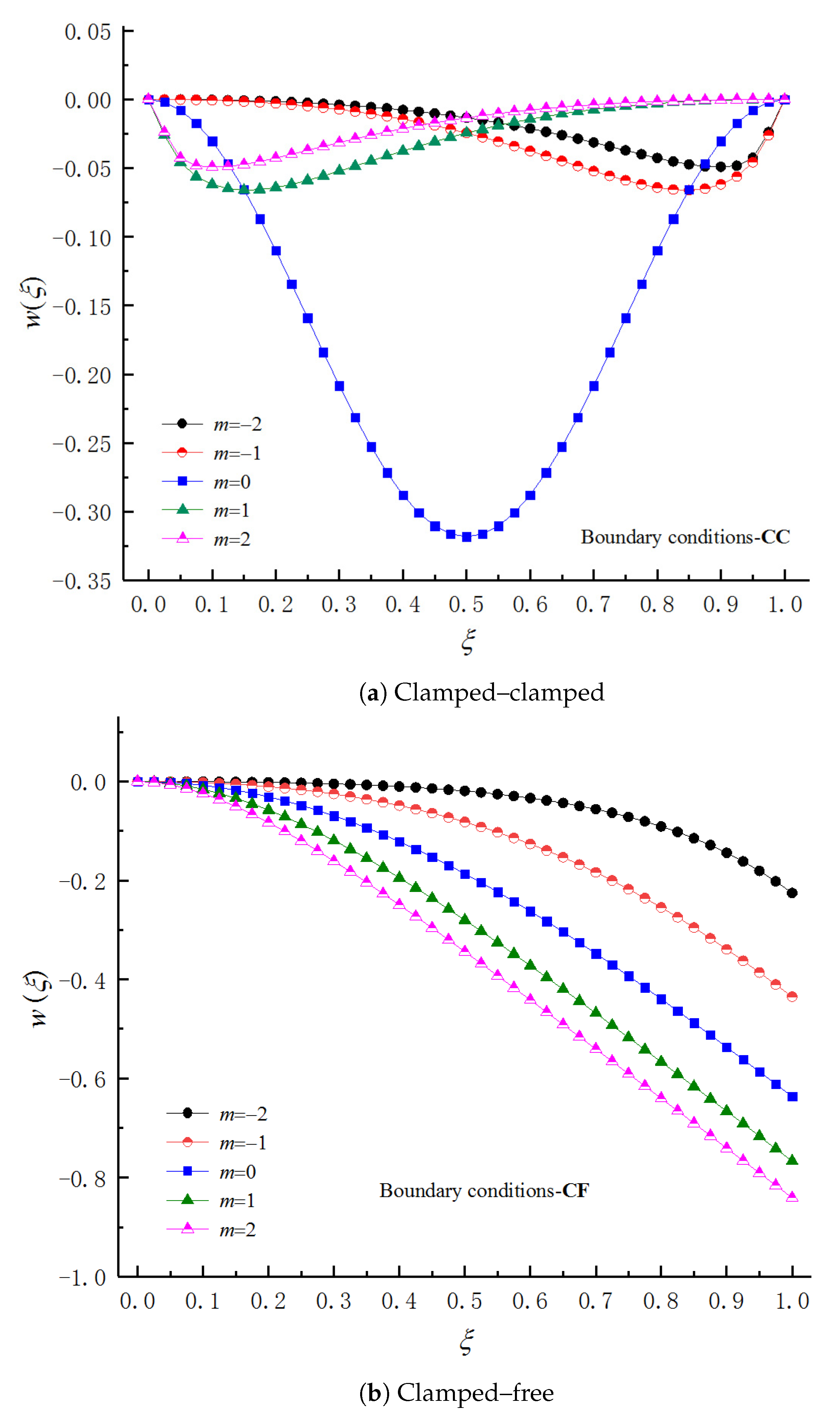
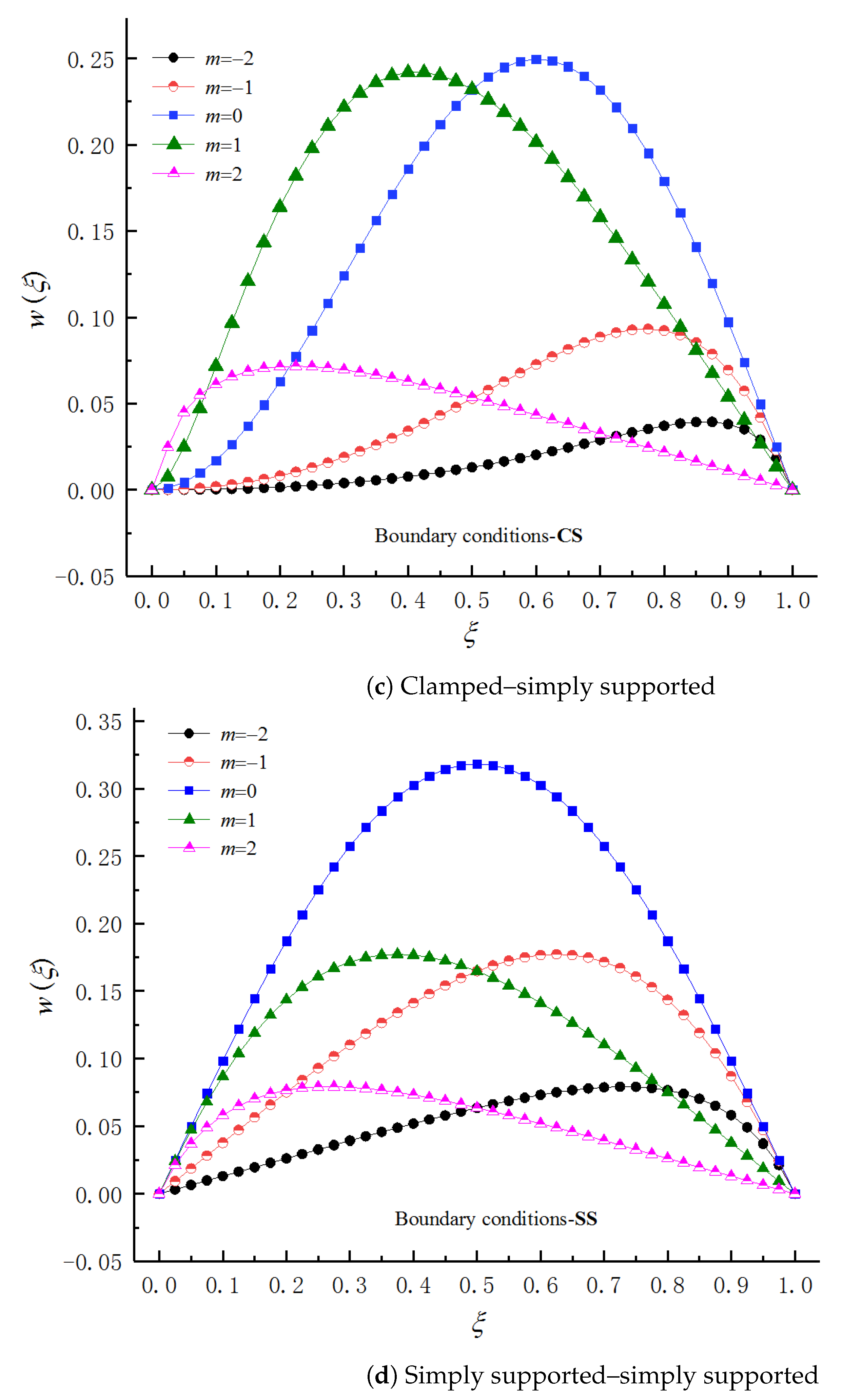
In order to simplify the problem, the Euler–Bernoulli beam model is generally used to discuss the buckling problem of an axially functionally graded beam with a variable cross-section in engineering study of the buckling critical load of beam structural elements. Since the theory neglects the effect of rotation and shear deformation of beam section, the calculated values of critical load are significantly higher than the actual results; therefore, Euler–Bernoulli beam theory is only applicable to slender beams. Shahba et al. [2] solved the governing differential equations of the free vibration and buckling of axial functionally graded variable-section Euler–Bernoulli beams by using two numerical methods: the differential transformation element method (DTEM) and the lowest-order differential quadrature element method (DQEL). Based on Euler–Bernoulli theory, Elishakoff et al. [3,4] obtained the exact solution of the critical buckling load of non-uniform beams by using an inverse method and a semi-inverse method, but this method cannot solve the problems under all boundary conditions. Shahba et al. [5,6] propose a new beam element which uses the shape function of a homogeneous beam element and the finite element method to analyze the free vibration and buckling of axially functionally graded tapered Euler–Bernoulli beam. Timoshenko beam theory considers shear deformation and moment of inertia, so the theory gives a more accurate model. However, the solution of the buckling of beams based on Timoshenko beam theory will face difficulties in solving mathematical problems, mainly because the control equation obtained by Timoshenko beam theory is a variable coefficient differential equation coupled by deflection and rotation, and it is quite difficult to find the analytical solution of the critical load of axially functionally graded Timoshenko beams with variable cross-sections. Therefore, approximate and numerical methods are generally used to solve the dynamic problem of axial heterogeneous Timoshenko beams. Tong et al. [7] studied the free vibration of Timoshenko beams by using the stepwise reduction method. Zhou et al. [8] studied the free vibration of Timoshenko beams by using Rayleigh’s law. Ozgumus et al. [9] used the differential transformation method to solve the differential equation of motion with variable coefficients, and analyzed the free vibration of Timoshenko beams. Shahba A. et al. [10] used the finite element method to study the effects of taper ratio, elastic constraints, added mass, and material heterogeneity on the critical buckling load of Timoshenko beams. Rajasekaran [11] combines the dynamic stiffness matrix method with the differential transformation method to study the critical buckling load of axially functionally graded Timoshenko beams with variable cross-sections. Yong et al. [12] introduced the auxiliary function of power series, transformed the characteristic differential equations of Timoshenko beams coupled with deflection and rotation into a set of linear algebraic characteristics, and solved the critical buckling load of the beam. Based on the improved Rayleigh’s law, De et al. [13] used Mathematica software to solve the free vibration and buckling problems of engineering structural elements. Bazeos et al. [14] used an approximate algorithm to quickly and effectively calculate the dimensionless buckling critical load of a tapered pile. Iremonger et al. [15] analyzed the buckling of a tapered pile and a stepped pile by using the finite difference method and the matrix iteration method. Rajasekaran et al. [16] studied the free vibration, buckling, and static bending of axially functionally graded nano-tapered Timoshenko and Bernoulli–Euler beams based on the nonlocal Timoshenko beam theory. Based on the nonlocal Timoshenko beam theory, Robinson et al. [17] studied the buckling critical load of axially functionally graded material Timoshenko beams with variable cross-sections. Deng et al. [18] established the exact dynamic stiffness matrix of an axial functionally graded material Timoshenko double-beam system on Winkler–Pasternak under an axial load, considered the damping effect of a connecting layer, and obtained the accurate buckling critical load through the Wittrick–Williams algorithm. Aydogdu [19] studied the free vibration and stability of axially graded simply supported beams by the semi-inverse method, which can be used to optimize the frequency and buckling loads of these FG beams. beams with variable cross sections under different boundary conditions. Yuan et al. [20] studied the free vibration and stability of Timoshenko and Euler–Bernoulli beams by using the exact dynamic stiffness method. In this paper, based on the motion control equation of axially functionally graded Timoshenko beams with variable cross sections derived from reference [10,11], a differential equation of motion with the transverse displacement $\omega \left(x\right)$ and the bending rotation $\theta \left(x\right)$ coupling is first decoupled into an eigenvalue problem of a set of fourth-order ordinary differential equations with variable coefficients. Then, based on the theory of the interpolating matrix method [21,22], the fourth-order ordinary differential equation with a variable coefficient is transformed into a general linear algebraic equation system with the critical load of the beam as the eigenvalue. Then, the buckling critical load of an axially FG Timoshenko beam is obtained by solving this general linear algebraic equation with the QR decomposition method. Finally, a numerical example is given to verify the feasibility and accuracy of the interpolation matrix method proposed in this paper to calculate the critical load of Timoshenko beams.

2. Basic Theory and Method

As shown in Figure 1, it is assumed that the axis of the beam always follows the center line of the beam, and that the beam length is L. For the vibration problem of axially functionally graded Timoshenko beams with variable cross sections, the free vibration equation of a Timoshenko beam under load P by the transverse displacement $\omega \left(x\right)$ and the bending rotation $\theta \left(x\right)$ coupling is obtained through the basic theory of Timoshenko beams [10,11],

$$\left\{\begin{array}{c}\frac{\mathrm{d}}{\mathrm{d}x}\left[E\left(x\right)I\left(x\right)\frac{\mathrm{d}\theta \left(x\right)}{\mathrm{d}x}\right]+\kappa G\left(x\right)A\left(x\right)\left[\frac{\mathrm{d}w\left(x\right)}{\mathrm{d}x}-\theta \left(x\right)\right]+\rho \left(x\right)I\left(x\right){\omega }^2\theta \left(x\right)=0\hfill \\ \frac{\mathrm{d}}{\mathrm{d}x}\left\{\kappa G\left(x\right)A\left(x\right)\left[\frac{\mathrm{d}w\left(x\right)}{\mathrm{d}x}-\theta \left(x\right)\right]\right\}-P\frac{{\mathrm{d}}^{2}w\left(x\right)}{\mathrm{d}{x}^2}+\rho \left(x\right)A\left(x\right){\omega }^{2}w\left(x\right)=0\hfill \end{array},\right.$$

(1)

where $\rho \left(x\right)$ is the mass density of the axially graded material at any section, $G\left(x\right)$ is the shear elastic modulus of the material, $E\left(x\right)$ is the modulus of elasticity of the axially graded material at any section, $A\left(x\right)$ is a cross-sectional area at any section, $I\left(x\right)$ is the moment of inertia at any section, $\kappa$ is the shear correction factor, P is the axial load, and $\omega$ is the natural frequency. It is well known that the transverse natural frequency vanishes when the axial compressive load equals the critical load $P_{cr}$, that is, when $\omega$ is set to zero in stability analysis. Therefore, the following equation is derived directly from Equation (1) for the determination of the critical buckling load $P_{cr}$,

$$\left\{\begin{array}{c}\frac{\mathrm{d}}{\mathrm{d}x}\left[E\left(x\right)I\left(x\right)\frac{\mathrm{d}\theta \left(x\right)}{\mathrm{d}x}\right]+\kappa G\left(x\right)A\left(x\right)\left[\frac{\mathrm{d}w\left(x\right)}{\mathrm{d}x}-\theta \left(x\right)\right]=0\hfill \\ \frac{\mathrm{d}}{\mathrm{d}x}\left\{\kappa G\left(x\right)A\left(x\right)\left[\frac{\mathrm{d}w\left(x\right)}{\mathrm{d}x}-\theta \left(x\right)\right]\right\}-P_{cr}\frac{{\mathrm{d}}^{2}w\left(x\right)}{\mathrm{d}{x}^2}=0\hfill \end{array},\right.$$

(2)

where we suppose the elastic modulus $E\left(x\right)$ of the beam, the cross-sectional area $A\left(x\right)$, and the moment of inertia $I\left(x\right)$ of the section belong to functions about x, i.e.,

$$E\left(x\right)=E_0{f}_1\left(x\right),A\left(x\right)=A_0{f}_2\left(x\right),I\left(x\right)=I_0{f}_3\left(x\right),$$

(3)

where $E_0$, $A_0$, and $I_0$ correspond to the elastic modulus, cross-sectional area, and moment of inertia of the material of an axially FG beam at the left-end boundary $x=0$. Since the critical load of the beam is closely related to the boundary condition of the beam at both ends, the boundary conditions of the beam are as follows, simply supported at both ends of beam (S–S),

$${\left.w\left(x\right)\right|}_{x=0}=0,{\left.\frac{\mathrm{d}\theta \left(x\right)}{\mathrm{d}x}\right|}_{x=0}=0,{\left.w\left(x\right)\right|}_{x=L}=0,{\left.\frac{\mathrm{d}\theta \left(x\right)}{\mathrm{d}x}\right|}_{x=L}=0.$$

(4)

Clamped at both ends of beam (C–C),

$${\left.w\left(x\right)\right|}_{x=0}=0,{\left.\theta \left(x\right)\right|}_{x=0}=0,{\left.w\left(x\right)\right|}_{x=L}=0,{\left.\theta \left(x\right)\right|}_{x=L}=0.$$

(5)

One end of the beam is clamped and the other end is free (C–F),

$${\left.w\left(x\right)\right|}_{x=0}=0,{\left.\theta \left(x\right)\right|}_{x=0}=0,{\left.\frac{\mathrm{d}\theta \left(x\right)}{\mathrm{d}x}\right|}_{x=L}=0,{\left.\left\{\frac{\mathrm{d}}{\mathrm{d}x}\left[E\left(x\right)I\left(x\right)\frac{\mathrm{d}\theta \left(x\right)}{\mathrm{d}x}\right]+P\frac{\mathrm{d}w\left(x\right)}{\mathrm{d}x}\right\}\right|}_{x=L}=0.$$

(6)

One end of the beam is clamped and the other end is simply supported (C–S),

$${\left.w\left(x\right)\right|}_{x=0}=0,{\left.\theta \left(x\right)\right|}_{x=0}=0,{\left.w\left(x\right)\right|}_{x=L}=0,{\left.\frac{\mathrm{d}\theta \left(x\right)}{\mathrm{d}x}\right|}_{x=L}=0.$$

(7)

One end of the beam is clamped and the other end slip support (C–G),

$${\left.w\left(x\right)\right|}_{x=0}=0,{\left.\theta \left(x\right)\right|}_{x=0}=0,{\left.\theta \left(x\right)\right|}_{x-L}=0,{\left.\left\{\frac{\mathrm{d}}{\mathrm{d}x}\left[E\left(x\right)I\left(x\right)\frac{\mathrm{d}\theta \left(x\right)}{\mathrm{d}x}\right]+P\frac{\mathrm{d}w\left(x\right)}{\mathrm{d}x}\right\}\right|}_{x=L}=0.$$

(8)

Substitute the second equation of Equation (2) into the first equation of Equation (2); then,

$$\left\{\begin{array}{c}\frac{{\mathrm{d}}^2}{\mathrm{d}{x}^2}\left[E\left(x\right)I\left(x\right)\frac{\mathrm{d}\theta \left(x\right)}{\mathrm{d}x}\right]+P_{cr}\frac{{\mathrm{d}}^{2}w\left(x\right)}{\mathrm{d}{x}^2}=0\hfill \\ \frac{\mathrm{d}}{\mathrm{d}x}\left\{\kappa G\left(x\right)A\left(x\right)\left[\frac{\mathrm{d}w}{\mathrm{d}x}-\theta \left(x\right)\right]\right\}-P_{cr}\frac{{\mathrm{d}}^{2}w\left(x\right)}{\mathrm{d}{x}^2}=0\hfill \end{array},\right.$$

(9)

in which we can obtain, via the second equation of Equation (9), the following:

$$\theta \left(x\right)=\left[1-\frac{P_{cr}}{\kappa G\left(x\right)A\left(x\right)}\right]\frac{\mathrm{d}w\left(x\right)}{\mathrm{d}x},$$

(10)

Substitute Equation (10) into the first equation of Equation (9); then,

$$\frac{{\mathrm{d}}^2}{\mathrm{d}{x}^2}\left\{E\left(x\right)I\left(x\right)\frac{\mathrm{d}}{\mathrm{d}x}\left[\left(1-\frac{P_{cr}}{\kappa G\left(x\right)A\left(x\right)}\right)\frac{\mathrm{d}w\left(x\right)}{\mathrm{d}x}\right]\right\}+P_{cr}\frac{{\mathrm{d}}^{2}w\left(x\right)}{\mathrm{d}{x}^2}=0.$$

(11)

Thus, the calculation of the critical load Pcr of an axially FG Timoshenko beam with variable cross section is transformed into the eigenvalue problem of Equation (11) with variable coefficient under the boundary conditions in Equations (4)–(8). The interpolating matrix method (IMM) is used for the solution [21,22]. In order to facilitate the needs of programming, we introduce the dimensionless coordinate $\xi =x/L(0\le \xi \le 1)$, the dimensionless critical load $\lambda =\left(P_{cr}{L}^2\right)/\left(E_0{I}_0\right)$, and the cross-section dimensionless turning radius $r_0=I_0/\left(A_0{L}^2\right)$; $s_0=2r_0(1+\nu )/\kappa$, here $\nu$, is Poisson’s ratio. Then, we can obtain, from Equation (11),

$$\frac{{\mathrm{d}}^{4}w}{\mathrm{d}{\xi }^4}+\frac{2{\left(f_1{f}_3\right)}^{\prime }}{f_1{f}_3}\frac{{\mathrm{d}}^{3}w}{\mathrm{d}{\xi }^3}+\frac{{\left(f_1{f}_3\right)}^{″}}{f_1{f}_3}\frac{{\mathrm{d}}^{2}w}{\mathrm{d}{\xi }^2}-\lambda \frac{s_0}{f_1{f}_2}\frac{{\mathrm{d}}^{4}w}{\mathrm{d}{\xi }^4}-\lambda \left[\frac{2s_0{\left(f_1{f}_3\right)}^{\prime }}{f_1{f}_2}\frac{1}{f_1{f}_3}+3s_0{\left(\frac{1}{f_1{f}_2}\right)}^{\prime }\right]\frac{{\mathrm{d}}^{3}w}{\mathrm{d}{\xi }^3}-$$

$$\lambda \left[\frac{s_0{\left(f_1{f}_3\right)}^{″}}{f_1{f}_2}\frac{1}{f_1{f}_3}+4s_0\frac{{\left(f_1{f}_3\right)}^{\prime }}{f_1{f}_3}{\left(\frac{1}{f_1{f}_2}\right)}^{\prime }+3s_0{\left(\frac{1}{f_1{f}_2}\right)}^{″}-\frac{1}{f_1{f}_3}\right]\frac{{\mathrm{d}}^{2}w}{\mathrm{d}{\xi }^2}-$$

(12)

$$\left[s_0\frac{{\left(f_1{f}_3\right)}^{″}}{f_1{f}_3}{\left(\frac{1}{f_1{f}_2}\right)}^{\prime }+2s_0\frac{{\left(f_1{f}_3\right)}^{\prime }}{f_1{f}_3}{\left(\frac{1}{f_1{f}_2}\right)}^{″}+s_0{\left(\frac{1}{f_1{f}_2}\right)}^{‴}\right]\frac{\mathrm{d}w}{\mathrm{d}\xi }=0.$$

For the purpose of conciseness, $f_1{f}_3=f_1\left(\xi \right)f_3\left(\xi \right),f_1{f}_2=f_1\left(\xi \right)f_2\left(\xi \right);d(\cdots )/d\xi ={(\cdots )}^{\prime },d^2(\cdots )/d{\xi }^2={(\cdots )}^{″},d^3(\cdots )/d{\xi }^3={(\cdots )}^{‴}.$ At the same time, for the convenience of description, let

$$g_3\left(\xi \right)=\frac{2{\left(f_1{f}_3\right)}^{\prime }}{f_1{f}_3},g_2\left(\xi \right)=\frac{{\left(f_1{f}_3\right)}^{″}}{f_1{f}_3},q_4\left(\xi \right)=\frac{s_0}{f_1{f}_2},q_3\left(\xi \right)=\frac{2s_0{\left(f_1{f}_3\right)}^{\prime }}{f_1{f}_2}\frac{1}{f_1{f}_3}+3s_0{\left(\frac{1}{f_1{f}_2}\right)}^{\prime }$$

$$q_2\left(\xi \right)=\frac{s_0{\left(f_1{f}_3\right)}^{″}}{f_1{f}_2}\frac{1}{f_1{f}_3}+4s_0\frac{{\left(f_1{f}_3\right)}^{\prime }}{f_1{f}_3}{\left(\frac{1}{f_1{f}_2}\right)}^{\prime }+3s_0{\left(\frac{1}{f_1{f}_2}\right)}^{″}-\frac{1}{f_1{f}_3}$$

(13)

$$q_1\left(\xi \right)=s_0\frac{{\left(f_1{f}_3\right)}^{″}}{f_1{f}_3}{\left(\frac{1}{f_1{f}_2}\right)}^{\prime }+2s_0\frac{{\left(f_1{f}_3\right)}^{\prime }}{f_1{f}_3}{\left(\frac{1}{f_1{f}_2}\right)}^{″}+s_0{\left(\frac{1}{f_1{f}_2}\right)}^{\prime }.$$

Substituting Equation (13) into Equation (12), we can obtain

$$\begin{array}{c}\hfill \frac{{\mathrm{d}}^{4}w}{\mathrm{d}{\xi }^4}+g_3\left(\xi \right)\frac{{\mathrm{d}}^{3}w}{\mathrm{d}{\xi }^3}+g_2\left(\xi \right)\frac{{\mathrm{d}}^{2}w}{\mathrm{d}{\xi }^2}-\lambda q_4\left(\xi \right)\frac{{\mathrm{d}}^{4}w}{\mathrm{d}{\xi }^4}-\hfill \\ \hfill \lambda q_3\left(\xi \right)\frac{{\mathrm{d}}^{3}w}{\mathrm{d}{\xi }^3}-\lambda q_2\left(\xi \right)\frac{{\mathrm{d}}^{2}w}{\mathrm{d}{\xi }^2}-\lambda q_1\left(\xi \right)\frac{\mathrm{d}w}{\mathrm{d}\xi }=0.\hfill \end{array}$$

(14)

To determine the buckling critical load $\lambda$ of an axially FG Timoshenko beam as described above, the interpolating matrix method (IMM) is used to solve Equation (14). The interval $\xi \in [0,1]$ is ivided into n segments, node ${\xi }_i$ is distributed as ${\xi }_0,{\xi }_1,{\xi }_2,\dots ,\xi (n-1),{\xi }_n$, there in ${\xi }_0=0,{\xi }_n=1$, the distance between adjacent nodes is ${\Delta }_L=\xi (i+1)-{\xi }_i=1/n$, and the derivative value of transverse displacement $\omega \left(\xi \right)$ in the ordinary differential equations in Equation (8) is expressed by the function value on the interval division points using the difference method. Then, one makes the following integral,

$$w^{‴}\left({\xi }_j\right)-w^{‴}\left({\xi }_0\right)={\int }_{{\xi }_0}^{{\xi }_j}{w}^{\left(4\right)}\left(\xi \right)d\xi (j=0,1,2,\cdots ,n).$$

(15)

The fourth-order derivative function ${\omega }^{\left(4\right)}\left(\xi \right)$ in the above equation is approximated by the interpolation function, as is shown below:

$$w^{\left(4\right)}\left(\xi \right)=\sum _{i=1}^n{w}^{\left(4\right)}\left({\xi }_i\right)L_i\left(\xi \right),$$

(16)

where $L_i\left(\xi \right)$ are Lagrange interpolation basis functions, and ${\omega }^{\left(4\right)}\left({\xi }_i\right)$ is the approximate solution of ${\omega }^{\left(4\right)}\left(\xi \right)$ at ${\xi }_i$; then, inserting Equation (16) into Equation (15), we can obtain the approximate expression as follows:

$$w^{‴}\left({\xi }_j\right)-w^{‴}\left({\xi }_0\right)=\sum _{i=0}^n{w}^{\left(4\right)}\left({\xi }_i\right)D_{ji},(i=0,1,2,\cdots ,n;j=0,1,2,\cdots ,n),$$

(17)

where $D_{ji}={\int }_{{\xi }_0}^{{\xi }_j}{L}_i\left(\xi \right)d\xi ,(i=0,1,2,\cdots ,n;j=0,1,2,\cdots ,n)$ introduce the symbols of vectors $\mathit{\tau }$ and $\mathit{\sigma }$ and matrix $\mathit{D}$; then,

$$\mathit{\tau }={\{0,0,\cdots ,0\}}^{\mathrm{T}},\mathit{\sigma }={\{1,1,\cdots ,1\}}^{\mathrm{T}},$$

$$\mathit{D}={\left[D_{ji}\right]}_{(n+1)\times (n+1)}(i=0,1,2,\cdots ,n;j=0,1,2,\cdots ,n),$$

where the matrix $\mathit{D}$ is called the integral matrix, which only depends on the basis functions $L_i\left(\xi \right)$. Equation (17) is written in vector form as follows:

$$w^{‴}=\tau w\left({\xi }_0\right)+\tau w^{\prime }\left({\xi }_0\right)+\tau w^{″}\left({\xi }_0\right)+\mathit{\sigma }{w}^{‴}\left({\xi }_0\right)+\mathit{D}{w}^{\left(4\right)}$$

$$={[\mathit{\tau },\mathit{\tau },\mathit{\tau },\mathit{\sigma },\mathit{D}]}_{(n+1)\times (n+5)}{\left(\begin{array}{c}{\mathit{w}}^{*}\\ {\mathit{w}}^{\left(4\right)}\end{array}\right)}_{(n+5)\times 1}={\left[{\mathit{H}}_3^{*},{\mathit{H}}_3\right]}_{(n+1)\times (n+5)}{\left(\begin{array}{c}{\mathit{w}}^{*}\\ {\mathit{w}}^{\left(4\right)}\end{array}\right)}_{(n+5)\times 1}$$

(18)

$${\mathit{H}}_3^{*}={[\mathit{\tau },\mathit{\tau },\mathit{\tau },\mathit{\sigma }]}_{(n+1)\times 4},{\mathit{H}}_3={\left[\mathit{D}\right]}_{(n+1)\times (n+1)},$$

in which,

$$\begin{array}{c}{\mathit{w}}^{*}={\left\{w\left({\xi }_0\right),w^{\prime }\left({\xi }_0\right),w^{″}\left({\xi }_0\right),w^{‴}\left({\xi }_0\right)\right\}}^{\mathrm{T}},{\mathit{w}}^{‴}={\left\{w^{‴}\left({\xi }_0\right),w^{‴}\left({\xi }_1\right),w^{‴}\left({\xi }_2\right),\cdots ,w^{‴}\left({\xi }_n\right)\right\}}^{\mathrm{T}}\hfill \\ {\mathit{w}}^{\left(4\right)}={\left\{w^{\left(4\right)}\left({\xi }_0\right),w^{\left(4\right)}\left({\xi }_1\right),w^{\left(4\right)}\left({\xi }_2\right),\cdots ,w^{\left(4\right)}\left({\xi }_n\right)\right\}}^{\mathrm{T}}.\hfill \end{array}$$

The low-order derivative function is sequentially replaced by a high-order derivative function, and it can be obtained by stepwise recursion; then, we can obtain:

$$\begin{array}{c}{\mathit{w}}^{″}=\mathit{\tau }w\left({\xi }_0\right)+\mathit{\tau }{w}^{\prime }\left({\xi }_0\right)+\mathit{\sigma }{w}^{″}\left({\xi }_0\right)+\mathit{D}\mathit{\sigma }{w}^{‴}\left({\xi }_0\right)+{\mathit{D}}^2{\mathit{w}}^{\left(4\right)}\hfill \\ ={\left[\mathit{\tau },\mathit{\tau },\mathit{\sigma },\mathit{D}\mathit{\sigma },{\mathit{D}}^2\right]}_{(n+1)\times (n+5)}{\left(\begin{array}{c}{\mathit{w}}^{*}\\ {\mathit{w}}^{\left(4\right)}\end{array}\right)}_{(n+5)\times 1}={\left[{\mathit{H}}_2^{*},{\mathit{H}}_2\right]}_{(n+1)\times (n+5)}{\left(\begin{array}{c}{\mathit{w}}^{*}\\ {\mathit{w}}^{\left(4\right)}\end{array}\right)}_{(n+5)\times 1},\hfill \end{array}$$

(19)

and,

$$\begin{array}{c}{\mathit{H}}_2^{*}={[\mathit{\tau },\mathit{\tau },\mathit{\sigma },\mathit{D}\mathit{\sigma }]}_{(n+1)\times 4},{\mathit{H}}_2={\left[{\mathit{D}}^2\right]}_{(n+1)\times (n+1)},\end{array}$$

$${\mathit{w}}^{″}={\left\{w^{″}\left({\xi }_0\right),w^{″}\left({\xi }_1\right),w^{″}\left({\xi }_2\right),\cdots ,w^{″}\left({\xi }_n\right)\right\}}^{\mathrm{T}},$$

$${\mathit{w}}^{\prime }=\mathit{\tau }w\left({\xi }_0\right)+\mathit{\sigma }{w}^{\prime }\left({\xi }_0\right)+\mathit{D}\mathit{\sigma }{w}^{″}\left({\xi }_0\right)+{\mathit{D}}^2\mathit{\sigma }{w}^{‴}\left({\xi }_0\right)+{\mathit{D}}^3{\mathit{w}}^{\left(4\right)}$$

(20)

$$={\left[\mathit{\tau },\mathit{\sigma },\mathit{D}\mathit{\sigma },{\mathit{D}}^2\mathit{\sigma },{\mathit{D}}^3\right]}_{(n+1)\times (n+5)}{\left(\begin{array}{c}{\mathit{w}}^{*}\\ {\mathit{w}}^{\left(4\right)}\end{array}\right)}_{(n+5)\times 1}$$

$$={\left[{\mathit{H}}_1^{*},{\mathit{H}}_1\right]}_{(n+1)\times (n+5)}{\left(\begin{array}{c}{\mathit{w}}^{*}\\ {\mathit{w}}^{\left(4\right)}\end{array}\right)}_{(n+5)\times 1},$$

and,

$$\begin{array}{c}{\mathit{H}}_1^{*}={\left[\mathit{\tau },\mathit{\sigma },\mathit{D}\mathit{\sigma },{\mathit{D}}^2\sigma \right]}_{(n+1)\times 4},{\mathit{H}}_1={\left[{\mathit{D}}^3\right]}_{(n+1)\times (n+1)},\end{array}$$

$${\mathit{w}}^{\prime }={\left\{w^{\prime }\left({\xi }_0\right),w^{\prime }\left({\xi }_1\right),w^{\prime }\left({\xi }_2\right),\cdots ,w^{\prime }\left({\xi }_n\right)\right\}}^7$$

$$\mathit{w}=\mathit{\sigma }w\left({\xi }_0\right)+\mathit{D}\mathit{\sigma }{w}^{\prime }\left({\xi }_0\right)+{\mathit{D}}^2\mathit{\sigma }{w}^{″}\left({\xi }_0\right)+{\mathit{D}}^3\mathit{\sigma }{w}^{‴}\left({\xi }_0\right)+{\mathit{D}}^4{\mathit{w}}^{\left(4\right)}$$

(21)

$$={\left[\mathit{\sigma },\mathit{D}\mathit{\sigma },{\mathit{D}}^2\mathit{\sigma },{\mathit{D}}^3\mathit{\sigma },{\mathit{D}}^4\right]}_{(n+1)\times (n+5)}{\left(\begin{array}{c}{\mathit{w}}^{*}\\ {\mathit{w}}^{\left(4\right)}\end{array}\right)}_{(n+5)\times 1}$$

$$={\left[{\mathit{H}}_0^{*},{\mathit{H}}_0\right]}_{(n+1)\times (n+5)}{\left(\begin{array}{c}{\mathit{w}}^{*}\\ {\mathit{w}}^{\left(4\right)}\end{array}\right)}_{(n+5)\times 1},$$

where ${\mathit{H}}_0^{*}={\left[\mathit{\sigma },\mathit{D}\mathit{\sigma },{\mathit{D}}^2\mathit{\sigma },{\mathit{D}}^3\mathit{\sigma }\right]}_{(n+1)\times 4},{\mathit{H}}_0={\left[{\mathit{D}}^4\right]}_{(n+1)\times (n+1)},\mathbf{w}={\left\{w\left({\xi }_0\right),w\left({\xi }_1\right),w\left({\xi }_2\right),\cdots ,w\left({\xi }_n\right)\right\}}^{\mathrm{T}}.$

The fourth derivative function ${\omega }^4\left(\xi \right)$ can be written directly into vector form as

$$\begin{array}{c}{\mathit{w}}^{\left(4\right)}=\mathit{\tau }w\left({\xi }_0\right)+\mathit{\tau }{w}^{\prime }\left({\xi }_0\right)+\mathit{\tau }{w}^{″}\left({\xi }_0\right)+\mathit{\tau }{w}^{‴}\left({\xi }_0\right)+\mathit{I}{\mathit{w}}^{\left(4\right)}\hfill \\ \hfill \end{array}$$

$$={[\mathit{\tau },\mathit{\tau },\mathit{\tau },\mathit{\tau },\mathit{I}]}_{(n+1)\times (n+5)}{\left(\begin{array}{c}{\mathit{w}}^{*}\\ {\mathit{w}}^{\left(4\right)}\end{array}\right)}_{(n+5)\times 1}$$

(22)

$$={\left[{\mathit{H}}_4^{*},{\mathit{H}}_4\right]}_{(n+1)\times (n+5)}{\left(\begin{array}{c}{\mathit{w}}^{*}\\ {\mathit{w}}^{\left(4\right)}\end{array}\right)}_{(n+5)\times 1},$$

where ${\mathit{H}}_4^{*}={[\mathit{\tau },\mathit{\tau },\mathit{\tau },\mathit{\tau }]}_{(n+1)\times 4},{\mathit{H}}_4={\left[\mathit{I}\right]}_{(n+1)\times (n+1)}$. The variable coefficient of the set of differential equations in Equation (14) can be written in diagonal matrix form as

$$\begin{array}{cc}{\mathit{G}}_3=diag\left(g_3\left({\xi }_0\right),g_3\left({\xi }_1\right),\cdots ,g_3\left({\xi }_n\right)\right),\hfill & {\mathit{G}}_2=diag\left(g_2\left({\xi }_0\right),g_2\left({\xi }_1\right),\cdots ,g_2\left({\xi }_n\right)\right)\hfill \\ {\mathit{Q}}_4=diag\left(q_4\left({\xi }_0\right),q_4\left({\xi }_1\right),\cdots ,q_4\left({\xi }_n\right)\right),\hfill & {\mathit{Q}}_3=diag\left(q_3\left({\xi }_0\right),q_3\left({\xi }_1\right),\cdots ,q_3\left({\xi }_n\right)\right),\hfill \\ {\mathit{Q}}_2=diag\left(q_2\left({\xi }_0\right),q_2\left({\xi }_1\right),\cdots ,q_2\left({\xi }_n\right)\right),\hfill & {\mathit{Q}}_1=diag\left(q_1\left({\xi }_0\right),q_1\left({\xi }_1\right),\cdots ,q_1\left({\xi }_n\right)\right)\hfill \end{array}$$

(23)

Substitute Equations (18)–(23) into Equation (14); then, the variable coefficient ordinary differential equation can be written in matrix form as:

$${\left[\begin{array}{cc}\mathit{A}\hfill & \mathit{B}\hfill \end{array}\right]}_{(n+1)\times (n+5)}{\left(\begin{array}{c}{\mathit{w}}^{*}\\ {\mathit{w}}^{\left(4\right)}\end{array}\right)}_{(n+5)\times 1}-\lambda {\left[\begin{array}{cc}\mathit{C}\hfill & \mathit{D}\hfill \end{array}\right]}_{(n+1)\times (n+5)}{\left(\begin{array}{c}{\mathit{w}}^{*}\\ {\mathit{w}}^{\left(4\right)}\end{array}\right)}_{(n+5)\times 1}=\mathbf{0},$$

(24)

where $\mathit{A}={\mathit{H}}_4^{*}+{\mathit{G}}_3{H}_3^{*}+{\mathit{G}}_2{H}_2^{*},B=H_4+G_3{H}_3+G_2{H}_2,C=H_4^{*}+Q_3{H}_3^{*}+Q_2{H}_2^{*}+Q_1{H}_1^{*},\mathit{D}={\mathit{H}}_4+{\mathit{Q}}_3{\mathit{H}}_3+{\mathit{Q}}_2{\mathit{H}}_2+{\mathit{Q}}_1{\mathit{H}}_1$.

Without loss of generality, Equation (10) is substituted into Equation (5) with the case of a beam clamped at both ends (C–C) as an example in discussion; then, we can obtain

$$\left\{\begin{array}{c}w\left(\xi \right)=0\hfill \\ w^{\prime }\left(\xi \right)-\lambda e\left(\xi \right)w^{\prime }\left(\xi \right)=0\hfill \end{array}(\xi =0,\xi =1),\right.$$

(25)

where $e\left(\xi \right)=s_0/\left(f_1{f}_2\right)$, and diagonal matrix $\mathit{E}=diag\left(e\left({\xi }_0\right),e\left({\xi }_1\right),\cdots ,e\left({\xi }_n\right)\right)$. Then, Equation (25), for the boundary condition, can be expressed by vector as:

$$\begin{array}{c}{\left[{\mathit{H}}_0^{*},{\mathit{H}}_0\right]}_{I_l}\left(\begin{array}{c}{\mathit{W}}^{*}\\ {\mathit{W}}^{\left(4\right)}\end{array}\right)=\mathbf{0},\hfill \\ {\left[{\mathit{H}}_1^{*},{\mathit{H}}_1\right]}_{I_l}\left(\begin{array}{c}{\mathit{W}}^{*}\\ {\mathit{W}}^{\left(4\right)}\end{array}\right)-\lambda {\left[\mathit{E}{\mathit{H}}_1^{*},\mathit{E}{\mathit{H}}_1\right]}_{I_l}\left(\begin{array}{c}{\mathit{W}}^{*}\\ {\mathit{W}}^{\left(4\right)}\end{array}\right)=\mathbf{0},\hfill \end{array}$$

(26)

where $I_l$ is 0 and n, ${\left[{\mathit{H}}_0^{*},{\mathit{H}}_0\right]}_{I_l}$, ${\left[{\mathit{H}}_1^{*},{\mathit{H}}_1\right]}_{I_l}$, and ${\left[{\mathit{EH}}_1^{*},{\mathit{EH}}_1\right]}_{I_l}$ are, respectively, elements of the $I_l^{\mathrm{th}}$ row of the corresponding matrix. Equations (24) and (26) are combined into a matrix form as follows,

$${\left[\begin{array}{cc}{\left({\mathit{H}}_0^{*}\right)}_{I_l}& {\left({\mathit{H}}_0\right)}_{I_l}\\ {\left({\mathit{H}}_1^{*}\right)}_{I_l}& {\left({\mathit{H}}_1\right)}_{I_l}\\ \mathit{A}& \mathit{B}\end{array}\right]}_{(n+5)\times (n+5)}{\left(\begin{array}{c}{\mathit{w}}^{*}\\ {\mathit{w}}^{\left(4\right)}\end{array}\right)}_{(n+5)\times 1}$$

$$-\lambda {\left[\begin{array}{cc}\mathbf{0}& \mathbf{0}\\ {\left(\mathit{E}{\mathit{H}}_1^{*}\right)}_{I_l}& {\left(\mathit{E}{\mathit{H}}_1\right)}_{I_l}\\ \mathit{C}& \mathit{D}\end{array}\right]}_{(n+5)\times (n+5)}{\left(\begin{array}{c}{\mathit{w}}^{*}\\ {\mathit{w}}^{\left(4\right)}\end{array}\right)}_{(n+5)\times 1}=\left(\begin{array}{c}\mathbf{0}\hfill \\ \mathbf{0}\hfill \\ \mathbf{0}\hfill \end{array}\right).$$

(27)

The above equation is an eigenvalue problem of a set of linear algebraic equations with unknown vector ${\left({\mathit{w}}^{*\mathrm{T}},w^{\left(4\right)\mathrm{T}}\right)}^{\mathrm{T}}$. Using the QR decomposition method to solve the equation, multiple eigenvalues and the corresponding eigenvector ${\left({\mathit{w}}^{*\mathrm{T}},w^{\left(4\right)\mathrm{T}}\right)}^{\mathrm{T}}$ can be obtained simultaneously.

3. Analysis and Discussion of Numerical Examples

Through the analysis and comparison of numerical examples, this paper discusses the feasibility and convergence rate of the numerical method to calculate the buckling critical load of a Timoshenko tapered beam with axial functional gradient, and discusses the influence of cross-section taper and material gradient on the buckling critical load under different boundary conditions. In order to analyze the buckling critical load of a Timoshenko tapered beam with an axial functional gradient, we compared our results with the calculation results in the existing literature to verify the effectiveness and accuracy of the interpolation matrix method in this paper. Here, suppose the beam length is L. The beam material is composed of aluminum and zirconia with respective elastic moduli of $E_a=70$ GPa and $E_z=200$ GPa. Suppose Poisson’s ratio of a functionally graded material is $\nu =0.3$, the shear coefficient is $\kappa =5/6$, and the dimensionless turning radius of the cross-section is $r_0=0.01$.

3.1. The Material Properties of Timoshenko Beam Follow the Power Law Functions

Cross-sectional area A(x) and moment of inertia of the beam I(x) are,

$$CaseA:A\left(x\right)=A_0\left(1-\frac{cx}{L}\right);I\left(x\right)=I_0{\left(1-\frac{cx}{L}\right)}^3(x\in [0,L]).$$

(28)

$$CaseB:A\left(x\right)=A_0{\left(1-\frac{cx}{L}\right)}^2;I\left(x\right)=I_0{\left(1-\frac{cx}{L}\right)}^4(x\in [0,L]).$$

(29)

The physical properties E(x) of the beam material vary with the coordinates:

$$E\left(x\right)=E_z+\left(E_a-E_z\right){\left(\frac{x}{L}\right)}^m,$$

(30)

where c is the taper coefficient of the section, $0\le c\le 1$, x is the coordinate of the starting point in the direction of the axis from the left end of the beam, and m is the non-uniformity parameter, which affects the material properties. When $c=0$, $m\ne 0$, the axially functionally graded tapered beam is degraded to an axially functionally graded beam with a uniform cross section; when $c\ne 0$, $m=0$, the axially functionally graded tapered beam is degraded into a tapered beam of homogeneous material; and when $c=0$, $m=0$, the axially functionally graded tapered beam is degraded into a uniform section beam of homogeneous material.

When the non-uniformity parameter $m=2$ and the taper coefficient c take different values, the interpolating matrix method (IMM) is adopted. The calculated values of the buckling critical load of a Timoshenko beam under different boundary conditions are listed in

Table 1. Dimensionless critical load of a C–F axially FG Timoshenko beam with different taper coefficient (m = 2).

c	Case A (C–F)
	Present Results			Ref. [10]	Ref. [12]
	n = 20	n = 40	n = 80
0	1.97682853	1.98124647	1.98128344	/	1.98125153
0.1	1.78221745	1.78494087	1.7849677	1.7853	/
0.2	1.58564101	1.58700795	1.58703043	1.5875	1.58702178
0.3	1.38698256	1.3873168	1.38734138	1.3879	/
0.4	1.18613115	1.18575555	1.18579084	1.1866	1.18579942
0.5	0.98300999	0.98227783	0.98233872	0.9833	/
0.6	0.77765251	0.77701428	0.7771343	0.7784	0.77715974
0.7	0.57045822	0.57054892	0.57082098	0.5724	/
0.8	0.3634789	0.36466297	0.36537445	0.3676	0.36551965
0.9	0.17196057	0.16518576	0.16672081	0.1701	/

,

Table 2. Dimensionless critical load of an S–S axially FG Timoshenko beam with different taper coefficient ($m=2$).

c	Case A (S–S)
	Present Results			Ref. [10]	Ref. [12]
	$\mathit{n}=\mathbf{20}$	$\mathit{n}=\mathbf{40}$	$\mathit{n}=\mathbf{80}$
0	5.52369236	5.53521263	5.53673925	/	5.53690758
0.1	4.75176858	4.75835074	4.75920502	4.7632	/
0.2	4.01065022	4.01334494	4.0136948	4.0176	4.0137327
0.3	3.30576663	3.30541808	3.30539786	3.3093	/
0.4	2.64304743	2.64024965	2.63995827	2.6439	2.63993061
0.5	2.02909263	2.02410386	2.02359961	2.0276	/
0.6	1.47153474	1.46405324	1.46333671	1.4674	1.46327668
0.7	0.98000877	0.96841926	0.96737172	0.9716	/
0.8	0.57040499	0.54785313	0.54595004	0.5502	0.54598134
0.9	0.23416728	0.22031933	0.21385141	0.218	/

,

Table 3. Dimensionless critical load of a C–C axially FG Timoshenko beam with different taper coefficient ($m=2$).

c	Case A (C–C)
	Present Results			Ref. [10]
	$\mathit{n}=\mathbf{20}$	$\mathit{n}=\mathbf{40}$	$\mathit{n}=\mathbf{80}$
0	10.7403226	10.9998008	11.2179494	/
0.1	9.91733561	9.9256133	10.0961544	10.1595
0.2	8.7809981	8.78937555	8.93435946	8.9368
0.3	7.57297622	7.63141002	7.85256442	7.6882
0.4	6.21185431	6.35036423	6.73076955	6.4226
0.5	5.11381033	5.11022041	5.13855486	5.1594
0.6	3.88181254	3.90906771	3.85497231	3.9224
0.7	2.70707606	2.71883741	2.66742518	2.7387
0.8	1.63902121	1.63207159	1.58390926	1.6442
0.9	0.681192	0.68833936	0.65119236	0.6954

,

Table 4. Dimensionless critical load of a C–F axially FG Timoshenko beam with different taper coefficient ($m=2$).

c	Case B (C–F)
	Present Results			Ref. [10]	Ref. [11]	Ref. [12]
	$\mathit{n}=\mathbf{20}$	$\mathit{n}=\mathbf{40}$	$\mathit{n}=\mathbf{80}$
0	1.97682853	1.98124647	1.98128344	/	1.98125153	1.9813
0.1	1.70810124	1.71097406	1.71100359	1.7114	/	/
0.2	1.44338384	1.44491691	1.44494205	1.4455	1.44493204	1.4449
0.3	1.18444317	1.18482267	1.18484704	1.1856	/	/
0.4	0.93392667	0.93332558	0.93335452	0.9344	0.93336494	0.9334
0.5	0.69586757	0.69444135	0.69448387	0.6958	/	/
0.6	0.47646892	0.47428183	0.47435118	0.4759	0.47439082	0.4745
0.7	0.28525131	0.28190708	0.28200428	0.2838	/	/
0.8	0.13720864	0.1298526	0.12984725	0.1317	0.1302002	0.1301
0.9	0.03270473	0.03357341	0.03231129	0.034	/	/

,

Table 5. Dimensionless critical load of an S–S axially FG Timoshenko beam with different taper coefficient ($m=2$).

c	Case B (S–S)
	Present Results			Ref. [10]	Ref. [11]	Ref. [12]
	$\mathit{n}=\mathbf{20}$	$\mathit{n}=\mathbf{40}$	$\mathit{n}=\mathbf{80}$
0	5.52369236	5.53521263	5.53673925	/	5.53690758	5.5372
0.1	4.43970389	4.44783825	4.4488942	4.4532	/	/
0.2	3.463776	3.46847598	3.46907652	3.4735	3.46914181	3.4698
0.3	2.60449385	2.60579041	2.60596614	2.6104	/	/
0.4	1.86812507	1.86605804	1.86584546	1.8702	1.86582549	1.8664
0.5	1.25852472	1.25301045	1.25243817	1.2567	/	/
0.6	0.77714287	0.76766262	0.76672891	0.7707	0.76667415	0.7671
0.7	0.42369293	0.40807804	0.40670129	0.4102	/	/
0.8	0.16904052	0.16723933	0.16687264	0.1697	0.16735141	0.167
0.9	0.04427412	0.03819555	0.03737525	0.039	/	/

and

Table 6. Dimensionless critical load of a C–C axially FG Timoshenko beam with different taper coefficient ($m=2$).

c	Case B (C–C)
	Present Results			Ref. [10]	Ref. [11]
	$\mathit{n}=\mathbf{20}$	$\mathit{n}=\mathbf{40}$	$\mathit{n}=\mathbf{80}$
0	10.7403224	10.9998112	11.2179494	/	11.3147
0.1	8.92975536	8.93709874	9.08653895	9.2468	/
0.2	7.04754418	7.05363242	7.17948754	7.3377	7.2973
0.3	5.38376661	5.38900131	5.496795	5.6402	/
0.4	3.94250032	3.94696542	4.03846169	4.159	4.1313
0.5	2.72411224	2.7278098	2.80448734	2.8976	/
0.6	1.72915469	1.73206627	1.79487168	1.859	1.8451
0.7	0.95864755	0.96074877	1.00961552	1.0466	/
0.8	0.41390434	0.41519902	0.44871792	0.465	0.4589
0.9	0.0955748	0.09611233	0.11217955	0.1187	/

, together with the results in the existing literature. It can be seen from Table 1, Table 2, Table 3, Table 4, Table 5 and Table 6 that the number of discrete elements in the beam length interval is n = 20, 40, and 80, respectively; the more the number of discrete elements, the more accurate the calculated value is. When the number of discrete elements in the beam length interval is n = 80, the calculated value in this paper has at least four significant figures—the same as that of the finite element method in reference [10,11], and at least six significant figures—the same as that in reference [12], which shows the effectiveness and accuracy of the interpolating matrix method (IMM) in calculating the critical load of axially functionally graded material Timoshenko beams with variable cross-sections. It can also be seen from the calculation results in Table 1, Table 2, Table 3, Table 4, Table 5 and Table 6 that the section taper coefficient c of a Timoshenko beam has an obvious influence on the critical load. With the increase of the taper coefficient c, the critical load of the Timoshenko beam gradually decreases. At the same time, under the same conditions, the buckling critical load of the Timoshenko beam increases with the increase of the beam boundary restraint.

3.2. Calculation of Critical Load of Homogeneous Timoshenko Beam with Uniform Section

In Equation (30), when the material non-uniformity parameter m and the section taper coefficient c are zero, that is, $m=0$ and $c=0$, the axial FG variable section beam degenerates into a uniform section Timoshenko beam. As mentioned earlier, when the number of discrete elements in the beam length interval is $n=20,40,$ and 80, respectively, the numerical and analytical solutions of the buckling critical load obtained by the interpolating matrix method (IMM) are shown in

Table 7. Dimensionless critical load of a uniform Timoshenko beam with different boundary conditions.

Boundary Conditions	Present Results			Exact Results
	$\mathit{n}=20$	$\mathit{n}=40$	$\mathit{n}=80$	Timoshenko Beam	Euler-Bernoulli Beam
C–F	2.29103267	2.291031	2.29103087	2.29103087	2.4674011
S–S	7.54604159	7.54596916	7.54596376	7.54596339	9.8696044
C–G	7.54604159	7.54596916	7.54596376	7.54596339	9.8696044
C–S	12.387778	12.3873579	12.3873267	12.3873245	20.1907286
C–C	17.6913596	17.6897569	17.6896382	17.6896297	39.4784176

. As can be seen from Table 7, the more discrete elements in the beam length interval is used, the more accurate the calculation results will be. When the interval division point n = 80, under different boundary conditions, the numerical value of this method and the analytical solution of the Timoshenko beam’s critical load have more than seven significant digits, which again shows the feasibility and accuracy of the interpolating matrix method in solving the Timoshenko beam critical load. It is also found in Table 7 that the buckling critical load calculated based on Euler–Bernoulli beam theory is significantly higher than that calculated based on Timoshenko beam theory, especially under the strongly constrained boundary conditions C–S and C–C. As we all know, compared with Timoshenko beam theory, Euler–Bernoulli beam theory ignores the effects of shear deformation and moment of inertia. Therefore, Timoshenko beam theory provides a more practical model for studying the buckling critical load of beams.

3.3. The Material Properties of Timoshenko Beams Follow the Exponential Functions

In order to further verify the feasibility and calculation accuracy of this method, considering that the cross-sectional area of the beam is $A\left(x\right)=A_0$ and the moment of inertia is $I\left(x\right)=I_0$, the elastic modulus of the material is axially inhomogeneous, that is, the elastic modulus $E\left(x\right)$ is distributed in an exponential function along the axis,

$$E\left(x\right)=E_0{e}^{\frac{2mx}{L}}$$

(31)

where $E_0$, $A_0$, and $I_0$, respectively, correspond to the elastic modulus, cross-sectional area, and cross-sectional moment of inertia of the material at the left-end boundary $x=0$ of the functionally graded Timoshenko beam, and m is the material non-homogeneity parameter of the functionally graded material. When $m=0$, the functionally graded Timoshenko beam of exponential function type degenerates into a uniform cross-section beam of homogeneous material. When the number of discrete elements in the beam length interval is taken as $n=80$, the calculated value of the critical buckling load of the Timoshenko beam obtained by the interpolating matrix method (IMM) and the calculation results in reference [12] are listed in

Table 8. The variations of dimensionless critical load for a Timoshenko beam with the gradient parameter m ($n=80$).

Boundary Conditions	Method	$\mathit{m}=-2$	$\mathit{m}=-1$	$\mathit{m}=0$	$\mathit{m}=1$	$\mathit{m}=2$
C–F	IMM	0.3028305	1.01636759	2.29108383	3.91690099	5.74929022
	Ref. [12]	0.30351153	1.01660886	2.29103087	3.92696136	5.73471602
S–S	IMM	0.46258906	2.24552621	7.54596336	16.592328	25.2566123
	Ref. [12]	0.46200328	2.24552686	7.54596339	16.592324	25.2260037
C–S	IMM	0.55387824	3.33013763	12.3873244	27.3496347	30.73874
	Ref. [12]	0.55254827	3.3301372	12.3873245	27.348973	#
C–C	IMM	0.5870397	4.33766929	17.6896296	32.0512817	32.0512817
	Ref. [12]	#	4.30589402	17.6896297	31.8299586	#

# indicates that the value obtained by the IMM is different from that in ref. [12].

. The calculated values of this method in Table 8 are completely consistent with those in reference [12], which proves the calculation accuracy of the interpolating matrix method again.

The material non-homogeneity parameter m of the beam provides special characteristics for the beam; hence, it is very important to understand the effects of material non-homogeneity on the critical load $\lambda$ of axially FG beams. According to the calculation results in Table 8, under different boundary conditions, the buckling critical load of the axially FG Timoshenko beam increases with the increase of the material non-homogeneity parameter m of the beam material, the main reason being that the buckling critical load $\lambda$ is only dependent on the stiffness of the beam; the greater the stiffness of the beam material, the greater the buckling critical load of the beam. As known from Equation (31), the stiffness of the beam increases with the increase of the m value from −2 to 2; therefore, the critical load of the beam increases with the increase of the m value.

In this paper, the critical buckling load of the axially FG Timoshenko beam can be calculated by the interpolating matrix method, and the corresponding transverse displacement $\omega \left(\xi \right)$ can be solved at the same time. Figure 2 is the distribution curves of the transverse displacement $\omega \left(\xi \right)$ corresponding to the different material non-uniformity parameters m of the axially FG Timoshenko beam under different boundary conditions. It is found that the influence of material heterogeneity parameters m on the transverse displacement $\omega \left(\xi \right)$ of the axially FG Timoshenko beam cannot be ignored.

4. Conclusions

Based on Timoshenko beam theory, the calculation of the buckling critical load of an axially functionally graded material Timoshenko beam with variable cross-section is transformed into a set of eigenvalue problems of fourth-order ordinary differential equations with variable coefficients. Then, using the interpolating matrix method (IMM) theory, and through a series of careful mathematical derivations, the eigenvalue problem of fourth-order ordinary differential equations is transformed into a set of eigenvalue problems of linear algebraic equations. Finally, the critical buckling load and its corresponding deflection function of an axially functionally graded material Timoshenko beam with variable cross-section are obtained by the QR decomposition method. The conclusions of this paper are as follows: (1) The complexity of the buckling critical load problem of an axially functionally graded Timoshenko beam with variable cross section is mainly due to the fact that differential equation of motion is a set of variable coefficient differential equations which are coupled by deflection and rotation. Analytical solutions can only be obtained under special cases due to difficulties in the mathematical solution. The calculated results of the proposed method are in good agreement with those of the existing references, which shows that the interpolating matrix method (IMM) has high accuracy. Moreover, the interpolating matrix method has small computation requirements and strong adaptability; (2) In this paper, the effects of the beam cross-section taper coefficient, material heterogeneity, and boundary constraints on the buckling critical load of axially functionally graded Timoshenko beams are studied. The results show that the buckling critical load decreases with the increase of the cross-section taper coefficient c, increases with the increase of the material non-uniformity parameter m, and increases with the enhancement of the boundary condition constraints; (3) The material gradient function and geometric profile of the beam section can only be confined to a specific form in order to obtain the analytical solution of the buckling critical load of axially functionally graded Timoshenko beams with variable cross sections, while the proposed method does not need any restriction on their specific form. Therefore, the interpolating matrix method proposed in this paper has certain engineering application value in the study of engineering structure vibration and stability.

References

1. Chakraborty, A.; Gopalakrishnan, S.; Reddy, J.N. A new beam finite element for the analysis of functionally graded materials. Int. J. Mech. Sci. 2003, 45, 519–539. [Google Scholar] [CrossRef]
2. Shahba, A.; Attarnejad, R. Free vibration and stability of tapered Euler-Bernoulli beams made of axially functionally graded materials. Appl. Math. Model. 2012, 36, 3094–3111. [Google Scholar] [CrossRef] [Green Version]
3. Elishakoff, I. Inverse buckling problem for inhomogeneous columns. Int. J. Solids Struct. 2001, 38, 457–464. [Google Scholar] [CrossRef]
4. Wu, L.; Wang, Q.; Elishakoff, I. Semi-inverse method for axially functionally graded beams with an anti-symmetric vibration mode. J. Sound Vib. 2005, 284, 1190–1202. [Google Scholar] [CrossRef]
5. Shahba, A.; Attarnejad, R.; Hajilar, S. Free vibration and stability of axially functionally graded tapered Euler-Bernoulli beams. Shock Vib. 2011, 18, 683–696. [Google Scholar] [CrossRef]
6. Shahba, A.; Attarnejad, R.; Hajilar, S. A mechanical-based solution for axially functionally graded tapered Euler-Bernoulli beams. Mech. Adv. Mater. Struct. 2012, 2, 696–707. [Google Scholar] [CrossRef]
7. Tong, X.; Tabarrok, B. Vibration analysis of Timoshenko beams with non-homogeneity and varying cross-section. J. Sound Vib. 1995, 186, 821–835. [Google Scholar] [CrossRef]
8. Zhou, D.; Cheung, Y.K. Vibrations of tapered Timoshenko beams in terms of static Timoshenko beam functions. J. Appl. Mech. 2001, 68, 596602. [Google Scholar] [CrossRef]
9. Ozgumus, O.O.; Kaya, M.O. Flapwise bending vibration analysis of a rotating double-tapered Timoshenko beam. Arch. Appl. Mech. 2008, 78, 379–392. [Google Scholar] [CrossRef]
10. Shahba, A.; Attarnejad, R.; Tavanaie, M.M.; Hajilar, S. Free vibration and stability analysis of axially functionally graded tapered Timoshenko beams with classical and non-classical boundary conditions. Compos. Part Eng. 2011, 42, 801–808. [Google Scholar] [CrossRef]
11. Rajasekaran, S. Buckling and vibration of axially functionally graded nonuniform beams using differential transformation based dynamic stiffness approach. Meccanica 2013, 48, 1053–1070. [Google Scholar] [CrossRef]
12. Yong, H.; Zhang, M.; Rong, H. Buckling Analysis of Axially Functionally Graded and Non-Uniform Beams Based on Timoshenko Theory. Acta Mech. Solida Sin. 2016, 29, 201–207. [Google Scholar]
13. De Rosa, M.A.; Franciosi, C. The optimized Rayleigh method and Mathematica in vibrations and buck-ling problems. J. Sound Vib. 1996, 191, 795–808. [Google Scholar] [CrossRef]
14. Bazeos, N.; Karabalis, D.L. Efficient computation of buckling loads for plane steel frames with tapered members. Eng. Struct. 2006, 28, 771–775. [Google Scholar] [CrossRef]
15. Iremonger, M.J. Finite difference buckling analysis of non-uniform columns. Comput. Struct. 1980, 12, 741–748. [Google Scholar] [CrossRef]
16. Rajasekaran, S. Analysis of axially functionally graded nano-tapered Timoshenko beams by element-based Bernstein pseudospectral collocation (EBBPC). Eng. Comput. 2017, 34, 543–563. [Google Scholar] [CrossRef]
17. Robinson, M.; Adali, S. Buckling of nonuniform and axially functionally graded nonlocal Timoshenko nanobeams on Winkler-Pasternak foundation. Comput. Struct. 2018, 206, 95–103. [Google Scholar] [CrossRef]
18. Deng, H.; Chen, K.D.; Cheng, W.; Zhao, S.G. Vibration and buckling analysis of double-functionally graded Timoshenko beam system on Winkler-Pasternak elastic foundation. Compos. Struct. 2017, 160, 152–168. [Google Scholar] [CrossRef]
19. Aydogdu, M. Semi-inverse method for vibration and buckling of axially functionally graded beams. J. Reinf. Plast. Compos. 2018, 27, 683–691. [Google Scholar] [CrossRef]
20. Yuan, S.; Ye, K.S.; Xiao, C.; Williams, F.W.; Kennedy, D. Exact dynamic stiffness method for non-uniform Timoshenko beam vibrations and Bernoulli-Euler column buckling. J. Sound Vib. 2007, 30, 526–537. [Google Scholar] [CrossRef]
21. Niu, Z. Interpolating matrix method for multi-point BVPs and its error analysis. Chin. J. Comput. Phys. 1993, 10, 336–344. [Google Scholar]
22. Niu, Z.R.; Ge, D.L.; Cheng, C.Z.; Ye, J.Q.; Recho, N. Evaluation of the stress singularities of plane V-notches in bonded dissimilar materials. Appl. Math. Model. 2009, 33, 1776–1792. [Google Scholar] [CrossRef] [Green Version]
Figure 1. Schematic of an axially functionally graded Timoshenko beam with a varying section.
Mathematics 10 02350 g001
Figure 2. The buckling mode shape of axially functionally graded material Timoshenko beam.
Mathematics 10 02350 g002aMathematics 10 02350 g002b