Modeling and Optimizing the System Reliability Using Bounded Geometric Programming Approach

Abstract

The geometric programming problem (GPP) is a beneficial mathematical programming problem for modeling and optimizing nonlinear optimization problems in various engineering fields. The structural configuration of the GPP is quite dynamic and flexible in modeling and fitting the reliability optimization problems efficiently. The work’s motivation is to introduce a bounded solution approach for the GPP while considering the variation among the right-hand-side parameters. The bounded solution method uses the two-level mathematical programming problems and obtains the solution of the objective function in a specified interval. The benefit of the bounded solution approach can be realized in that there is no need for sensitivity analyses of the results output. The demonstration of the proposed approach is shown by applying it to the system reliability optimization problem. The specific interval is determined for the objective values and found to be lying in the optimal range. Based on the findings, the concluding remarks are presented.

1. Introduction

Mathematical programming problems have different forms based on the nature of objective functions and constraints. The geometric programming problem, a typical form of mathematical optimization characterized by objective and constraint functions of a particular form, was introduced by [1]. Later, the advanced study in the domain of the GPP was performed by [2,3]. Several engineering applications [4] have investigated the effectiveness and importance of the GPP. The GP optimization approach inevitably outperforms other existing techniques due to the objective function’s relative magnitudes instead of the decision variables. Initially, the GP technique’s basic working principle is based on finding the optimal solution of the objective function and then proceeding further to determine the optimal values of the design variables. This characteristic feature of the GPP is essential and fruitful in circumstances where the decision-makers are interested in first finding the optimal values of the objective function. Thus, the polynomial structure of the objectives and constraints leads the GPP towards the simpler convex solution space [2,4]. GP optimization techniques can tackle this situation, and the computational activities are aborted to obtain the optimum design vectors. One of the GP techniques’ most crucial advantages over others can be regarded as it mitigates the complex optimization problems into the different piecewise linear algebraic equations. On the other hand, the GP approach deals only with the posynomial types of algebraic terms, meaning that it solely facilitates the objective function and the constraints with posynomial structures, which can be considered significant drawbacks.

Many engineering optimization problems deal with the manufacturing and production processes of some products, machinery parts, and the raw equipment used in the final usable machines and products. They care about the structure, dimensions, quality, and specifications of the raw material parts that are very important to be transformed and converted into usable products. For example, the cofferdam, shaft, journal bearings, etc., are the raw parts that are the building block raw parts of the various products and machines. Hence, the mathematical models with the specifications of these raw parts are built up and further used in manufacturing and producing the final products. Sometimes, the perfect specifications cannot be achieved due to some vagueness or technical errors in the functioning machine, for which the experts/managers allow some marginal variations among the specifications and dimensions of such raw parts. Afterward, it can be managed or adjusted to some extent. In system reliability modeling, various parameters can be taken as varying between some specified intervals. This means that the parameters can be taken as uncertain, and using some specified tools, they can be converted into crisp ones. In the literature, the concept of fuzzy and random parameters is available, which deals with the vagueness and randomness in the parameters. However, we have provided an opportunity to define the parameters under the continuous variations bounded by upper and lower limits. Instead of taking the vague and random parameters, one can assume the continuous variations in the parameters’ values can be tackled with the two-level mathematical programming techniques discussed in this paper. Additionally, the sensitivity and post-optimality of the obtained solution results are waived off due to the working procedure of the proposed approach. Hence, the proposed bonded approach for the GPP can be easily implemented on various non-engineering problems while dealing with varying parameters.

The remaining part of the paper is summarized as follows: In Section 2, some relevant literature is discussed, while Section 3 presents the basic concepts and modeling of standard geometric programming problems along with the proposed bounded solution methods. The computational study is presented with a particular focus on system reliability optimization in Section 4. Analyses of the computational complexity are also performed with other existing approaches. Finally, conclusions and the future scope are discussed based on the present work in Section 5.

2. Literature Review

The GPP is a relatively new method of solving nonlinear programming problems. It is used to minimize functions in the form of posynomials subject to constraints of the same type. Practical algorithms have been developed for solving geometric programming problems [1,2,3]. Liu [5] proposed the posynomial GPP subject to fuzzy relation inequalities. In 2018, Lu and Liu [6] also studied a class of posynomial GPPs that considers the evaluation of a posynomial GPP subject to fuzzy relational equations with max–min composition. Ahmad and Adhami [7] also addressed the interval-based solution approach for solving transportation problems under varying input parameters. Chakraborty et al. [8] discussed the multiobjective GPP with the aid of fuzzy geometry. Garg et al. [9] presented the reliability optimization problem under an intuitionistic environment. Islam and Roy [10] investigated the modified GPP and applied it to many engineering problems. Islam and Roy [11] developed a new multiobjective GP model and used it to solve the transportation problem. Recently, a interesting study on GPP was presented by [12,13,14,15]. Khorsandi et al. [16] developed a new optimization technique for GPP. Mahapatra and Roy [17] also solved the reliability of a system using the GPP approach.

However, the geometric programming research approach in the field of reliability optimization is being performed in the context of mathematical modeling and real-life applications. Some recent work is also available on the system reliability, ensuring a significant contribution to the literature. Negi et al. [18] presented a hybrid optimizer model for system reliability. Roustaee and Kazemi [19] developed a stochastic model for multi-microgrid constrained reliability system and applied it to clean energy management. Zolfaghari and Mousavi [20] proposed an integrated system reliability model for the inbuilt component under uncertainty. Sedaghat and Ardakan [21] developed a novel computational strategy for redundant components in the system reliability optimization. Meng et al. [22] discussed the interval parameters by the sequential moving asymptote method for the system reliability based on the integrated co-efficient approach. Kugele et al. [23] presented a research work by integrating the second-degree difficulty in carbon ejection controlled, reliable, innovative production management and implemented it on a computational dataset. Son et al. [24] used the modeling texture of the GPP in the levelized cost of energy-oriented modular string inverter design and discussed it in the field of PV generation systems. Shen et al. [25] also introduced a novel method for energy-efficient ultrareliability using the outage probability bound and the GPP technique. Rajamony et al. [26] designed multi-objective single-phase differential buck inverters by considering an active power decoupling and applied it to power generation. Singh and Singh [27] suggested the geometric programming approach for optimizing multi-VM migration by allocating transfer and compression.

All the studies are confined to either fuzzy- or stochastic-based approaches, but it may possible that input parameters may vary within some specified intervals bounded by upper and lower bounds. In this situation, the fuzzy and stochastic approaches may not be applied successfully. Thus, to overcome this issue, we developed a bounded solution method comprising the two-level GPP, and the values of the objective function are obtained directly. Hence, the present study lays down a new direction for obtaining the optimal solution under the varying parameters. The proposed method is applied to system reliability optimization problems and yields a result without affecting the system reliability under variations.

3. Geometric Programming Problem: Basic Concepts

In this sub-section, we discuss some important basic concepts related to geometric programming problems.

3.1. Basic Concepts

Definition 1

(Monomial). The word “monomial” is derived from the Latin word mono, meaning only one, and mial solely means term. Therefore, a monomial literally means “an expression in algebra having only one term”.

Thus, if $x_1,x_2,\cdots ,x_n$ represent the n non-negative variable, then a real-valued function F of x, in the following form

$$F\left(x\right)=c{x}_1^{a_1}{x}_2^{a_2}\cdots x_n^{a_n},$$

where $c>0$ and $a_i\in \mathit{R}$, is known as the monomial function.

Illustrative Example 1: If a, b, and c are non-negative variables, then 6, 0.84, $9a^3{b}^{-9}$, $17\sqrt{c/a}$ are monomial, but $5+a$, $6a-8c$, and $7(a+8a^6{b}^{-7})$ are not monomials.

Definition 2

(Polynomial). The word “polynomial” is also derived from the Latin word poly, meaning many, and mial solely means term. Therefore, a polynomial literally means “an expression in algebra having many terms”, i.e., many monomials.

Suppose $x_1,x_2,\cdots ,x_n$ represent the n non-negative variable, then the sum of one or more monomials in the following form of a real-valued function F of x:

$$F\left(x\right)=\sum _{i=1}^m{c}_i{x}_1^{a_{1i}}{x}_2^{a_{2i}}\cdots x_n^{a_{ni}},$$

where $a_{ni}\in \mathit{R}$ is known as a polynomial function or simply a polynomial.

Illustrative Example 2: If a, b, and c are non-negative variables, then 6, 0.84, $9a^3{b}^{-9}$, $-5c/a$, $6a-8c$, and $7(a+8a^6{b}^{-7})$ are polynomials.

Definition 3

(Posynomial). If the coefficients $c_i>0$ in the polynomial, then it is called a posynomial. Therefore, the sum of one or more monomials in the following form of a real-valued function F of x:

$$F\left(x\right)=\sum _{i=1}^m{c}_i{x}_1^{a_{1i}}{x}_2^{a_{2i}}\cdots x_n^{a_{ni}},c_i>0$$

where $c_i>0$ and $a_{ni}\in \mathit{R}$ is called a posynomial function or simply posynomial.

Illustrative Example 3: If a, b, and c are non-negative variables, then 6, 0.84, $9a^3{b}^{-9}$, $17\sqrt{c/a}+a^7{b}^4$ are posynomial, but $5-a$, $6a-8c$, and $7(a+8a^6{b}^{-7})$ are not posynomial.

Note 1: The term posynomial is used to suggest a combination of positive and polynomial, that is POSITIVE + POLYNOMIAL = POSYNOMIAL.

Definition 4

(Degree of difficulty). This is defined as a quantity $(N-n-1)$ present in geometric programming called the degree of difficulty. In the case of a constrained geometric programming problem, N represents the total number of terms in all the posynomials and n represents the number of design variables.

Note 2: The comparison and differences between monomial, polynomial, and posynomial are summarized in

Table 1. Comparison between monomial, polynomial, and posynomial.

Monomial	Polynomial	Posynomial
(1) Deals with a single term	Having one or more term	Having one or more term
(2) Sum of monomials is not a monomial	Sum of polynomials is a polynomial	Sum of posynomials is a posynomial
(3) Subtraction of monomials is not a monomial	Subtraction of polynomials is a polynomial	Subtraction of posynomials is not a posynomial
(4) Multiplication of monomials is a monomial	Multiplication of polynomials is a polynomial	Multiplication of posynomials is a posynomial
(5) Division of a monomial by other monomials is a monomial	Division of a polynomial by other monomials is a polynomial	Division of a posynomial by other monomials is a posynomial
(6) The mathematical expression of a monomial is $F\left(x\right)=c{x}_1^{a_1}{x}_2^{a_2}\cdots x_n^{a_n},c>0$	The mathematical expression of a polynomial is $F\left(x\right)={\sum }_{i=1}^m{c}_i{x}_1^{a_{1i}}{x}_2^{a_{2i}}\cdots x_n^{a_{ni}}$	The mathematical expression of a posynomial is $F\left(x\right)={\sum }_{i=1}^m{c}_i{x}_1^{a_{1i}}{x}_2^{a_{2i}}\cdots x_n^{a_{ni}},c_i>0$
(7) Example: 0.84, $9a^3{b}^{-9}$, $17\sqrt{c/a}$	Example: 0.43, $9a^3{b}^{-9}$, $-5c/a$, $6a-8c$	Example: 0.59, $9a^3{b}^{-9}$, $17\sqrt{c/a}+a^7{b}^4$

.

3.2. Geometric Programming Problems

Geometric programming problems fall under a class of nonlinear programming problems characterized by objective and constraint functions in a special form. The texture of GPP is quite different from other mathematical programming problems and depends on the characterization of decision variables in its product form. Thus, the modeling structure of different engineering problems inevitably adheres to the form of the GPP while optimizing the real-life problems. It is introduced for the solution of the algebraic nonlinear programming problems under the linear or nonlinear constraints, used to solve dynamic optimization problems. The useful impact in the area can be realized by its enormous application in integrated circuit design, manufacturing system design, and project management. Therefore, the standard form of GPP formulations can be represented as follows (1):

$$\begin{array}{cc}\mathrm{F}=\underset{x}{\mathrm{Minimize}}\hfill & \sum _{k=1}^{l_0}{c}_{0k}\prod _{j=1}^n{x}_j^{{\alpha }_{0kj}}\hfill \\ \mathrm{s}.\mathrm{x}.\hfill & \\ \hfill & \sum _{k=1}^{l_i}{c}_{ik}\prod _{j=1}^n{x}_j^{{\beta }_{ikj}}\le 1,i=1,2,\cdots ,m,\hfill \\ \hfill & x_j\ge 0,j=1,2,\cdots ,n.\hfill \end{array}$$

(1)

where $l_0$ is the number of terms present in the objective function, while the inequality constraints include $l_i$ terms for $i=1,2,\cdots ,m$. Geometric programming problems have a strong duality theorem, and hence, geometric programming problems with enormously nonlinear constraints can be depicted correspondingly as one with only linear constraints. Moreover, if the primal problem is in the form of a posynomial, then a global solution of a minimization-type problem can be determined by solving its dual maximization-type problem. The dual problem contains the desirable characteristics of being linearly constrained and with an objective function having wholesome features. This leads towards the development of the most promising solution methods for the geometric programming problems.

Assume that we replace the right-hand-side term (RHS) of the constraints in the GPP (1). Then, the modified GPP can be given as follows (2):

$$\begin{array}{cc}\mathbf{Primal}\hfill & \\ \mathrm{F}=\underset{x}{\mathrm{Minimize}}\hfill & \sum _{k=1}^{l_0}{c}_{0k}\prod _{j=1}^n{x}_j^{{\alpha }_{0kj}}=F_0\left(x\right)\left(say\right)\hfill \\ \mathrm{s}.\mathrm{x}.\hfill & \\ \hfill & \sum _{k=1}^{l_i}{c}_{ik}\prod _{j=1}^n{x}_j^{{\beta }_{ikj}}\le B_i,i=1,2,\cdots ,m,\hfill \\ \hfill & x_j\ge 0,j=1,2,\cdots ,n.\hfill \end{array}$$

(2)

where $B_i,\forall i=1,2,\cdots ,m$ are non-negative numbers. If $B_i=1,\forall i,$ then this modified geometric programming problem (2) is the standard geometric programming problem (1).

Consider that the geometric programming problem (2) is the primal problem, then its dual problem can be presented in the geometric programming problem (4). For this purpose, we formulate an auxiliary geometric programming problem (3) by dividing the constraint co-efficient by its RHS value $B_i$, which can be depicted as follows:

$$\begin{array}{cc}\mathrm{F}=\underset{x}{\mathrm{Minimize}}\hfill & \sum _{k=1}^{l_0}{c}_{0k}\prod _{j=1}^n{x}_j^{{\alpha }_{0kj}}\hfill \\ \mathrm{s}.\mathrm{x}.\hfill & \\ \hfill & \sum _{k=1}^{l_i}\frac{c_{ik}}{B_i}\prod _{j=1}^n{x}_j^{{\beta }_{ikj}}\le 1,i=1,2,\cdots ,m,\hfill \\ \hfill & x_j\ge 0,j=1,2,\cdots ,n.\hfill \end{array}$$

(3)

The derivation for the dual formulation of the geometric programming problem (2) can be carried out using the concept of [1,2,3]. Furthermore, the potential complexity in obtaining and solving the dual geometric programming problem (4) can be realized by the research work in [6,16]. Thus, the dual formulation of the geometric programming problem (2) is presented in the geometric programming problem (4).

$$\begin{array}{cc}\mathbf{Dual}\hfill & \\ \mathrm{F}=\underset{y}{\mathrm{Maximize}}\hfill & \prod _{k=1}^{l_0}{\left({\displaystyle \frac{c_{0k}}{y_{0k}}}\right)}^{y_{0k}}\prod _{i=1}^m\prod _{k=1}^{l_i}{\left({\displaystyle \frac{c_{ik}{y}_{i0}}{B_i{y}_{ik}}}\right)}^{y_{ik}}=F\left(y\right)\left(say\right)\hfill \\ \mathrm{s}.\mathrm{x}.\hfill & \\ \hfill & \sum _{k=1}^{l_0}{y}_{0k}=1,i=1,2,\cdots ,m,\hfill \\ \hfill & \sum _{k=1}^{l_0}{\alpha }_{0kj}{y}_{0k}+\sum _{i=1}^m\sum _{k=1}^{l_i}{\beta }_{ikj}{y}_{ik}=0,j=1,2,\cdots ,n,\hfill \\ \hfill & y_{ik}\ge 0,\forall i,k.\hfill \end{array}$$

(4)

Theorem 1.

If δ is a feasible vector for the constraint posynomial geometric programming (2), then $F_0\left(x\right)\ge n\sqrt[n]{F\left(y\right)}$.

Proof. 

The expression for $F_0\left(x\right)$ can be written as

$$F_0\left(x\right)=\sum _{i=1}^n\sum _{k=1}^{T_0}{y}_{ik}\left(\frac{c_{0ik}{\prod }_{j=1}^m{x}_{ij}^{{\alpha }_{0ikj}}}{y_{ik}}\right)$$

(5)

We can apply the weighted $A.M.\ge G.M.$ inequality to this new expression for $F_0\left(x\right)$ and obtain

$${\left(\frac{c_{0ik}{\prod }_{j=1}^m{x}_{ij}^{{\alpha }_{0ikj}}}{{\sum }_{i=1}^n{\sum }_{k=1}^{T_0}{y}_{ik}}\right)}^{{\sum }_{i=1}^n{\sum }_{k=1}^{T_0}{\delta }_{ik}}\ge \prod _{i=1}^n\prod _{k=1}^{T_0}{\left(\frac{c_{0ik}{\prod }_{j=1}^m{x}_{ij}^{{\alpha }_{0ikj}}}{y_{ik}}\right)}^{{\delta }_{ik}}$$

or

$${\left(\frac{F_0\left(x\right)}{n}\right)}^n\ge \prod _{i=1}^n{\left(\frac{C_{0ik}}{y_{ik}}\right)}^{y_{ik}}\prod _{j=1}^m{x}_{ij}^{{\sum }_{k=1}^{T_0}{\alpha }_{0ikj}{y}_{ik}}$$

using normality condition

$$=\prod _{i=1}^n\prod _{k=1}^{T_0}{\left(\frac{C_{0}ik}{y_{ik}}\right)}^{{\delta }_{ik}}\prod _{j=1}^m{x}_{ij}^{{\sum }_{k=1}^{T_0}{\alpha }_{0ikj}{y}_{ik}}$$

(6)

Again, $F_r\left(x\right)$ can be written as

$$g_r\left(x\right)=\sum _{i=1}^n\sum _{T_{r-1}+1}^{T_r}{y}_{ik}\left(\frac{c_{rik}{\prod }_{j=1}^m{x}_{ij}^{{\alpha }_{rikj}}}{y_{ik}}\right)$$

(7)

Applying the weighted $A.M.\ge G.M.$ inequality in (7), we have

$${\left(\frac{F_r\left(x\right)}{{\sum }_{i=1}^n{\delta }_{ik}}\right)}^{{\sum }_{i=1}^n{y}_{ik}}\ge \prod _{i=1}^n\prod _{k=T_{r-1}+1}^{T_r}{\left({\frac{c_{rik}}{\prod }}_{j=1}^m{x}_{ij}^{{\alpha }_{rikj}}{y}_{ik}\right)}^{y_{ik}}$$

and

$${\left(F_r\left(x\right)\right)}^{{\sum }_{i=1}^n{y}_{ik}}\ge \prod _{i=1}^n\prod _{k=T_{r-1}+1}^{T_r}{\left(\frac{C_{rik}}{y_{ik}}\right)}^{y_{ik}}\prod _{j=1}^m{x}_{ij}^{{\sum }_{k=T_{r-1}+1}^{T_r}{\alpha }_{rikj}{y}_{ik}}{\left(\sum _{s=1}^n{y}_{sk}\right)}^{y_{ik}}$$

$(r=1,2,\cdots ,l)$. Using $1\ge {\left(F_r\left(x\right)\right)}^{{\sum }_{i=1}^n{y}_{ik}}(r=1,2,\cdots ,l)$ (since $F_r\left(x\right)\le 1(r=1,2,\cdots ,l)$),

$$1\ge \prod _{i=1}^n\prod _{k=T_{r-1}+1}^{T_r}{\left(\frac{C_{rik}}{{\delta }_{ik}}\right)}^{y_{ik}}{\left(\sum _{s=1}^n{y}_{sk}\right)}^{y_{ik}}\prod _{j=1}^m{x}_{ij}^{{\sum }_{k=T_{r-1}+1}^{T_r}{\alpha }_{rikj}{y}_{ik}}$$

(8)

Multiplying (6) and (8), we have

$${\left(\frac{F_0\left(x\right)}{n}\right)}^n\ge \prod _{i=1}^n\prod _{k=T_{r-1}+1}^{T_r}{\left(\frac{C_{0ik}}{y_{ik}}\right)}^{y_{ik}}{\left(\sum _{s=1}^n{y}_{sk}\right)}^{y_{ik}}\prod _{j=1}^m{x}_{ij}^{{\sum }_{k=1}^{T_0}{\alpha }_{0ikj}{\delta }_{ik}}\prod _{j=1}^m{x}_{ij}^{{\sum }_{k=1}^{T_0}{\alpha }_{0ikj}{y}_{ik}+{\sum }_{r=1}^l{\sum }_{k=T_{r-1}+1}^{T_r}{\alpha }_{rikj}{y}_{ik}}$$

(9)

$(r=0,1,2,\cdots ,l)$. Using orthogonality conditions, the inequality (9) becomes

$${\left(\frac{F_0\left(x\right)}{n}\right)}^n\ge \prod _{i=1}^n\prod _{k=1}^{T_r}{\left(\frac{C_{ik}}{y_{ik}}\right)}^{{\delta }_{ik}}{\left(\sum _{s=1}^n{y}_{sk}\right)}^{y_{ik}},(r=0,1,2,\cdots ,l)$$

i.e., $F_0\left(x\right)\ge n\sqrt[n]{F\left(y\right)}$. This completes the proof. □

Theorem 2.

Suppose that the constraint PGP (2) is super-consistent and that $x^{*}$ is a solution for GP. Then, the corresponding DP (4) is consistent and has a solution ${\delta }^{*}$ that satisfies

$$F_0\left(x^{*}\right)=n\sqrt[n]{F\left(y^{*}\right)}$$

and

$$\begin{array}{c}\hfill y_{ik}^{*}=\left\{\begin{array}{cc}\frac{u_{ik}\left(x^{*}\right)}{g_0\left(x^{*}\right)},\hfill & (i=1,2,\cdots ,n;k=1,2,\cdots ,T_0)\hfill \\ {\lambda }_{ir}\left(y^{*}\right)u_{ik}\left(x^{*}\right)\hfill & (i=1,2,\cdots ,n;k=T_{r-1}+1,2,\cdots ,T_r;r=1,2,\cdots ,l)\hfill \end{array}\right.\end{array}$$

Proof. 

Since GP is super-consistent, so is the associated CGP. Furthermore, since GP has a solution $x^{*}=(x_{i1}^{*},x_{i2}^{*},\cdots ,x_{ij}^{*})$, the associated GP has a solution $p^{*}=(p_{i1}^{*},p_{i2}^{*},\cdots ,p_{ij}^{*})$ given by $p_{ij}^{*}=\ln x_{ij}^{*}$.

According to the Karush–Kuhn–Tucker (K-K-T) conditions, there is a vector ${\lambda }^{*}=({\lambda }_{i1}^{*},\cdots ,{\lambda }_{il}^{*})$ such that

$${\lambda }_{ir}^{*}\ge 0$$

(10)

$${\lambda }_{ir}^{*}(h_{ir}\left(p^{*}\right)-1)=0$$

(11)

$$\frac{\partial h_{i0}\left(p^{*}\right)}{\partial p_{ij}}+\sum _{r=1}^l{\lambda }_{ir}^{*}\frac{\partial h_{ir}\left(p^{*}\right)}{\partial p_{ij}}=0$$

(12)

Because $x_{ij}=e^{p_{ij}}$ for $i=1,2,\cdots ,n$, $j=1,2,\cdots ,m$, it follows that $r=1,2,\cdots ,l$

$$\frac{\partial h_{ir}\left(p\right)}{\partial p_{ij}}=\frac{\partial h_{ir}\left(p\right)}{\partial x_{ij}}\frac{\partial x_{ij}}{\partial p_{ij}}=\frac{\partial g_{ir}\left(p\right)}{\partial x_{ij}}{e}^{p_{ij}}$$

Therefore, the condition (12) is equivalent to

$$\frac{\partial h_{i0}\left(p^{*}\right)}{\partial x_{ij}}+\sum _{r=1}^l{\lambda }_{ir}^{*}\frac{\partial h_{ir}\left(p^{*}\right)}{\partial x_{ij}}=0$$

(13)

since $e^{p_{ij}}>0$ and $x_{ij}>0$. Hence (13) is equivalent to

$$x_{ij}^{*}\frac{\partial h_{i0}\left(p^{*}\right)}{\partial x_{ij}}+\sum _{r=1}^l{\lambda }_{ir}^{*}{x}_{ij}^{*}\frac{\partial h_{ir}\left(p^{*}\right)}{\partial x_{ij}}=0$$

(14)

Now, the terms of $F_{ir}\left(p\right)$ are of the form

$$u_{ir}\left(p\right)=c_{rik}\prod _{i=1}^n{x}_{ij}^{{\alpha }_{rikj}}$$

It is clear that

$$x_{ij}^{*}\frac{\partial h_{i0}\left(p^{*}\right)}{\partial x_{ij}}=\sum _{k=T_{r-1}+1}^{T_r}{\alpha }_{rikj},(i=1,2,\cdots ,n;j=1,2,\cdots ,n;r=1,2,\cdots ,l)$$

Therefore, (14) implies

$$\sum _{k=1}^{T_r}{\alpha }_{0ikj}{u}_{ik}\left(p^{*}\right)+\sum _{r=1}^l\sum _{k=T_{r-1}+1}^{T_r}{\lambda }_{ir}^{*}{u}_{ik}\left(p^{*}\right)=0,(i=1,2,\cdots ,n;j=1,2,\cdots ,n)$$

(15)

If we divide the last equation by

$$F_{i0}\left(p^{*}\right)=\sum _{k=1}^{T_0}{u}_{ik}{p}^{*}$$

we obtain

$$\frac{{\sum }_{k=1}^{T_r}{\alpha }_{0ikj}{u}_{ik}\left(p^{*}\right)}{F_{i0}\left(p^{*}\right)}+\frac{{\sum }_{r=1}^l{\sum }_{k=T_{r-1}+1}^{T_r}{\lambda }_{ir}^{*}{u}_{ik}\left(x^{*}\right)}{F_{i0}\left(p^{*}\right)}=0$$

Define the vector $y_{ik}^{*}$ by

$$\begin{array}{c}\hfill y_{ik}^{*}=\left\{\begin{array}{cc}\frac{u_{ik}\left(p^{*}\right)}{F_{i0}\left(p^{*}\right)},\hfill & (i=1,2,\cdots ,n;k=1,2,\cdots ,T_0)\hfill \\ \frac{{\lambda }_{ir}{u}_{ik}\left(p^{*}\right)}{F_{i0}\left(p^{*}\right)}\hfill & (i=1,2,\cdots ,n;k=T_{r-1}+1,2,\cdots ,T_r;r=1,2,\cdots ,l)\hfill \end{array}\right.\end{array}$$

Note that $y_{ik}^{*}>0(i=1,2,\cdots ,n;k=1,2,\cdots ,T_0)$ and $r\ge 1$, either $y_{ik}^{*}>0$ for all k with $T_{r-1}+1\le k\le T_r$ or $y_{ik}=0$ for all k with $T_{r-1}+1\le k\le T_r$; according to the corresponding Karush–Kuhn–Tucker multipliers $y_{ir}^{*},(i=1,2,\cdots ,n;r=1,2,\cdots ,l)$ is positive or zero.

Furthermore, observe that vector $y^{*}$ satisfies all of the m exponent constraint equations in DP, as well as the constraint

$$\sum _{k=1}^{T_r}{y}_{ik}^{*}=\sum _{k=1}^{T_0}\frac{u_{ik}\left(p^{*}\right)}{F_{i0}\left(p^{*}\right)}=\frac{F_{i0}\left(p^{*}\right)}{F_{i0}\left(p^{*}\right)}=1$$

Therefore, $y^{*}=(y_{i1},\cdots ,y_{i{T}_0}^{*})$ is a feasible vector for DP. Hence DP is constrained.

The Karush–Kuhn–Tucker multipliers ${\lambda }_{ir}^{*}$ are related to the corresponding ${\lambda }_{ir}\left(y^{*}\right)$ DP as follows:

$${\lambda }_{ir}\left(y^{*}\right)=\sum _{k=1}^{T_r}{y}_{ik}^{*}=\sum _{k=1}^{T_0}{\lambda }_{ir}^{*}\frac{u_{ik}\left(p^{*}\right)}{g_{i0}\left(p^{*}\right)}={\lambda }_{ir}^{*}\frac{F_{i0}\left(p^{*}\right)}{F_{i0}\left(p^{*}\right)},(i=1,2,\cdots ,n;r=1,2,\cdots ,l)$$

The Karush–Kuhn–Tucker condition (11) becomes

$${\lambda }_{ir}^{*}(F_{ir}\left(p^{*}\right)-1)=0$$

(16)

Therefore, we obtain

$${\lambda }_{ir}^{*}{F}_{ir}\left(p^{*}\right)={\lambda }_{ir}^{*}$$

Therefore, for $r=1,2,\cdots ,l$ and $k=T_{r-1}+1,\cdots ,T_r$, we see that

$$y_{ik}^{*}=\frac{{\lambda }_{ir}^{*}{u}_{ik}\left(p^{*}\right)}{F_{i0}\left(p^{*}\right)}=\frac{{\lambda }_{ir}^{*}{F}_{ir}\left(p^{*}\right)u_{ik}\left(p^{*}\right)}{F_{i0}\left(p^{*}\right)}={\lambda }_{ir}\left(y^{*}\right)u_{ik}\left(p^{*}\right)$$

(17)

The fact that ${\delta }^{*}$ is a feasible for DP and $x^{*}$ is a feasible for GP implies that

$$F_0\left(p^{*}\right)=n\sqrt[n]{F\left(y^{*}\right)}$$

because of the primal-dual inequality.

Moreover, the values of $y_{ik}^{*}(i=1.2.\cdots ,n;r=1,2,\cdots ,l;k=1,2,\cdots ,T_{r-1}+1,\cdots ,T_r)$ are precisely those that force equality in the arithmetic-geometric mean inequalities that where used to obtain the duality inequality. Finally, Equation (17) shows that either $F_{ir}\left(p^{*}\right)=1$ or $y_{ir}^{*}=0(i=1,2,\cdots ,n;r=1,2,\cdots ,l)$. This means that the value of $y_{ik}^{*}$ actually forces equality in the primal-dual inequality. This completes the proof. □

3.3. Geometric Programming Problem under Varying Parameters

In reality, optimization problems may contain uncertainty among the parameters that cannot be ignored. Due to the existence of uncertainty among parameters in the real world, many researchers have investigated the problem of decision-making in a fuzzy environment and management science. Different real-life problems inherently involve uncertainty in the parameters’ values. In this case, the decision-makers are not able to provide fixed/exact values of the respective parameters. However, depending on some previous experience or knowledge, the decision-makers may furnish some estimated/most likely values of the parameters that lead to vagueness or ambiguousness. The inconsistent, inappropriate, inaccurate, indeterminate knowledge and lack of information result in vague and ambiguous situations. Thus, the parameters are not precise in such cases. Briefly, one can differentiate between stochastic and fuzzy techniques for tackling the uncertain parameters. Uncertainty arises due to randomness, which can be tackled by using stochastic techniques, whereas the fuzzy approaches can be applied when uncertainty arises due to vagueness.

Various interactive and effective algorithms are investigated for solving the GPP when the RHS in the constraint is known exactly. However, many applications of geometric programming are engineering design problems in which some of the deterministic parameters in the RHS are defined in an estimated interval of actual values. There are also many cases when the RHS may not be depicted in a precise manner. For example, in the machining economics model, the tool life may fluctuate due to different machining operations and conditions. In this proposed GPP, uncertainty present in the data us varying between some specified intervals that differ from both types of the above-discussed uncertainties. The mathematical model of the GPP under varying parameters can be represented as follows (18):

$$\begin{array}{cc}\mathbf{Proposed}\mathbf{Model}\hfill & \\ \mathrm{F}=\underset{x}{\mathrm{Minimize}}\hfill & \sum _{k=1}^{l_0}{c}_{0k}\prod _{j=1}^n{x}_j^{{\alpha }_{0kj}}\hfill \\ \mathrm{s}.\mathrm{x}.\hfill & \\ \hfill & \sum _{k=1}^{l_i}{c}_{ik}\prod _{j=1}^n{x}_j^{{\beta }_{ikj}}\le {\tilde{B}}_i,\forall i=1,2,\cdots ,m,\hfill \\ \hfill & x_j\ge 0,\forall j=1,2,\cdots ,n.\hfill \end{array}$$

(18)

where ${\tilde{B}}_i\in \left[\underline{B_i,}\overline{B_i}\right],\forall i=1,2,\cdots ,m.$ The geometric programming problem (18) represents the proposed geometric programming model under varying parameters (${\tilde{B}}_i$) that are allowed to vary between some specified bounded intervals, i.e., lower ($\underline{B_i}$) and upper ($\overline{B_i}$) bounds, respectively.

3.4. Proposed Bounded Solution Method for Geometric Programming Problem

Intuitively, when the input values are varying within some specified intervals, then it is obvious to have the varying or fluctuating output as well while solving the problems. Hence, the value of the objective function can be determined in a specified interval according to the varying parameters. In this paper, we developed a bounded solution scheme to obtain the lower and upper bound of the geometric programming problems under varying parameters. The GPP (18) inherently involves variation among the RHS parameters. The following consideration is taken into account while proposing the bounded solution method.

Suppose that $S=\left\{{\tilde{B}}_i\right|\underline{B_i}\le {\tilde{B}}_i\le \overline{B_i},\forall i=1,2,\dots ,m\}$ is a set of varying parameters defined between the fixed intervals. Now, for each ${\tilde{B}}_i\in S$, we define $\tilde{F}({\tilde{B}}_i)$ as the objective function value of geometric programming problem (18) under the set of given constraints. Assume that $\underline{F}and\overline{F}$ is the minimum and maximum value of $\tilde{F}({\tilde{B}}_i)$ defined on S, respectively. Therefore, mathematically, it can be expressed as follows:

$$\underline{F}=\mathrm{Minimum}\left\{\tilde{F}({\tilde{B}}_i)\right|{\tilde{B}}_i\in S\}$$

(19)

$$\overline{F}=\mathrm{Maximum}\left\{\tilde{F}({\tilde{B}}_i)\right|{\tilde{B}}_i\in S\}$$

(20)

With the aid of Equations (19) and (20), we can elicit the corresponding pair of two-level mathematical programming problems as follows:

$$\begin{array}{cc}\underline{F}=\underset{\left({\tilde{B}}_i\right)\in \mathrm{S}}{\mathrm{Minimize}}\hfill & \underset{x}{\mathrm{Minimize}}\sum _{k=1}^{l_0}{c}_{0k}\prod _{j=1}^n{x}_j^{{\alpha }_{0kj}}\hfill \\ \mathrm{s}.\mathrm{x}.\hfill & \\ \hfill & \sum _{k=1}^{l_i}{c}_{ik}\prod _{j=1}^n{x}_j^{{\beta }_{ikj}}\le {\tilde{B}}_i,\forall i=1,2,\cdots ,m,\hfill \\ \hfill & x_j\ge 0,\forall j=1,2,\cdots ,n.\hfill \end{array}$$

(21)

and

$$\begin{array}{cc}\overline{F}=\underset{\left({\tilde{B}}_i\right)\in \mathrm{S}}{\mathrm{Maximize}}\hfill & \underset{x}{\mathrm{Minimize}}\sum _{k=1}^{l_0}{c}_{0k}\prod _{j=1}^n{x}_j^{{\alpha }_{0kj}}\hfill \\ \mathrm{s}.\mathrm{x}.\hfill & \\ \hfill & \sum _{k=1}^{l_i}{c}_{ik}\prod _{j=1}^n{x}_j^{{\beta }_{ikj}}\le {\tilde{B}}_i,\forall i=1,2,\cdots ,m,\hfill \\ \hfill & x_j\ge 0,\forall j=1,2,\cdots ,n.\hfill \end{array}$$

(22)

The above problems (21) and (22) represent the two-level geometric programming problems under varying parameters. Since Problem (21) reveals the minimum of the best possible values on S, it would be justifiable to insert the constraints of the outer level into the inner level to simplify the two-level mathematical programming problems into the single-level mathematical programming problem, which can be presented as follows (23):

$$\begin{array}{cc}\underline{F}=\underset{x}{\mathrm{Minimize}}\hfill & \sum _{k=1}^{l_0}{c}_{0k}\prod _{j=1}^n{x}_j^{{\alpha }_{0kj}}\hfill \\ \mathrm{s}.\mathrm{x}.\hfill & \\ \hfill & \sum _{k=1}^{l_i}{\displaystyle \frac{c_{ik}}{{\tilde{B}}_i}}\prod _{j=1}^n{x}_j^{{\beta }_{ikj}}\le 1,\forall i=1,2,\cdots ,m,\hfill \\ \hfill & x_j\ge 0,\forall j=1,2,\cdots ,n,\hfill \\ \hfill & \underline{B_i}\le {\tilde{B}}_i\le \overline{B_i},{\tilde{B}}_i\in \left[\underline{B_i,}\overline{B_i}\right],\forall i=1,2,\cdots ,m.\hfill \end{array}$$

(23)

However, in Problem (23), the value of $x_j$ is not known. Thus, it is necessary to obtain the dual of Problem (23), which can be stated as follows (24):

$$\begin{array}{cc}\mathbf{Model}\mathbf{A}\hfill & \\ \underline{F}=\underset{y}{\mathrm{Maximize}}\hfill & \prod _{k=1}^{l_0}{\left({\displaystyle \frac{c_{0k}}{y_{0k}}}\right)}^{y_{0k}}\prod _{i=1}^m\prod _{k=1}^{l_0}{\left({\displaystyle \frac{c_{ik}{y}_{i0}}{{\overline{B}}_i{y}_{ik}}}\right)}^{y_{ik}}\hfill \\ \mathrm{s}.\mathrm{x}.\hfill & \\ \hfill & \sum _{k=1}^{l_i}{y}_{0k}=1,\hfill \\ \hfill & \sum _{k=1}^{l_i}{\alpha }_{0kj}{y}_{0k}+\sum _{i=1}^m\sum _{k=1}^{l_i}{\beta }_{ikj}{y}_{ik}=0,\hfill \\ \hfill & y_{ik}\ge 0,\forall k=1,2,\cdots ,l_0,\hfill \\ \hfill & \underline{B_i}\le {\tilde{B}}_i\le \overline{B_i},{\tilde{B}}_i\in \left[\underline{B_i,}\overline{B_i}\right],\forall i=1,2,\cdots ,m.\hfill \end{array}$$

(24)

Finally, Model A is a nonlinear programming problem and can be solved by using some optimizing software.

The problem (22) would give the maximum value among the best possible objective values over all decision variables. In order to find the upper bound of the geometric programming problem, the dual of the inner problem of Problem (22) must be obtained with the fact that in the geometric programming problem, the primal problem and the dual problem have the same objective value. By using the strong duality theory of the geometric programming problem, the dual of inner problem (22) is transformed into a maximization-type problem to be similar to the maximization type of outer problem (22). Hence, the problem (22) can be re-expressed as follows:

$$\begin{array}{cc}\overline{F}=\underset{\left({\tilde{B}}_i\right)\in \mathrm{S}}{\mathrm{Maximize}}\hfill & \underset{y}{\mathrm{Maximize}}\prod _{k=1}^{l_0}{\left({\displaystyle \frac{c_{0k}}{y_{0k}}}\right)}^{y_{0k}}\prod _{i=1}^m\prod _{k=1}^{l_i}{\left({\displaystyle \frac{c_{ik}{y}_{i0}}{{\tilde{B}}_i{y}_{ik}}}\right)}^{y_{ik}}\hfill \\ \mathrm{s}.\mathrm{x}.\hfill & \\ \hfill & \sum _{k=1}^{l_0}{y}_{0k}=1,i=1,2,\cdots ,m,\hfill \\ \hfill & \sum _{k=1}^{l_0}{\alpha }_{0kj}{y}_{0k}+\sum _{i=1}^m\sum _{k=1}^{l_i}{\beta }_{ikj}{y}_{ik}=0,j=1,2,\cdots ,n,\hfill \\ \hfill & y_{ik}\ge 0,\forall i,k,\hfill \\ \hfill & {\tilde{B}}_i\in \left[\underline{B_i,}\overline{B_i}\right],\forall i=1,2,\cdots ,m.\hfill \end{array}$$

(25)

Since Problem (25) represents the maximum of the best possible values on S, so it would be justifiable to insert the constraints of the outer level into the inner level to simplify the two-level mathematical programming problems into the single-level mathematical programming problem (26), which can be stated as follows:

$$\begin{array}{cc}\mathbf{Model}\mathbf{B}\hfill & \\ \overline{F}=\underset{y}{\mathrm{Maximize}}\hfill & \prod _{k=1}^{l_0}{\left({\displaystyle \frac{c_{0k}}{y_{0k}}}\right)}^{y_{0k}}\prod _{i=1}^m\prod _{k=1}^{l_i}{\left({\displaystyle \frac{c_{ik}{y}_{i0}}{{\underline{B}}_i{y}_{ik}}}\right)}^{y_{ik}}\hfill \\ \mathrm{s}.\mathrm{x}.\hfill & \\ \hfill & \sum _{k=1}^{l_0}{y}_{0k}=1,i=1,2,\cdots ,m,\hfill \\ \hfill & \sum _{k=1}^{l_0}{\alpha }_{0kj}{y}_{0k}+\sum _{i=1}^m\sum _{k=1}^{l_i}{\beta }_{ikj}{y}_{ik}=0,j=1,2,\cdots ,n,\hfill \\ \hfill & y_{ik}\ge 0,\forall i,k,\hfill \\ \hfill & \underline{B_i}\le {\tilde{B}}_i\le \overline{B_i},{\tilde{B}}_i\in \left[\underline{B_i,}\overline{B_i}\right],\forall i=1,2,\cdots ,m.\hfill \end{array}$$

(26)

Model B is a nonlinear constrained programming problem and can be solved by using several efficient methods. Thus, Model A and Model B provide the lower and upper bound to the geometric programming problem under varying parameters and calculate the objective value directly without violating the optimal range of the objective values where they should lie. A comprehensive study about the relationship between the globally optimal cost and the optimal dual value can be found in [4].

4. Computational Study

The proposed bounded solution method for the geometric programming problem under varying parameters was implemented in different real-life applications. The following two examples were adopted from engineering problems. Furthermore, it was also applied to the system reliability optimization problem. All the numerical illustrations were coded in AMPL and solved using the optimizing solver CONOPT through the NEOS server version 5.0 on-line facility provided by Wisconsin Institutes for Discovery at the University of Wisconsin in Madison for solving optimization problems; see (Server [28]).

Example 1

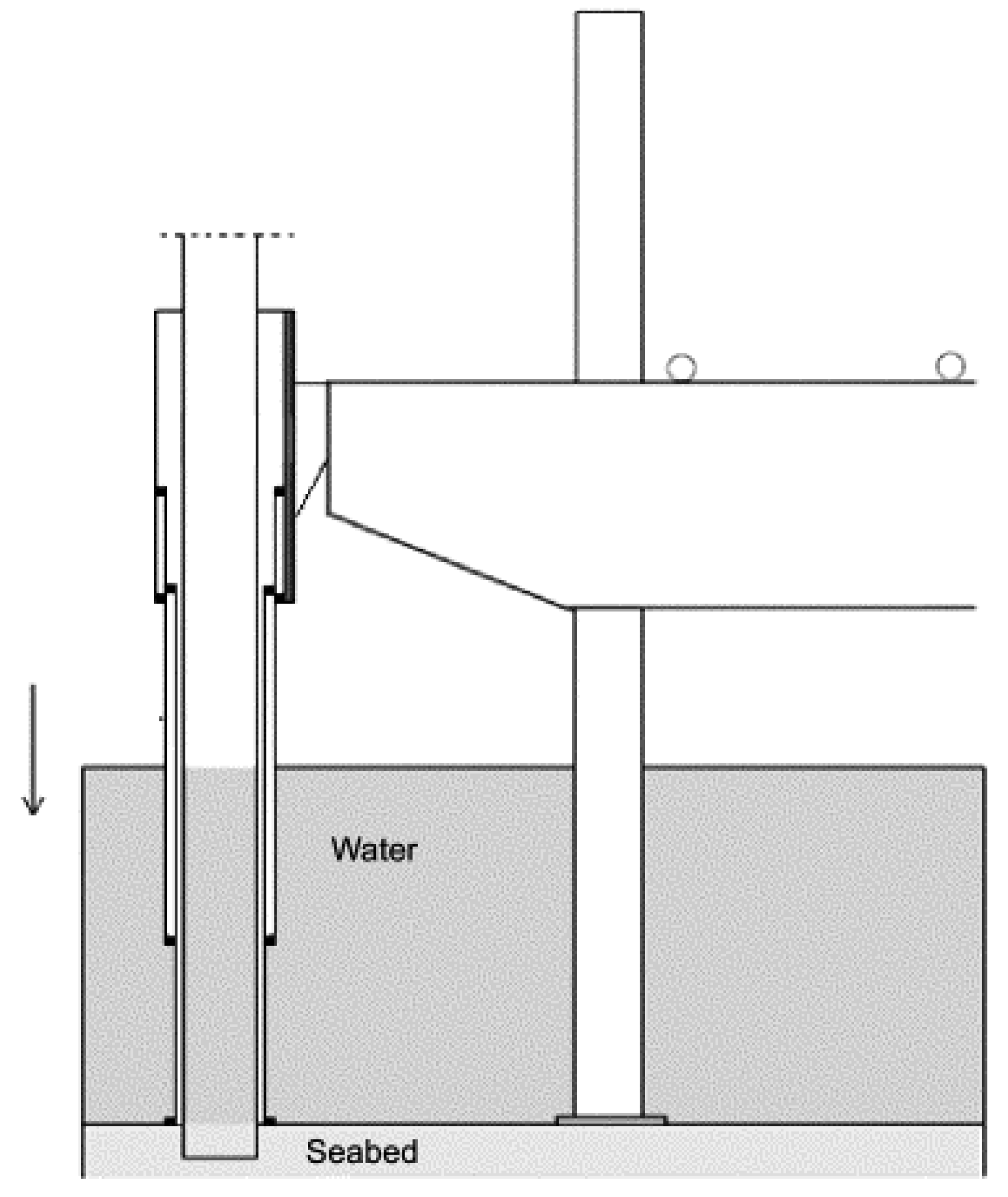
([4]). A cofferdam is an engineering design optimization problem. It is a prominent structure to attach a trivial submerged area to permit building a permanent structure on an allocated site. The cofferdam function is elicited in a random environment by transitions in surrounding water levels. The architecture designs a dam of height $x_1$, length $x_2$ breadth $x_3$, and total required perimeter $x_4$ and intends to estimate the most promising total cost for making decisions. The RHS parameters can be of any simplex dimensions such as area, volume, etc., which is not quite certain. These are no longer crisp or deterministic, but the allowable lower and upper bounds over each area/volume are determined in the closed interval. Thus, the use of varying parameters is quite worthwhile and the decision under such variation will be helpful in determining the range of optimal outcomes. Figure 1 depicts an illustrative example of a cofferdam.

Thus, the equivalent mathematical programming problem with varying parameters is given as follows (27):

$$\begin{array}{cc}\mathrm{F}=\underset{x}{\mathrm{Minimize}}\hfill & 2x_1^{-0.9}{x}_2^{-1.5}{x}_3^{-1}{x}_4^{-1.6}+4x_1^{-1}{x}_2^{-1}{x}_3^{-0.1}{x}_4^{-1}\hfill \\ \mathrm{s}.\mathrm{x}.\hfill & \\ \hfill & 2x_1^{-2}{x}_2^{-1}{x}_3^2{x}_4+1.6x_1{x}_3{x}_4^2\le {\tilde{B}}_1\hfill \\ \hfill & 1.9x_1^2{x}_2^{1.4}{x}_3{x}_4+3.1x_1^{2.2}{x}_4\le {\tilde{B}}_2\hfill \\ \hfill & x_1,x_2,x_3,x_4\ge 0.\hfill \end{array}$$

(27)

where ${\tilde{B}}_1\in (3,3.2)$ and ${\tilde{B}}_2\in (2,2.4)$ are the varying parameters. Since all the parameters are crisp except the RHS, then Problems (23) and (26) can be utilized to obtain the upper and lower bounds of the objective values in Problem (27). According to Problems (23) and (26), the formulations of the upper and lower bounds for Problem (27) can be presented as follows:

$$\begin{array}{cc}\mathbf{Model}\mathbf{A}\hfill & \\ \underline{F}=\underset{y}{\mathrm{Minimize}}\hfill & {\left({\displaystyle \frac{2}{y_{01}}}\right)}^{y_{01}}{\left({\displaystyle \frac{4}{y_{02}}}\right)}^{y_{02}}{\left({\displaystyle \frac{2y_{10}}{{\tilde{B}}_1{y}_{11}}}\right)}^{y_{11}}{\left({\displaystyle \frac{1.6y_{10}}{{\tilde{B}}_1{y}_{12}}}\right)}^{y_{12}}{\left({\displaystyle \frac{1.9y_{20}}{{\tilde{B}}_2{y}_{21}}}\right)}^{y_{21}}{\left({\displaystyle \frac{3.1y_{20}}{{\tilde{B}}_2{y}_{22}}}\right)}^{y_{22}}\hfill \\ \mathrm{s}.\mathrm{x}.\hfill & \\ \hfill & y_{01}+y_{02}=1,\hfill \\ \hfill & y_{01}+y_{02}-2y_{11}+y_{12}+2y_{21}+2.2y_{22}=0,\hfill \\ \hfill & y_{01}-y_{02}-y_{11}+1.4y_{21}=0,\hfill \\ \hfill & -y_{01}+y_{02}+2y_{11}+y_{12}+y_{21}=0,\hfill \\ \hfill & y_{01}-y_{02}+y_{11}+2y_{12}+y_{21}+y_{22}=0,\hfill \\ \hfill & y_{01},y_{02},y_{11},y_{21},y_{12},y_{22}\ge 0\hfill \\ \hfill & 3\le {\tilde{B}}_1\le 3.2,2\le {\tilde{B}}_2\le 2.4,\forall i=1,2,\cdots ,m.\hfill \end{array}$$

(28)

and

$$\begin{array}{cc}\mathbf{Model}\mathbf{B}\hfill & \\ \hfill & \\ \overline{F}=\underset{y}{\mathrm{Maximize}}\hfill & {\left({\displaystyle \frac{2}{y_{01}}}\right)}^{y_{01}}{\left({\displaystyle \frac{4}{y_{02}}}\right)}^{y_{02}}{\left({\displaystyle \frac{2y_{10}}{{\tilde{B}}_1{y}_{11}}}\right)}^{y_{11}}{\left({\displaystyle \frac{1.6y_{10}}{{\tilde{B}}_1{y}_{12}}}\right)}^{y_{12}}{\left({\displaystyle \frac{1.9y_{20}}{{\tilde{B}}_2{y}_{21}}}\right)}^{y_{21}}{\left({\displaystyle \frac{3.1y_{20}}{{\tilde{B}}_2{y}_{22}}}\right)}^{y_{22}}\hfill \\ \mathrm{s}.\mathrm{x}.\hfill & \\ \hfill & y_{01}+y_{02}=1,\hfill \\ \hfill & y_{01}+y_{02}-2y_{11}+y_{12}+2y_{21}+2.2y_{22}=0,\hfill \\ \hfill & y_{01}-y_{02}-y_{11}+1.4y_{21}=0,\hfill \\ \hfill & -y_{01}+y_{02}+2y_{11}+y_{12}+y_{21}=0,\hfill \\ \hfill & y_{01}-y_{02}+y_{11}+2y_{12}+y_{21}+y_{22}=0,\hfill \\ \hfill & y_{01},y_{02},y_{11},y_{21},y_{12},y_{22}\ge 0\hfill \\ \hfill & 3\le {\tilde{B}}_1\le 3.2,2\le {\tilde{B}}_2\le 2.4,\forall i=1,2,\cdots ,m.\hfill \end{array}$$

(29)

Thus, Problems (28) and (29) are the required upper and lower bounds for the geometric programming problem (27). Upon solving the problem at zero degree of difficulty, the upper and lower bounds for the objective functions are obtained as $\overline{F}=8.5429$ and $\underline{F}=4.9271$, respectively. However, the objective values at ${\tilde{B}}_1=3.2$ and ${\tilde{B}}_2=2.4$ are found to be $\tilde{F}=5.6212$. Therefore, the obtain objective function lies between the range of the upper and lower bounds, which shows that it is justified to reduce the objective values at the maximum RHS under variations.

Example 2

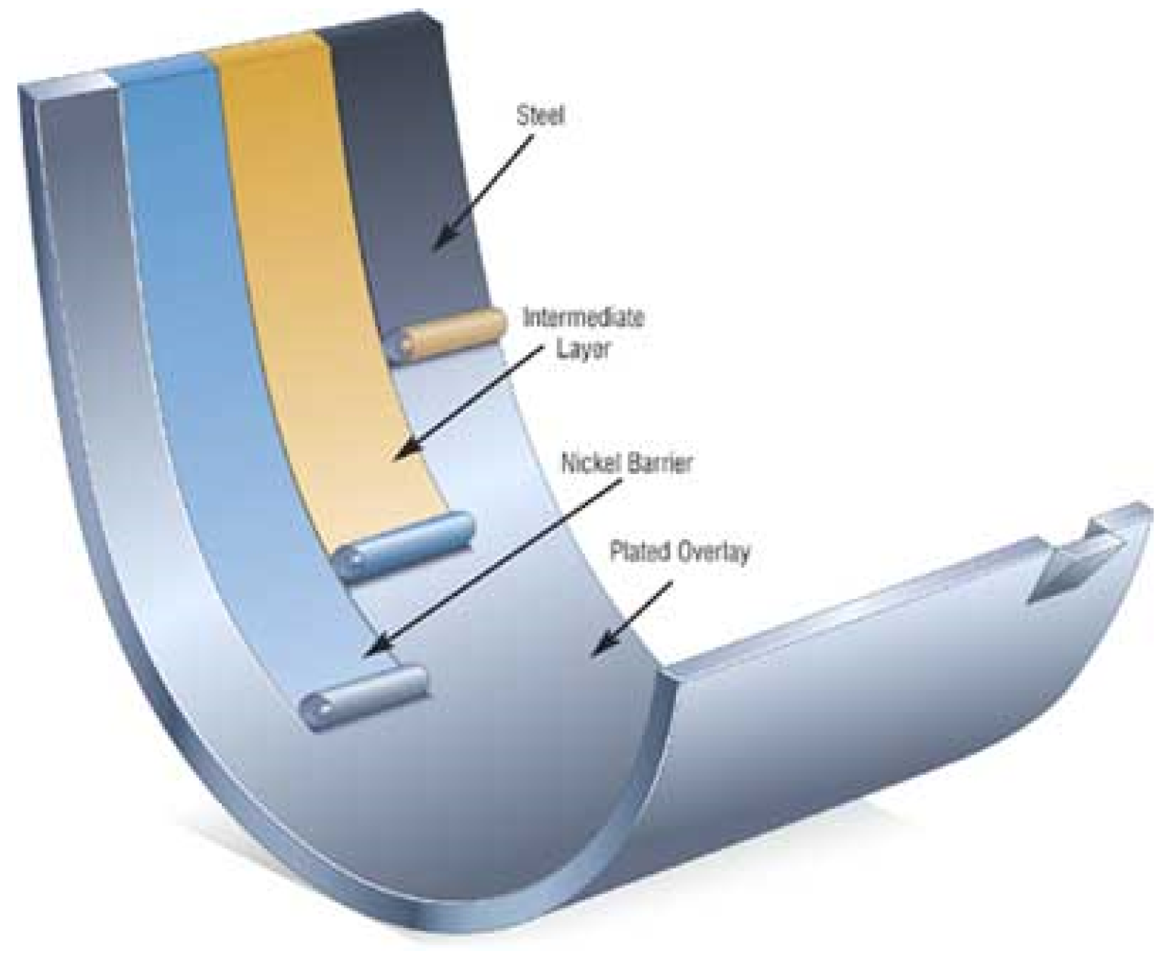
([4]). This illustration belongs to a design problem of a journal bearing. The texture of the journal bearing is an inverse problem, where the eccentricity ratio and attitude angle are obtained for a defined load and speed. The engineers may not have experience in modeling the structure of this new type of journal bearing. The volume of steel, the thickness of the intermediate layer and nickel barrier, and the dimension of the plated overlay of the journal bearing are assumed to be unknown. Thus, the values of these parameters have been depicted between some specified closed intervals and taken in the form of lower and upper bounds, respectively. Hence, the varying solution outcomes will also come by ensuring the optimal objectives between corresponding intervals. Figure 2 represents the structure of the journal bearing used in this example. Hence, some parameters of the model are approximately known and are estimated by the engineers. Suppose that $x_1$ is the radial clearance, $x_2$ the fluid force, $x_3$ the diameter, $x_4$ the rotation speed, and $x_5$ the length-to-diameter ratio.

The following mathematical programming formulation can depict the design problem as a geometric programming problem (30):

$$\begin{array}{cc}\mathrm{F}=\underset{x}{\mathrm{Minimize}}\hfill & 0.5x_1^2{x}_2{x}_4{x}_5+1.1x_1^{-1}{x}_2^{-1}{x}_3^{-1}\hfill \\ \mathrm{s}.\mathrm{x}.\hfill & \\ \hfill & 8.4x_1{x}_2^{-1}{x}_3^{-1}{x}_4^{-1}{x}_5\le {\tilde{B}}_1\hfill \\ \hfill & 0.5x_2{x}_3+x_1{x}_4^{-1}{x}_5^{-1}+1.6x_3{x}_4\le {\tilde{B}}_2\hfill \\ \hfill & x_1,x_2,x_3,x_4,x_5\ge 0.\hfill \end{array}$$

(30)

where ${\tilde{B}}_1\in (4,4.2)$ and ${\tilde{B}}_2\in (0,1)$ are the varying parameters. Since all the parameters are crisp except the RHS, then Problems (23) and (26) can be utilized to obtain the upper and lower bound of the objective values in Problem (30). According to the problems (23) and (26), the formulations of the upper and lower bounds for Problem (30) can be presented as follows (31):

$$\begin{array}{cc}\mathbf{Model}\mathbf{A}\hfill & \\ \underline{F}=\underset{y}{\mathrm{Minimize}}\hfill & {\left({\displaystyle \frac{0.5}{y_{01}}}\right)}^{y_{01}}{\left({\displaystyle \frac{1.1}{y_{02}}}\right)}^{y_{02}}{\left({\displaystyle \frac{8.4}{{\tilde{B}}_1}}\right)}^{y_{11}}{\left({\displaystyle \frac{8.4}{{\tilde{B}}_2}}\right)}^{y_{11}}{\left({\displaystyle \frac{0.5y_{20}}{y_{21}}}\right)}^{y_{21}}{\left({\displaystyle \frac{y_{20}}{y_{22}}}\right)}^{y_{22}}{\left({\displaystyle \frac{1.6y_{20}}{y_{23}}}\right)}^{y_{23}}\hfill \\ \mathrm{s}.\mathrm{x}.\hfill & \\ \hfill & y_{01}+y_{02}=1,\hfill \\ \hfill & 2y_{01}-y_{02}+y_{11}+y_{22}=0,\hfill \\ \hfill & y_{01}-y_{02}-y_{11}+y_{21}=0,\hfill \\ \hfill & -y_{02}-y_{11}+y_{21}+y_{23}=0,\hfill \\ \hfill & y_{01}-y_{11}-y_{22}+y_{23}=0,\hfill \\ \hfill & y_{01}+y_{11}-y_{22}=0,\hfill \\ \hfill & y_{01},y_{02},y_{11},y_{21},y_{22},y_{23}\ge 0\hfill \\ \hfill & 4\le {\tilde{B}}_1\le 4.2,0\le {\tilde{B}}_2\le 1,\forall i=1,2,\cdots ,m.\hfill \end{array}$$

(31)

where $y_{21}+y_{22}+y_{23}=y_{20}$ and the upper bound can be stated as follows (32):

$$\begin{array}{cc}\mathbf{Model}\mathbf{B}\hfill & \\ \overline{F}=\underset{y}{\mathrm{Maximize}}\hfill & {\left({\displaystyle \frac{0.5}{y_{01}}}\right)}^{y_{01}}{\left({\displaystyle \frac{1.1}{y_{02}}}\right)}^{y_{02}}{\left({\displaystyle \frac{8.4}{{\tilde{B}}_1}}\right)}^{y_{11}}{\left({\displaystyle \frac{8.4}{{\tilde{B}}_2}}\right)}^{y_{11}}{\left({\displaystyle \frac{0.5y_{20}}{y_{21}}}\right)}^{y_{21}}{\left({\displaystyle \frac{y_{20}}{y_{22}}}\right)}^{y_{22}}{\left({\displaystyle \frac{1.6y_{20}}{y_{23}}}\right)}^{y_{23}}\hfill \\ \mathrm{s}.\mathrm{x}.\hfill & \\ \hfill & y_{01}+y_{02}=1,\hfill \\ \hfill & 2y_{01}-y_{02}+y_{11}+y_{22}=0,\hfill \\ \hfill & y_{01}-y_{02}-y_{11}+y_{21}=0,\hfill \\ \hfill & -y_{02}-y_{11}+y_{21}+y_{23}=0,\hfill \\ \hfill & y_{01}-y_{11}-y_{22}+y_{23}=0,\hfill \\ \hfill & y_{01}+y_{11}-y_{22}=0,\hfill \\ \hfill & y_{01},y_{02},y_{11},y_{21},y_{22},y_{23}\ge 0\hfill \\ \hfill & 4\le {\tilde{B}}_1\le 4.2,0\le {\tilde{B}}_2\le 1,\forall i=1,2,\cdots ,m.\hfill \end{array}$$

(32)

where $y_{21}+y_{22}+y_{23}=y_{20}$.

The above Problems (31) and (32) provide the required upper and lower bound for the problem (30). Both of these problems are concave programming problems with linear constraints. Upon solving the problem at zero degree of difficulty, the upper and lower bounds for the objective functions are obtained as $\overline{F}=4.314$ and $\underline{F}=3.045$, respectively. However, the objective values at ${\tilde{B}}_1=4.2$ and ${\tilde{B}}_2=1$ are found to be $\tilde{F}=3.561$. Therefore, the obtain objective function lies between the range of the upper and lower bounds, which shows that it is justified to reduce the objective values at the maximum RHS under variations.

4.1. Application to System Reliability Optimization

Assume system reliability having n components connected in series. Suppose $r_i(i=1,2,\cdots ,n)$ represents the individual reliability of the i-th component of the system. Similarly, $R_s(r_1,r_2,\cdots ,r_n)$ is the reliability of the whole series system. Consequently, $C_s(r_1,r_2,\cdots ,r_n)$ depicts the total cost of n components associated with the system reliability. It seldom happens that the system reliability is maximized when the cost of the associated system is exactly known; however, some varying cost may make it easier to execute the smooth function of the framework. The obtained lower and upper bounds on the cost objective function will ensure the variation in total cost associated with the system and help with allocating the budget for maintenance or renovation, etc. In the same manner, minimizing the system cost under the varying reliability of the whole system would be quite a worthwhile task. The minimization of the system cost without affecting the system reliability is much needed to ensure the longer performance of the components. Thus, we considered that the system reliability is varying between some specified intervals and bounded by upper and lower bounds. This situation is quite common due to uncertainty in the failure of any components. In real-life scenarios, the minimization of the total system cost by maintaining the system reliability would be a more prominent modeling texture of the reliability optimization problems (see [17,29,30]). Therefore, the mathematical model for the minimization of system cost under varying system reliability takes the form of the geometric programming problem and can be represented as follows (33):

$$\begin{array}{cc}\mathrm{F}=\mathrm{Minimize}\hfill & C_s(r_1,r_2,\cdots ,r_n)=+\sum _{i=1}^n{C}_i{r}_i^{{\alpha }_i}\hfill \\ \mathrm{s}.\mathrm{x}.\hfill & \\ \hfill & (r_1\times r_2\times \cdots \times r_n)=\prod _{i=1}^n{r}_i\ge {\tilde{R}}_s\hfill \\ \hfill & {\underline{R}}_s\le {\tilde{R}}_s\le {\overline{R}}_s\hfill \\ \hfill & 0\le r_i\le 1\forall i=1,2,\cdots ,n.\hfill \end{array}$$

(33)

where ${\alpha }_i$ is the acceptable tolerance linked with the i-th component. We considered the three components connected in series, and the relevant data are summarized in

Table 2. Input data for the system reliability optimization problem.

${\mathit{C}}_1$	${\mathit{C}}_2$	${\mathit{C}}_3$	${\mathit{\alpha }}_1$	${\mathit{\alpha }}_2$	${\mathit{\alpha }}_3$	${\underline{\mathit{R}}}_{\mathit{s}}\le {\tilde{\mathit{R}}}_{\mathit{s}}\le {\overline{\mathit{R}}}_{\mathit{s}}$
150	210	270	20	15	10	$0.6358\le {\tilde{R}}_s\le 0.9776$

.

Since all the parameters are crisp except the system reliability, then Problems (23) and (26) can be utilized to obtain the upper and lower bounds of the objective values in Problem (33). According to the problems (23) and (26), the formulations of the upper and lower bounds for Problem (33) can be presented as follows (34):

$$\begin{array}{cc}\mathbf{Model}\mathbf{A}\hfill & \\ \underline{F}=\underset{y}{\mathrm{Minimize}}\hfill & {\left({\displaystyle \frac{150}{y_{01}}}\right)}^{y_{01}}{\left({\displaystyle \frac{210}{y_{02}}}\right)}^{y_{02}}{\left({\displaystyle \frac{270}{y_{03}}}\right)}^{y_{03}}{\left({\displaystyle \frac{1}{{\tilde{R}}_s{y}_{11}}}\right)}^{y_{11}}{\left({\displaystyle \frac{1}{{\tilde{R}}_s{y}_{12}}}\right)}^{y_{12}}{\left({\displaystyle \frac{1}{{\tilde{R}}_s{y}_{13}}}\right)}^{y_{13}}\hfill \\ \mathrm{s}.\mathrm{x}.\hfill & \\ \hfill & y_{01}+y_{02}+y_{03}=1,\hfill \\ \hfill & 20y_{01}+15y_{02}+10y_{03}+y_{11}+y_{12}+y_{13}=0,\hfill \\ \hfill & y_{01}-y_{02}-y_{03}+y_{11}+y_{12}+y_{13}=0,\hfill \\ \hfill & y_{01},y_{02},y_{03},y_{11},y_{12},y_{13}\ge 0\hfill \\ \hfill & 0.6358\le {\tilde{R}}_s\le 0.9776,\forall i=1,2,3.\hfill \end{array}$$

(34)

whereas the upper bound can be stated as follows (35):

$$\begin{array}{cc}\mathbf{Model}\mathbf{B}\hfill & \\ \overline{F}=\underset{y}{\mathrm{Maximize}}\hfill & {\left({\displaystyle \frac{150}{y_{01}}}\right)}^{y_{01}}{\left({\displaystyle \frac{210}{y_{02}}}\right)}^{y_{02}}{\left({\displaystyle \frac{270}{y_{03}}}\right)}^{y_{03}}{\left({\displaystyle \frac{1}{{\tilde{R}}_s{y}_{11}}}\right)}^{y_{11}}{\left({\displaystyle \frac{1}{{\tilde{R}}_s{y}_{12}}}\right)}^{y_{12}}{\left({\displaystyle \frac{1}{{\tilde{R}}_s{y}_{13}}}\right)}^{y_{13}}\hfill \\ \mathrm{s}.\mathrm{x}.\hfill & \\ \hfill & y_{01}+y_{02}+y_{03}=1,\hfill \\ \hfill & 20y_{01}+15y_{02}+10y_{03}+y_{11}+y_{12}+y_{13}=0,\hfill \\ \hfill & y_{01}-y_{02}-y_{03}+y_{11}+y_{12}+y_{13}=0,\hfill \\ \hfill & y_{01},y_{02},y_{03},y_{11},y_{12},y_{13}\ge 0\hfill \\ \hfill & 0.6358\le {\tilde{R}}_s\le 0.9776,\forall i=1,2,3.\hfill \end{array}$$

(35)

The above problems (34) and (35) provide the required upper and lower bound for the problem (33). Upon solving the problem at zero degree of difficulty, the upper and lower bounds for the system cost are obtained as $\overline{C_s}=521.95$ and $\underline{C_s}=216.35$, respectively. However, the system cost at ${\tilde{R}}_s=0.88$ is found to be $\widetilde{C_s}=351.29$. Therefore, the obtained system cost lies between the range of its upper and lower bounds, which shows that it is justified to reduce the system cost at maximum system reliability under variations.

4.2. Analyses of Computational Complexity and Discussions

This proposed bounded solution method captures the behavior of varying parameters and provides the interval-based solution of the objective function. Most often, uncertain parameters exist in any form, such as they may take the form of randomness, fuzziness, and any other aspects of uncertainty. The uncertainty among parameters arises due to vagueness being able to be dealt with by using fuzzy approaches, whereas the stochastic technique is applied when the uncertainty involves randomness among the parameters. More precisely, contrary to other uncertain optimization approaches, the developed approach adheres to comparatively less computational complexity in the sense of mathematical computation (e.g., some mathematical calculations are used to derive the crisp or deterministic version of fuzzy or random parameters), and there is no scope for obtaining the deterministic version of the problem for such varying geometric programming problems. The beauty of the proposed method can be highlighted by the fact that sensitivity analyses (post-optimality analysis) doe not need to be performed because the continuous variations among the parametric values directly produce the range of optimal objective functions from the interval parameters. Thus, the propounded solution approach can be the most prominent and efficient decision-maker while dealing with uncertain parameters other than the fuzzy or stochastic form.

The generalization of the conventional geometric programming problem of constant parameters is highlighted for interval parameters. The most prominent and extensive idea is to determine the lower and upper bounds of the range by applying the two-level mathematical programming technique to geometric programming problems. With the aid of a strong duality theorem, the two-level geometric programming problems are converted into a pair of one-level geometric programming problems to implement the computational study. When all the varying parameters degenerate to constant parameters, the two-level geometric programming problem turns into the conventional geometric programming problem. In general, in interval geometric programming problems, it may probably happen that the problem is infeasible for some specified range of varying parameters. Thus, our proposed methods are free from infeasibility and ignore those complexities due to infeasible values. The proposed method obtains the lower and upper bounds of the feasible solutions directly. In addition, the suggested method does not examine the range of values that results in infeasibility. Furthermore, developing two-level geometric programming problems can determine the lower and upper bounds of the objective values. However, mathematical programming is nonlinear in the case of geometric programming problems, which may be very typical for solving large-scale problems. The comparative study is presented in

Table 3. Comparison between the proposed method and traditional methods.

Proposed Method	Traditional Methods
(1) Deals with the varying parameters	No scope for dealing with such parameters
(2) No need to consider the fuzzy or random parameters while dealing with uncertainty	It may require the fuzzy or random parameters while dealing with uncertainty
(3) No need to obtain the crisp or deterministic version of uncertain models	It requires the crisp or deterministic version of the uncertain models
(4) Sensitivity or post-optimal analysis is not required for the obtained solutions	Sensitivity or post-optimal analysis can be performed separately
(5) Less computational complexity in terms of mathematical calculations	Comparatively involves more computational complexity in terms of mathematical calculations

.

The presented work can be described as an empirical case research work by filling the various gaps [8,9,17,19,29] such as instant variation among parameters, two-level mathematical programming, duality theory in the GPP, and the automatic post-optimal analysis metric. In system reliability modeling, various parameters can be taken as varying between some specified intervals. For example, the cofferdam, shaft, journal bearings, etc., are the raw parts that are the building block materials of the various products and machines. This means that the parameters can be taken as uncertain, and using some specified tools, they can be converted into a crisp one. In the literature, the concept of fuzzy and random parameters is available, which deals with the vagueness and randomness in the parameters. However, we have provided an opportunity to define the parameters under the continuous variations bounded by upper and lower limits. Instead of taking the vague and random parameters, one can assume the continuous variations in the parameters’ values can be tackled with the two-level mathematical programming techniques discussed in this paper. Additionally, the sensitivity and post-optimality of the obtained solution results are waived off due to the working procedure of the proposed approach.

In the future, a solution method that involves all the parameters under variation in the geometric programming formulation is much required to ensure solvability. The values near the lower and upper bounds have a significantly lower probability of occurrence. If the distributions of varying data are known in the stochastic environment, then the distribution of the objective function would be obtained, which is more realistic, and the scenario is generated for consequent decision-making. Therefore, this lays down another direction for future research by deriving the distribution of the objective functions based on the distributions of the varying parameters.

5. Conclusions

The geometric programming problem is an integrated part of mathematical programming and has real-life applications in many engineering problems such as gravel-box design, bar–truss region texture, system reliability optimization, etc. The concept of varying parameters under the objective functions is discussed with the aim that uncertainty is critically involved and affects engineering problems’ formulations directly. The propounded research work is developed and introduces an interval-based solution approach to finding the upper and lower limits on the objective function of the varying parameters. The outer- and inner-level geometric programming problem is transformed into a single-level mathematical programming problem. The outcomes are summarized in the numerical illustrations and observed in the precise interval where they should exist. The system reliability optimization problem also provides evidence of the discussed problem’s successful implementation and dynamic solution results. The minimum system cost is obtained at the utmost system reliability, which also falls into the lower and upper bounds of the system costs.

The scope of usual sensitivity analysis is not further required due to the flexible nature of the proposed solution method. The propounded approach allows the abrupt fluctuations among the parameters between given intervals for which bounds over the objective functions are directly obtained. It also makes the computational algorithm easier than other methods by ignoring the uncertain parameters such as fuzzy, stochastic, and other uncertain forms that yield a solution procedure that is comparatively more complex. The developed approach may be extended for future research to stochastic programming, bi-level or multilevel programming, and various engineering problems with real-life applications.

References

- Duffin, R.; Peterson, E.L. Duality theory for geometric programming. SIAM J. Appl. Math. 1966, 14, 1307–1349. [Google Scholar] [CrossRef]
- Duffin, R.J. Linearizing geometric programs. SIAM Rev. 1970, 12, 211–227. [Google Scholar] [CrossRef] [Green Version]
- Duffin, R.J.; Peterson, E.L. Reversed geometric programs treated by harmonic means. Indiana Univ. Math. J. 1972, 22, 531–550. [Google Scholar] [CrossRef]
- Rao, S.S. Engineering Optimization: Theory and Practice; John Wiley & Sons: Hoboken, NJ, USA, 2019. [Google Scholar]
- Liu, S.T. Fuzzy measures for profit maximization with fuzzy parameters. J. Comput. Appl. Math. 2011, 236, 1333–1342. [Google Scholar] [CrossRef] [Green Version]
- Lu, T.; Liu, S.T. Fuzzy nonlinear programming approach to the evaluation of manufacturing processes. Eng. Appl. Artif. Intell. 2018, 72, 183–189. [Google Scholar] [CrossRef]
- Ahmad, F.; Adhami, A.Y. Total cost measures with probabilistic cost function under varying supply and demand in transportation problem. Opsearch 2019, 56, 583–602. [Google Scholar] [CrossRef]
- Chakraborty, D.; Chatterjee, A.; Aishwaryaprajna. Multi-objective Fuzzy Geometric Programming Problem Using Fuzzy Geometry. In Trends in Mathematics and Computational Intelligence; Springer: Berlin/Heidelberg, Germany, 2019; pp. 123–129. [Google Scholar]
- Garg, H.; Rani, M.; Sharma, S.; Vishwakarma, Y. Intuitionistic fuzzy optimization technique for solving multi-objective reliability optimization problems in interval environment. Expert Syst. Appl. 2014, 41, 3157–3167. [Google Scholar] [CrossRef]
- Islam, S.; Roy, T.K. Modified geometric programming problem and its applications. J. Appl. Math. Comput. 2005, 17, 121–144. [Google Scholar] [CrossRef]
- Islam, S.; Roy, T.K. A new fuzzy multi-objective programming: Entropy based geometric programming and its application of transportation problems. Eur. J. Oper. Res. 2006, 173, 387–404. [Google Scholar] [CrossRef]
- Islam, S.; Mandal, W.A. Preliminary Concepts of Geometric Programming (GP) Model. In Fuzzy Geometric Programming Techniques and Applications; Springer: Berlin/Heidelberg, Germany, 2019; pp. 1–25. [Google Scholar]
- Islam, S.; Mandal, W.A. Geometric Programming Problem Under Uncertainty. In Fuzzy Geometric Programming Techniques and Applications; Springer: Berlin/Heidelberg, Germany, 2019; pp. 287–330. [Google Scholar]
- Islam, S.; Mandal, W.A. Fuzzy Unconstrained Geometric Programming Problem. In Fuzzy Geometric Programming Techniques and Applications; Springer: Berlin/Heidelberg, Germany, 2019; pp. 133–153. [Google Scholar]
- Islam, S.; Mandal, W.A. Intuitionistic and Neutrosophic Geometric Programming Problem. In Fuzzy Geometric Programming Techniques and Applications; Springer: Berlin/Heidelberg, Germany, 2019; pp. 331–355. [Google Scholar]
- Khorsandi, A.; Cao, B.Y.; Nasseri, H. A New Method to Optimize the Satisfaction Level of the Decision Maker in Fuzzy Geometric Programming Problems. Mathematics 2019, 7, 464. [Google Scholar] [CrossRef] [Green Version]
- Mahapatra, G.; Roy, T.K. Fuzzy multi-objective mathematical programming on reliability optimization model. Appl. Math. Comput. 2006, 174, 643–659. [Google Scholar] [CrossRef]
- Negi, G.; Kumar, A.; Pant, S.; Ram, M. Optimization of complex system reliability using hybrid grey wolf optimizer. Decis. Mak. Appl. Manag. Eng. 2021, 4, 241–256. [Google Scholar] [CrossRef]
- Roustaee, M.; Kazemi, A. Multi-objective stochastic operation of multi-microgrids constrained to system reliability and clean energy based on energy management system. Electr. Power Syst. Res. 2021, 194, 106970. [Google Scholar] [CrossRef]
- Zolfaghari, S.; Mousavi, S.M. A novel mathematical programming model for multi-mode project portfolio selection and scheduling with flexible resources and due dates under interval-valued fuzzy random uncertainty. Expert Syst. Appl. 2021, 182, 115207. [Google Scholar] [CrossRef]
- Sedaghat, N.; Ardakan, M.A. G-mixed: A new strategy for redundant components in reliability optimization problems. Reliab. Eng. Syst. Saf. 2021, 216, 107924. [Google Scholar] [CrossRef]
- Meng, Z.; Ren, S.; Wang, X.; Zhou, H. System reliability-based design optimization with interval parameters by sequential moving asymptote method. Struct. Multidiscip. Optim. 2021, 63, 1767–1788. [Google Scholar] [CrossRef]
- Kugele, A.S.H.; Ahmed, W.; Sarkar, B. Geometric programming solution of second degree difficulty for carbon ejection controlled reliable smart production system. RAIRO Oper. Res. 2022, 56, 1013–1029. [Google Scholar] [CrossRef]
- Son, Y.; Mukherjee, S.; Mallik, R.; Majmunovi’c, B.; Dutta, S.; Johnson, B.; Maksimović, D.; Seo, G.S. Levelized Cost of Energy-Oriented Modular String Inverter Design Optimization for PV Generation System Using Geometric Programming. IEEE Access 2022, 10, 27561–27578. [Google Scholar] [CrossRef]
- Shen, K.; Yu, W.; Chen, X.; Khosravirad, S.R. Energy Efficient HARQ for Ultrareliability via a Novel Outage Probability Bound and Geometric Programming. IEEE Trans. Wirel. Commun. 2022. [Google Scholar] [CrossRef]
- Rajamony, R.; Wang, S.; Navaratne, R.; Ming, W. Multi-objective design of single-phase differential buck inverters with active power decoupling. IEEE Open J. Power Electron. 2022, 3, 105–114. [Google Scholar] [CrossRef]
- Singh, G.; Singh, A.K. Optimizing multi-VM migration by allocating transfer and compression rate using geometric programming. Simul. Model. Pract. Theory 2021, 106, 102201. [Google Scholar] [CrossRef]
- Server, N. State-of-the-Art Solvers for Numerical Optimization. 2016. Available online: https://neos-server.org/neos/ (accessed on 22 June 2022).
- Kundu, T.; Islam, S. Neutrosophic goal geometric programming problem and its application to multi-objective reliability optimization model. Int. J. Fuzzy Syst. 2018, 20, 1986–1994. [Google Scholar] [CrossRef]
- Ahmad, F.; Adhami, A.Y. Spherical Fuzzy Linear Programming Problem. In Decision Making with Spherical Fuzzy Sets; Springer: Berlin/Heidelberg, Germany, 2021; pp. 455–472. [Google Scholar]
Figure 1.
Illustrative figure of a cofferdam.
Figure 2.
Illustrative figure of a journal bearing.