Testing for the Presence of the Leverage Effect without Estimation

Abstract

Problem: The leverage effect plays an important role in finance. However, the statistical test for the presence of the leverage effect is still lacking study. Approach: In this paper, by using high frequency data, we propose a novel procedure to test if the driving Brownian motion of an It$\widehat{\mathrm{o}}$ semi-martingale is correlated to its volatility (referred to as the leverage effect in financial econometrics) over a long time period. The asymptotic setting is based on observations within a long time interval with the mesh of the observation grid shrinking to zero. We construct a test statistic via forming a sequence of Studentized statistics whose distributions are asymptotically normal over blocks of a fixed time span, and then collect the sequence based on the whole data set of a long time span. Result: The asymptotic behaviour of the Studentized statistics was obtained from the cubic variation of the underlying semi-martingale and the asymptotic distribution of the proposed test statistic under the null hypothesis that the leverage effect is absent was established, and we also show that the test has an asymptotic power of one against the alternative hypothesis that the leverage effect is present. Implications: We conducted extensive simulation studies to assess the finite sample performance of the test statistics, and the results show a satisfactory performance for the test. Finally, we implemented the proposed test procedure to a dataset of the SP500 index. We see that the null hypothesis of the absence of the leverage effect is rejected for most of the time period. Therefore, this provides a strong evidence that the leverage effect is a necessary ingredient in modelling high-frequency data.

1. Introduction

The leverage effect in financial economics refers to the correlation between the driven system of an asset price and its volatility. It is widely accepted that the leverage effect is a common stylized fact of financial data, like the skewed distribution, volatility asymmetry, etc. Moreover, empirical analyses have provided evidence that the returns of equities are usually negatively correlated to the near future volatility. Ang and Chen [1] found that volatility rises when stock prices go down and that volatility decreases if stock prices go up, see also Black [2], Christie [3].

The existence of the leverage effect is explained from an economic point of view, firstly. For example, Modigliani and Miller [4] linked the leverage effect to the financial leverage of a firm, namely, the debt–equity ratio, which reflects a firm’s capital structure. Using the idea of leverage well demonstrates the negative leverage effect usually found in financial data. Precisely, with an increase in the stock price, the value of equity increases more than the value of debt because the claims of the debt holders are limited in a short time interval; thus, its leverage (debt to equity ratio) decreases; hence, the firm will be less risky, which results in a drop in the volatility. The same logic applies to falling stock prices, which should lead to an increase in future volatility. However, the financial leverage is not the only driver for the price-volatility relation, there is also evidence that the leverage effect observed in financial time series is not fully explained by a firm’s leverage. Modigliani and Miller [4] found a strong leverage effect for falling stock prices but a very weak, even nonexistent, leverage effect for positive returns; Hens and Steude [5] and Hasanhodzic and Lo [6] found the leverage effect in many financial markets although the underlying asset did not exhibit any financial leverage at all.

The leverage effect characterizes the correlation between the latent process and the volatility process, since the volatility process is unobservable; hence, it has to be estimate with the observed data. For low-frequency data, it is hard to estimate unless assuming some stationary condition. However, for high-frequency data, it can be estimated more accurately. Therefore, the leverage effect can be more accurately measured in high-frequency data than low-frequency data. Recently, with help of widely available high-frequency financial data, the leverage effect can be quantitatively modelled and the statistical estimation of the leverage effect has been investigated. For example, Aït-Sahalia et al. [7] found that an estimator of the leverage effect using high-frequency data yields a “zero” estimator whatever the true value of the leverage effect is, based on the Heston’s stochastic volatility model and they created a bias-corrected consistent estimator; Wang and Mykland [8] considered the estimation of the leverage effect under the presence of microstructure noise; Aït-Sahalia et al. [9] further theoretically split the leverage effect into two parts: the continuous leverage effect and discontinuous leverage effect, which are the quadratic co-variations of continuous diffusion parts and jump parts of a volatility process and underlying-price process, respectively. Both leverage effects have been consistently estimated. They also showed the empirical evidence of the existence of the two kinds of leverage effects; Kalnina and Xiu [10] proposed a nonparametric model-free estimator for the leverage effect. The study provided two estimators for the leverage effect, the first one only uses the discretely observed stock-price data, as usual, while the second estimator also employs VIX data as the observation of the volatility process to improve estimation efficiency.

Despite the economic rationale and non-zero measure of the leverage effect in empirical analysis for most financial markets and equities, there is yet no theoretically valid test to tell whether it indeed exists under a given nominal level. If one wants to test the non-zero leverage effect, a natural way is to estimate the leverage effect first and then use the asymptotic normality (Studentized version) of the estimator to construct the confidence intervals. As the volatility is totally unobservable, we must estimate the volatility in advance, and then, based on these “estimated data” of the volatility and observed price data, we can compute the estimator of leverage effect, as stated in the above literature. This procedure, although theoretically feasible, must have a very slow convergence rate, which pays for the two estimation procedures ahead of the test statistic.

Mathematically speaking, we consider a continuous-time semi-martingale:

$$d{X}_t=b_{t}dt+{\sigma }_{t}d{W}_t,$$

(1)

where W is a standard Brownian motion defined on an appropriate probability space, and b and $\sigma$ are two processes satisfying some regular conditions (specified later), so that the stochastic differential equation is well-defined. The quantity of interest is the correlation between the two processes $\sigma$ and X, precisely, the quadratic co-variation ${\langle X,{\sigma }^2\rangle }_t.$ In this paper, we provide a simple and easy-ito-mplement testing procedure in which we do not need to estimate the leverage effect. Precisely, we assume that the volatility process further follows a continuous semi-martingale:

$$d{\sigma }_t=a_{t}dt+L_{t}d{W}_t+H_{t}d{B}_t,$$

(2)

where W is the driven Brownian motion of X and B is another standard Brownian motion, independent of W. Under this framework, we can see that $L_t\equiv 0$ indicates the absence of the leverage effect. Therefore, it is necessary to find statistics whose limit is an explicit function of L. For instance, we can firstly estimate it by the method in either Wang and Mykland [8] or Aït-Sahalia et al. [9], and then create the test statistics from a related central limit theorem. Here, instead of estimating first and testing afterwards, we create a direct test procedure. Kinnebrock and Podolskij [11] derived the following limiting result for the cubic variation of semi-martingale:

$$\begin{array}{ccc}\hfill \frac{1}{{\Delta }_n}\sum _{i=1}^n{\left({\Delta }_i^{n}X\right)}^3& {\to }^{\mathcal{S}}& 3{\int }_0^T{L}_s{\sigma }_s^{2}ds+3{\int }_0^T{\sigma }_s^{2}d{X}_s+\sqrt{6}{\int }_0^T{\left|{\sigma }_s\right|}^{3}d{\tilde{W}}_s.\hfill \end{array}$$

From this limiting result, if $L\equiv 0$ (under the null hypothesis), the limit on the right-hand side is a conditional normal random variable. Moreover, the “conditional mean” $3{\int }_0^T{\sigma }_s^{2}d{X}_s$ can be consistently estimated, and the conditional variance can be consistently estimated as well. That is, after Studentization, it would result in a standard normal distribution asymptotically. Our analysis shows that this de-biased and Studentized statistic, although it indeed yields a satisfactory performance under the null hypothesis as expected, it does not provide a unit power under the alternative hypothesis. To improve the power, we consider the high-frequency data of a long time period—$[0,T]$, for instance—and then implement and replicate the procedure in each time interval $[k-1,k]$ for $k=1,\cdots ,T$, to obtain a sequence of asymptotically independent standard normal random variables. The final test statistic is constructed globally based on these independent standard normal random variables. We can show that this overall test procedure provides a unit power under the alternative hypothesis; the T is large. We establish the related asymptotic theory under both null and alternative hypotheses. The simulation studies assess the finite sample performance of the proposed test and show that the test provides satisfactory finite sample size and power. Finally, we also implement the procedure to test the presence of the leverage effect in modelling the SP500 index. The high-frequency dataset consists of the daily SP500 index in years 2000–2019, a total of 240 months. We consider the null hypothesis of the absence of the monthly leverage effect. The results show that the null hypothesis of zero monthly leverage effect is rejected for most of months. This supports the claim that the leverage effect is a necessary component in modelling high-frequency data.

The remainder of this paper is organized as follows. Section 2 contains the model setup and assumptions. In Section 3, we introduce some statistics and derive the related central limit theorem, based on which the test procedure is presented. Section 4 is the simulation studies and Section 5 is the application to a real high-frequency dataset. All the technical proofs are put into the Appendix A.

2. Setting and Assumptions

Let $\{X_t,t\ge 0\}$ denote the efficient log-price process defined on a filtered probability space $(\Omega ,\mathcal{F},{\mathcal{F}}_t,P)$ equipped with a filtration ${\left\{{\mathcal{F}}_t\right\}}_{t\ge 0}$ of the form:

$$d{X}_t=b_{t}dt+{\sigma }_{t}d{W}_t,$$

(3)

where, $b_t$ is a locally bounded and ${\mathcal{F}}_t$ progressively measurable real-valued process, ${\sigma }_t$ is a c$\stackrel{`}{a}$dl$\stackrel{`}{a}$g ${\mathcal{F}}_t$-adapted real-valued process, and $W_t$ is a ${\mathcal{F}}_t$-adapted Wiener process. This is the most popular model for log-price processes due to the consideration of no arbitrage, see Delbaen and Schachermayer [12,13,14]. Some future literature about the stochastic volatility models can be found in Stojkoski et al. [15], Zheng and Wang [16], Bouchaud and Potters [17], and Fouque et al. [18], and references therein.

We assume that the volatility process $\{{\sigma }_t,t\ge 0\}$ is of form:

$$d{\sigma }_t=a_{t}dt+L_{t}d{W}_t+H_{t}d{B}_t,$$

(4)

where, a, L and H are locally bounded and progressively measurable with respect to ${\mathcal{F}}_t$, and B is another ${\mathcal{F}}_t$-adapted Wiener process, independent of W.

Assumption 1.

The system satisfies (3) and (4), where X and σ are continuous processes. All the coefficients $b_t$, $a_t$, $L_t$ and $H_t$ are locally bounded in absolute value.

The problem of interest is to test:

$${\mathrm{H}}_0:L_t\equiv 0,\mu -a.s.vs.{\mathrm{H}}_1:L_t\not\equiv 0,\mu -a.s.,$$

(5)

where $\mu$ denotes the Lebesgue measure.

Remark 1.

Our test is equivalent to testing the presence of the leverage effect in Wang and Mykland [8]. They defined the contemporaneous leverage effect as

$$\begin{array}{c}\hfill {\langle X,{\sigma }^2\rangle }_T=2{\int }_0^T{F}^{\prime }\left({\sigma }_t^2\right)L_{t}dt,\end{array}$$

(6)

where F is a twice continuously differentiable and monotonic function on $(0,\infty )$. Considering the stochastic volatility model, $L_t$ generally can be written as ${\delta }_t{\rho }_t$, where ${\rho }_t$ is the correlation between the driven Wiener process of $X_t$ and that of ${\sigma }_t$. Thus, ${\int }_0^T{\sigma }_t^2{L}_{t}dt=0$ is essentially equivalent to ${\rho }_t\equiv 0$, and, therefore, ${\int }_0^T{F}^{\prime }\left({\sigma }_t^2\right)L_{t}dt=0$ for any function F in Wang and Mykland [8].

3. Test

Over the time interval $[0,T]$, we assume that the process X is observed discretely on the time points $i{\Delta }_n$, $i=0,\dots ,n$, where $n=\lfloor \frac{T}{{\Delta }_n}\rfloor$. Let ${\Delta }_i^{n}X:=X_{i{\Delta }_n}-X_{(i-1){\Delta }_n}$. We start from an auxiliary result from Kinnebrock and Podolskij [11], which gives the asymptotic behaviour of the cubic power variation of X:

$$\begin{array}{ccc}\hfill n\sum _{i=1}^n{\left({\Delta }_i^{n}X\right)}^3& {\to }^{\mathcal{S}}& 3{\int }_0^T{L}_s{\sigma }_s^{2}ds+3{\int }_0^T{\sigma }_s^{2}d{X}_s+\sqrt{6}{\int }_0^T{\left|{\sigma }_s\right|}^{3}d{\tilde{W}}_s,\hfill \end{array}$$

(7)

where $\tilde{W}$ is a standard Brownian motion defined on an extension of the original probability space independent of W and B and ${\to }^{\mathcal{S}}$ denotes the stable convergence. (A sequence of random variables, ${\xi }_n,$$n\ge 1$, is said to converge stably in law to $\xi$, which is defined on an appropriate extension of the origin probability space $(\Omega ,\mathcal{F},P)$ if, for any $\mathcal{F}-$measurable, bounded random variable $\upsilon$ and any bounded continuous function f, we have the convergence

$$\mathbb{E}\left[\upsilon f\left({\xi }_n\right)\right]\to {\mathbb{E}}^{\prime }\left[\upsilon f\left(\xi \right)\right],$$

(8)

where $E^{\prime }$ is the expectation defined on the extended probability space. The stable convergence is slightly stronger than the weak convergence (let $\upsilon =1$); we write the stable convergence as ${\xi }_n\stackrel{\mathcal{L}-\left(s\right)}{\to }\xi$. We refer to Renyi [19] and Aldous and Eagleson [20] for the more detailed discussion on stable convergence. The extension of stable convergence to stochastic processes has been discussed in Jacod and Shiryayev [21] (Chap. IX.7).) The first two terms in the limit are from the process X. Under $H_0$, the first term vanishes; if we could consistently estimate the second term, then only a mixed normal variable remains in the limit. We now illustrate this standardization procedure.

In the following, ${\to }^{\mathcal{L}}$ denotes the convergence in distribution if the limit is a random variable and denotes the weak convergence if the limit is a distribution, and ${\to }^P$ denotes the convergence in probability.

Observing the convergence in (20), under the null hypothesis $H_0$, namely, $L_t\equiv 0$, we have

$$\begin{array}{c}\hfill n\sum _{i=1}^n{\left({\Delta }_i^{n}X\right)}^3-3{\int }_0^T{\sigma }_s^{2}d{X}_s{\to }^{\mathcal{S}}\sqrt{6}{\int }_0^T{\left|{\sigma }_s\right|}^{3}d{\tilde{W}}_s.\end{array}$$

(9)

If we have a consistent estimator for the “bias” term $3{\int }_0^T{\sigma }_s^{2}d{X}_s$, then the quantity on the left-hand side will behave asymptotically as a mixed normal random variable. This idea results in the following proposition. We define the local volatility estimator as

$${\widehat{\sigma }}_{i{\Delta }_n}^2:=\left\{\begin{array}{cc}\frac{1}{k_n{\Delta }_n}\sum _{j=i-k_n+1}^i{\left({\Delta }_j^{n}X\right)}^2,\hfill & i=k_n,\dots ,n\hfill \\ \frac{1}{k_n{\Delta }_n}\sum _{j=1}^{k_n}{\left({\Delta }_j^{n}X\right)}^2,\hfill & i=0,\dots ,k_n-1,\hfill \end{array}\right.$$

(10)

where we take $k_n=\lfloor \frac{\theta }{\sqrt{{\Delta }_n}}\rfloor$ for some $\theta >0$.

Proposition 1.

Assumption 1 holds. If $L_t\equiv 0$, then we have

$$T_n=\frac{{\sum }_{i=1}^n{\left({\Delta }_i^{n}X\right)}^3-3{\Delta }_n{\sum }_{i=1}^n{\widehat{\sigma }}_{(i-1){\Delta }_n}^2{\Delta }_i^{n}X}{\sqrt{\frac{2}{5}{\sum }_{i=1}^n{\left({\Delta }_i^{n}X\right)}^6}}{\to }^{\mathcal{L}}Z,$$

(11)

where Z is a standard normal variable.

Here, we take an appropriate Studentization to obtain the standard normal, which is necessary for a valid test procedure. The denominator is just the standard deviation of the normal variable in the numerator.

Remark 2.

The asymptotic result above provides a guarantee on the first type error. However, it is not a consistent text statistic. We see that, under the alternative hypothesis $L_t\not\equiv 0$, we have

$$T_n{\to }^{\mathcal{L}}\frac{3{\int }_0^T{L}_s{\sigma }_s^{2}ds}{\sqrt{6{\int }_0^T{\sigma }_s^{6}ds}}+\frac{{\int }_0^T{\left|{\sigma }_s\right|}^{3}d{\tilde{W}}_s}{\sqrt{{\int }_0^T{\sigma }_s^{6}ds}}.$$

(12)

Here, the limit on the right-hand side is a mixed normal random variable with conditional mean

$${\displaystyle \frac{3{\int }_0^T{L}_s{\sigma }_s^{2}ds}{\sqrt{6{\int }_0^T{\sigma }_s^{6}ds}}}.$$

Therefore, the asymptotic power for this test is not 1. The reason is that we only use the data from a fixed period $[0,T]$; the bias under the alternative is not big enough to guarantee the asymptotic power is 1. Therefore, one natural way to increase the power is to use the data from a long time period, $[0,T]$.

Following this idea, we may overcome the issue of power by considering the data from a long time span ($T\to \infty$). We denote $m=\lfloor \frac{\vartheta }{{\Delta }_n}\rfloor$ as the sample size of one period for some $\vartheta >0$, and define

$$T_n^{\left(k\right)}:={\displaystyle \frac{{\sum }_{i=1}^m{\left({\Delta }_{i+(k-1)m}^{n}X\right)}^3-3{\Delta }_n{\sum }_{i=1}^n{\widehat{\sigma }}_{(i-1){\Delta }_n+(k-1)m}^2{\Delta }_{i+(k-1)m}^{n}X}{{\left(\frac{2}{5}{\sum }_{i=1}^m{\left({\Delta }_{i+(k-1)m}^{n}X\right)}^6\right)}^{1/2}}},$$

(13)

for $k=1,\cdots ,K_n$ with $K_n:=\lfloor n/m\rfloor$.

Theorem 1.

X and σ satisfy Assumption 1. If $L_t\equiv 0$, and if $K_n\to \infty ,$$K_n{\Delta }_n^{1/4}\to 0$ as ${\Delta }_n\to 0$, for a continuous function g with finite first order derivative $|g^{\prime }|<\infty$, and ${\rho }_g=\mathbb{E}\left[g\left(Z\right)\right]<\infty ,{\nu }_g=\mathbb{V}\left[g\left(Z\right)\right]<\infty$, then we have

$${\mathcal{T}}_n:=\frac{1}{\sqrt{{\nu }_g{K}_n}}\sum _{k=1}^{K_n}\left[g\left(T_n^{\left(k\right)}\right)-{\rho }_g\right]{\to }^{\mathcal{L}}Z,$$

(14)

where Z defines a standard normal variable.

Now, under the alternative hypothesis, since the new test statistic $\mathcal{T}$ gathers $K_n$ non-central normal random variables (conditionally independent), it would tend to infinity with $K_n\to \infty$. This is demonstrated by the following corollary.

Corollary 1.

Assumption 1 holds. Denote with $z_{\alpha }$ the α-quantile of standard normal distribution. g is a continuous function with finite first order derivative $|g^{\prime }|<\infty$, and ${\rho }_g=\mathbb{E}\left[g\left(Z\right)\right]<\infty ,{\nu }_g=\mathbb{V}\left[g\left(Z\right)\right]<\infty$. If $K_n\to \infty ,$$K_n{\Delta }_n^{1/4}\to 0$ as ${\Delta }_n\to 0$, then we have

$$P\left(\right|{\mathcal{T}}_n|\le z_{1-\alpha /2})\to \left\{\begin{array}{cc}1-\alpha ,\hfill & \mathit{under}{\mathrm{H}}_0\hfill \\ 0,\hfill & \mathit{under}{\mathrm{H}}_1.\hfill \end{array}\right.$$

(15)

Under the null, the limiting null distribution of ${\mathcal{T}}_n$ coincides with that of the zero-mean normal random variable with unit variance while, under the alternative, the test statistic diverges in probability, thus delivering a unit power.

Remark 3. 

Some possible choices of g are given in the following:

• $g\left(x\right)=x$: $\frac{1}{\sqrt{K_n}}{\sum }_{k=0}^{K_n}{\widehat{T}}_n^{\left(k\right)}{\to }^{\mathcal{L}}N(0,1);$
• $g\left(x\right)=\left|x\right|$: $\frac{1}{\sqrt{K_n(1-\frac{2}{\pi })}}{\sum }_{k=0}^{K_n}\left(|{\widehat{T}}_n^{\left(k\right)}|-\sqrt{\frac{2}{\pi }}\right){\to }^{\mathcal{L}}N(0,1);$
• $g\left(x\right)=x^2$: $\frac{1}{\sqrt{2K_n}}{\sum }_{k=0}^{K_n}\left({\left({\widehat{T}}_n^{\left(k\right)}\right)}^2-1\right){\to }^{\mathcal{L}}N(0,1);$
• $g\left(x\right)=log(|x|)$: $\frac{1}{\sqrt{K_n{\sigma }^{log}}}{\sum }_{k=0}^{b_n}\left(log|{\widehat{T}}_n^k|-{\mu }^{log}\right){\to }^{\mathcal{L}}N(0,1),$ where ${\sigma }^{log}$ = $\mathbb{V}[log|Z|]$$\approx 1.24,$ and ${\mu }^{log}=\mathbb{E}[log|Z|]\approx -0.64$.

We can also use the extreme value distribution to construct the test. That is, we have

$$\begin{array}{c}\hfill \sqrt{2log{K}_n}\left(\underset{0\le k\le K_n}{max}{T}_n^{\left(k\right)}-\sqrt{2log{K}_n}+\frac{loglog{K}_n+log4\pi }{2\sqrt{2log{K}_n}}\right){\to }^{\mathcal{L}}\mathcal{G},\end{array}$$

(16)

where $\mathcal{G}$ is the Gumbel distribution with cumulative distribution function $exp\{-exp(-x\left)\right\}$.

Remark 4.

From the conditions of Theorem 1, $K_n{\Delta }_n^{1/2}\to 0$ ($K_n\approx T$) is required to obtain the desired asymptotic results. Due to the restriction, therefore, $K_n$ (or T) cannot be too large. For example, if we consider the daily trading set (6.5 hours) with frequency one minute, then we have ${\Delta }_n=1/390$; hence, a reasonable choice for $K_n$ will be 10–20. This may yield a low power, although the test is asymptotically consistent. To obtain a larger sample size $K_n$, we can consider a shorter local time span, namely, $m=\lfloor \frac{\vartheta }{{\Delta }_n}\rfloor$ for $0<\vartheta <1$. It is easy to see that the asymptotic results keep true for this case as long as ϑ is fixed. For instance, if we consider the half-day trading set, $K_n$ will be doubled. Moreover, we may consider the extreme case of $\vartheta \to 0$ (but $m\to \infty$). However, the asymptotic behaviour will be totally different to that obtained in the current setting, and it would be investigated in a future work.

4. Simulation

In this section, we conduct simulation studies to assess the finite sample performance of our proposed test statistics. We generate the high-frequency data from the following one-factor stochastic volatility model (see Andersen et al. [22]):

$$\begin{array}{c}\hfill \mathrm{d}{S}_t=r\mathrm{d}t+{\sigma }_t\mathrm{d}{W}_t,\mathrm{d}{V}_t=a\mathrm{d}t+\eta \rho \mathrm{d}{B}_t+\kappa \sqrt{1-{\rho }^2}\mathrm{d}{W}_t,{\sigma }_t=exp(\mu +\gamma V_t),\end{array}$$

(17)

where, W and B are two standard Brownian motions, independent of each other, and $\rho$ represents the level of the leverage effect. The parameters of the model are calibrated to real financial data. The parameter values used in the generating process under the null and alternative hypotheses are displayed in

Table 1. The parameter values used in the simulation.

	${\mathit{S}}_0$	${\mathit{V}}_0$	r	a	$\mathit{\eta }$	$\mathit{\kappa }$	$\mathit{\mu }$	$\mathit{\gamma }$	$\mathit{\rho }$
${\mathrm{H}}_0$	$log\left(40\right)$	0.3989	0.0317	0.0317	5	0.0212	−0.9682	0.9123	−0.2919
${\mathrm{H}}_1$	$log\left(40\right)$	0.3989	0.0317	0.0317	5	0.0212	−0.9682	0.9123	0

, where $r=0.0317$ represents monthly interest rate, corresponding to an annual interest of about 8%.

The observation scheme is similar to that of our empirical application. We set ${\Delta }_n=1/78$, $\vartheta =1$, and $m=78$, which corresponds to sampling every 5 min in a 6.5 h trading day. In the estimation of the local volatility, we let $k_n=13$. We tested for presence of the leverage effect on an interval from length of $T=1$ (day), to $T=66$ (one quarter), by summing the test statistics over the T days. For the choice of function g (which is used in the Theorem 1), we selected the following functions:

• $g\left(x\right)=x$, which corresponds to the test statistic ${\mathcal{W}}_n$;
• $g\left(x\right)=|x|$, which corresponds to the test statistic ${\mathcal{S}}_n$;
• $g\left(x\right)=\sqrt[4]{|x|}$, which corresponds to the test statistic ${\mathcal{U}}_n$;
• $g\left(x\right)=log(|x|)$, which corresponds to the test statistic ${\mathcal{V}}_n$;

These four functions are all have bounded derivatives and, therefore, satisfy the condition of Theorem 1. From the first to the last, the derivative becomes gradually smaller.

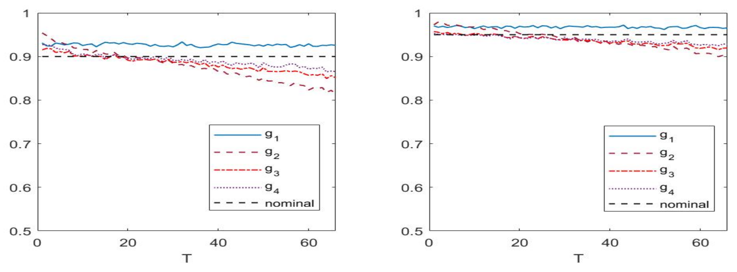
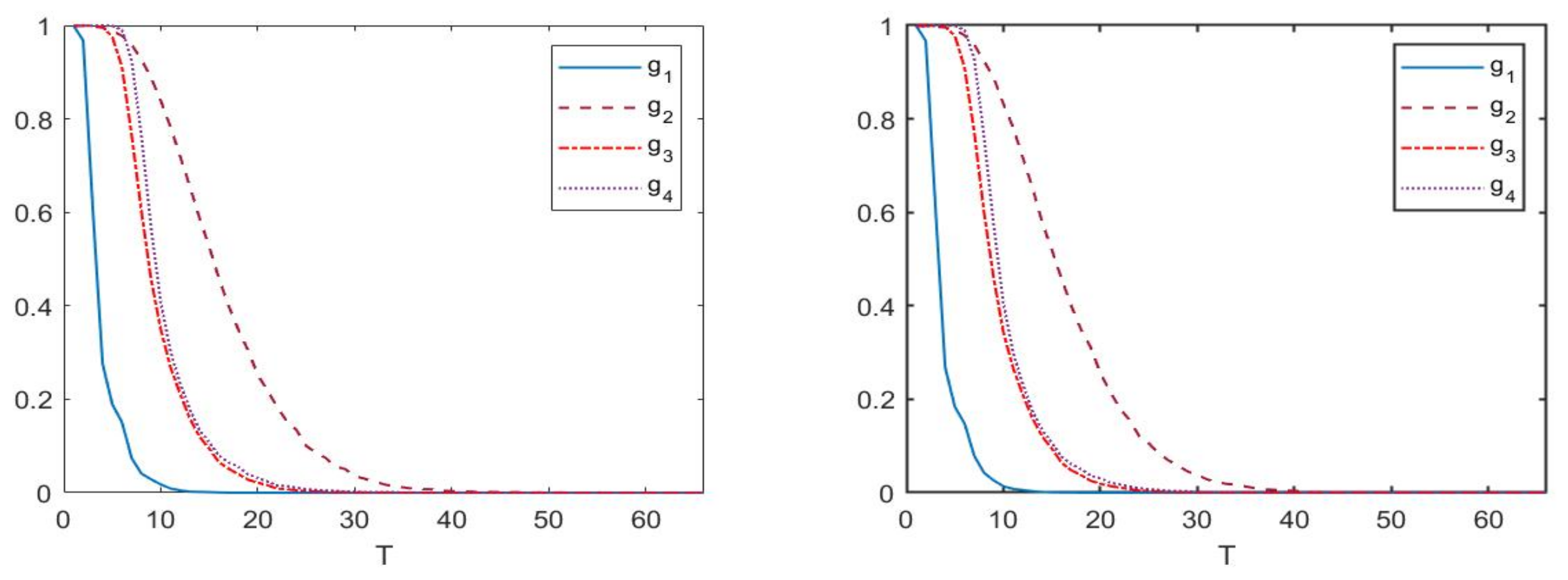
We computed the finite sample size and power for all cases. The results from the Monte Carlo, which is based on 10,000 replications, are reported in two tables (

Table 2. Coverage rates of the test statistics under ${\mathrm{H}}_0$.

T	$\mathit{\alpha }=0.05$					$\mathit{\alpha }=0.1$
	${\mathcal{W}}_{\mathbf{n}}$	${\mathcal{S}}_{\mathbf{n}}$	${\mathcal{U}}_{\mathbf{n}}$	${\mathcal{V}}_{\mathbf{n}}$		${\mathcal{W}}_{\mathbf{n}}$	${\mathcal{S}}_{\mathbf{n}}$	${\mathcal{U}}_{\mathbf{n}}$	${\mathcal{V}}_{\mathbf{n}}$
1	0.9746	0.9758	0.9554	0.9504		0.9331	0.9552	0.9144	0.9257
5	0.9691	0.9728	0.9536	0.9528		0.9304	0.9326	0.9107	0.9163
10	0.9683	0.9697	0.9499	0.9483		0.9289	0.9196	0.9044	0.9056
15	0.9671	0.9566	0.9443	0.9413		0.9270	0.9086	0.8995	0.9045
20	0.9671	0.9553	0.9459	0.9434		0.9261	0.9039	0.8952	0.8969
22	0.9665	0.9538	0.9456	0.9451		0.9242	0.8937	0.8925	0.8951
44	0.9662	0.9289	0.9320	0.9329		0.9234	0.8590	0.8758	0.8849
66	0.9643	0.8969	0.9172	0.9245		0.9218	0.8253	0.8591	0.8733

and

Table 3. Coverage rates of the test statistics under ${\mathrm{H}}_1$.

T	$\mathit{\alpha }=0.05$					$\mathit{\alpha }=0.1$
	${\mathcal{W}}_{\mathbf{n}}$	${\mathcal{S}}_{\mathbf{n}}$	${\mathcal{U}}_{\mathbf{n}}$	${\mathcal{V}}_{\mathbf{n}}$		${\mathcal{W}}_{\mathbf{n}}$	${\mathcal{S}}_{\mathbf{n}}$	${\mathcal{U}}_{\mathbf{n}}$	${\mathcal{V}}_{\mathbf{n}}$
1	0.9995	0.9996	0.9974	0.9968		0.9864	0.9969	0.9959	0.9959
5	0.1914	0.9887	0.9771	0.9993		0.1234	0.9242	0.7083	0.8737
10	0.0154	0.8420	0.3552	0.4170		0.0056	0.5565	0.1416	0.1478
15	0.0006	0.5225	0.0905	0.1040		0.0002	0.2365	0.0298	0.0376
20	0	0.2599	0.0185	0.0282		0	0.0881	0.0039	0.0091
22	0	0.1853	0.0093	0.0167		0	0.0573	0.0030	0.0057
44	0	0.0015	0	0		0	0	0	0.0001
66	0	0	0	0		0	0	0	0

) and two figures (Figure 1 and Figure 2). Table 2 and Figure 1 display the finite sample size and Table 3 and Figure 2 exhibit the finite sample power, respectively.

From Table 2, we see that the test statistic ${\mathcal{W}}_n$ performs stably relatively, with the length of time interval, T. The coverage rates of other three test statistics tend to decrease more clearly when T increases. Figure 1 shows the same results pictorially. This is consistent with our theoretical results, noting that Theorem 1 and Corollary 1 indicate that $K_n$ (hence T) cannot be too large, to guarantee a valid converge rate under the null hypothesis ${\mathrm{H}}_0$. Table 3 shows that all four test statistics tend to perform better uniformly when the time interval becomes longer under the alternative hypothesis ${\mathrm{H}}_1$, which is also consistent with our theoretical result. In fact, the only condition to assure the test statistics tending to infinity under alternative hypothesis ${\mathrm{H}}_1$ is letting $T\to \infty$. Therefore, an ideal choice for the length of the test period should be determined via a tradeoff between the size and power. To perform this, we computed the averaged errors of sizes and powers, namely, the difference between finite sample coverage rate and asymptotic coverage rate, of the four test statistics. The simulation results indicate that, for the high-frequency data with sampling frequency of five minutes, the best choice for the time interval of the test is between a month and two months.

5. Real Data Analysis

In this section, we implement the proposed test procedures to a real high-frequency financial dataset. The dataset consists of 5-minute close prices of the SP500 index from 1997 to 2000. To clear the data, we firstly removed the largest 3% returns to avoid the possible presence of jumps and no further adjustment was conducted for the data set. Finally, we obtained a total of 250,669 data points. We computed the test statistics with several periods, namely, a day, a week, a month, a quarter, half a year and a year, respectively. More precisely, for example, for the daily test, we took $n=78$ (n = 390, 1716, 5418, 10,296 and 20,592 for the weekly test, monthly test, quarterly test, semiannual test and annual test, respectively.) and $m_n=k_n=\lfloor \sqrt{n}\rfloor$, using the following statistic with $K_n=\lfloor n/m\rfloor$:

$${\mathcal{T}}_n:=\frac{1}{\sqrt{{\nu }_g{K}_n}}\sum _{k=1}^{K_n}\left[g\left(T_n^{\left(k\right)}\right)-{\rho }_g\right],T_n^{\left(k\right)}=\frac{{\sum }_{i=1}^n{\left({\Delta }_i^{n}X\right)}^3-3{\Delta }_n{\sum }_{i=1}^n{\widehat{\sigma }}_{(i-1){\Delta }_n}^2{\Delta }_i^{n}X}{\sqrt{\frac{2}{5}{\sum }_{i=1}^n{\left({\Delta }_i^{n}X\right)}^6}}$$

(18)

where we used the similar test function g used in the simulation.

Table 4. Rejection rate of tests.

Time Span	Nominal Level	${\mathcal{T}}_{\mathit{n}}$	${\mathcal{S}}_{\mathit{n}}$	${\mathcal{U}}_{\mathit{n}}$	${\mathcal{V}}_{\mathit{n}}$
Day	0.05	0.98	0.92	0.89	0.68
	0.1	0.98	0.90	0.87	0.57
Week	0.05	1	1	1	1
	0.1	1	1	1	1
Month	0.05	1	1	1	1
	0.1	1	1	1	1
Quarter	0.05	1	1	1	1
	0.1	1	1	1	1
Half year	0.05	1	1	1	1
	0.1	1	1	1	1
Year	0.05	1	1	1	1
	0.1	1	1	1	1

displays the values of the test statistics and related rejection rates of the tests based on these six different time spans.

From Table 4, for the time period longer than a day, all four test statistics reject the null hypothesis of the absence of the leverage effect. For the daily test, we see that ${\mathcal{T}}_n$ shows the highest rejection rate for all kinds of time periods, followed by ${\mathcal{S}}_n$ and ${\mathcal{U}}_n$; ${\mathcal{V}}_n$ has a lowest rejection rate. This is same as the order of empirical powers in the simulation study; hence, we may conclude that the leverage effect is a necessary component in modelling the high-frequency data of the SP500 index.

6. Discussion

In the current paper, we did not consider the common stylised facts of the high-frequency data, such that the jumps and microstructure noise. Here, we give some possible ways to deal with the effects of the jumps and microstructure noise. The process X contains jumps when, namely,

$$d{X}_t=b_{t}dt+{\sigma }_{t}d{W}_t+{\delta }_{t}d{J}_t,$$

(19)

where J is a pure jump process. In this case, one possible way to remove the effect of the jump is to use the threshold technique proposed by Mancini [23]:

$$\begin{array}{c}\hfill n\sum _{i=1}^n{\left({\Delta }_i^{n}X\right)}^3{\mathbf{1}}_{\{|{\Delta }_i^n|\le \alpha {\Delta }_n^{\varpi }\}}{\to }^{\mathcal{S}}3{\int }_0^T{L}_s{\sigma }_s^{2}ds+3{\int }_0^T{\sigma }_s^{2}d{X}_s+\sqrt{6}{\int }_0^T{|{\sigma }_s|}^{3}d{\tilde{W}}_s,\end{array}$$

(20)

where $\varpi <1/2$ is a positive integer. Then, the theory established in this paper should be extended to the case with jumps. For microstructure noise, we may try some de-noising approaches, such as the pre-averaging method proposed in Jacod et al. [24] or the realized kernel method suggested by Barndorff-Nielsen et al. [25] to reduce the level of microstructure noise and then use the idea in this paper to construct a test statistic to test the presence of the leverage effect. The other direction concerns the future implications of the results obtained in this paper. As implied by the results of the empirical study in this paper, the leverage effect is a necessary feature of high-frequency modelling; therefore, we may consider how to use the leverage effect to improve the usefulness of high-frequency data; for instance, we may add the leverage effect as a factor in predictive models predicting volatility and asset price, such as in the HAR model, etc.

7. Conclusions

In this paper, we propose a class of test statistics to test the presence of the leverage effect in modelling high-frequency data in financial markets. The test procedure is valid under shrinking sampling intervals. In real application, it proved a valid and reasonable test approach for the presence of the leverage effect within a moderately long time span, from a week to a quarter, for instance. Widely simulated studies further confirmed the performance of the proposed test statistics. The proposed test method was also applied to a dataset of the SP500 index; the result shows that the leverage effect is a necessary factor when the time span is longer than a week.

Some limitations of the present study remain. The first one is that the jump is not incorporated into the current setting, and the second is that the test is not robust in the possible presence of microstructure noise. We listed some possible ways to deal with these two issues in the last section. In view of the importance of both jumps and microstructure noise in financial high-frequency data, the extension of the current research in this direction deserves a future investigation.

References

- Ang, A.; Chen, J. Asymmetric correlation of equity portfolios. J. Financ. Econ. 2002, 63, 443–494. [Google Scholar] [CrossRef]
- Black, F. Studies in stock price volatility changes. In Proceedings of the 1976 Meeting of the Business and Economic Statistics Section; American Statistical Association: Washington, DC, USA, 1976; pp. 177–181. [Google Scholar]
- Christie, A. The stochastic behavior of common stock variances-Value, leverage, and interest rate effects. J. Financ. Econ. 1982, 10, 407–432. [Google Scholar] [CrossRef]
- Modigliani, F.; Miller, M. The cost of capital, corportation fiance, and the theory of investment. Am. Econ. Rev. 1958, 48, 261–297. [Google Scholar]
- Hens, T.; Steude, S. The leverage effect without leverage. Financ. Res. Lett. 2009, 6, 83–94. [Google Scholar] [CrossRef]
- Hasanhodzic, J.; Lo, A. Black’s Leverage Effect is Not Due to Leverage; Working Paper. Available online: http://ssrn.com/abstract=1762363 (accessed on 21 June 2022).
- Aït-Sahalia, Y.; Fan, J.; Li, Y. The Leverage Effect Puzzle: Disentangling Sources of Bias at High Frequency. J. Financ. Econ. 2013, 109, 224–249. [Google Scholar] [CrossRef] [Green Version]
- Wang, D.; Mykland, P. The Estimation of Leverage Effect With High-Frequency Data. J. Am. Stat. Assoc. 2014, 109, 197–215. [Google Scholar] [CrossRef]
- Aït-Sahalia, Y.; Fan, J.; Laeven, R.; Wang, D.; Yang, X. The Estimation of Continuous and Discontinuous Leverage Effects. J. Am. Stat. Assoc. 2017, 112, 1744–1758. [Google Scholar] [CrossRef] [PubMed]
- Kalnina, I.; Xiu, D. Nonparametric Estimation of the Leverage Effect: A Trade-off between Robustness and Efficiency. J. Am. Stat. Assoc. 2017, 112, 384–396. [Google Scholar] [CrossRef] [Green Version]
- Kinnebrock, S.; Podolskij, M. A note on the central limit theorem for bipower variation of general functions. Stoch. Process. Their Appl. 2008, 118, 1056–1070. [Google Scholar] [CrossRef] [Green Version]
- Delbaen, F.; Schachermayer, W. A general version of the fundamental theorem of asset pricing. Math. Ann. 1994, 300, 463–520. [Google Scholar] [CrossRef]
- Delbaen, F.; Schachermayer, W. The existence of absolutely continuous local martingale measures. Ann. Appl. Probab. 1995, 5, 926–945. [Google Scholar] [CrossRef]
- Delbaen, F.; Schachermayer, W. The Fundamental Theorem of Asset Pricing For Unbounded Stochastic Processes. Math. Ann. 1998, 312, 215–250. [Google Scholar] [CrossRef] [Green Version]
- Stojkoski, V.; Jolakoski, P.; Pal, A.; Ljupco Kocarev, T.S.; Metzle, R. Income inequality and mobility in geometric Brownian motion with stochastic resetting: Theoretical results and empirical evidence of non-ergodicity. Philos. Trans. R. Soc. A. 2022, 380, 20210157. [Google Scholar] [CrossRef] [PubMed]
- Zheng, C.; Wang, L. Option Pricing under the Subordinated Market Models. Discret. Dyn. Nat. Soc. 2022, 2022, 6213803. [Google Scholar]
- Bouchaud, J.P.; Potters, M. Theory of Financial Risk and Derivative Pricing: From Statistical Physics to Risk Management; Cambridge University Press: Cambridge, UK, 2003. [Google Scholar]
- Fouque, J.P.; Papanicolaou, G.; Sircar, K.R. Derivatives in Financial Markets with Stochastic Volatility; Cambridge University Press: Cambridge, UK, 2000. [Google Scholar]
- Renyi, A. On Stable Sequences of Events. Sankhya Indian J. Stat. Ser. A 1963, 25, 293–302. [Google Scholar]
- Aldous, D.; Eagleson, G.K. On mixing and stability of limit theorems. Ann. Probab. 1978, 6, 325–331. [Google Scholar] [CrossRef]
- Jacod, J.; Shiryayev, A.V. Limit Theorems for Stochastic Processes; Springer: New York, NY, USA, 2003. [Google Scholar]
- Andersen, T.G.; Bollerslev, T.; Diebold, F.; Wu, J. Realized beta: Persistence and Predictability. In Econometric Analysis of Financial and Economic Time Series; Fomby, T., Terrell, D., Eds.; Emerald Group Publishing Limited: Bingley, UK, 2006; Volume B, pp. 1–40. [Google Scholar]
- Mancini, C. Nonparametric threshold estimation for models with stochastic diffusion coefficient and jumps. Scand. J. Stat. 2009, 36, 270–296. [Google Scholar] [CrossRef]
- Jacod, J.; Li, Y.; Mykland, P.; Podolskij, M.; Vetter, M. Microstructure noise in the continuous case: The pre-averaging approach. Stoch. Process. Their Appl. 2009, 119, 2249–2276. [Google Scholar] [CrossRef] [Green Version]
- Barndorff-Nielsen, O.E.; Hansen, P.R.; Lunde, A.; Shephard, N. Designing realised kernels to measure the ex-post variation of equity prices in the presence of noise. Econometrica 2008, 76, 1481–1536. [Google Scholar] [CrossRef] [Green Version]
- Jacod, J.; Protter, P. Discretization of Processes; Springer: New York, NY, USA, 2012. [Google Scholar]
Figure 1.
The converge rates of five test statistics under , against the length of time interval T. (Left): a 90% nominal level. (Right): a 95% nominal level.
Figure 2.