Queueing Theory-Based Mathematical Models Applied to Enterprise Organization and Industrial Production Optimization

Abstract

In the paper, a new method was presented using queueing theory models in order to ensure an optimal production department size, optimized production costs and optimal provision. Queueing/waiting mathematical models represent the development matrix for an experimental algorithm and implicitly numerical approach, both successfully applied (and confirmed in practice) in a production section design for a real industrial engineering unit with discussed method technological flow and equipment schemes compatibility. The total costs for a queueing system with S servers depend on the number of servers. The problem of minimizing cost in terms of S was the main aim of the paper. In order to solve it, we estimated all the variables of the system that influence the cost using the Monte Carlo method. For a Jackson queueing network, the involved linear system has good properties such that it can be solved by iterative methods such as Jacobi and Gauss–Seidel.

1. Introduction

This paper aimed to achieve a simulation in terms of technological times of the operation of a Technological Fabrication System (TFS) and, based on it, created a methodology and an adequate optimization program, which takes into account the real behavior of the technological system to different production tasks.

The opportunity of this approach lies in the results and findings presented in several treaties and studies [1,2], which highlight that in the field of machine building, the share of technological time in manufacturing processes represents most of the time required. By starting from these observations, it can be said that there are enough resources and motivations in this respect for the development of research in this field that can be part of all the research regarding the optimization of manufacturing technologies.

Moreover, there is a unanimous appreciation that, unlike other time components on which there are several ways and ways of optimization, the field of technological time is relatively complex, and the optimization paths are insufficiently explored.

The tools used in this analysis are based on some mathematical devices provided by the methods of operational research, namely those related to the theory of expectation, adapted for simulating the operation in time of the TFS and thus modeled to allow the optimization of their dimensioning corresponding to variable production tasks. The application of queueing theory has seen spectacular development in recent decades, especially due to the various applications that this theory can solve. The foundations of this theory are found in numerous works, and the various specific aspects it can address are presented in the literature [3,4,5,6,7].

In Ref. [8], several queueing systems with one server are presented, namely Poisson arrivals and exponential services, Poisson arrivals and general (including the particular deterministic and above-mentioned exponential cases), and general arrivals and services. The case of S = 1 or even S > 1 servers is for exponential services per server and general (including Poisson and deterministic cases) services. In this paper, we studied the total cost for given arrivals (distribution and parameters) and the parameter of the exponential service time/server. Classical Jackson (with particular cases of series and parallel networks) and Gordon and Newell queueing networks are also presented [5]. The linear system that solves a Jackson queueing network is solved by the Gauss–Seidel method in this paper. With our C++ program for Jackson queueing networks, we read the number of nodes from the keyboard. We read the transition matrix (the probabilities that after finishing service in node i go to node j/living network) and the average number of arrivals/time units for each node from a text file. With these data, we computed the matrix and the right sides for the involved linear system, which we solved using the mentioned Gauss–Seidel method.

Certain methods proposed by queueing theory have gained enormous popularity in recent years. They use classic models adapted to the situations that appeared in practice. A three-dimensional Markov stochastic model over time, with two service phases, is presented in [9]. The matrix-geometric solution method and the Gauss–Seidel iterative method based on observable waiting rules were used. This gives major indicators for the system, such as the average length of stay and the expected duration of the requesting nodes. Numerical examples prove the validity of the models used. Finally, the benefit function offers the optimal social parameters.

At the moment, queuing has become a common phenomenon in various stages of production systems. This reduces the time required for managers and manufacturers to complete the desired task. As a result, the mathematical theory has become an indispensable tool for analyzing various practical situations. Numerical methods are always basic tools for applying these methods [9,10].

One of the possible applications of Queuing Theory is the optimization of service capacity. It is considered a hypothetical situation in which a company operates m machines, and the intervals between failures and repair times are distributed exponentially. Damaged cars are repaired by n repairers (n < m). A mathematical model of the problem for optimizing the number of repairers in relation to system costs is presented in [11]. Research that aims to determine better solutions for workspaces in an enterprise with many machines is presented in [12]. Numerous works deal with problems of optimization of production processes [13,14,15,16,17,18,19,20,21].

We also noticed that the linear system involved in solving a Jackson queueing network is diagonally dominant because the coefficient A_ii is one and the other values are probabilities. Therefore this linear system can be solved by the Gauss–Seidel method, as we performed in this paper.

The classical approach for the queueing systems with general arrivals, exponential services and S servers is first to determine [8] the ratio of the geometric distribution of the number of units in the queue. Next, we determined the ratios between the probabilities of having $0<n\le S$ working servers and no working servers and, from here, the probability of no unit in the system. Next, all elements were computed. The difficulty of computing p₀ (as working time) led us to use Monte Carlo methods (presented in [22]) to estimate first the number of units in the system/in the queue and compute all the other elements as in this paper.

In the paper, the authors applied (in the context presented before) the theory and mathematical models of expectation in the industry and developed a new method of optimizing a production section in terms of sizing in accordance with variable production tasks. The mathematical model and the programs made by the authors based on it were verified in practice on an existing enterprise in the machine building industry described in the case study.

2. Simulation and Optimization of TFS Operation, Based on Waiting Theory

The study of the mathematical models of expectation is based on the methods of probability theory and mathematical statistics, and the purpose of this study in the technological field is to determine the effective solutions for organizing a manufacturing process—including the TFS sizing—taking into account the real elements that influence this efficiency.

In our consideration the following definitions are used:

Unity = an element of the crowd to be “served”, e.g., the part to be processed at a machine tool;

The station = the point where the "serving" is performed (machine tool, processing center or by a global name, TFS);

Waiting string (thread) = the set of units waiting to be served without the unit that is served;

Calling system = includes the set of units in the process of serving;

Input flow = characterizes the way in which the units enter the system;

The output flow = characterizes the way in which the units leave the system;

The serving time = effective duration required for serving (processing the part);

Waiting time = waiting time before serving.

We specified that the effect of mathematical modeling and of the software realized within the work goes beyond the context/objectives related to the optimization of the specific dimensioning/endowment of the enterprise and enters the subsidiary in an area of interest and “fashionable” at the moment, namely, in the one related to the zero manufacturing defect concept (ZDM [23,24]).

The simulation was achieved by modeling the calling wires in the technological systems with one or more workstations—assimilated as “serving stations”. The optimization of the technological systems for this case is based on the existence of two contradictory tendencies—one of oversizing to reduce the costs of waiting, and the other of under-sizing to reduce the costs of the systems—within this chapter being realized as a methodology, algorithm and program adequate to the analysis of the behavior and optimization of the respective systems.

Due to these two contrary trends, there is the possibility of optimizing the technological system as a whole by stimulating its functioning; the path was chosen within the subchapter, developed on the basis of calling models. From this point of view, we considered that the main problem of applying the theory of waiting in the mentioned field consists in establishing and justifying the material expenses necessary to achieve a certain level of quality of service in the waiting phenomena.

It is true that, as is known, this relatively new concept related to quality and sustainability is the latest approach to improving quality and is based on four strategies of detection, prediction, repair, and prevention, seemingly different from the strategy presented in our paper.

In general, in the technique and in the technological management, the “serving” problems (in this notion including the different requests to which the analyzed system is subjected) are more promptly realized the higher the capacity of the system. In practice, however, one cannot resort to the exaggerated expansion of the capacities (for the technological manufacturing systems, these being the power and the gauge of the machines), because this would also imply the unjustified increase in their costs. If, as it happens in the general case, the duration of “servings” is different from unit to unit, then we say that it is random.

The literature [2,25,26] indicates the existence of several types of queueing/waiting systems with uses in different fields (transport, telecommunications, etc.) many of them can also have applicability in the industrial field through adequate modeling.

A generalization of the above series and parallel queueing networks is the Jackson queueing network. We have n nodes in the network with Poisson arrivals of parameter ${\lambda }_i$ and the service exponential with parameter ${\mu }_i$. After finishing the service in the node i, the customers go to the node j next, with the probability p_ij, or leave the network with the probability p_i0. The condition for a Jackson Network (Garzia et al., 1990, [27]) is that each node is on a path from input flow and leaving the network. It is proven that for a Jackson network, each node is independent, and it acts as if the arrivals are Poisson of parameter ${\Lambda }_i$ is the solution of the linear system:

$${\Lambda }_i={\lambda }_i+{\displaystyle \sum _{j=1}^n{p}_{ji}\ast {\Lambda }_j}$$

(1)

The above system cannot changed because it is the formula for Jacobi/Gauss–Seidel method. A series network is a particular Jackson queueing network with p_ij = 1 for each node except the last, with p_i0 = 1. The parallel network is the particular Jackson queueing network with p_i0 = 1 or $p_{ij}=\frac{1}{N_i}$, where N_i is the number of successors of the node i. There is a possibility of having $p_{ij}=\frac{1}{N_i+1}$, making possible living the network from each node. In [6,7], a method to solve the system was presented (1) by simulation of the corresponding Jackson queueing network, with ${\mu }_i$ large enough to avoid locking node i. The average number of units in the node i is estimated as $\frac{{\Lambda }_i}{{\Lambda }_i+{\mu }_i}$.

The waiting models are analyzed in specialized papers in the field of mathematics, e.g., [2], but other specialized treatises with applications in the technical field [2,26,28] are also classified according to the input flows as follows:

(a)

Models with determined input flow (D), at which the units arrive at regular intervals t₀. The function of allocating the number of units that enter the system is:

$$P\left(t\right)=\{\begin{array}{c}1 for t\ge t_0\\ 0 for t<t_0\end{array} ;$$

(2)

(b)

Models with random input flow or (poissonian) P,—if the units arrive after the Poisson distribution of parameter a where a is the average of inputs in a range Δt reference.

The number of units entered in the range [0, t] has the Poisson distribution:

$$P_n\left(t\right)=\frac{{\left(at\right)}^n{e}^{-at}}{n!}.$$

(3)

(c)

Models with Erlang input flow (E_K), to which the function of distribution of the number of units entering the system is:

$$P_K\left(t\right)=\frac{{\left(K/m\right)}^K}{\left(K-1\right)!}{t}^{K-1}\cdot e\frac{-Kt}{m}.$$

(4)

(d)

Models with general independent input flow (GI) are used if there is no hypothesis on the F distribution function except for the existence of the average value m > 0.

In [8], the following classification of waiting models is provided:

(a)

The models with Poisson input flow and exponential service, one server/S server, finite population/infinite population. The model with a finite waiting room is also treated, where if a customer finds on arrival K other customers in the system, they survive the system. In this way, most K units are in the system;

(b)

The models with Poisson arrivals, general services and one server. The expected number of units arrived in the system (the parameter of Poisson distribution), a, and the probability distribution of services, b(t) are given. The queue is not bordered. All the elements are computed in terms of the parameter a and the moments’ generating function of services (Laplace transform of b) as follows ([8]);

(c)

Models with general input flow, exponential services and S servers. The parameters of the model are the number of servers, the parameter of exponential service u, and the probability distribution function a of inter-arrival times, a;

(d)

Models with general input, general service and one server are also treated in [8]. There are considered the moments’ generating function for both arrivals and services and the decomposition in simple fractions of A^∗ and B^∗, and all the elements are determined by using the pairs of terms.

The model with Poisson arrivals, general service and S servers is the generalization of the above model (b) from the Kleinrock classification.

In [22,29], such model in the particular case pf PH(α,T) inter-arrival time was considered. A PH distribution is the distribution of the time that a continuous absorbing Markov chain is absorbed. α is the initial probability vector, and T is the transition probability (it becomes zero when the Markov Chain (see [28]) is absorbed).

A matrix Q is computed, and from equation Q^T∗x = 0, we determined x_i in terms of x₁. After this, we estimated the vector x as the vector of probability. The methodology is similar to the birth and death process in the case of Poisson arrivals and exponential services.

The discipline with an impatient customer is also considered. It is the classical FCFS discipline, but the customer waits in a waiting string for his impatient timer X, which is exponential of parameter ξ.

Another model with Poisson arrivals, general services and S servers was simulated in [25], considering the disciplines FCFS and RA = Random Assignment and previous process. Two models with switching to FCFS were also considered, one after a specific non-random time and the second after a random time is greater than a specific non-random time.

An algorithm in four steps is as follows: generating a model with only one server during a given period; simulating a process of making a queue empty; the third model with RA discipline; finally, combining the first and the third model. Therefore there were simulated three models: two forward and one (the second) backward.

In the above-considered models, the arrivals are independent and identically distributed, and the same for services. In [8], the $PP\infty :\left(\infty /FCFS\right)$ is the limit case for arbitrary arrivals, exponential services and S servers when $S\to \infty$ was presented.

In [30,31], for the above model, the arrivals were considered Hawkes processes. In fact, only the first arrival was Poisson, and the other arrivals were modified according to the history of inter-arrival moments t_i:

$$\mathsf{\Lambda }\left(t\right)={\lambda }_{\infty }+{\displaystyle \sum _{i=1}^{n-1}{B}_i\ast h\left(t-t_i\right)}.$$

(5)

where $\mathsf{\Lambda }\left(t\right)$ is the conditional intensity of the Poisson process, ${\lambda }_{\infty }$ is a constant, B_i are independent random variables and $h:[0,\infty )\to$$[0,\infty )$ is the excitation function.

A model with only one server when the services depend on arrivals through some types of copulas was presented in [6,9]. For comparison with the independence case, a model with Poisson arrivals and exponential services was considered as a case study.

In [22,32], multiple types of customers were considered, with Poisson arrivals of parameter p_i∗a, S servers and exp(u_i) service time for customers of type i. Constraints for the s servers were also considered. For instance, one server can use the classical FCFS discipline, while another server can use priorities. The GRAND = Gready RANDom discipline was used. It means that each arriving customer is randomly assigned to a server that can serve them uniformly. In another algorithm, GRAND(aZ), some occupied servers are also considered. For instance, between two servers with priority, sometimes an occupied server where the customer has higher priority is preferable to a free server where the customer has lower priority.

Classical Jackson (with particular cases of series and parallel networks) and Gordon and Newell queueing networks are also presented [27]. The linear system that solves a Jackson queueing network was solved by the Gauss–Seidel method in this paper.

By taking into account the findings resulting from several treatises, studies and experimental research were carried out on the analysis of the development of technological processes for different production tasks [26,27], i.e., it was estimated that in this field, the most appropriate waiting model to characterize, as faithfully as possible, the behavior in the time of the technological system of manufacturing at variable production tasks is the PPS model, with arrivals and servicing in the random system (Poissonian) and stationary waiting.

3. Method and Model

In this section, we considered an industrial PPS queueing system, and we solved the system as follows. First, we determined the formulae for the classical S = 1 model, Poisson arrivals and exponential services. Next, we optimized the total cost of the PPS queueing system, and we noticed (our contribution) that the cost increases for S greater than an upper limit. Our C++ program computed this limit, and for S lower, we simulated each system on a given period using the Monte Carlo method (the sum of generated times is greater than or equal to the period, and we stopped when this condition was fulfilled). We first estimated the expected number of units in the system/in the queue, and from there, the other elements and the total cost for each S.

By taking into account the behavior over time of a technological manufacturing system subjected to variable production loads, it was experimentally found [33] that the models that most accurately approximate the operation of the TFS are the Poissonian models. For mathematical modeling, in order to achieve an algorithm and an optimization methodology appropriate to the objectives presented within this chapter, we chose the model PP1:(∞/FCFS) as the basis.

It assumes the following hypotheses:

• Arrivals are random (Poissonian);
• The servings are all random, exponential;
• The system is with a single station;
• The size of the string is indeterminate;
• Serving discipline: first come, first served.

For the study of the behavior of this waiting system (understanding by this the system formed by the machine tool, landmarks in process, pending landmarks), the following notations were made (

Table 1. The list and significance of notations used.

Symbol	Significance	Unit Measure
$P_n\left(t\right)$	the probability of there being n units in the system at time t;	-
$P_0\left(t\right)$	the probability that there is no waiting in the system at the time t;	-
$P\left(t\right)$	probability of being waiting at time t;	-
ns	the average number of units (parts) present in the system;	-
nf	the average number of units present in the sequence of units;	-
ts	the average waiting time in the system;	min.
tf	the average waiting time in the row (thread);	min.
a	the average number of entries-arrivals-in the system in the unit of time;	pieces/min
u	the average number of servings per unit of time;	pieces/min
r	the average inactivity rate of the stations in the system;	-

):

Studying the waiting model proposed in order to achieve an optimization methodology involves completing the following steps:

(a)

Determining the law of distribution of the number of arrivals for the classical PPS queueing systems using the birth and death processes [34];

(b)

Determining the distribution of time between two successive arrivals.

Let us be the random variable X = the time between two arrivals. We considered the moment of arrival of the first unit as an initial moment. The following sizes were defined:

• $P\left(X>t\right)=P_0\left(t\right)=e^{-at}$—the probability that the time interval X between two arrivals is greater than t;
• $F\left(t\right)=1-e^{-at}$ = the distribution of time between two arrivals;
• $f\left(t\right)=F^{\prime }\left(t\right)=a{e}^{-at}$ = probability density. (Obviously $t\ge 0$).

If the average interval between two arrivals is inverse to the average number of arrivals in the time unit, the distribution of the time intervals between two consecutive arrivals is an exponential distribution with the average $\frac{1}{a}$.

Generalization: We took into account the waiting system as a whole (considering both the input and output flow of the parts to a machine tool).

Assumptions:

• At time t, there are n – 1 units; the interval Δt enters and exits a unit;
• At the time t, there are n units; Δt does not enter or exit any units;
• At the time t, there are n units and enter and exit into Δt, a unit;
• At the time t, there is n + 1, enter 0, and exit a unit in the same interval Δt.

The probabilities of input and exit, respectively, of a unit in the system in the interval Δt are: aΔt and uΔt, respectively. With these considerations, we obtained the probabilities $P_n\left(t\right)$ from the Kolmogorov–Feller equations for birth and death processes [35,36].

(c)

Determination of auxiliary parameters—from the above-mentioned birth and death processes and the Little theorem [35], we obtained PP1 queueing system:

$$\{\begin{array}{l}{\overline{n}}_s=\frac{r}{1-r}\hfill \\ {\overline{n}}_f=\frac{r}{1-r}-r=\frac{r^2}{1-r}\hfill \\ {\overline{t}}_s=\frac{1}{u-a}\hfill \\ {\overline{t}}_f=\frac{1}{u-a}-\frac{1}{u}\hfill \end{array}.$$

(6)

The following conclusions were made by taking into account the results obtained from this analysis and the attributions made initially for adapting the theoretical model of waiting for the concrete case of a technological manufacturing system:

1. If a > u, the arrival flow is superior to the serving one and the waiting thread increases unlimitedly, which means that at TFS, respectively, the parts accumulate in order to be processed continuously; the respective work becomes a “narrow point”;

2. If a = u and P = 1, the number of pieces that enter the waiting thread will also increase continuously, as it results from the expression of nf at which the denominator descends to zero;

3. If a < u, the waiting string has a finished length, and after a while, the manufacturing system enters the stationary regime, where it can be coordinated and optimized and can proceed to the realization and application of the optimization algorithm.

Note: The PP1:(∞/FCFS) studied model allows the analysis of the operation of a TFS subjected to variable production tasks independently and in compliance with the hypotheses presented regarding the character of arrivals, services, etc.

In this chapter, we aimed to study the behavior of TFSs, not only individually but also at the level of the manufacturing line, and we also wanted to achieve a methodology of global optimization in terms of the costs of waiting in the system. From the specialized literature [6,8], we used the specific relationships that characterize other Poissonian tunes models, apart from the basic one, with frequent applicability in the field; namely, the models PD1:(∞/FCFS), PP1:(M/FCFS) and PPS:(∞/FCFS).

In the literature, in papers [28,36], the waiting models with constant serving time for the general case of multiserver systems were developed in detail. Therefore, the expressions corresponding to the characteristic sizes of the PD1:(∞/FCFS) could be obtained immediately by customizing the number of stations to the unit value, and they are presented in module 2 of the general algorithm.

The optimization process involves determining the compromise between the cost of waiting and the cost of serving so that the expenses caused by the waiting phenomenon—which under the given conditions is inevitable—can be minimized.

As in the other optimization processes, the identification of a value as optimal is based on the existence of two contradictory tendencies, namely Figure 1:

We noticed that C_opt has a global minimum, and it is bimodal. After the minimum, we also noticed that after S_opt (optimal number of servers), the cost increased almost linearly. Ii oversizes the industrial system by increasing the number (S) of workstations—TFS—servers, which has the effect of increasing the production capacity, thus implicitly decreasing the waiting times for parts. Obviously, this causes a decreasing allure of the component. Cost of waiting parts = $C1\cdot a\cdot tf=C1\cdot nf\cdot T$, where:

• C1 = the cost of waiting for the part [lei/unit. Time];
• a = number of parts entered into the system in the unit of time;
• tf = the waiting time on the wire;
• nf = number of pieces in the waiting thread;
• T = unit of measurement of time (hour, min.).

At the same time, the increase in the number of servers causes an increase in the investment in fixed assets, which leads to an increase in costs that refer to—the stationing of the TFS, so an increasing allure of the component:

Cost of waiting TFS$=C2\cdot S\cdot (1-r)$, where:

• C2 = the cost of stationary the TFS [lei/unit.time];
• S = number of TFS;
• r = the rate of use of the TFS.

Similarly, it was demonstrated that the undersizing of the system leads to an increase in the costs related to waiting for the parts and, respectively, a decrease in the costs of stationary/waiting for the TFS.

From the composition of the two contradictory tendencies, it results—as is represented in Figure 1—that for a certain structural sizing of the system (S_opt), the total costs of waiting, Cs(i), are minimal.

$$Cs(i)=C1\cdot a\cdot tf+C2\cdot i\cdot (1-r)$$

(7)

where: i = 1 … S = number of workstations, stations, servers, TFS.

In order to facilitate the analysis of the waiting in the system, based on the following algorithm, a simulation program that would allow both the knowledge of the behavior of the industrial and technological system at different production tasks was developed within the work, as well as providing solutions regarding its optimal sizing—presented in the following. We first chose the model PP1, PPS or PD1, with the option of the finite population for PP1. For the PPS model, we optimized the cost as in this paper, using the Monte Carlo methods. The calculation algorithms are presented in Appendix A.

4. Case Study Regarding the Simulation and Optimization of TFS Operation Based on Waiting/Queueing Models

4.1. Case Study and Methodology for Manual Calculation of Parameters and Optimization of Waiting Systems

In carrying out these researches, we started from the assumptions and premises imposed on the waiting models adapted to the technological manufacturing systems presented, to which we added an attribute necessary to achieve an analogy in real time of the behavior of the industrial system as a waiting system, namely the one regarding the serial character of the waiting models used.

Two specifications must be made: If we analyze the behavior of a technological system as a waiting system for the realization of a single operation that can be performed at any of the TFS pending, then the analysis is made based on the presented methodology. If the behavior of the industrial system of waiting for a succession of operations corresponding to a certain technological process is analyzed, then the chosen waiting model must be imposed a specific attribute related to the serial character of the system.

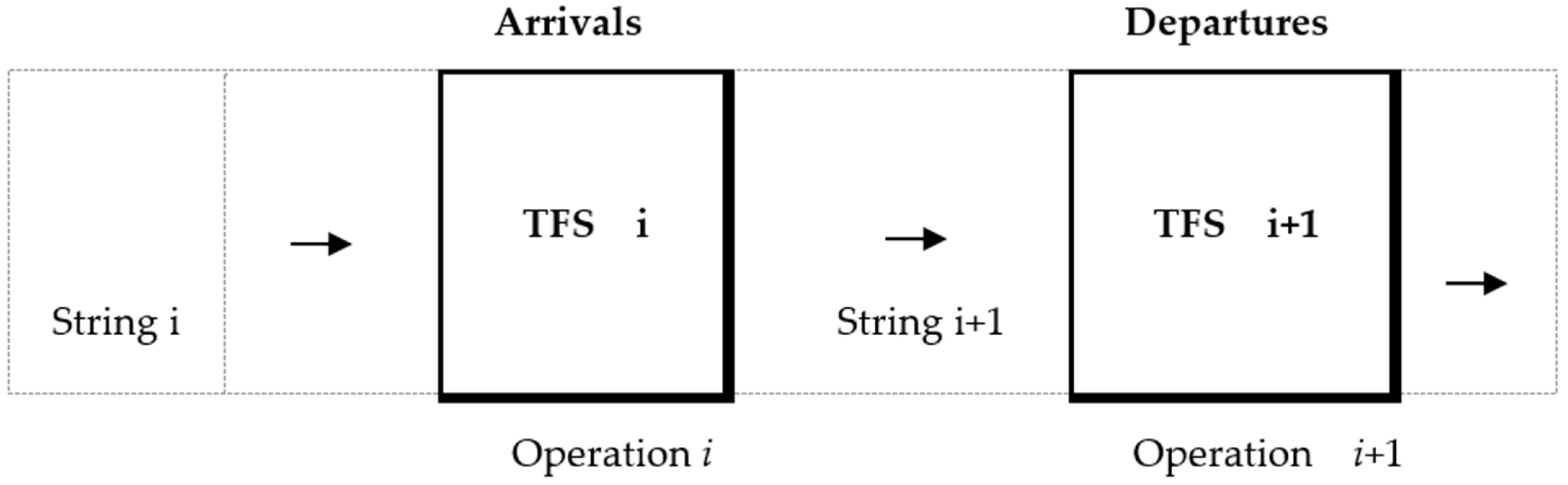
This feature takes into account the fact that, at flow-based processing, the outputs of a waiting process from a certain server (workstation TFS) are inputs for the next server (Figure 2), and it has relevance for the study of each waiting model in terms of the interaction between workstations and their influence on the behavior in time of the system.

In the following analyses, the approach was made in both ways in order to observe the behavior in terms of technological times of the industrial systems subjected to variable production tasks in a more faithful manner.

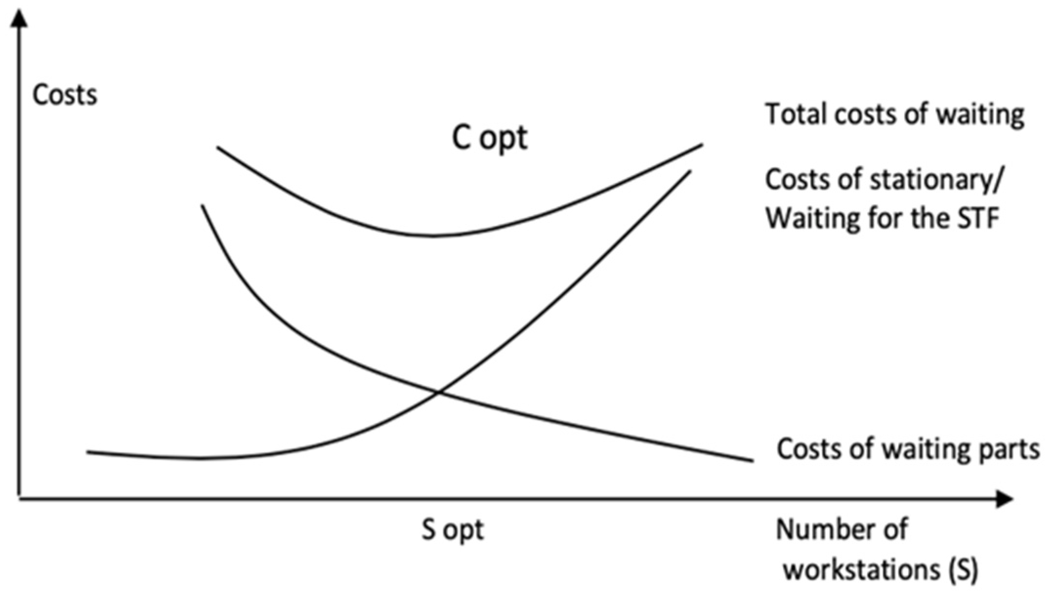
First, in the “manual” calculation, we took into account—for reasons related to space—a singular and significant example of a waiting system formed when processing a landmark in a production section, aiming that based on the parameters of the model, in the end, optimization of the system structure in terms of costs caused by waiting for parts, on the one hand, and waiting/stationing of servers, on the other hand, would be achieved. This involves determining the trade-off between the cost of waiting and serving. We proceeded through the following steps:

• Determining the period of time during which the system can be considered stationary;
• Timing of parameters a and u;
• Verification of the consistency test (${\chi }^2$);
• Calculation of waiting parametres— r,$P_n\left(t\right),\hspace{0.17em}{P}_0\left(t\right),\hspace{0.17em}{\overline{n}}_s,\hspace{0.17em}{\overline{n}}_f,\hspace{0.17em}{\overline{t}}_f,\hspace{0.17em}{\overline{t}}_s,\hspace{0.17em}\overline{r}$;
• Optimizing the total cost of waiting by taking into account the costs caused by waiting for the parts and servers in the system.

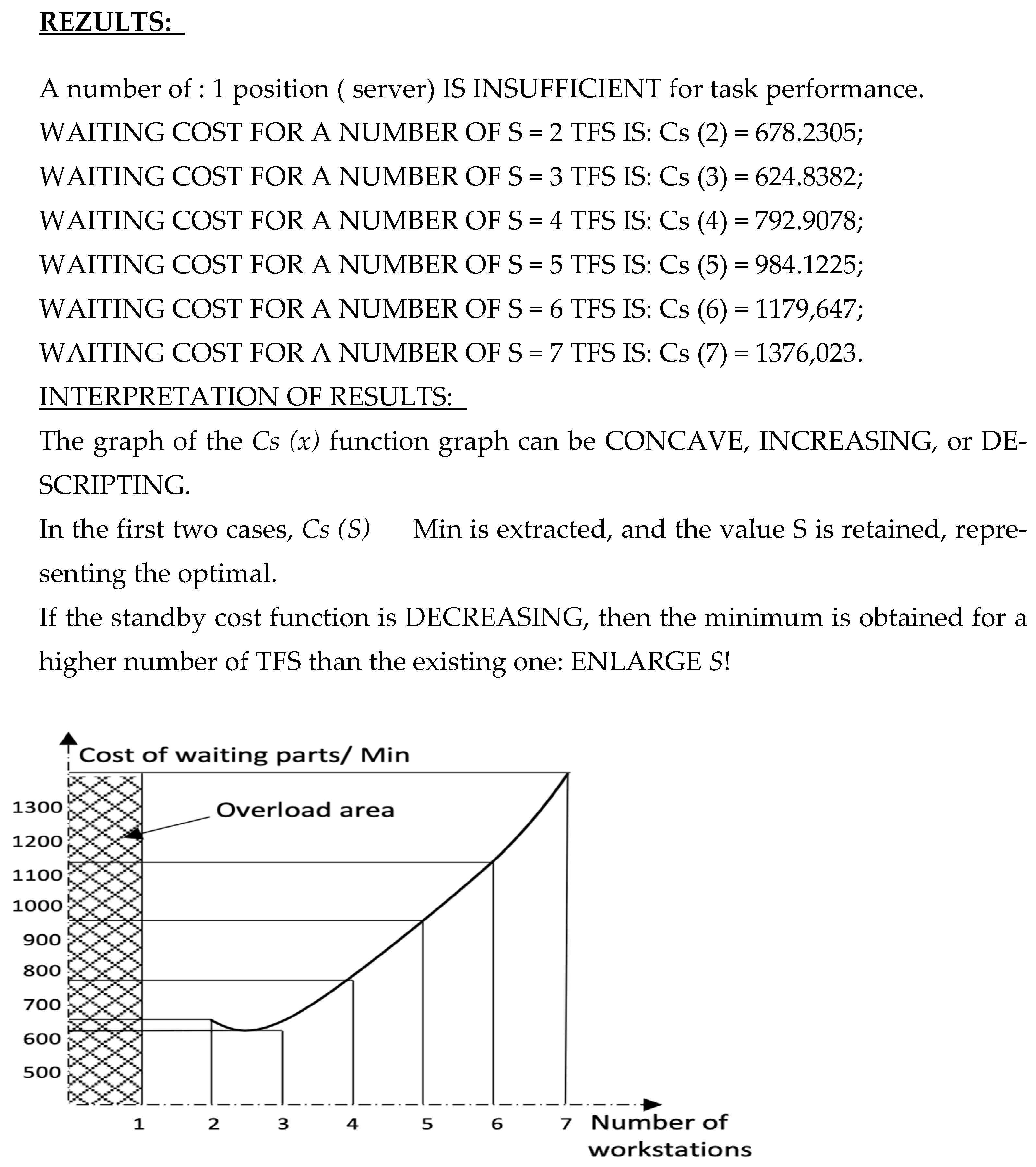
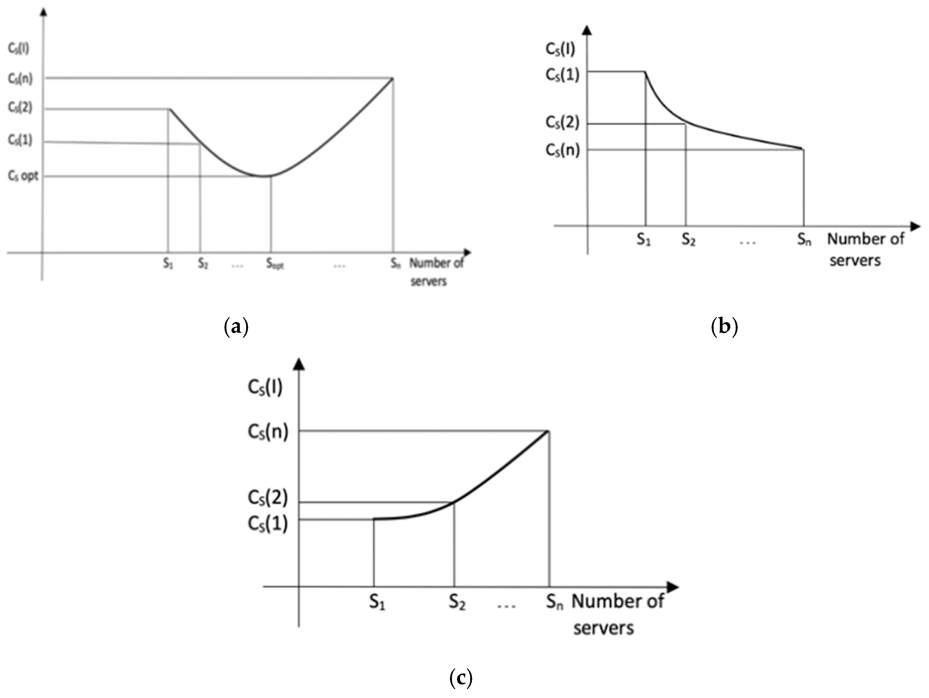
The objective was to identify the number of servers S_opt that minimizes the costs of waiting in the system C_s.

In the version of the “manual” calculation, it is necessary to individually calculate C_s (i) for different values i and values of S until the value i = S_opt corresponding to is found:

$$C_s{(i)}_{optim}=\underset{i\in N}{\min }\left\{\hspace{0.17em}\left[C_{1}a\hspace{0.17em}{\overline{t}}_f+C_2\cdot i\cdot \left(1-r\right)\right]\hspace{0.17em}T\right\}$$

(8)

As a characterization, the “manual” calculation method is somewhat laborious due to the modification of all the parameters of the waiting with the varying of i and the calculation based on the combinatorial analysis for i > 1, which is why, moreover, we also realized the methodology and the calculation program of assisted optimization of the parameters of the waiting system.

By returning (considered a server or serving station, such as the TFS used, whether it is a processing center or another machine tool, and the units under waiting) the semi-finished products (parts) to be processed, in order to decide if a second machine tool is needed to improve the serving or if its introduction into manufacture is uneconomic in the given situation, the waiting phenomenon and the overall costs related to it are studied.

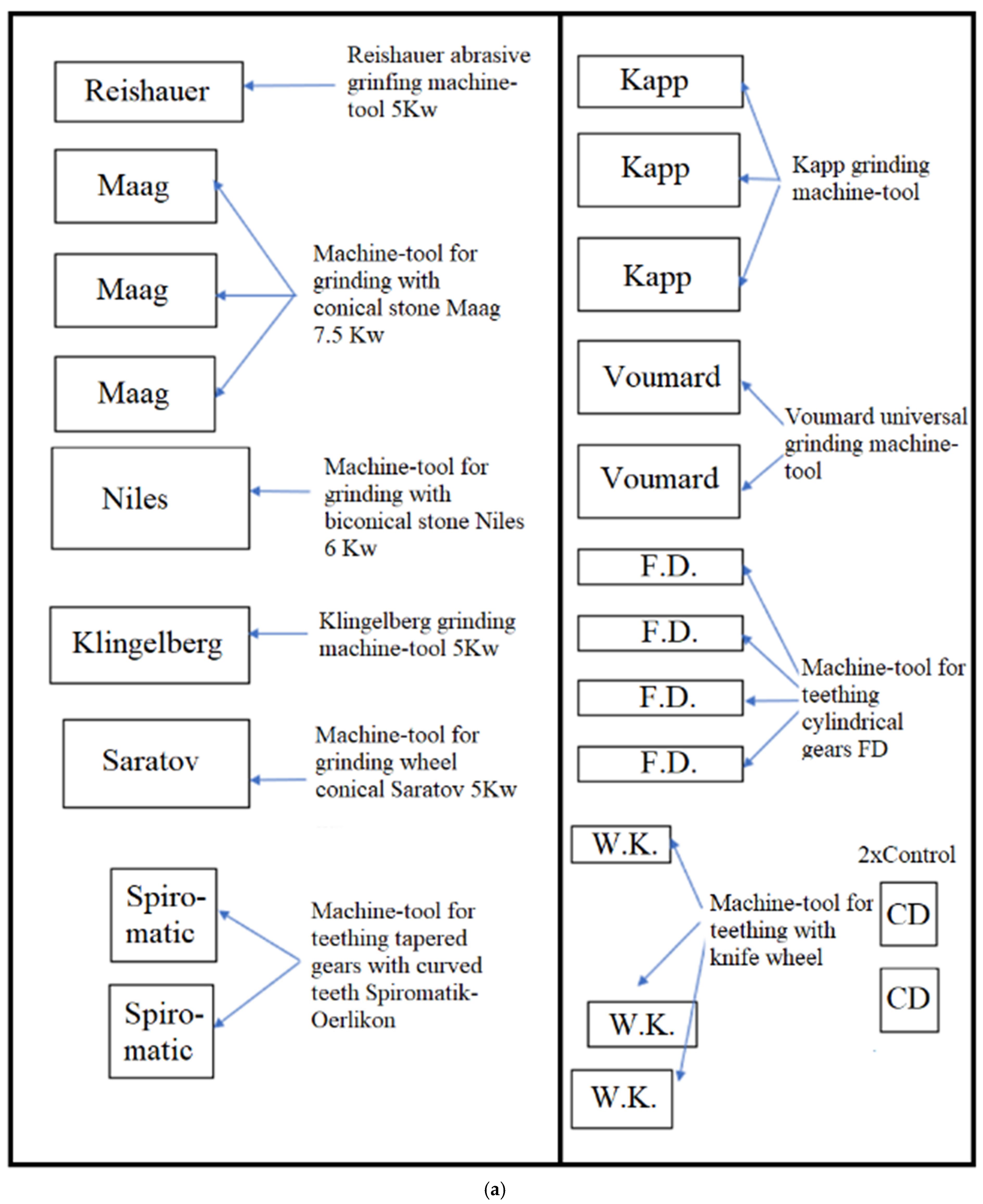
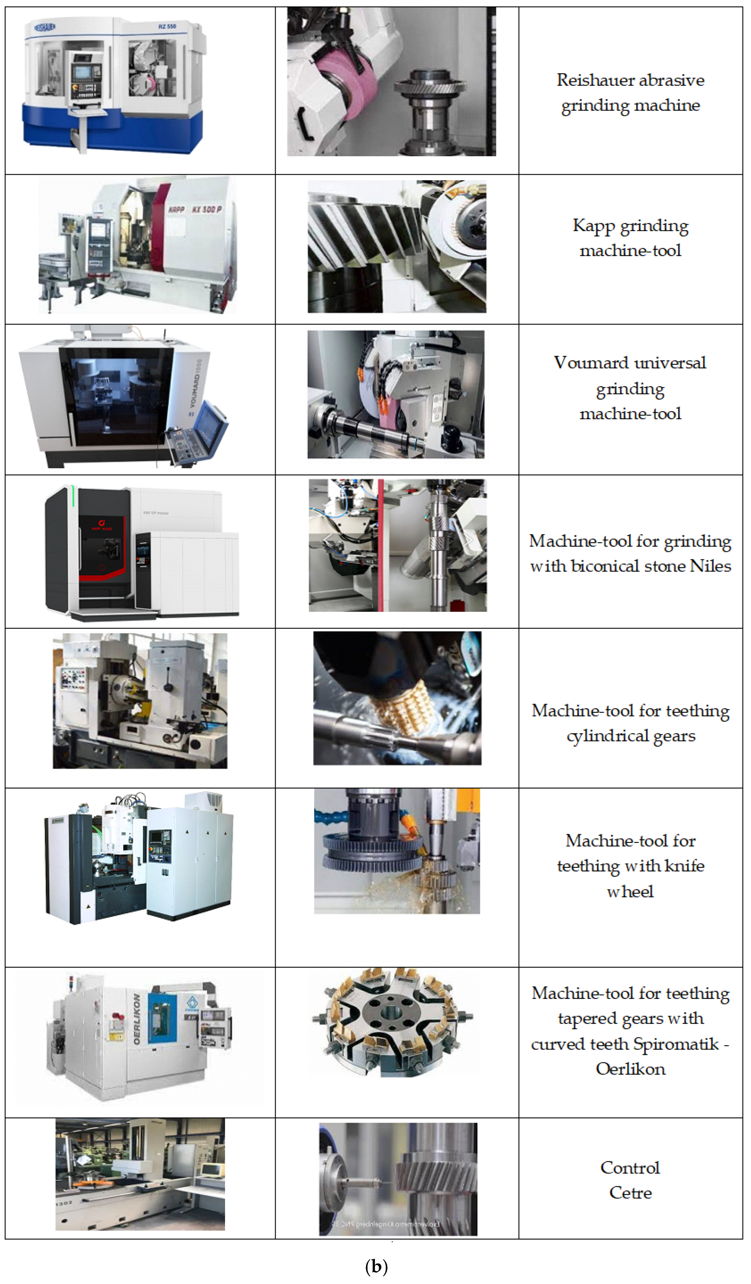
It analyzes the waiting phenomena that occur in a concrete processing case, such as the gears from the component of a horizontal machine for milling and boring, which are small series manufactured at a real factory along automatic lines (Figure 3a,b).

The fluctuation of orders, depending on the market requirements and implicitly the production load, from one period to another justifies the application of the waiting analysis. Observations are made on the process, and the stages I–V presented, necessary for optimization, were taken.

Stage I. involves establishing the assumed stationary periods in terms of waiting in the system. Then, it is assumed stationary the periods when the presence of the blank(s) pending is relatively high, and the waiting system relatively balanced. From observations made in time on the technological process of processing the analyzed group of gears, it was experimentally found that, except for a “weemble” interval of about 30 min, from the beginning of each exchange in which the number of pending parts is insignificant and varies according to indeterminate laws, in the rest of the working interval, the waiting process can be considered stationary. Generally, in most of the analyzed intervals, there is a super unit number of pending parts, another number of parts under processing, the volume of both categories influenced by the rate of entries, the service capacity of the industrial system, etc. We, therefore, considered that the period T for which the process becomes stationary is about 7.5 h or 450 min, and we then used the same unit of measurement in the analysis of waiting on the parameters.

Stage II. involves the determination based on the timing of the parameters a and u (where a is the average rate of inputs and u = the average rate of servings in the unit of time). It should be mentioned that, in order to respect the statistical character of the study v. [2], it is necessary that when the signification test is performed χ²,the number of elements of the crowd is greater than or equal to 50.

In our case, in order to cover the reference period, we formed the set of analysis from 75 intervals of 6 minutes for the study of arrivals, whether the intervals are consecutive or not.

With these experimental data, it is possible to calculate the average of the distribution of the arrival M(x), which is 1.17. Of the seven intervals, the last three of them had less than five values; thus, we only considered four intervals. The ${\chi }^2$ statistics is 0.508, while the ${\chi }_{2;0.1}^2=4.60517$. Therefore we accepted the hypothesis of Poisson distribution of 1.17 for 6 minutes, hence 0.19/min.

In parallel with this, for the study of the services, observations and timings were made on the actual duration of the services. Respecting the condition of choosing a large number of observed cases, at least 50, we choose a number of 75 serving cases—machined parts.

Because the servings were made in several intervals of the form $\left[t_1,\hspace{0.17em}{t}_2\right]$, we considered each range concentrated in its average value $\frac{t_2-t_1}{2}=\Delta t$.

We obtained the expected service time of 7.847, and the estimated parameter was u = 0.127. Because all the last five intervals out of nine had less than five values, we grouped them, obtaining five intervals. The ${\chi }^2$ statistic was 4.42818, while the quantile was ${\chi }_{3;0.1}^2=6.25139$. Therefore we accepted that the service are exponential with u = 0.127.

Stage III. According to the initial presentation, this consists in verifying the hypothesis that arrivals and services are Poissonian. The test was used for this purpose ${\chi }^2$ (see Appendix B,

Table A1. The results for S = 1.

r	Ns	Nf	Cost	p0	pS	pw
0.6	1.5	0.9	235	0.4	0.24	0.6
0.59319	1.63988	1.04669	258.706	0.40681	0.24132	0.59319

,

Table A2. The results for a maximum of 7 servers.

S	r[S]	Ns[S]	Nf[S]	Cost[S]	p0[S]	ps[S]	pw[S]
1	0.59114	1.54969	0.95856	291.569	0.40886	0.2417	0.5911
2	0.39915	0.95767	0.15937	298.3205	0.45117	0.1499	0.2495
3	0.28556	0.92647	0.06979	402.0285	0.47792	0.0687	0.0962
4	0.19698	0.79418	0.00625	496.4375	0.5045	0.0118	0.0147
5	0.167	0.83901	0.00401	633.3515	0.4938	0.0067	0.0081
6	0.14194	0.85683	0.00521	733.4115	0.51158	0.0036	0.0042
7	0.12805	0.89663	0.00025	922.305	0.47299	0.0007	0.0008

,

Table A3. The particular results.

S	ro[S]	Nrmed[S]	Nrfmed[S]	Cost[S]	p0[S]	ps[S]	pa[S]
2	0.83044	4.42036	2.75948	498.69932	0.09901	0.09553	0.56342
3	0.64545	2.55445	0.6181	358.62862	0.14195	0.12038	0.33953
4	0.54237	2.48424	0.31474	504.83692	0.14125	0.12153	0.26556
5	0.45558	2.47544	0.19753	710.15153	0.14518	0.12851	0.23604
6	0.39852	2.46884	0.07774	913.88877	0.14154	0.07058	0.11734
7	0.34532	2.46989	0.05266	1153.58915	0.14166	0.06536	0.09983

,

Table A4. The comparison between the estimated costs and the theoretical costs.

Cost[S]	Cost
498.69932	414.2857143
358.62862	410.5263158
504.83692	631.7127072
710.15153	876.2946651
913.88877	1125.235274
1153.58915	1375.039383

,

Table A5. Results for arrivals constant a = 1.5 and exponential services with u = 1.

S	ro[S]	Nrmed[S]	Nrfmed[S]	cost[S]	p0[S]	ps[S]	pa[S]
2	0.41345	0.89164	0.06475	302.98948	0.37410	0.05388	0.09186
3	0.29328	0.89303	0.01318	532.01395	0.37160	0.02244	0.03175
4	0.22132	0.88667	0.00139	778.88830	0.36433	0.00381	0.00490
5	0.17669	0.88449	0.00105	1029.29734	0.37528	0.00403	0.00489
6	0.14067	0.84403	0	1288.99153	0.38935	0	0
7	0.12802	0.89613	0	1525.96638	0.36441	0	0

,

Table A6. Results for n = 3.

S	ro[S]	Nrmed[S]	Nrfmed[S]	cost[S]	p0[S]	ps[S]	pa[S]
2	0.85735	3.74886	2.03415	376.44613	0.07401	0.04828	0.33844
3	0.69839	2.74543	0.65028	323.75231	0.09553	0.08470	0.28084
4	0.56436	2.57038	0.31293	482.57648	0.10152	0.10523	0.24155
5	0.47855	2.53925	0.14650	673.78909	0.10273	0.08324	0.15964
6	0.41086	2.51968	0.05449	891.87718	0.09864	0.04603	0.07814
7	0.36437	2.63795	0.08733	1125.44584	0.09982	0.09683	0.15235

,

Table A7. Results for n = 5.

S	ro[S]	Nrmed[S]	Nrfmed[S]	cost[S]	p0[S]	ps[S]	pa[S]
2	0.86472	3.47503	1.74560	329.48235	0.07401	0.04828	0.33844
3	0.71059	2.61807	0.48630	290.00002	0.09553	0.08470	0.28084
4	0.60302	2.67323	0.26116	436.15766	0.10152	0.10523	0.24155
5	0.48414	2.52442	0.10374	660.39204	0.10273	0.08324	0.15964
6	0.42825	2.63464	0.06512	867.38695	0.09864	0.04603	0.07814
7	0.35200	2.50256	0.03859	1139.79457	0.09982	0.09683	0.15235

and

Table A8. Results for hyper-exponential distribution.

S	ro[S]	Nrmed[S]	Nrfmed[S]	cost[S]	p0[S]	ps[S]	pa[S]
2	0.80507	4.19122	2.58108	484.62617	0.12351	0.12182	0.62495
3	0.65814	3.01115	1.03672	411.90143	0.15924	0.18409	0.53850
4	0.52861	2.55009	0.43563	536.73144	0.17718	0.18312	0.38847
5	0.46656	2.52846	0.19565	696.14349	0.14420	0.11932	0.22369
6	0.36219	2.27907	0.105926103	972.60309	0.19491	0.11897	0.18653
7	0.35161	2.50212	0.040840557	1140.80703	0.14903	0.04883	0.07531

).

Stage IV. Calculation of parameters of the waiting system: we obtained, as above, a = 0.19 and u = 0.127.

Because u < a to immediately shows that the use of a single serving station would be insufficient for the full realization of the production task, it automatically leads to the realization of an assimilated narrow point, at which the parts would accumulate constantly, and the length of the waiting string would increase indefinitely, a situation that is unacceptable from a technical point of view. This makes it mandatory in the analysis and optimization process to resort for this case to a supra unit number of processing stations.

From the values a and u, it was noticed that S_min, for u > a is: S_min = 2. Therefore, we calculated, in turn, the parameters of the calling system for S = 2 using the specific relationships of multiserver systems.

$$r=\frac{a}{S\cdot u}=0.74$$

$$ri=1-\frac{a}{uS}=0.26$$

$${\overline{n}}_s=\frac{a}{u}+\frac{a\cdot u\cdot {(a/u)}^S}{(S-1)!\cdot (u\cdot S-a)}\cdot ri=3.39$$

$${\overline{t}}_s=\frac{n_s}{a}=17.87$$

$${\overline{n}}_f=n_s-\frac{a}{u}=1.90$$

$${\overline{t}}_f=t_s-\frac{1}{u}=10.01$$

(9)

Stage V. Optimize the total cost of waiting according to the costs caused by waiting for parts and servers in the system.

In the current version of the “manual” calculation, complications occur in the optimization process due to the specific way of searching for the optimal. This involves the varying of S = i in the ascending direction, starting with the S_min value, known, and the calculation for each S of the parameters of the calling system and of the expression, with the known notations, of the cost of waiting:

$$C_s=C_1\cdot a\cdot {\overline{t}}_f+C_2\cdot S\cdot \left(1-r\right)\cdot T$$

(10)

The optimal cost, as well as the identification of the optimal number of S_opt servers that minimizes the waiting costs in the system, is found through a process of comparing the C_s values:

$$C_s{(i)}_{optim}=\underset{i\in N}{\min }\left\{\hspace{0.17em}\left[C_{1}a\hspace{0.17em}{\overline{t}}_f+C_2\cdot i\cdot \left(1-r\right)\right]\hspace{0.17em}T\right\}$$

(11)

In these conditions, two significant disadvantages appeared, which also led to the imposition in order to effectively solve the second method of optimization, the assisted method.

The calculation was generally laborious because, for each modification of S, the parameters of the calling system must be recalculated with the complex relationships presented.

In the initial phase of optimization, the number of attempts—replays—of the comparison calculation necessary to find the optimal is not known, which increases the degree of uncertainty in assessing the opportunity of effective application of the method and difficulties in assessing the duration of the optimization process.

However, for queueing networks, the manual computation was easier because we had to solve a linear system. We used the Gauss–Seidel method because the system (1) did not have to be modified: it gave the iteration formulae directly.

Example: consider the Jackson queueing network. The results are presented in Appendix C.

4.2. Case Study on Computer-Assisted Simulation and Optimization of TFS Operation Based on Standby Models

The study was performed using the same experimental data taken in 1.2.1 in order to finalize the analysis and achieve the proper optimization in terms of expectation theory, as well as other values collected experimentally in different procedures to illustrate the use of the algorithm and of the corresponding program for different concrete processing situations.

This finally allowed interpretations of the results and drew conclusions on the appropriateness of implementing such optimization methods in the industrial field, highlighting the facilities offered in the process of supervision and preparation of manufacturing, but also any malfunctions observed during application in concrete cases.

We, therefore, resumed the analysis of the expectation for processing in small series conditions and with variable production loads within the gear workshop of Figure 3 with the group of wheels (including the percentage of spare parts) from the composition of a machine (tools for real drilling and milling A.F 85).

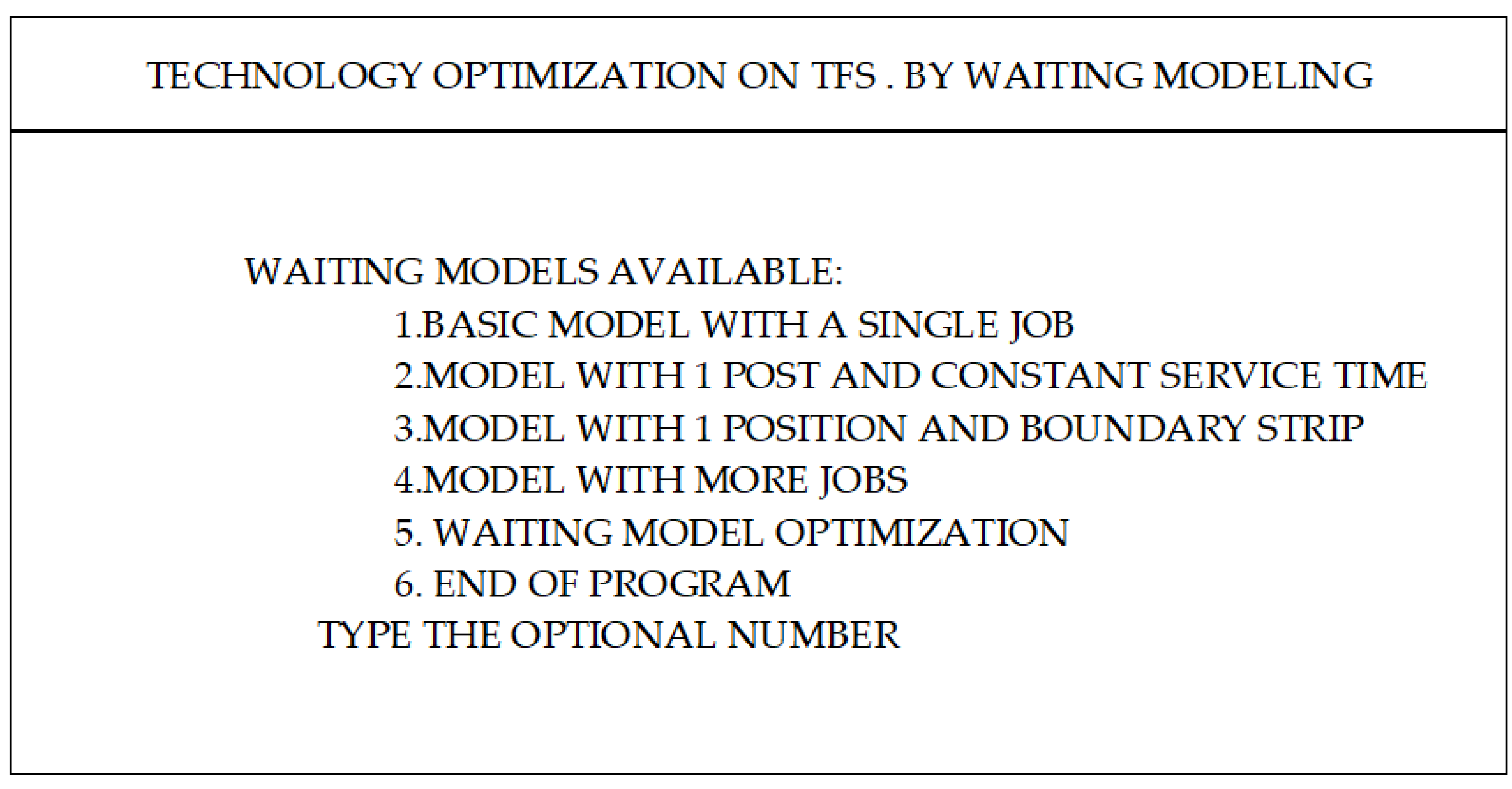
At the launch of the program, the initial choice must be made regarding the type of waiting model and whether or not only the analysis of the model is desired, as it results from the first communication screen shown in Figure 4.

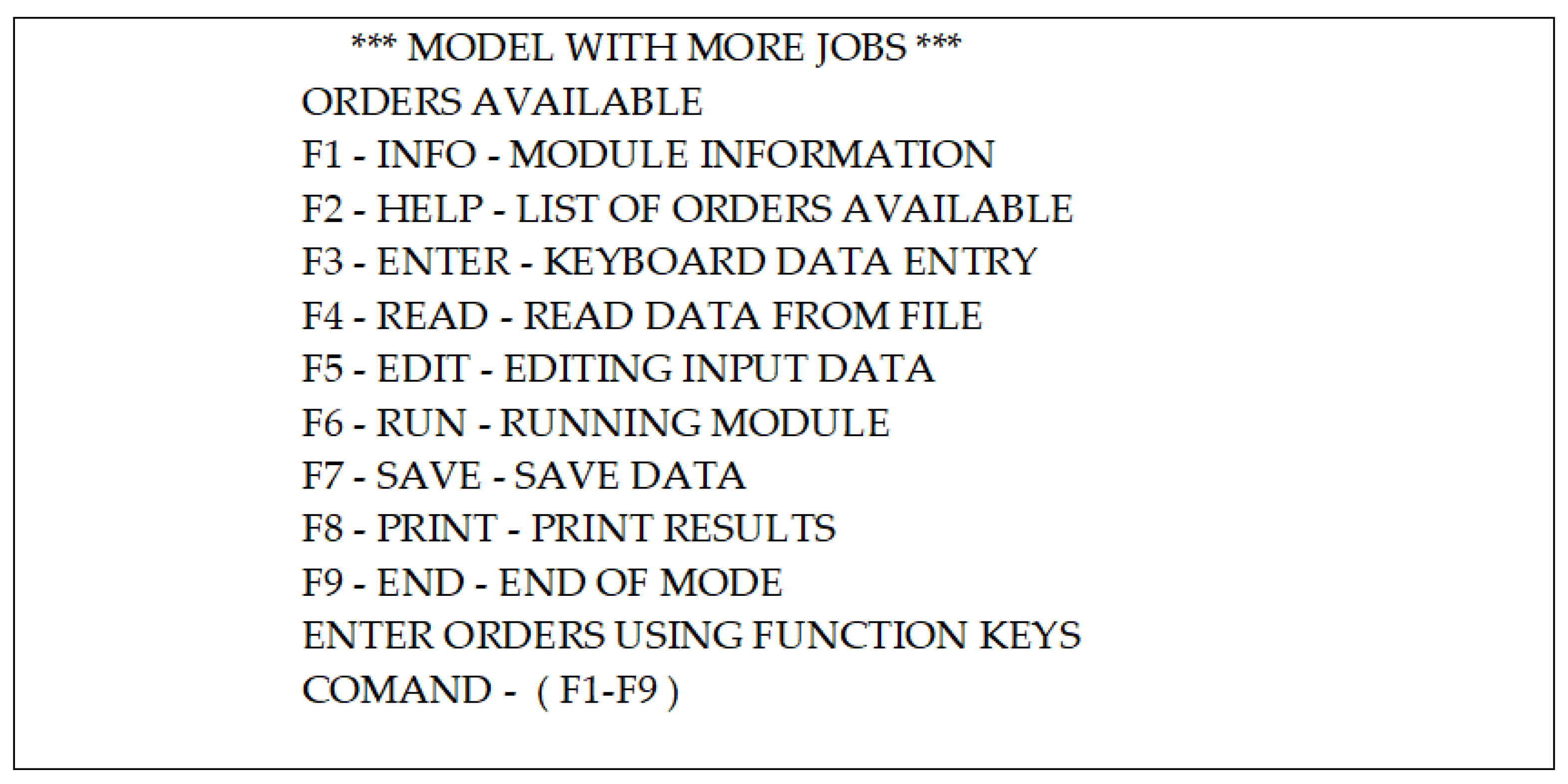
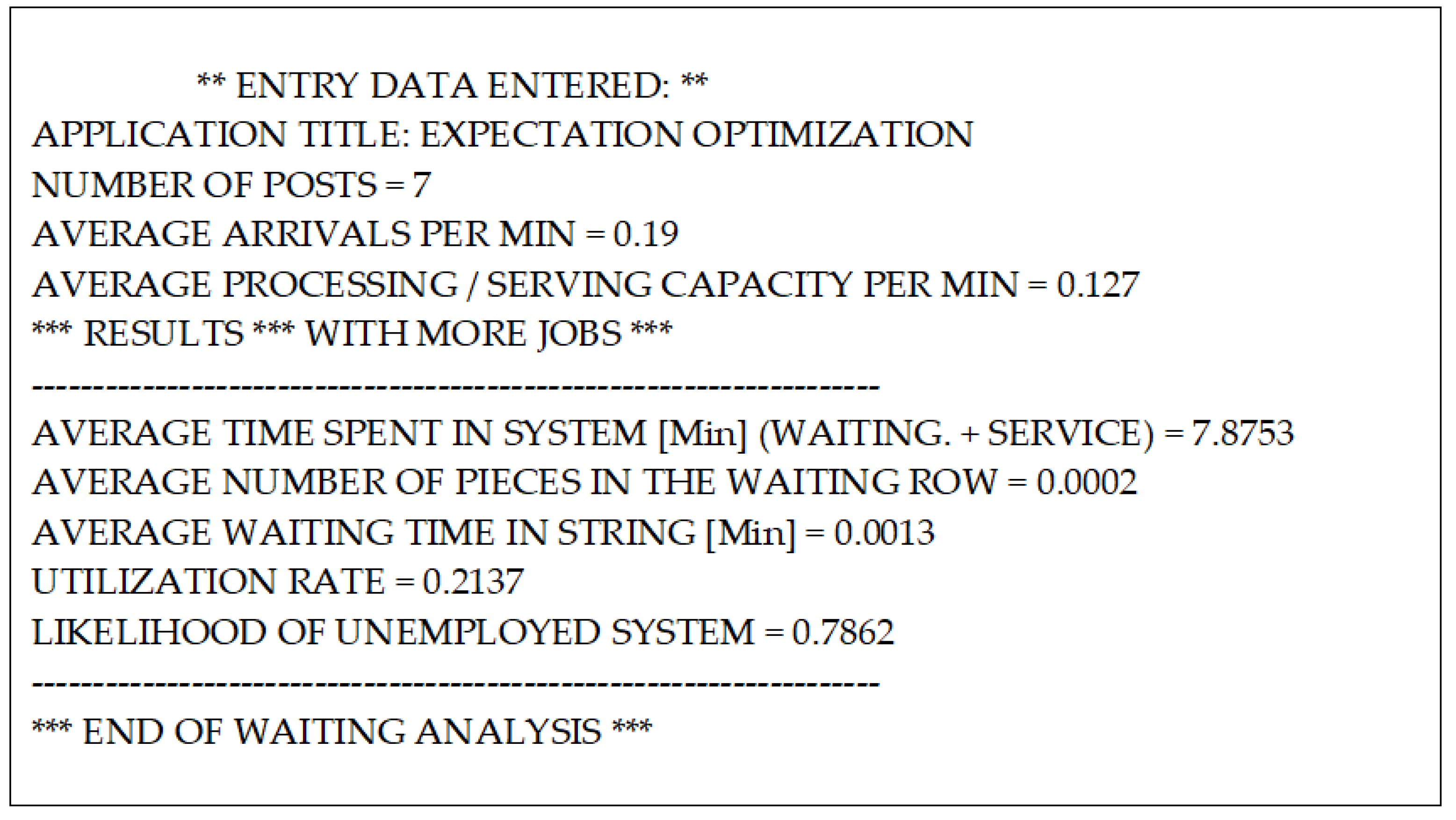
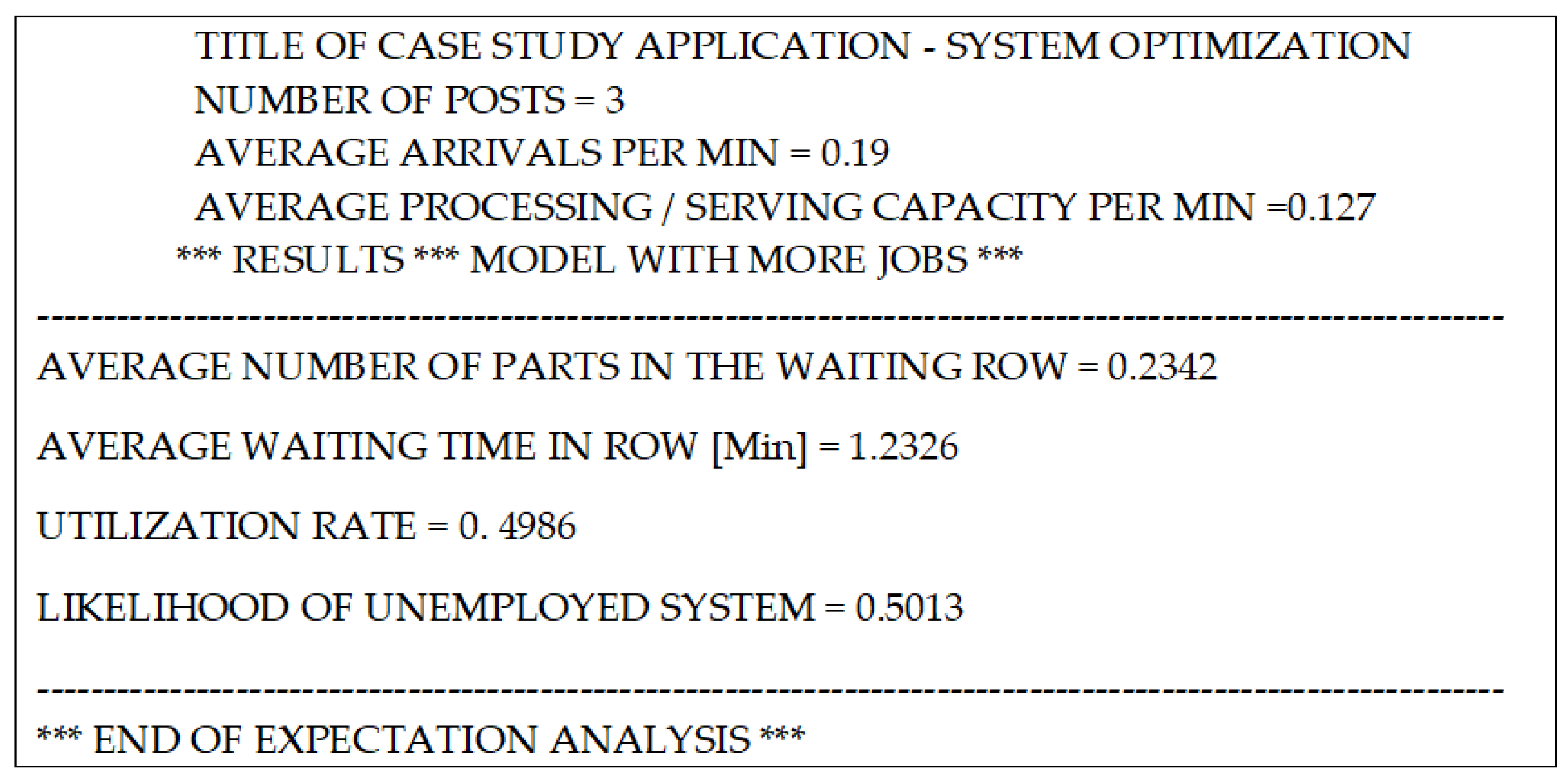
Considering that for the process of processing cylindrical teeth in the endowment of the workshop, there are, and can be used, a maximum of seven machine tools (four gear milling machines with snail milling module and three gear milling machines with a wheel knife, the rest of the machines have other destinations), we chose from block options 4 and 5. These led to the data entry stage with the options in Figure 5 and following the results in Figure 6.

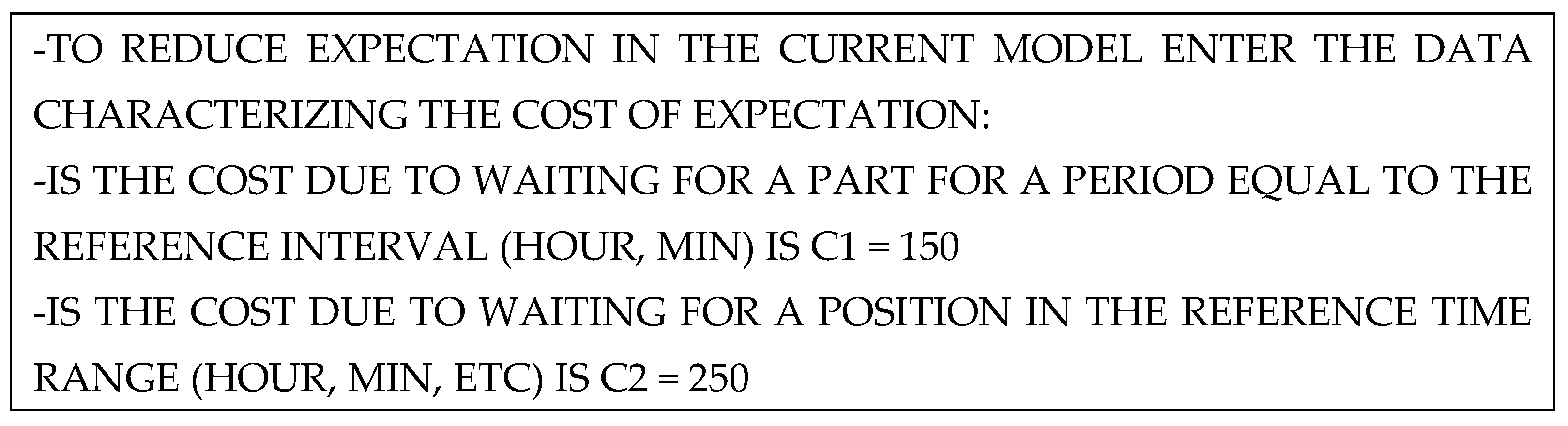
In the initial option, it was specified that in addition to the analysis of the expectations, it is desired to achieve the optimization of the waiting system in order to determine the optimal number of servers si that the expenses caused by waiting/parking machines—tools, on the one hand, and parts to be worked on, on the other hand—to be minimal, then the input data must be completed with the additional elements according to Figure 7 this resulting in the completion of the output data with the elements related to optimization, Figure 8.

In the C++ program, we simulated, during a maximum simulation period, ${\displaystyle \sum _{i=1}^m{t}_i}$ the arrivals and services. Therefore we used the variable simulation clock.

We first estimated the average number of units in the system and the average number of units in the queue as:

$$\begin{array}{l}{N}_s=\frac{{\displaystyle \sum _{i=1}^M{N}_i\ast t_i}}{{\displaystyle \sum _{i=1}^M{t}_i}}\\ N_f=\frac{{\displaystyle \sum _{i=1}^M(N_i-S)\ast t_i}}{{\displaystyle \sum _{i=1}^M{t}_i}}\end{array}$$

(12)

The other elements were computed as follows. First, we took into account that the number of units in the queue conditioned by the existence of the queue (Kleinrock, 1975) geometric distributed with parameter r. We then obtain the formula

$$p_w[S]=Nf[S]\ast \frac{1-r}{r}$$

(13)

The time spent in a queue conditioned by the existence of a queue is exponential of parameter S∗u∗(1 − r). Therefore:

$$Tf=\frac{p_w[S]}{S\ast u\ast (1-r)}$$

(14)

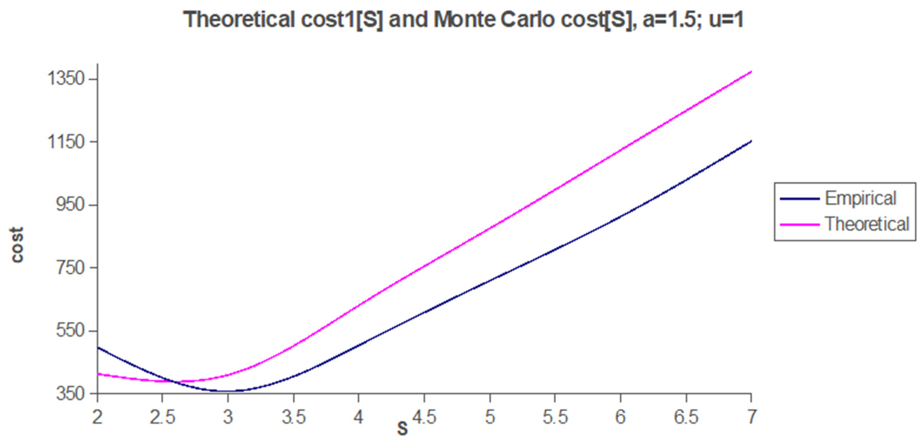
With the C++ simulation program with the same costs, C1 = 150 and C2 = 250, we first run for a maximum of seven servers in a system with one station. The first application was with a = 0.6 and u = 1. The next application was, in fact, with what we considered from the industry: a = 0.19 and u = 0.127. However, by changing the unit time, we can consider u = 1 and by proportion a = 1.5. The results are presented in Appendix B.

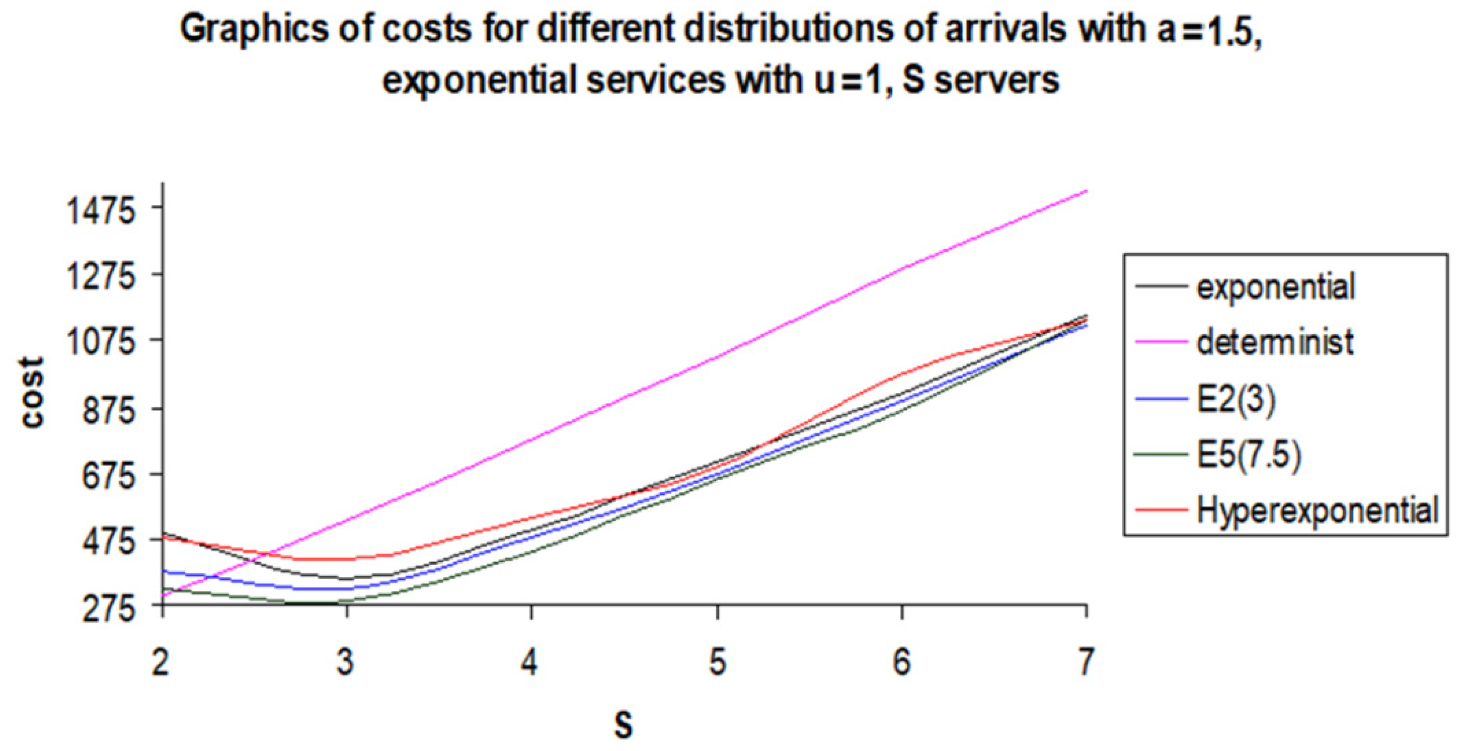
We finalized the analysis with comparative graphics of the costs with the comparative graphics of costs (Figure 9).

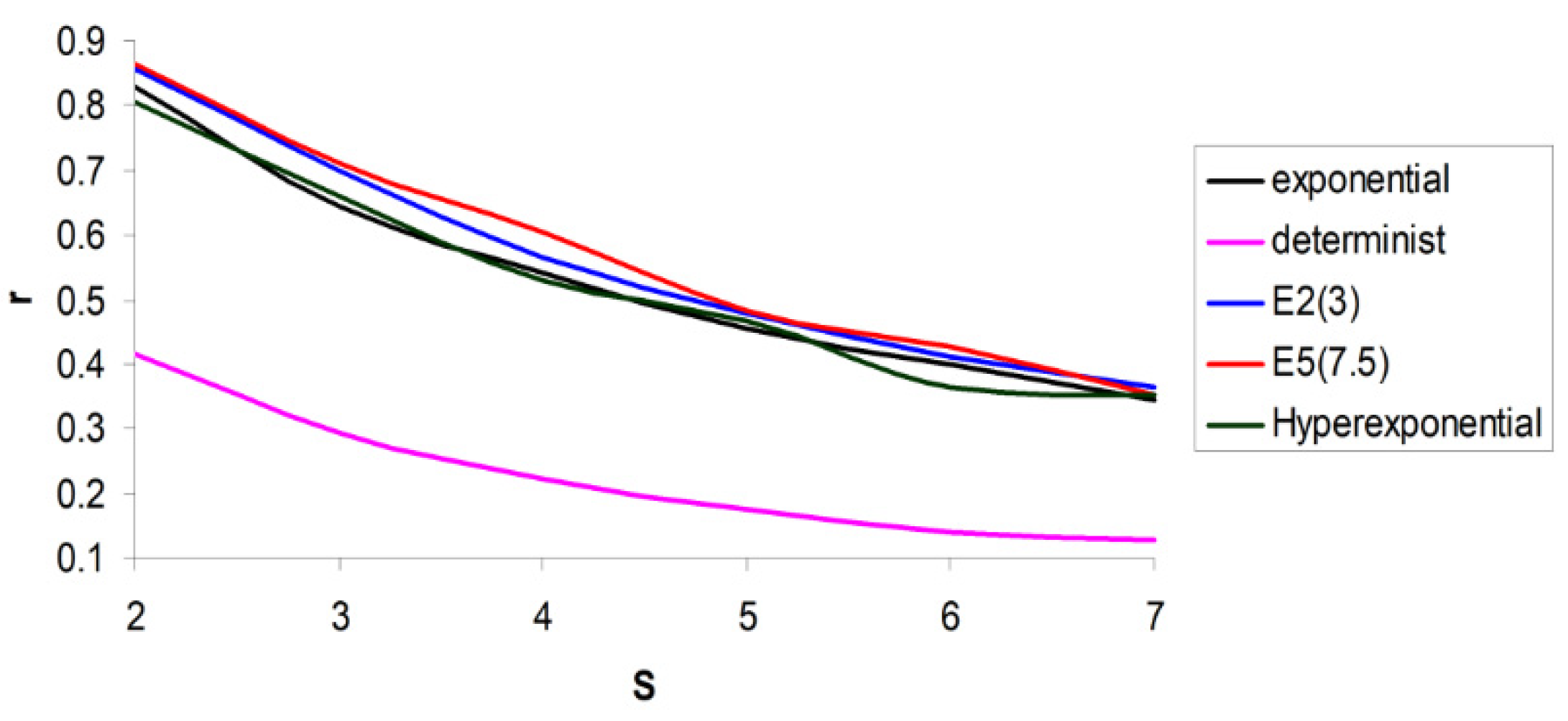
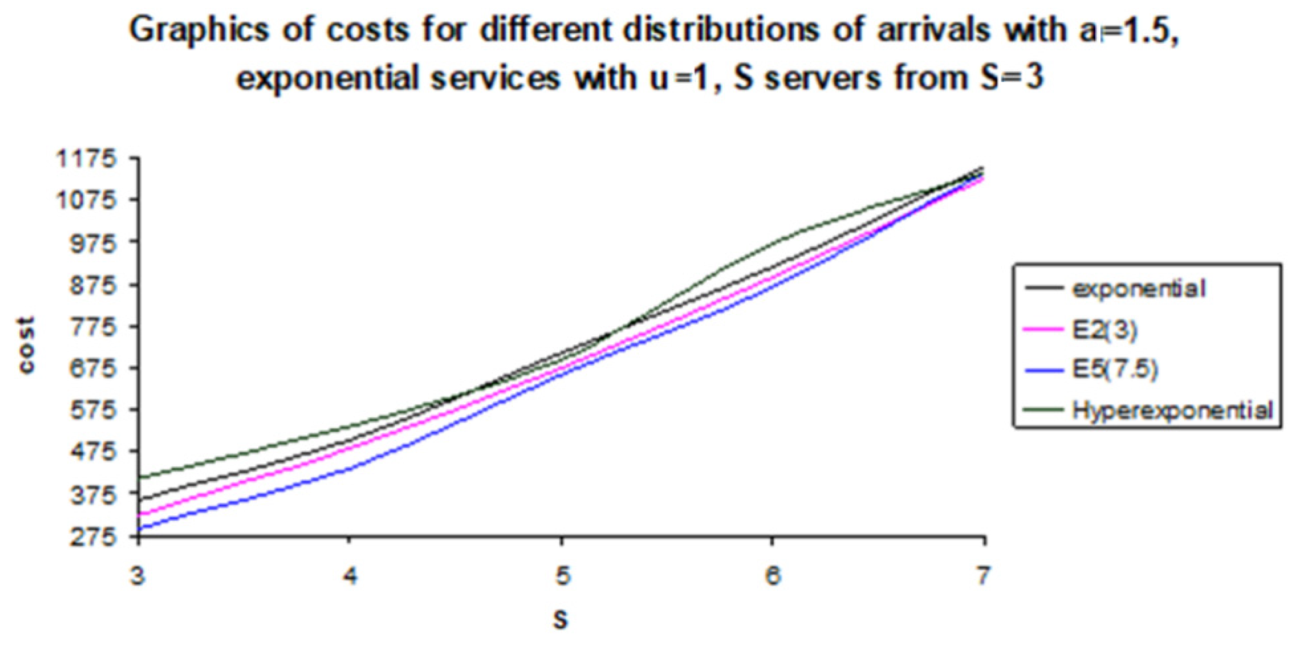
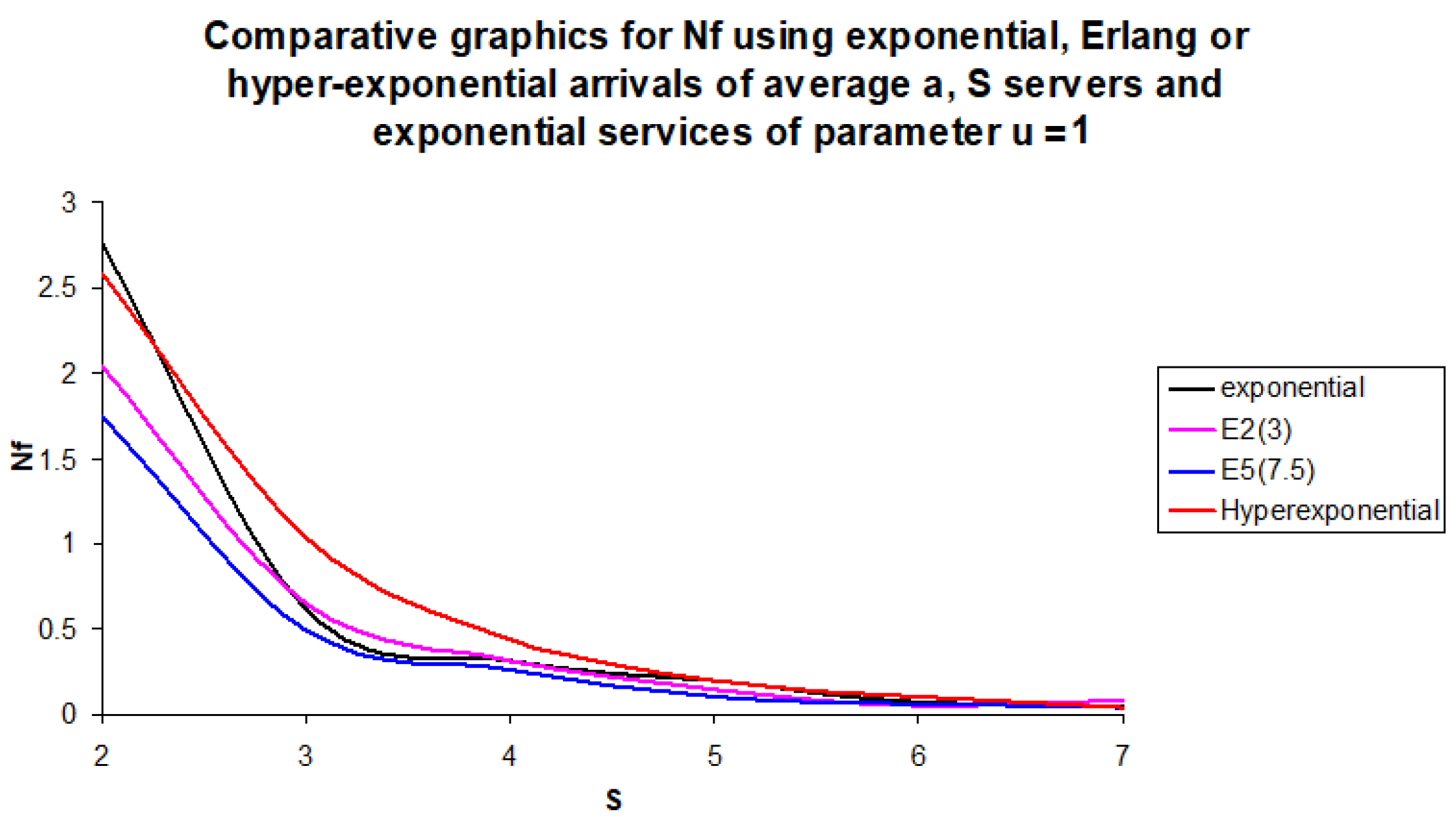
We noticed that the deterministic case is isolated. This can be explained by the fact that in this case, optimal S is 2, while in the other cases, optimal S is 3. In the following graphics (Figure 10), we represented only the non-deterministic cases.

For the costs in non-deterministic cases, the increasing order is Erlang of order 5, Erlang of order 3, and exponential. The costs in the hyper-exponential case are greater than the two Erlang cases for all S between 2 and 7. Compared with exponential, the costs are greater for S = 3, 4 or 6 and are smaller in the other cases. In the deterministic case, the cost is minimal (comparing the other distribution) only for S = 2. For S > 2, the corresponding costs are greater than the exponential case, even if we add one server in the last case. They are also greater than that of the hyper-exponential case. The same property can be noticed in the exponential case, starting from S = 4.

From S = 6, the cost is greater than all the other costs from other distributions.

5. Discussion

The following conclusions regarding the analysis and optimization of the waiting for the considered production system can be deduced both from the listing with results and from the representation of the afferent graph:

For a number of stations below the digit 2, a production overload situation occurs. This is caused by the fact that if a single serving station were used—in our case, a machine tool with a workstation—the arrival rate in the system (0.19 parts/min) would be higher than the service rate (0.127 pieces/min.), which would lead to the accumulation and continuous increase in the number of parts in the waiting string. In fact, the overload situation occurs [35] when $\frac{a}{S\ast u}>1$. Therefore the minimum S is the minimum value such the mentioned fraction is less than one. In our paper, we changed the time unit such that u = 1 (proportionally multiplying a and obtaining 1.5 instead of 0.127), and the minimum S > 1.5 is two.

Theoretically, starting from a number of two machine tools upwards (the minimum value of S such that we have no overload), we can cover the given production task, but the expenses caused by waiting/parking the parts on the one hand and the machine tools, on the other hand, have opposite influences, which leads to the existence of an optimum [36,37].

This observation is natural because the more machine tools we have with a higher processing capacity, the lower the costs of waiting for parts, the more prompt the service, and the costs of stationary machines increase due to the immobilized superior means.

The listing shows that the optimal number of machine tools that are needed to take over the given task is 3; the rest can be assigned to other production tasks. In fact, the allocation of all cars for this task would lead, as shown in the schedule, to a significant and unjustified increase in costs due to insufficient load.

Once the SOPT is known and adopted, if the analysis of the corresponding wait is desired, the data corresponding to S = 3 can be called directly from the program, as is shown in Figure 11.

These new values lead to a better loading of the technological system compared to the situation of the preliminary study when, without adopting a correctly studied technological decision, we allocated the entire production capacity to the given task.

It should be noted that in technological systems working with variable production loads and in the assumptions initially presented, much lower loads are usual than in the case of those working in large series and mass production, which are not the subject of this study.

The minimum number of machines, which would ensure the maximum load of the system, does not necessarily lead to the optimal solution in terms of waiting costs, as is shown in the example given.

By changing the values of costs C1 and C2 regarding the waiting of parts and machine tools in the reference time unit and taking into account the general expression of the waiting cost function, we noticed that we could be in one of the following situations (Figure 12a–c).

The case in Figure 12a is, in fact, the most general case, which also corresponds to the analyzed example, and it is encountered when the influences of the waiting costs C₁ and C₂ are comparable, and the number of servers is large enough for both to be able to manifest. There is a first decreasing portion—corresponding to the small number of servers—where the costs of waiting for parts are predominant, an optimal level followed by an increasing slope, corresponding to the area with a large number of servers, where the costs of waiting are predominant.

The second case (Figure 12b) occurs when we have a small number of servers. It actually corresponds to the first part of the general chart and has the disadvantage that we cannot know if the minimum is reached for the maximum number of servers we have or if it is only to be reached.

This situation is also encountered when the high share is the cost of waiting for the C₁ part; for example, for an urgent production task whose delay in completion can lead to significant penalties. In these cases, either an additional capacity is sought (if this is possible) by increasing S and identifying S_opt, as recommended in the calculation of the calculation program, or directly choose the value S_opt = S_max as a value that ensures the minimum losses under the given conditions.

Finally, the third case (Figure 12) corresponds to the situation when the maximum share of losses comes from the parking of the machine tools in a system with a low load, in which the waiting phenomenon of the parts is less important.

This situation is most common in complex, high-capacity industrial systems, where large initial investments and potential loans lead to significant losses caused by downtime. Obviously, in this situation, the optimal decision is made, as it results from the listing in Figure 11 at the values S_opt = S_min, seeking to release as much of the production capacity as possible in order to focus on other tasks.

We also made a comparison of the distribution of the inter-arrival times. The optimum S was 3, except in the case of deterministic arrivals, which is minimum plus one. In the deterministic case, the minimum S such that a/(S∗u) < 1 is also optimal.

We also found an increasing order of the cost for the same S for exponential distribution and Erlang distributions: E₅, E₂ and exponential. The same order is for Nf, except S = 6 between E₅ and E₂ and S = 3 or S = 7 between E₂ and exp, as we can see in the following picture (Figure 13).

The rule of having greater cost (in the case of the above picture, the waiting cost) for hyper-exponential than for exponential has the same three exceptions as in the case of total costs: S = 2, S = 5 and S = 7.

In the deterministic case, N_f is very small comparing the non-deterministic case: for S = 2, it is smaller than all other cases for S = 6. The reason for not having the smallest cost in the deterministic case is that r is also the smallest, as we can see in the picture (Figure 14).

We noticed the same isolation in minimum for r of the determinist case as the total maximum cost in Figure 14.

The increasing order of r is determinist, hyper-exponential and exponential for E₂, E₅ and even S (2, 4 or 6), with a switch between exponential and hyper-exponential for odd S.

6. Conclusions

Generally, we noticed smaller costs and N_f for Erlang cases compared with exponential and hyper-exponential cases (with the mentioned exceptions) and higher values of r. Between exponential and hyper-exponential cases, the smallest cost and the smallest Nf are the hyper-exponential for S = 2, S = 5 or S = 7. When comparing the values of r for these distributions, they are higher in the hyper-exponential case for S odd. Therefore, none of these distributions are better. We also notice that the highest costs in the deterministic case are due to the lowest values of r (Figure 14).

With our C++ program for Jackson queueing networks, we read the number of nodes from the keyboard. We read the transition matrix (the probabilities that after finishing service in node i go to node j/living network) and the average number of arrivals/time unit for each node from a text file. With these data, we computed the matrix and the right sides for the involved linear system, which we solved using the mentioned Gauss–Seidel method.

Based on these observations and considerations, it can be concluded that the proposed method, algorithm and program can contribute to the optimization in terms of technological times of the operation of technological manufacturing systems, taking into account from the stage of manufacturing preparation the global influences that they have the waiting phenomena in the system on the efficiency of the technological process. However, as has been mentioned before, after applying the optimization strategy presented in the paper, a correctly and optimally sized enterprise was obtained. This aspect is likely to help (even if indirectly) the ZDM concept of the fact that a correctly and optimally sized enterprise can also lead to optimal results in manufacturing and through the prism of the ZDM concept. It will not have overloaded STF or used artificially/inappropriately in certain technologies but will have the optimal endowment (in terms of type and capacity), which also favors the ZDF standard, implicitly ensuring increased sustainability both from a technological and logistical point of view.

In addition, through the method presented and exemplified in the case study, a quick and easy-to-use working tool was created, through which the waiting phenomena in industrial systems can be studied and coordinated in real time, creating the conditions elimination of arbitrariness in the process of adopting the technological decision in the analyzed field.

Classical software such as Management Scientist has implemented only the classical S servers queueing system with Poisson arrivals (and, of course, exponential services in the literature). The optim “economic analysis” performs the computation of the total cost as in this paper. We proved the observed bimodal monotony (first decreasing and next increasing) of this cost in terms of S. In this paper, we found a condition for S in which, from that point, the cost increases. Therefore, we obtained an upper limit for optimal S, and the real optimal S is obtained by comparison of all costs until the upper limit. Initially, the total cost depends on three elements: the expected number of units in the queue, activity rate and the number of servers, S. However, all the other two depend on S; hence the optimization problem is to minimize one variable function.

In large series and mass manufacturing, the design of the enterprise is based on the specifics of this type of production, the repeatability/constant in a time of the operations and processing provided in the technology of the parts from the manufacturing series. Thus, there are precise rules according to which the sizing of the enterprise can be performed exactly and adequately to the respective flow/production.

However, things become complicated when the manufacture is differentiated, and it varies from month to month, often from one week to the next or even from one day to the next. It was found that in order to have optimal results in production, the sizing/endowment of enterprises subject to variable tasks must be performed by taking into account the specifics of input flows of parts (aspects analyzed in our paper) and not by other random criteria.

References

1. Ferney, M. Techniques d’ordonnancement; Ecole Nationale d’ Ingenieurs de Belfort: Belfort, France, 1996. [Google Scholar]
2. Mihoc, G.; Ciucu, G.; Muja, A. Mathematical Models of the Waiting Theory; Publishing House of the Romanian Academy: Bucharest, Romania, 1983. [Google Scholar]
3. Johnston, A.; Lang, E.; Innes, G. The waiting game: Managing flow by applying queueing theory in Canadian emergency departments. Can. J. Emerg. Med. 2022, 24, 355–356. [Google Scholar] [CrossRef] [PubMed]
4. Glynn, P.W. Queueing theory: Past, present, and future. Queueing Syst. 2022, 100, 169–171. [Google Scholar] [CrossRef]
5. Walton, N. Queueing: A perennial theory. Queueing Syst. 2022, 100, 557–559. [Google Scholar] [CrossRef]
6. Jain, S.; Jain, R. Application of Queuing Theory in Quality Management Practices in Medical Sector. J. Algebraic Stat. 2022, 13, 487–496. [Google Scholar]
7. Goncalves, P. Back to basics: Fundamental principles of system dynamics and queueing theory. Syst. Dyn. Rev. 2022, 38, 81–92. [Google Scholar] [CrossRef]
8. Ciuiu, D. Solving Linear Systems of Equations and Differential Equations with Partial Derivatives by the Monte Carlo Method using Service Systems; Analele Universităţii Bucureşti: Bucharest, Romania, 2004; pp. 93–104. [Google Scholar]
9. Liu, F.J.; Ma, Z.Y.; Si, Q.N.; Yan, M. Performance analysis of peer-to-peer networks based on two-phase service queuing theory. Int. J. Commun. Netw. Distrib. Syst. 2021, 27, 349–365. [Google Scholar] [CrossRef]
10. Salawu, G.; Bright, G.; Onunka, C. Performance Optimisation on Waiting Time Using Queueing Theory in An Advanced Manufacturing Environment. S. Afr. J. Ind. Eng. 2020, 31, 9–18. [Google Scholar] [CrossRef]
11. Dorda, M.; Teichmann, D.; Graf, V. Optimisation of Service Capacity based on Queueing Theory. MM Sci. J. 2019, 2019, 2975–2981. [Google Scholar] [CrossRef]
12. Chen, C.; Tiong, L.K. Using queuing theory and simulated annealing to design the facility layout in an AGV-based modular manufacturing system. Int. J. Prod. Res. 2019, 57, 5538–5555. [Google Scholar] [CrossRef]
13. Forghani, K.Z.; Ghomi, S.M.T.F. A queuing theory-based approach to designing cellular manufacturing systems. Sci. Iran. 2019, 26, 1865–1880. [Google Scholar]
14. Lasrado, V.; Nazzal, D. Design of A Manufacturing Facility Layout with A Closed Loop Conveyor with Shortcuts Using Queueing Theory and Genetic Algorithms. In Proceedings of the Winter Simulation Conference (WSC)/Conference on Modeling and Analysis for Semiconductor Manufacturing (MASM), Phoenix, AZ, USA, 11–14 December 2011; pp. 1959–1970. [Google Scholar]
15. Schelasin, R. Using Static Capacity Modeling and Queuing Theory Equations to Predict Factory Cycle Time Performance in Semiconductor Manufacturing. In Proceedings of the Winter Simulation Conference (WSC)/Conference on Modeling and Analysis for Semiconductor Manufacturing (MASM), Phoenix, AZ, USA, 11–14 December 2011; pp. 2040–2049. [Google Scholar]
16. Shanthikumar, J.G.; Ding, S.W.; Zhang, M.T. Queueing theory for semiconductor manufacturing systems: A survey and open problems. In Proceedings of the IEEE Transactions on Automation Science and Engineering, Scottsdale, AZ, USA, 22–25 September 2007; Volume 4, pp. 513–522. [Google Scholar] [CrossRef]
17. Govil, M.K.; Fu, M.C. Queueing theory in manufacturing: A survey. J. Manuf. Syst. 1999, 18, 214–240. [Google Scholar] [CrossRef]
18. Raviv, A. Optimal staffing in semiconductor manufacturing: A queuing theory approach. Solid State Technol. 1998, 41, 77–87. [Google Scholar]
19. Papadopoulos, H.T.; Heavey, C. Queueing theory in manufacturing systems analysis and design: A classification of models for production and transfer lines. Eur. J. Oper. Res. 1996, 92, 1–27. [Google Scholar] [CrossRef]
20. Atkinson, B.; Papadopoulos, H.T.; Heavey, C.; Browne, J. Queuing Theory in Manufacturing Systems-Analysis and Design. J. Oper. Res. Soc. 1995, 46, 137–138. [Google Scholar]
21. Hitomi, K.; Nakajima, M.; Osaka, Y. Analysis of Flow-Type Manufacturing Systems Using Cyclic Queuing Theory. J. Eng. Ind. 1978, 100, 468–474. [Google Scholar] [CrossRef]
22. Stolyar, A. Large-scale heterogeneous service systems with general packing constraints. Adv. Appl. Probab. 2017, 49, 61–83. [Google Scholar] [CrossRef] [Green Version]
23. Powell, D.; Magnanini, M.C.; Colledani, M.; Myklebust, O. Advancing zero defect manufacturing: A state-of-the-art perspective and future research directions. Comput. Ind. 2022, 136, 103596. [Google Scholar] [CrossRef]
24. Psarommatis, F.; May, G.; Dreyfus, P.A.; Kiritsis, D. Zero defect manufacturing: State-of-the-art review, shortcomings and future directions in research. Int. J. Prod. Res. 2020, 58, 1–17. [Google Scholar] [CrossRef]
25. Connor, S.; Kendall, W. Perfect simulation of M/G/c queues. Adv. Appl. Probab. 2015, 47, 1039–1063. [Google Scholar] [CrossRef] [Green Version]
26. Mihoc, G.; Nădejde, I. Introduction in the Waiting Theory; Tehnical Publishing House: Bucharest, Romania, 1980. [Google Scholar]
27. Garzia, M.; Garzia, R.; Kiemele, M.; Lockhart, C. Network Modeling, Simulation and Analysys; Marcel Deker: New York, NY, USA; Basel, Switzerland, 1990. [Google Scholar]
28. Iosifescu, M. Lanturi Markov Finite si Aplicatii; Tehnica: Bucuresti, Romania, 1977. [Google Scholar]
29. Goswami, C.; Selvaraju, N. Phase-Type Arrivals and Impatient Customers in Multiserver Queue with Multiple Working Vacations. Adv. Oper. Res. 2016, 2016, 4024950. [Google Scholar] [CrossRef]
30. Koops, D.T.; Saxena, M.; Boxma, O.J.; Mandjes, M. Infinite Server Queues with Hawkes input. J. Appl. Probab. 2018, 55, 920–949. [Google Scholar] [CrossRef] [Green Version]
31. Carabulea, A.; Rușitoru, A. Optimizarea Conducerii Sistemelor Industriale; Editura Didactică Şi Pedagogică: București, Romania, 1986. [Google Scholar]
32. Ciuiu, D. A Method to Solve Some Nonlinear Equations by the Monte Carlo Method Using Queueing Systems. Ann. Univ. Bucur. 2006, 1, 21–30. [Google Scholar]
33. Rece, L.; Florescu, V.; Modrea, A.; Jeflea, V.; Harnicarova, M.; Valicek, I.; Borzan, M. Optimization of the 2 1/2 D Processing Method of Complex Parts, through a Predictive Algorithm for Controlling the Geometric Shape Deviations Resulting from Processing. Mathematics 2020, 8, 59. [Google Scholar] [CrossRef] [Green Version]
34. Kleinrock, L. Queueing Systems; John Wiley and Sons: Hoboken, NJ, USA, 1975. [Google Scholar]
35. Vaduva, I. Modele de Simulare; Universitatii Bucuresti: Bucuresti, Romania, 2004. [Google Scholar]
36. Lee, A.M. Applied Queueing Theory; The Macmillan Pr. Ltd.: London, UK, 1996. [Google Scholar]
37. Ciuiu, D. The Jackson Queueing Network Built Using Poisson Measures. Application To A Bank Model. Folia Oeconomica Stetin. 2013, 13, 7–22. [Google Scholar] [CrossRef] [Green Version]
Figure 1. Value as optimal based on the existence of contradictory tendencies.
Mathematics 10 02520 g001
Figure 2. The flow-based processing.
Mathematics 10 02520 g002
Figure 3. (a) Real factory case, which is small series manufactured at a real factory. (b) Reference machines of each category from the analyzed production department.
Mathematics 10 02520 g003aMathematics 10 02520 g003b
Figure 4. The first communication screen.
Mathematics 10 02520 g004
Figure 5. Data entry stage with the options.
Mathematics 10 02520 g005
Figure 6. The results for the PP7 queueing system.
Mathematics 10 02520 g006
Figure 7. The input data completed with the additional elements.
Mathematics 10 02520 g007
Figure 8. The output data with the elements related to optimization.
Mathematics 10 02520 g008
Figure 9. Graphics of costs for different distributions of arrivals, in terms of S.
Mathematics 10 02520 g009
Figure 10. Graphics of costs for different distributions of arrivals.
Mathematics 10 02520 g010
Figure 11. The optimal results for SOPT.
Mathematics 10 02520 g011
Figure 12. (a) The number of servers is large. (b) The number of servers is small. (c) The system has low load. (ac) The values of costs C1 and C2 regarding the waiting of parts and machine tools in the reference time unit.
Mathematics 10 02520 g012
Figure 13. Comparative graphics for Nf.
Mathematics 10 02520 g013
Figure 14. Comparative graphics of r for some distributions of inter-arrival times with a = 1.5; u = 1.
Mathematics 10 02520 g014