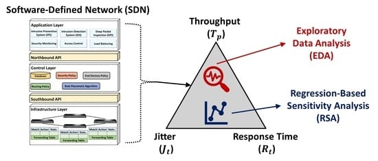
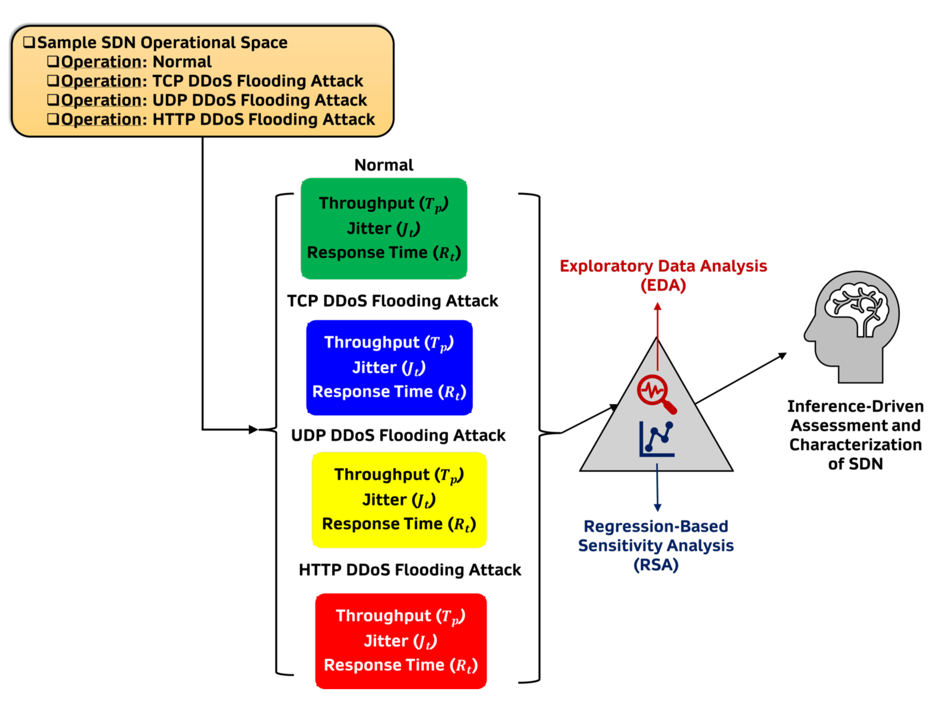
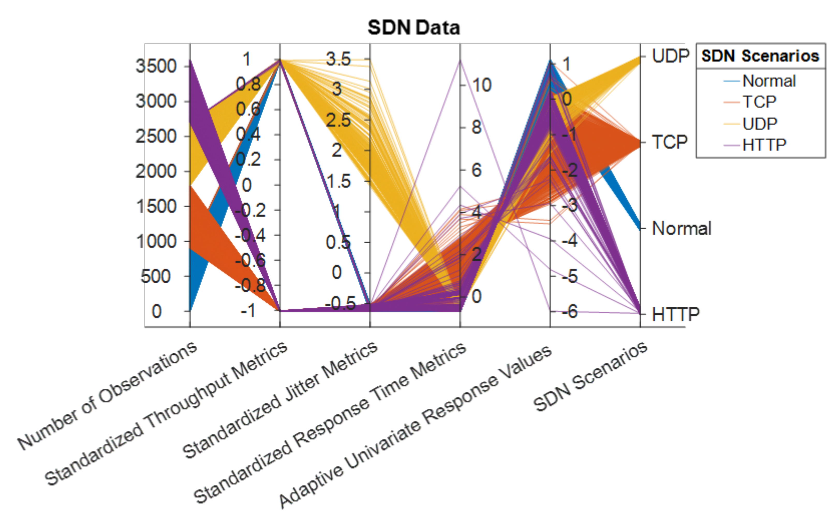
In this section, the SDN performance metrics generated based on the SDN configuration discussed, and the experiments conducted in
Section 3 are visualized and critically investigated via univariate and multivariate, graphical, and non-graphical EDA methods. EDA methods such as descriptive statistics and histograms are at the core of data science, and they have been widely used for the analysis, visualization and interpretation of data [
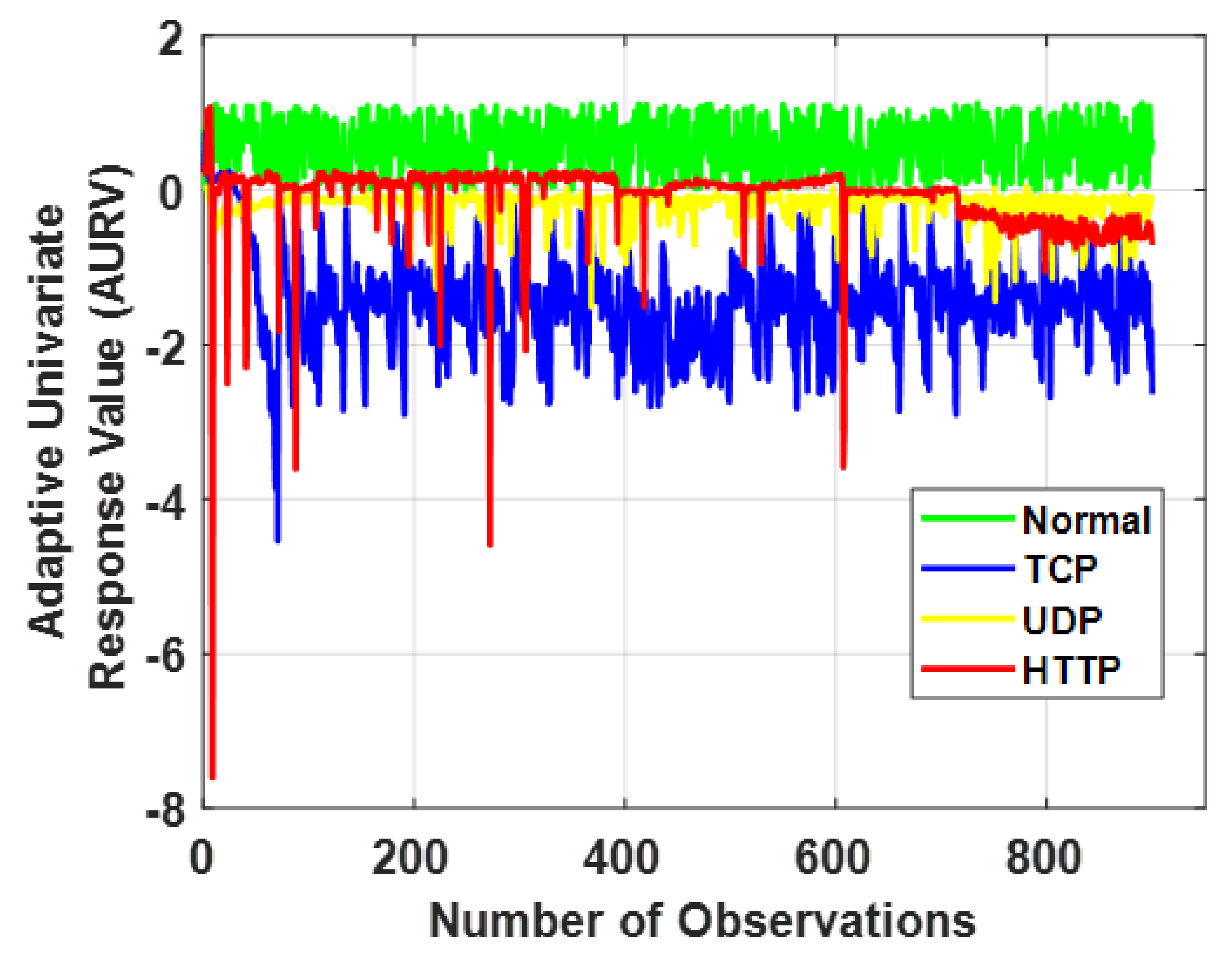
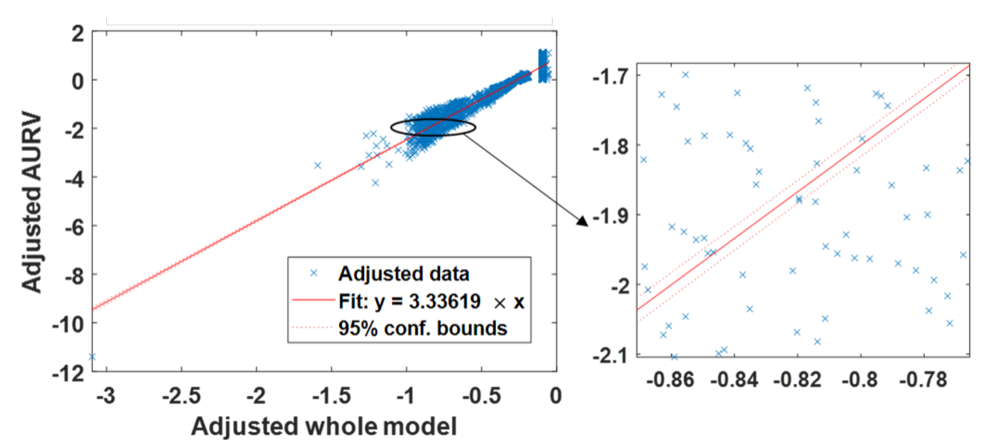
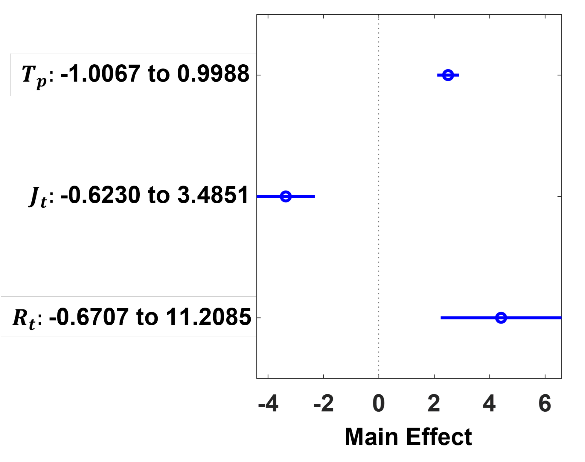
26]. For a more robust analysis of the SDN performance metrics, RSA is conducted by fitting a linear regression model to understand and statistically account for the pairwise interactions between the jitter (
), response time (
) and throughput (
) metrics of the emulated SDN when it is operating without attack (“Normal” state) and when it is subjected to HTTP DDoS flooding attacking (“HTTP” state), TCP DDoS flooding attack (“TCP” state) and UDP DDoS flooding attacking (“UDP” state). All experiments analyzed and discussed in this section have been carried out on a workstation with Intel 6-core i7-8700 3.20 GHz CPU and 32.0 GB RAM, except where stated otherwise. The elapsed times reported are elapsed real times from a wall clock.
5.2. Distributions of the SDN Parameters
To visualize the distributions of the SDN parameters under consideration for the SDN scenarios described in
Section 3, histograms with distribution fits based on probability density function (PDF) are used. The visualizations are shown in
Figure 4,
Figure 5 and
Figure 6. The PDFs for the normal distributions in
Figure 4,
Figure 5 and
Figure 6 with mean (
), standard deviation (
), and variance (
) are derived as follows:
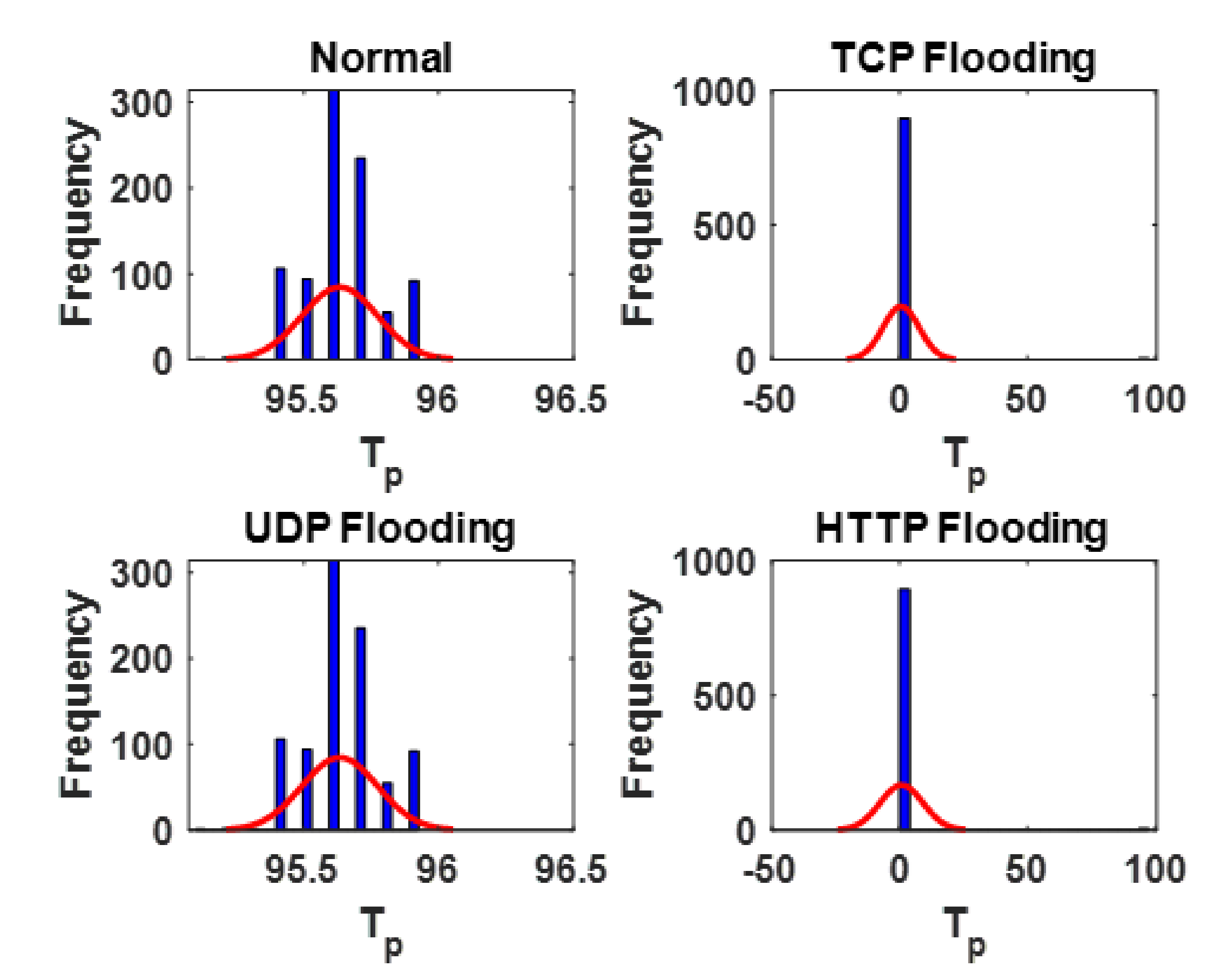
From
Figure 4, the following inferences can be made for
: (1)
is affected or altered when the SDN is subjected to a DDoS flooding attack. (2) The distribution of
did not change or vary noticeably when the SDN is subjected to UDP flooding attack. (3) The distribution of
changed or varied noticeably when the SDN is subjected to TCP flooding and HTTP flooding attacks with most of the metrics distributed around 0, as opposed to the range of around 95 to around 96, when the SDN is operating normally or subjected to UDP flooding attack. From a practical viewpoint, in
Figure 4,
can be said to be more susceptible to TCP and HTTP flooding attacks due to the way in which TCP and HTTP flooding attacks work—bombardment of the target server with multiple connection requests to consume the server’s network resources and inundation of the target server with multiple browser-based internet requests that will eventually cause denial-of-service to additional legitimate requests, respectively [
27,
28]. In a sense,
is typically affected in these scenarios. However, a scenario in which the targeted server utilizes resources to check and then responds to each received UDP packet, including spoofed UDP packets, as in the case of the UDP flooding attack, may not necessarily affect
.
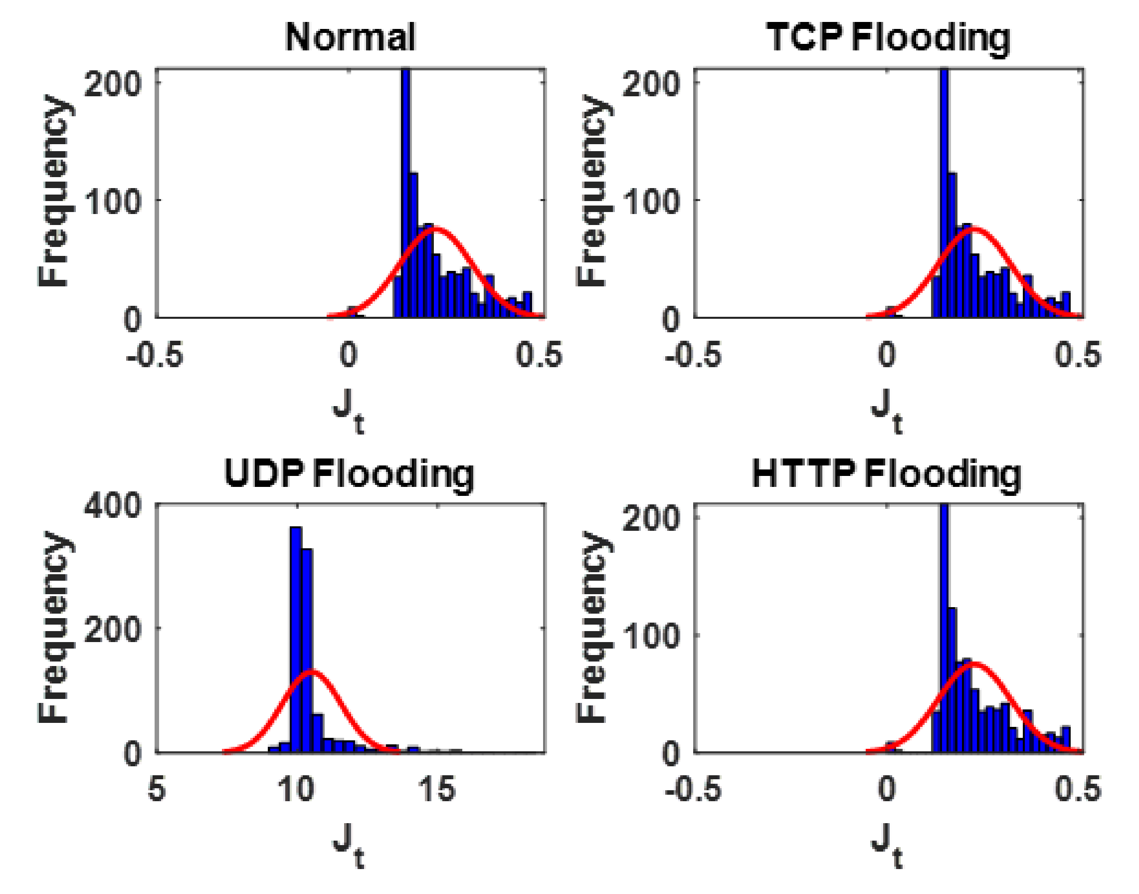
From
Figure 5, the following inferences can be made for
: (1)
is affected or altered when the SDN is subjected to a DDoS flooding attack. (2) The distribution of
did not change or vary noticeably when the SDN is subjected to TCP flooding and HTTP flooding attacks. (3) The distribution of
changed or varied noticeably when the SDN is subjected to UDP flooding attack with most of the metrics distributed over the range of around to around 15, as opposed to the range of around 0 to around 0.5, when the SDN is operating normally or subjected to TCP flooding attack or subjected to HTTP flooding attack. Jitter is all about timing and the sequence of the arriving packets. If packets arrive in bursts interspersed with gaps, or if they arrive out of sequence, then jitter values will be high. From a practical viewpoint, in
Figure 5,
can be said to be more susceptible to UDP DDoS flooding attack due to the way in which UDP DDoS flooding attacks work—a handshake is not required, and the targeted server is flooded with UDP traffic without first getting the server’s permission to initiate communication [
29]. In a sense,
and
are typically not affected in this scenario. However, the impact of the UDP DDoS flooding attack can be more severe when running voice over IP (VoIP) applications [
30].
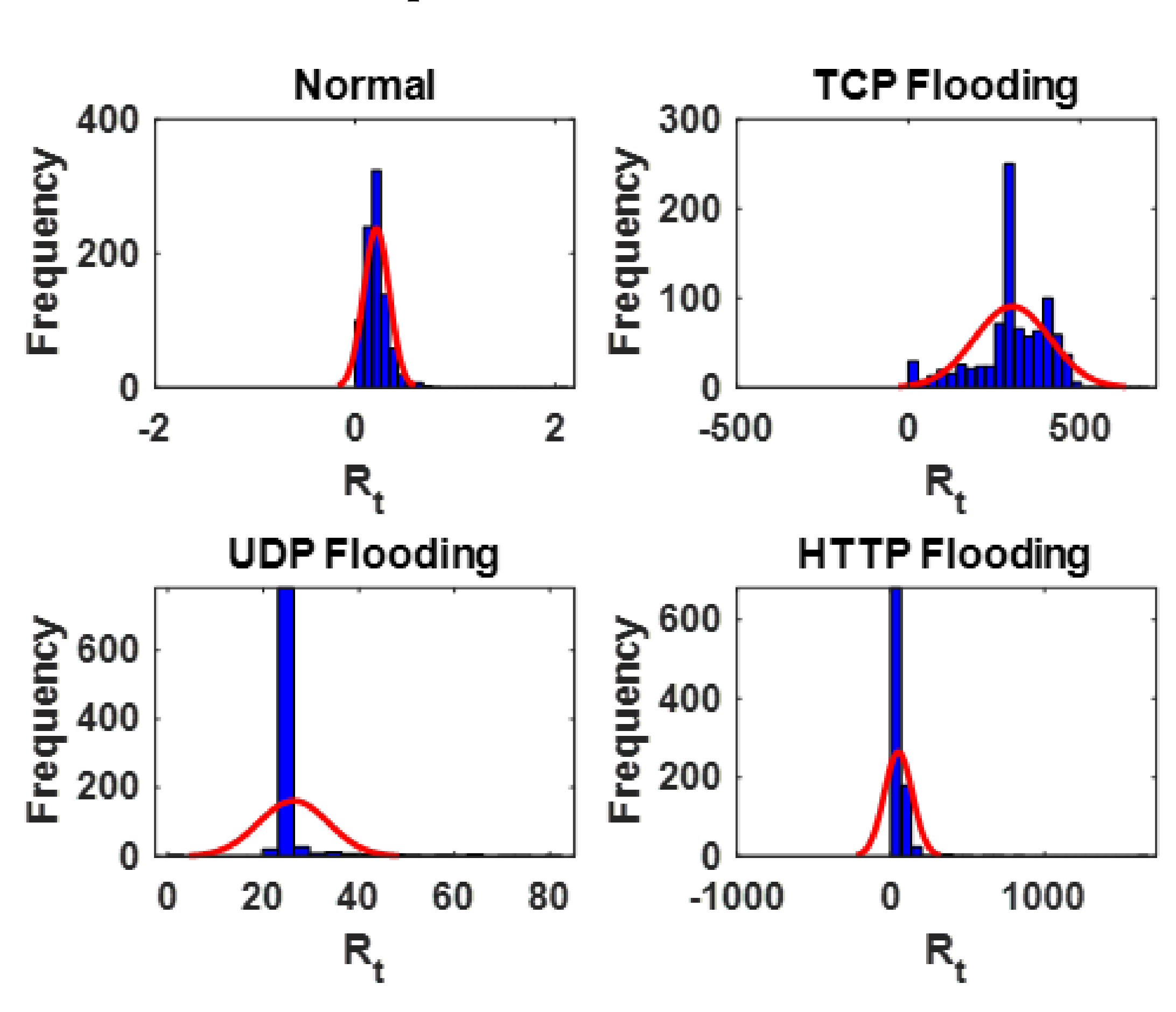
From
Figure 6, the following inferences can be made for
: (1)
is affected or altered when the SDN is subjected to a DDoS flooding attack. (2) The distribution of
changed or varied noticeably when the SDN is subjected to TCP flooding, UDP and HTTP flooding attacks. (3) Most of the metrics are distributed over a range of around 0 to around 500 for TCP flooding attack, a range of around 10 to around 50 for UDP flooding attack, and a range of around 0 to around 200 for HTTP flooding attack, in sharp contrast to a range of around 0 to around 0.5, when the SDN is operating normally. From a practical viewpoint, in
Figure 6,
can be said to be susceptible to all the investigated DDoS flooding attacks (TCP, UDP and HTTP) due to the nature of these attacks (already discussed above) [
27,
28,
29]. As a result,
is a critical network monitoring metric, and it can be drastically affected by DDoS flooding attacks, especially in applications that require waiting for an acknowledgement before sending any more packets. In such situations, the unified communication systems of SDNs are often hampered.
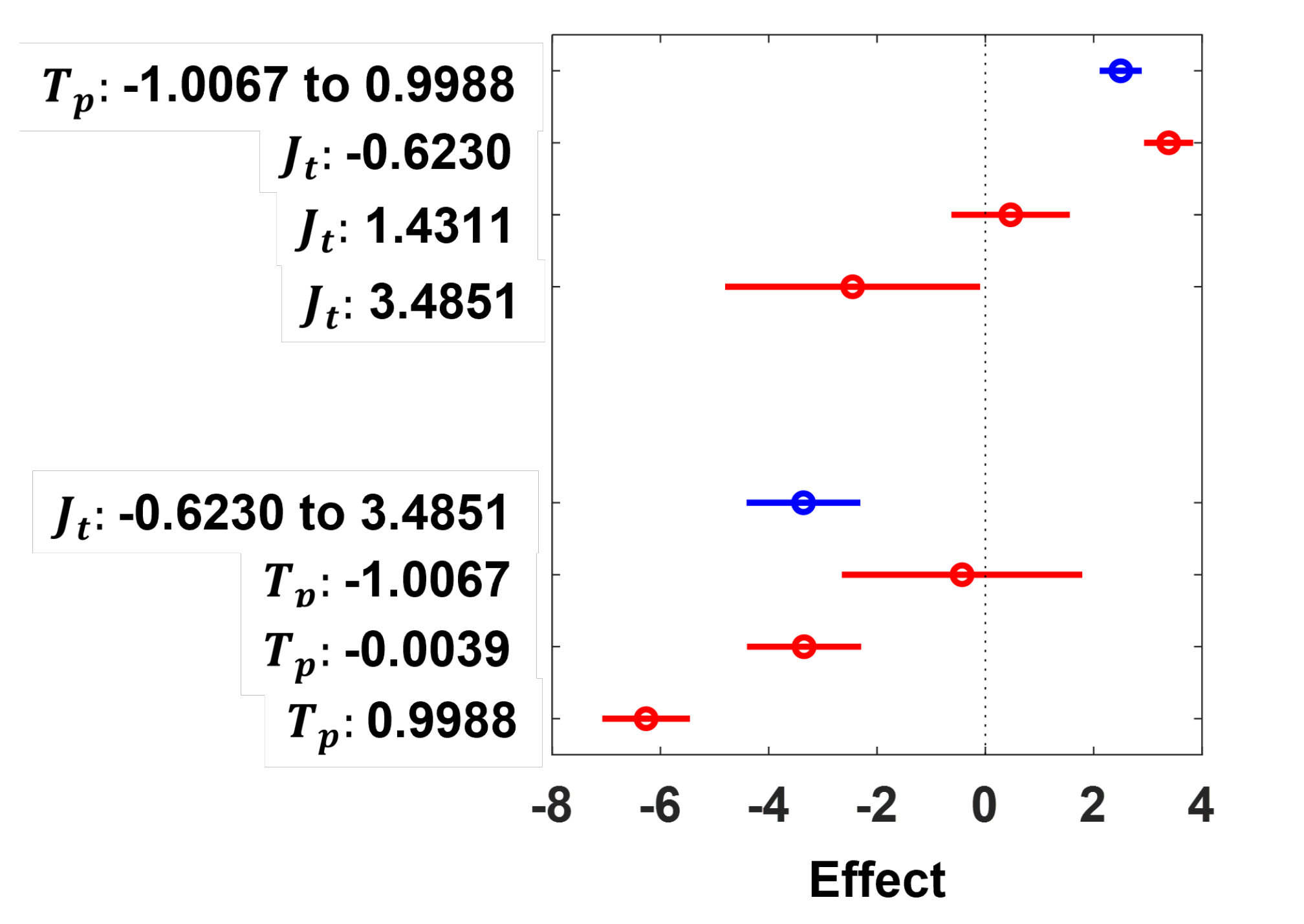
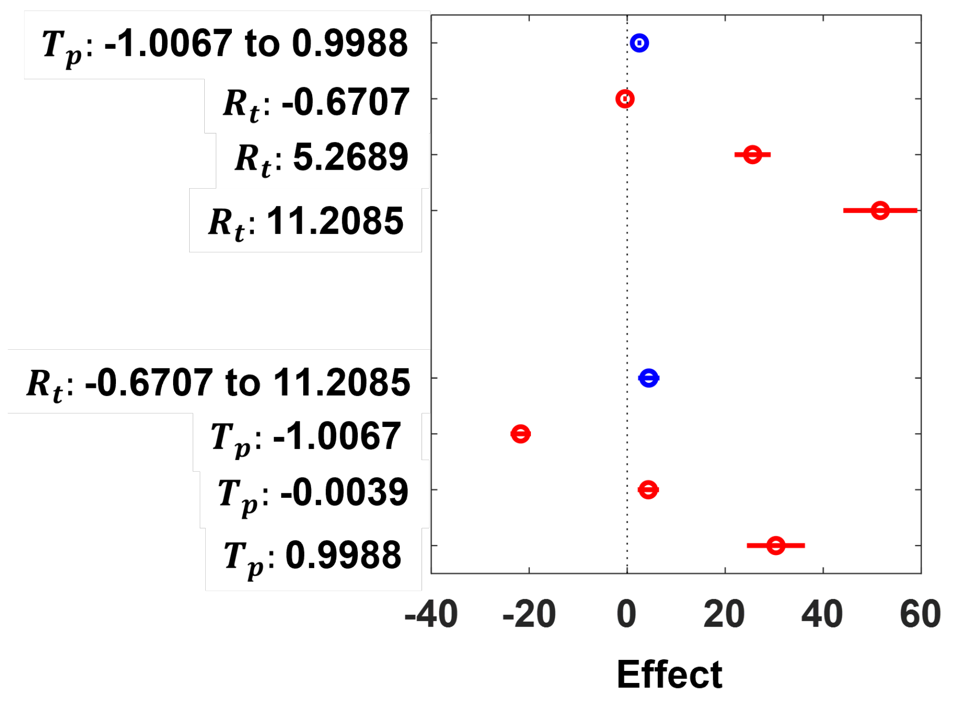
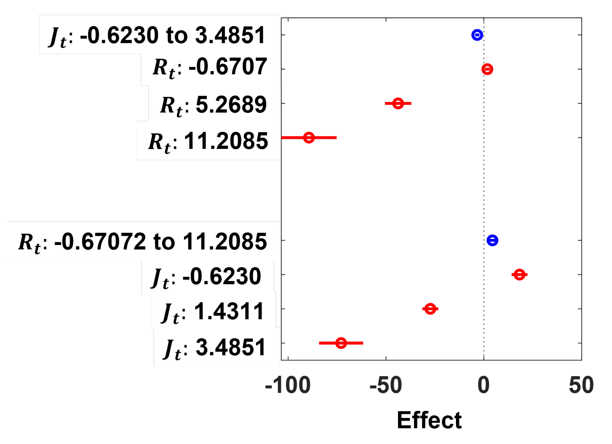
5.3. Pairwise Covariances and Correlations of the SDN Parameters
To have the measures that indicate the extent to which the SDN performance metrics (i.e.,
,
and
) change in tandem (alongside each other), their pairwise covariances are derived to have the covariance matrices reported in
Table 5,
Table 6 and
Table 7. A measure of covariance between any two observations (
and
) in the dataset of the SDN performance metrics can be described mathematically as follows:
where
n is the total number of observations in the dataset,
i is the
ith observation in the dataset,
is the mean of all observations for
X and
is the mean of all observations for
Y such that:
where
and
are the variances of all observations for
X and
Y, respectively.
From
Table 5, the following inferences can be drawn for
: (1) The covariances between the
metrics for the paired SDN scenarios are mostly close to or approaching zero. This suggests that the paired values of the
metrics may vary independently of each other for these paired SDN scenarios, except for when the SDN is subjected to TCP flooding attack and HTTP flooding attack. This corroborates the analysis of the distributions of
discussed in
Section 5.2. (2) The large positive covariance between the
metrics for when the SDN is subjected to TCP flooding attack and HTTP flooding attack indicates that, when the
metric resulting from subjecting the SDN to TCP flooding attack is above its mean, the
metric from subjecting the SDN to HTTP flooding attack will probably also be above its mean, and vice versa. In other words, the paired values of the
metric for both scenarios tend to increase together.
From
Table 6, the following inferences can be drawn for
: (1) The covariances between the
metrics for the SDN scenarios are mostly close to or approaching zero. This suggests that the paired values for
metrics may vary independently of each other for the paired SDN scenarios. This corroborates the analysis of the distributions of
discussed in
Section 5.2. (2) The negative covariances between the
metrics when the SDN is subjected to UDP flooding attack and when it is operating normally or subjected to TCP flooding attack or subjected to HTTP flooding attack indicate that, when the
metric is above its mean in any one of these paired SDN scenarios, it is probably below its mean in any one of the other SDN scenarios in the same pair. In other words, an inverse relationship exists between the
metrics for these paired SDN scenarios. Note that, since the negative covariances are close to or approaching zero, the first inference could be a better generalized inferential assessment.
From
Table 7, the following inferences can be drawn for
: (1) The covariances between the
metrics for the paired SDN scenarios are mostly positive and negative. This suggests the that
metrics for these paired SDN scenarios tend to be either above or below their means. (2) The approximately null covariance between the
metrics for when the SDN is operating normally and, when it is subjected to HTTP flooding attack, suggests that the paired values of the
metrics may vary independently of each other. (3) The positive covariance between the
metrics when the SDN is subjected to UDP flooding attack and when it is subjected to HTTP flooding or operating normally suggests that, when the
metric is above its mean in any one of these paired SDN scenarios, it is probably above its mean in any one of the other SDN scenarios in the same pair. In other words, the paired values of the
metrics increase together for these paired SDN scenarios. (4) The negative covariance between the
metrics when the SDN is subjected to TCP flooding attack and when it is operating normally or subjected to UDP flooding attack or subjected to HTTP flooding attack indicates that, when the
metric is above its mean in any one of these paired SDN scenarios, it is probably below its mean in any one of the other SDN scenarios in the same pair. In other words, an inverse relationship exists between the
metrics for these paired SDN scenarios.
Covariances tend to be difficult to interpret, so measures of correlations are often required for more robust analysis [
26]. For example, covariances close to or approaching null for
and
indicates that
and
vary independently of each other. This can be observed in
Table 5,
Table 6 and
Table 7 for
,
and
, respectively. In a technical sense, independence implies correlation, but the converse or reverse is not necessarily true. To have a scaled form of the covariance measures reported in
Table 5,
Table 6 and
Table 7, pairwise correlation measures that represent how strongly the SDN performance metrics are related to each other are derived to have the correlation matrix reported in
Table 8,
Table 9 and
Table 10. A measure of correlation between any two sets of observations (
X and
Y) in the dataset of the SDN performance metrics can be described mathematically as follows:
From
Table 8, the following inferences can be drawn for
: (1) The correlations between the
metrics are mostly positive and approaching null, indicating that some linear positive relationships exist between the
metrics for the SDN scenarios, but they are not necessarily strong. (2) A perfect positive linear correlation exists between the
metrics for when the SDN is operating normally and when it is subjected to UDP flooding attack. This corroborates the analysis of the distributions of
metrics discussed in
Section 5.2. (3) A strong positive linear correlation exists between the
metrics for when the SDN is subjected to HTTP flooding attack and when it is subjected to UDP flooding attack. This also corroborates the analysis of the distributions of
metrics discussed in
Section 5.2. (4) Negative linear correlations exist between the
metrics for when the SDN is operating normally and when it is subjected to HTTP flooding, and for when the SDN is subjected to UDP flooding attack and HTTP flooding attack.
From
Table 9, the following inferences can be drawn for
: (1) The correlations between the
metrics are mostly positive and unity, indicating that perfect linear positive relationships exist between the
metrics for the SDN scenarios. (2) Some of the correlations between the
metrics are negative and approaching null, indicating that some negative linear positive relationships exist between the
metrics for the SDN scenarios, but they are not necessarily strong. (3) Perfect positive linear correlations exist between the
metrics for when the SDN is operating normally and when it is subjected to TCP flooding attack or HTTP flooding attack, and for when the SDN is subjected to TCP flooding attack and HTTP flooding attack. This corroborates the analysis of the
metrics carried out earlier. (4) Negative linear correlations exist between the
metrics for when the SDN is operating normally and when it is subjected to UDP flooding attack, and for when the SDN is subjected to UDP flooding attack and TCP flooding attack or HTTP flooding attack. This also corroborates the analysis of distributions of the
metrics discussed in
Section 5.2.
From
Table 10, the following inferences can be drawn for
: (1) Some of the correlations between the
metrics are positive and approaching null, indicating that some linear positive relationships exist between the
metrics for the SDN scenarios, but they are not necessarily strong. (2) Some of correlations between the
metrics are negative, indicating that some negative linear positive relationships exist between the
metrics for the SDN scenarios. (3) Significant positive linear correlations exist between the
metrics for when the SDN is operating normally and when it is subjected to UDP flooding attack. This corroborates the analysis of the distributions of
metrics discussed in
Section 5.2. (4) Significant negative linear correlations exist between the
metrics for when the SDN is operating normally and when it is subjected to TCP flooding attack, and for when the SDN is subjected to TCP flooding attack and when it is subjected to UDP flooding attack or HTTP flooding attack. This also corroborates the analysis of the distributions of
metrics discussed in
Section 5.2.
The single run of the EDA implementation costs about 3.2 s in total on the workstation mentioned above. Thus, it can be said, in practice, a suitable augmentation of the EDA process that features as a complementary add-on or toolbox to existing SDN monitoring and evaluation software will likely offer a promising data analytic framework for real-time trend analysis, pattern recognition and overall monitoring and evaluation of SDN traffic and performance metrics to an order of less than 5 s on conventional workstations, for every 15-min samples of SDN data collected. This time window is sufficient and reasonably short, and it will ultimately reduce the current average time required to respond to potential attacks on real-world SDNs because inferences can be made in a shorter time.


