
Calculating the Segmented Helix Formed by Repetitions of Identical Subunits thereby Generating a Zoo of Platonic Helices †


Public Invention, 1709 Norris Dr., Austin, TX 78704, USA
†
This paper is an extended version of our paper published in Proceedings of the IMA Conference on Mathematics of Robotics, Manchester, UK, 9–11 September 2020; Springer: Cham, Switzerland, 2020; pp. 115–124.
Mathematics 2022, 10(14), 2533; https://0-doi-org.brum.beds.ac.uk/10.3390/math10142533
Submission received: 29 June 2022
/
Revised: 14 July 2022
/
Accepted: 16 July 2022
/
Published: 21 July 2022
Abstract
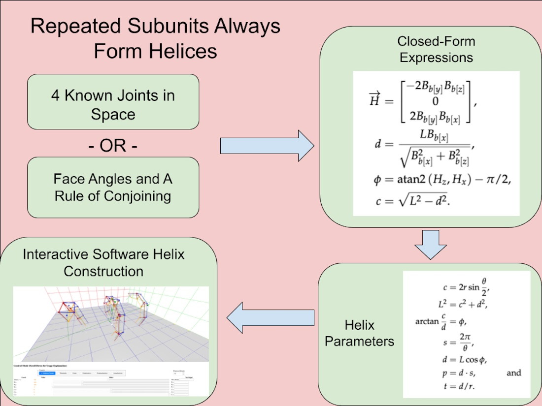
:Eric Lord has observed: “In nature, helical structures arise when identical structural subunits combine sequentially, the orientational and translational relation between each unit and its predecessor remaining constant.” This paper proves Lord’s observation. Constant-time algorithms are given for the segmented helix generated from the intrinsic properties of a stacked object and its conjoining rule. Standard results from screw theory and previous work are combined with corollaries of Lord’s observation to allow calculations of segmented helices from either transformation matrices or four known consecutive points. The construction of these from the intrinsic properties of the rule for conjoining repeated subunits of arbitrary shape is provided, allowing the complete parameters describing the unique segmented helix generated by arbitrary stackings to be easily calculated. Free/Libre open-source interactive software and a website which performs this computation for arbitrary prisms along with interactive 3D visualization is provided. We prove that any subunit can produce a toroid-like helix or a maximally-extended helix, forming a continuous spectrum based on joint-face normal twist. This software, website and paper, taken together, compute, render, and catalog an exhaustive “zoo” of 28 uniquely-shaped platonic helices, such as the Boerdijk–Coxeter tetrahelix and various species of helices formed from dodecahedra.
Keywords:
solid geometry; helix; Chasles’ theorem; platonic helix; tetrahelix; linear algebra; computer graphicsMSC:
51N20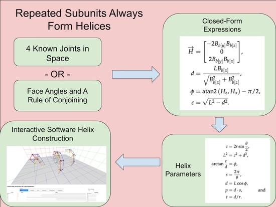
1. Introduction
During the Public Invention Mathathon of 2018 [1], software was created to view chains of regular tetrahedra joined face-to-face. The participants noticed whenever the rules defining the face to which to add the next tetrahedron to were periodic, the resulting structure was always a discrete helix.
Although unknown at that time, this is a consequence of:
Observation 1
(Lord’s observation). “In nature, helical structures arise when identical structural subunits combine sequentially, the orientational and translational relation between each unit and its predecessor remaining constant.” [2]
Although fairly obvious in hindsight from screw theory, we have found no articulation of this statement in writing, so feel justified in naming it after the author of its earliest statement. The surprising fact that DNA is a double helix allows replication and RNA synthesis by the unzipping and rezipping of the helix. However, the fact that it is helical in nature is unsurprising, since it follows directly from Observation 1 and the fact that the strands of DNA are formed of repeated chemical units of approximately the same shape arranged sequentially.
The purpose of this paper is to prove Observation 1 and provide mathematical tools and software for studying arbitrary segmented helices generated in this way.
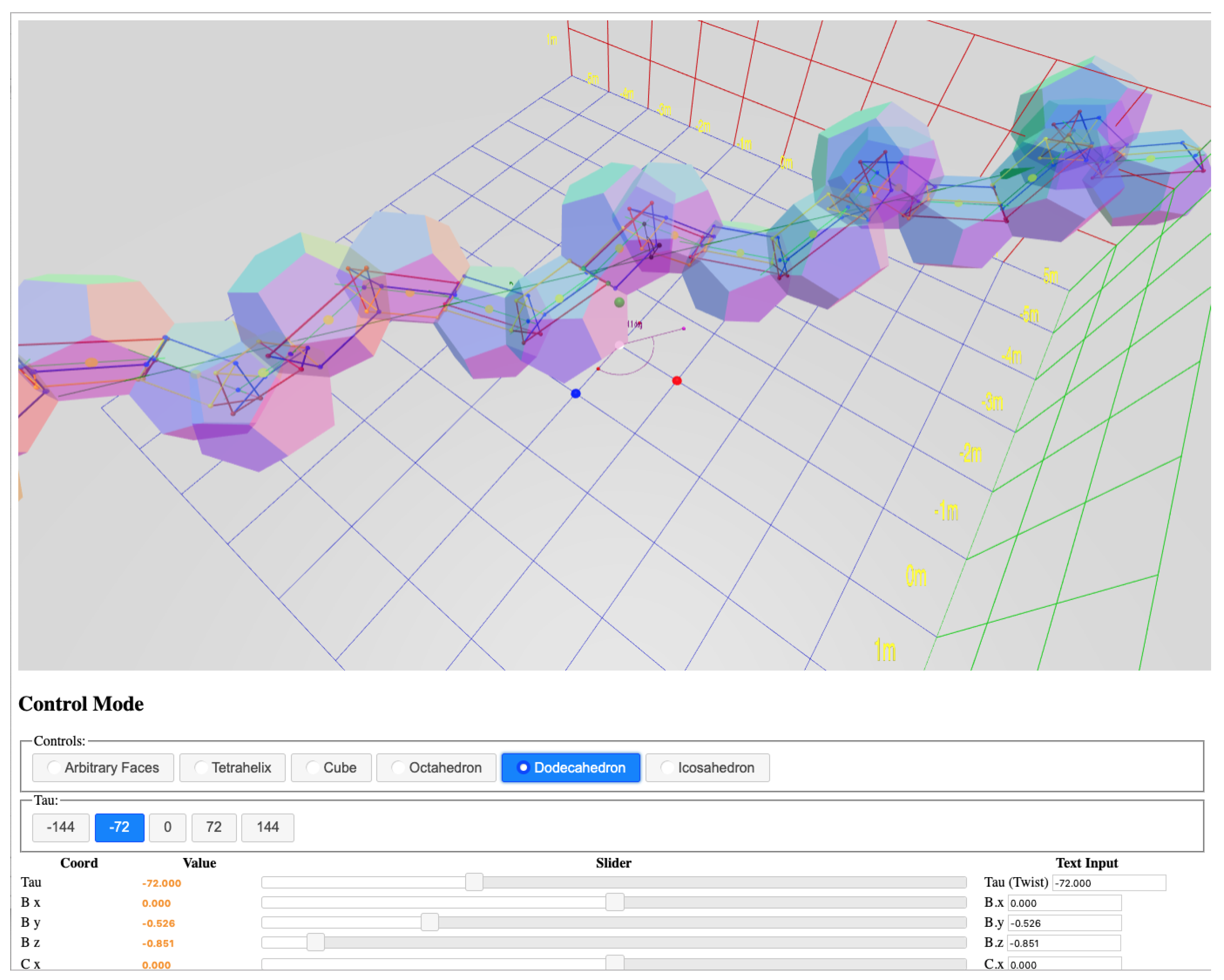
Finding the properties of a segmented helix from three contiguous segments on the helix from screw theory [3,4,5,6], is explained and formulated. An interactive, 3D rendering website written in JavaScript [7] which allows both calculation and interactive play and study is provided [8] (see Figure 1). This allows a structure, or “molecule”, coincident to a segmented helix to be designed by adjustments to the repeated object, or for the shape of a repeated subunit to be inferred from the intrinsic properties of the segmented helix. Kahn’s method of helix fitting [5,9,10] is modified to cover some degenerate situations.
We exploit Lord’s observation to discover symmetry which allows us to compute the helix when subunits are joined face-to-face with the same twist. Kahn was investigating proteins, which do not have faces, but geometric solids and other macroscopic solid objects do. This concept can be generalized to a joint face angle, even if the objects conjoined do not technically have flat faces. This symmetry allows us to compute the parameters of the segmented helix purely from properties intrinsic to a single object and the joining rule. We prove that varying the twist of the joint faces through a complete rotation produces a smoothly varying spectrum of shapes that always includes a torus-like shape and a zig-zag planar segmented helix of maximal extent. Finally, as an important demonstration, these tools are used to produce a catalog of all possible helices generated by vertex-matched face-to-face joints of the Platonic solids, of which only the tetrahelix [11,12,13,14,15] has been completely described to date. This paper extends a very abbreviated conference paper which did not include the catalog of Platonic solids or all the calculations in Section 2.3 and Section 2.6, nor the proofs of Theorem 4 [16].
1.1. A Warm-Up: Two Dimensions
Considering the problem in two dimensions may be a valuable introduction. Suppose a polygon has two edges, called A and B, and the length L of the polygon is defined as the distance between the midpoints of these edges. Suppose these polygons are only joined by aligning A of one polygon to B of another polygon, with their midpoints coincident. Further, assume that inversions of the polygon are disallowed. Imagine there exists a countable number of polygons indexed from 0. Then what shapes can be made by chaining these polygons together?
Theorem 1.
When polygonal subunits are conjoined with their axes at angle θ, they form a circle of radius:
where if the circle is of infinite radius, that is, a straight line.
Proof.
Each joint between polygons and will place the axes of the polygons at the same angle, , since these polygons do not change shape. Define to be positive if we move anti-clockwise from to and negative if we move clockwise. If , the joints will be collinear.
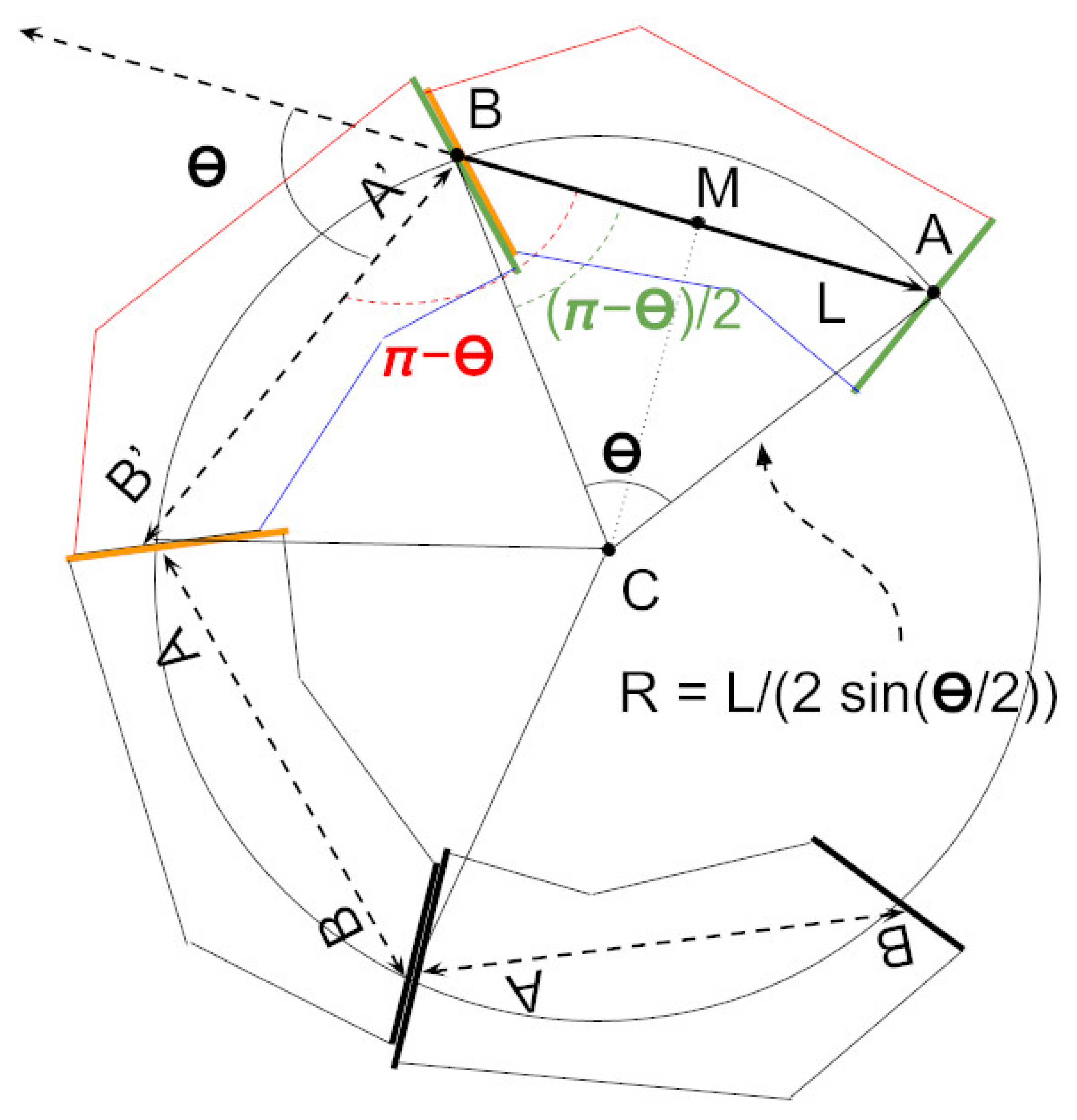
If , then form an isosceles triangle in the direction of the second object, whose axis is . Form this triangle so that one edge is a bisector of the angle between the axes , as illustrated in Figure 2. Make .
Becuase is a bisector of , . Therefore . By considering the right triangle formed by midpoint M of and C, the length of the sides can be computed by the half-angle of theta:
Since the triangles formed by placing a new object are similar and share a side which is an angle bisector, they all share the point C. Therefore, the axis points A and B for each object lies on a circle of radius R with center C. □
1.2. The Segmented Helix
An analogous result holds in three dimensions.
Such a helix has a radius of r and slope (if ) of . The pitch of the helix—the change in t needed to make one complete revolution—is . Note that a helix may be degenerate in two ways. If , these equations become a line. If , these equations describe a circle in the -plane. If and , the figure is a point.
Such helices are continuous, but it is stacks of discrete objects under investigation. A goal is to derive the parameters for a continuous helix from such discrete objects by studying a helix evaluated at integral points. Call such an object a segmented helix. A segmented helix may be thought of as function that, given an integer, gives back a point in 3-space,
where d is the distance or travel along the helix axis between adjacent joints. In this canonical representation the helix axis is the z-axis. is the rotation around the z-axis between adjacent points. r is the radius of the segmented helix. Note that if , a third form of degeneracy (to the human eye) occurs: that of a segmented helix which is a zig-zag contained completely within a single plane.
If one thinks of the segmented helix as describing a polyline in 3-space, the properties of that polyline are of interest. Considering only the intrinsic shape of the segmented helix that are independent of position and orientation in space, there are three degrees of freedom: and .
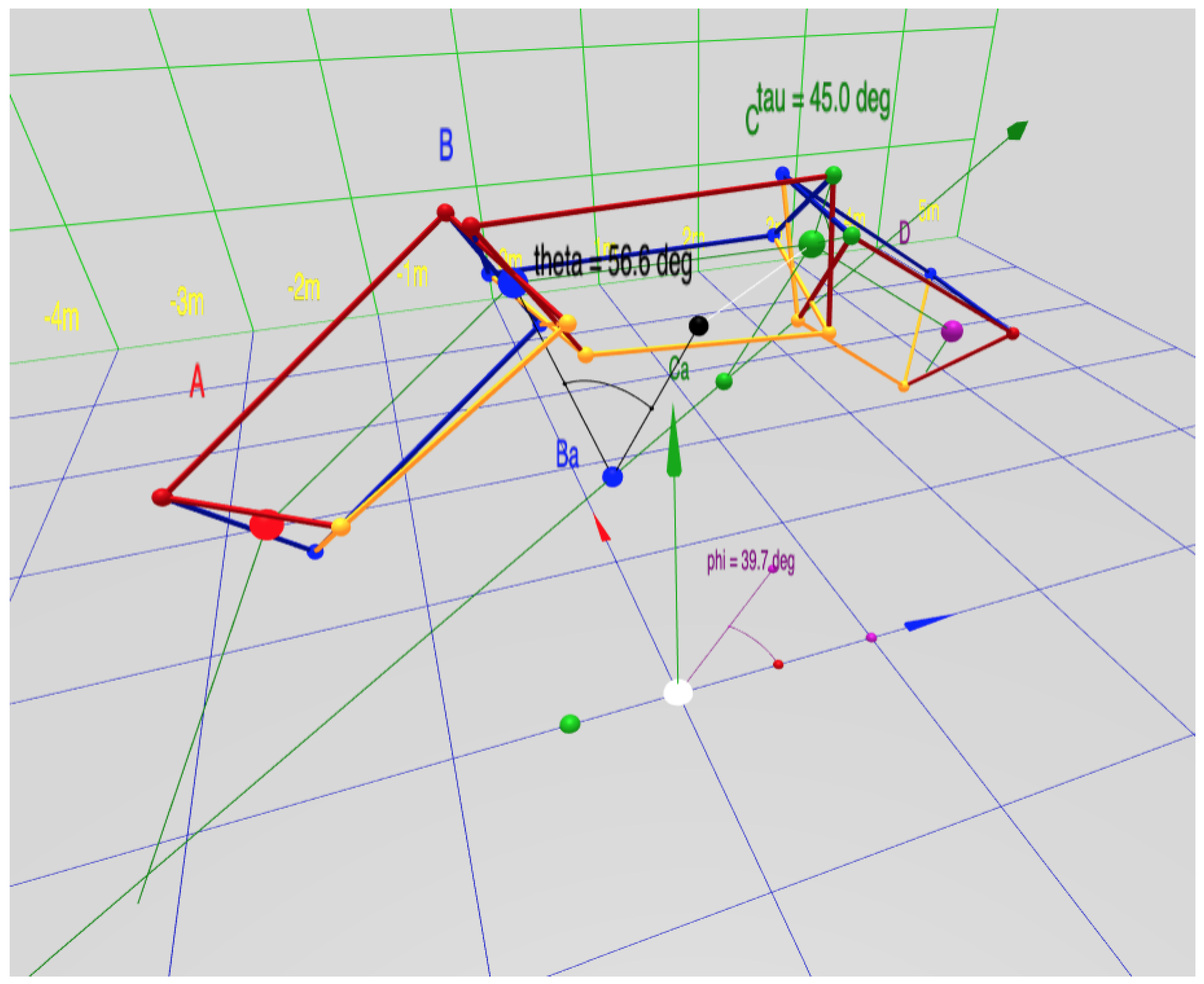
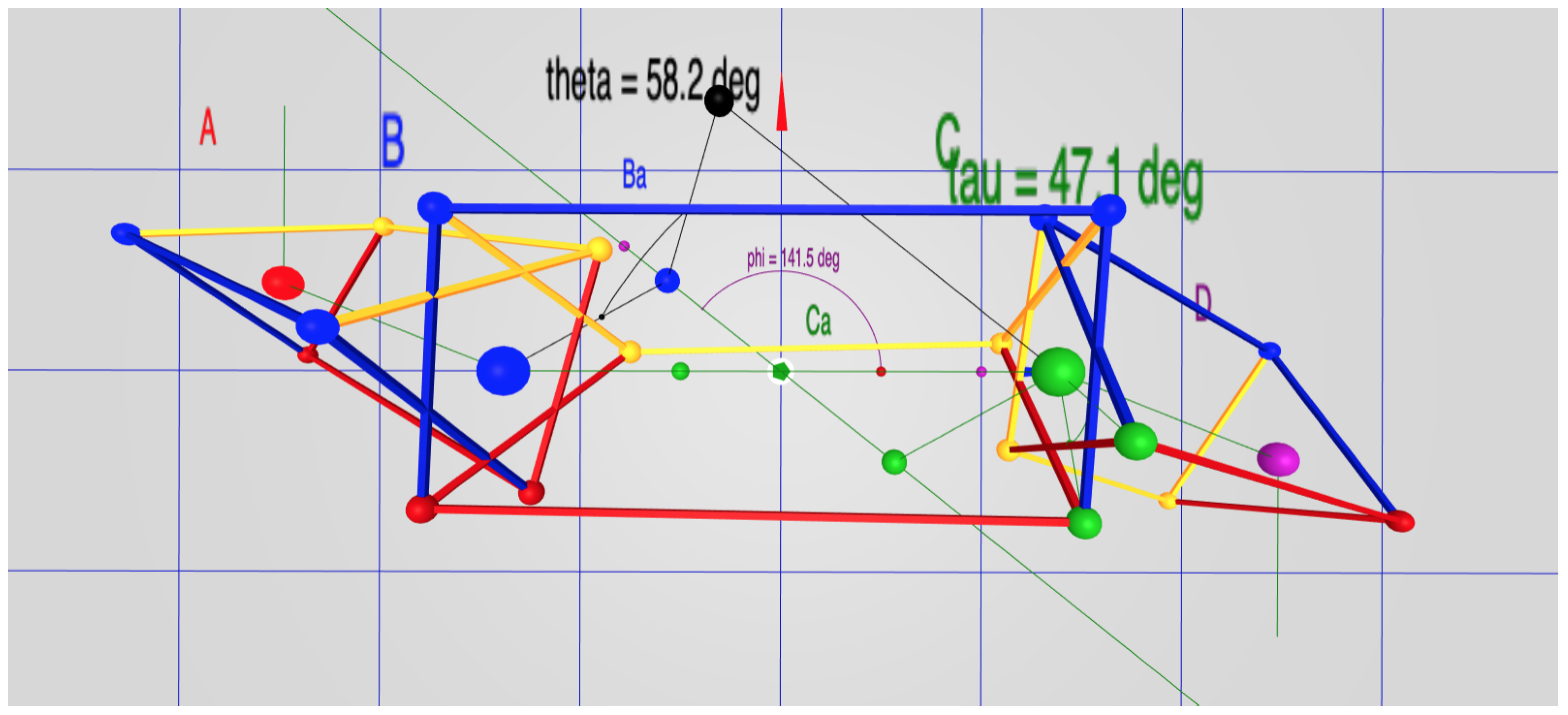
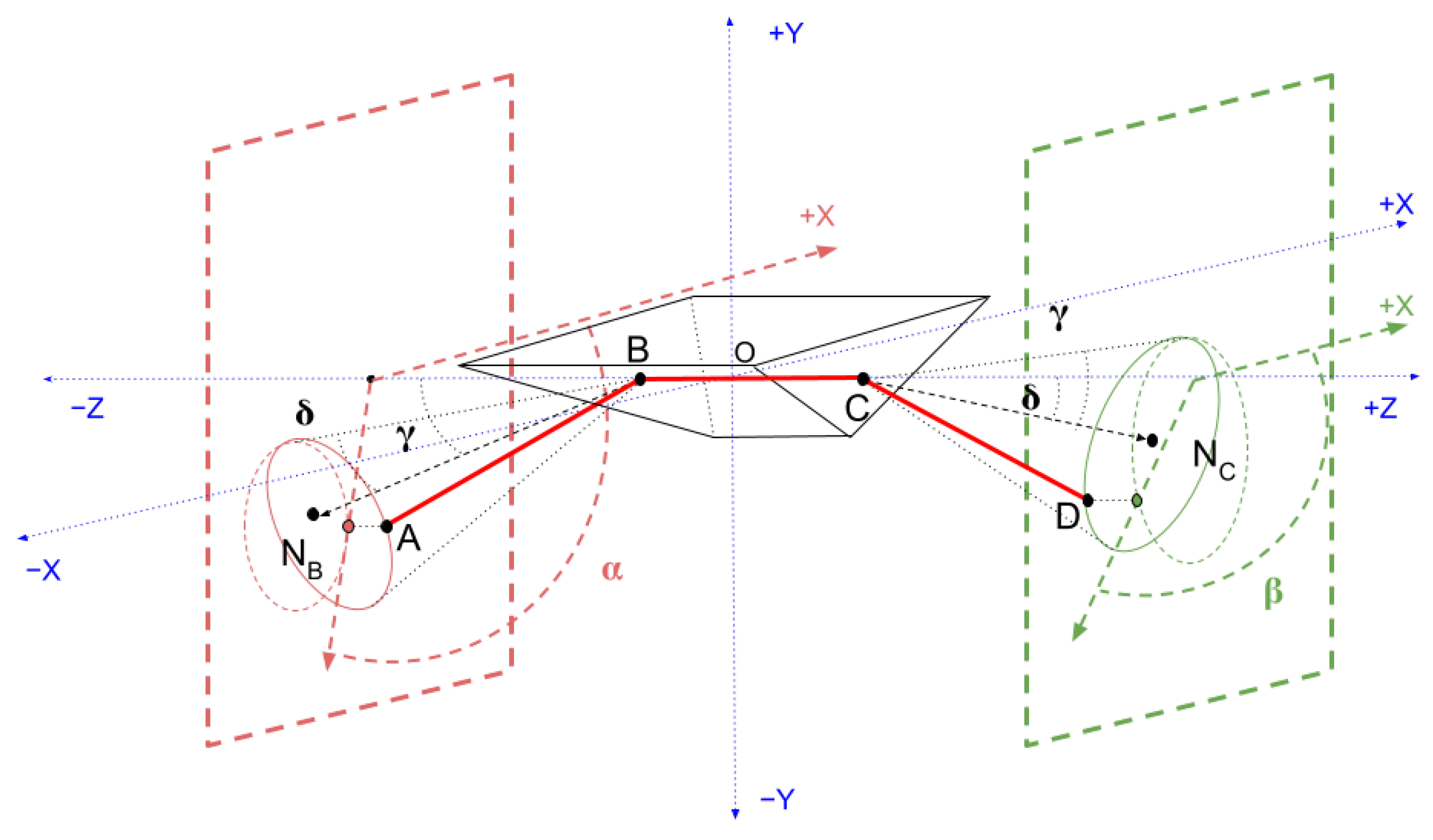
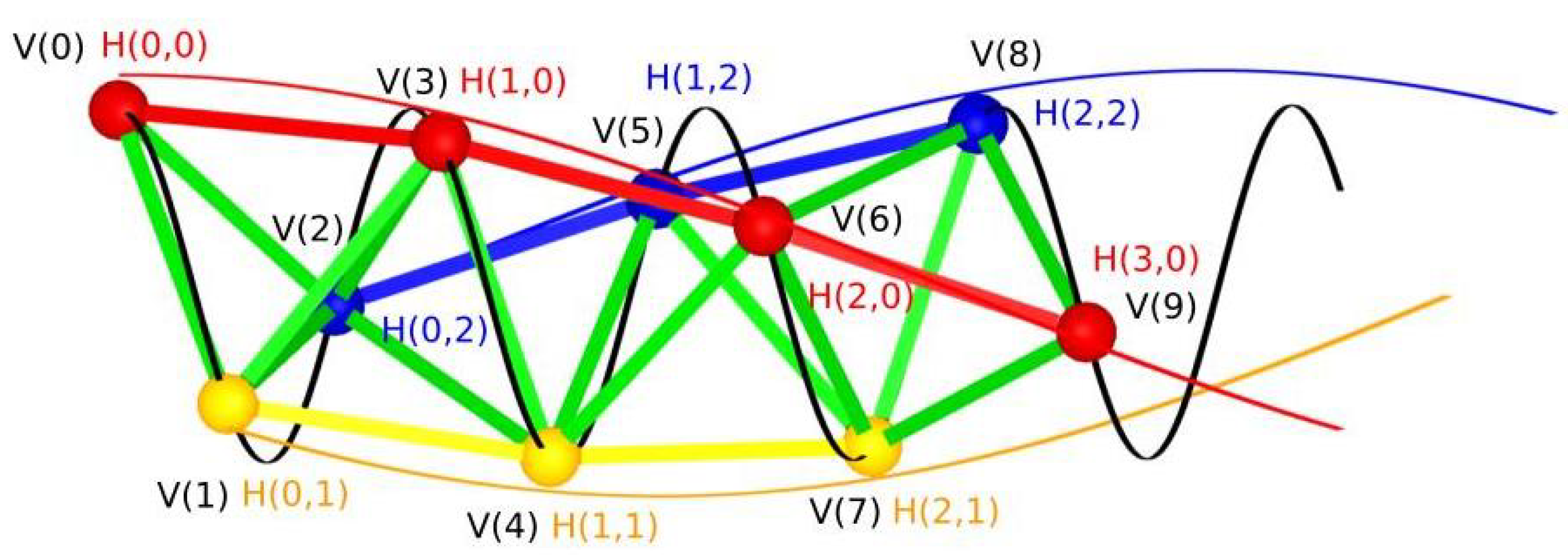
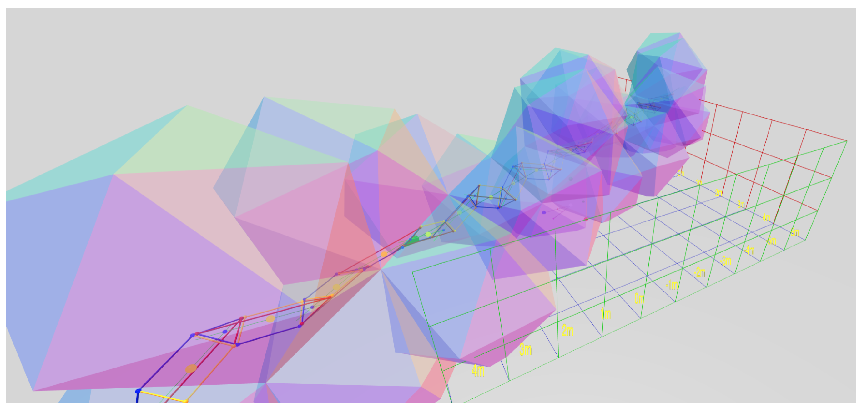
Figure 3 demonstrates naming convention concepts. It is a screenshot taken from the real-time interactive website [8]. The software allows parallax by supporting interactive rotation, which makes the 3D structure easier to perceive; please visit the interactive page during this discussion of naming conventions.
In Figure 3, and the website, we represent the object as a prism with a triangular cross-section, because this is the simplest physically realizable macroscopic object that supports a face-to-face connection. In this diagram, the points , and D are represented by the sphere of the same color as the label. The view is roughly in the direction of the axis of the segmented helix, which is drawn as a dark green arrow, pointing in the positive z and positive x direction, parallel to the -plane. For ease of viewing, the entire segmented helix has been raised by two units on the y axis. The segment has coordinate , is aligned with the z-axis, and is centered in the z direction.
The positive and z axes are shown by the red, green, and blue axis arrows, respectively. Following the computer graphics convention, the y axis is oriented vertically. The points , and D correspond to , and , respectively, for a segmented helix aligned to the raised axis (not the z-axis). A thin green polyline represents the segmented helix, and thus connects the joints , and D. The points are wrapping around the axis clockwise, with an angle of as shown by the on-screen protractor as the rotation from one point to the next. As will be explained in Section 2.15, is the face-on-face joint rotation, in this case of 45°. The helix angle is rendered by a protractor on the plane; this is the angle between the axis of the helix and the z axis, and therefore the angle of any one segment against the helix axis.
Any point on the segmented helix has a closest point on the axis of the helix. In particular, the points closest to the joints are called joint axis points. Then d is the distance along the axis between consecutive joint axis points.
A line is drawn from the blue point B to a black sphere on the helix axis, the joint axis point, denoted . Analogously, is the point on the axis closest to the green point C.
A segmented helix located in space is completely determined by the parameters , a vector describing the axis of the helix, and the position of any one joint.
Because the segmented helix is a discrete structure, one can reframe the concept of pitch as sidedness s: how many segments (sides) make a complete rotation?
The following concepts and conventional variable names for them will be related:
- L is the distance between any two adjacent joints (between B and C, for example).
- r is the distance between a joint and the helix axis (between B and for example).
- is the rotation about the helix axis between two consecutive joints.
- c is the length of a chord formed by the projection of the segment between two points projected along the axis of the segmented helix (a chemist may recognize this as the distance between residues on a helical wheel projection).
- d is the distance along the axis of the helix between any two joint axis points (between and in Figure 3, for example, rendered as a small black and blue sphere, respectively).
- is the angle between any vector between two adjacent joints and the axis of the helix. In physical screws used in mechanical engineering, this is analogous to the helix angle [18].
- p is the pitch of the helix, the distance traveled in one complete rotation.
- s is the number of segments in a complete rotation (in general not rational).
- Finally, we find it useful to define the tightness of a segmented helix as travel divided by radius, a number analogous to the extension of a coil spring or slinky. A torus-like segmented helix has zero tightness and a zig-zag has maximum tightness. The letter t represents tightness.
These quantities are related:
Measuring demands a decision on the sign of the direction of the axis, which is arbitrary and not based on the physical shape.
Section 2.3, Section 2.6 and Section 2.15 relate these properties to properties intrinsic to the joint or interface between two segments or objects in the segmented helix.
1.3. Sign Conventions for Spatially Located Segmented Helices
When thinking about the overall shape of a segmented helix, one is likely to be interested in the absolute magnitude of its intrinsic properties.
However, when doing computer graphics work or kinematic calculations, the sign conventions are critical. Because this paper wishes to emphasize the continuum of shapes produced by changing an object used to generate the segmented helix, and, in particular, is interested in the degenerate helix which produces toroidal figures, it is preferable to be able to discuss the axis of a segmented helix as existing even when the figure has no travel along the axis (that is, when ).
Therefore adopt the following conventions:
- A right-handed coordinate system.
- The helix axis is a normalized vector which never vanishes.
- The travel along the axis (d) is negative when the helix is anti-clockwise (that is, when motion from joint n to joint appears anti-clockwise when , zero when toroidal), and positive when the helix is clockwise.
- is never negative.
2. Results
2.1. The Intrinsic Properties of Periodic Chains of Solids
Although fairly obvious from Chasles’ Theorem, in order to prove Observation 1, additional clarification is helpful. If chains of identical repeated 3D units are conjoined identically, they are periodic chains, and they generate a segmented helix coincident on their joints. Identical objects conjoined via a rule produce periodic chains of objects that are uniformly intersected by segmented helices and may be degenerate in one of three ways that might not strike the human eye as a helix at first glance:
- (1)
- The segments may form a straight line. (For example, see Figure 14).
- (2)
- The segments may be planar about a center, forming a polygon or ring. (For example, see Figure 20).
- (3)
- The segments may form a planar saw-tooth or zig-zag pattern of indefinite extent (For example, see Figure 4).
There are two complementary ways of learning about such segmented helices. In one approach, we may have knowledge of the segmented helix and wish to learn about the subunits and the rule with which the subunits are combined. For example, we may have microscopic objects such as proteins or atoms, and we know from crystallography something about the positioning of these objects, without knowing ahead of time the angles at which these objects would combine in their natural environment. In this case, we use a variant of a linear algebra method [5] for determining the radius, travel, and “twist” of the segmented helix (twist will be defined precisely below).
In the other approach, one may know a priori exactly the relevant properties of the objects and the rule with which they combine and seek to compactly describe the segmented helix they create. For example, a mathematician may consider a chain of dodecahedra, or a woodworker may cut identical flat-faced chunks of maple wood, which are to be glued together face-to-face. In these cases, everything about the objects and the rules for conjoining is known before the first two objects are glued together. Call this the joint face normal method, because it can be simulated by joining two flat faces together with a specified twist, even if the objects in question do not actually have a physical face (such as molecules).
In both cases, it is useful to understand how a change in a face normal or a twist affects the parameters of the segmented helix, and, conversely, useful to be able to choose the construction of the subunits to achieve a particular segmented helix.
In engineering, sometimes the term special helix [19] is used for helical curves on non-cylindrical surfaces. This paper uses the term helix only in the sense of cylindrical helix.
2.2. Periodic Chains Produce Segmented Helices
A periodic chain is, in fact, a simple object which demonstrates tremendous symmetry. Before using this symmetry in the construction of the segmented helix corresponding to a periodic chain, it is valuable to prove that such a segmented helix indeed exists for every periodic chain. Because periodic chains are merely a clarification of the “identical structural subunits” of Observation 1, this theorem proves that observation.
Theorem 2
(Segmented Helix). Consider N identical objects which each have two points, A and B, called joints. Call the axis of this object. Consider the frame of reference for this object to have its axis on the z-axis with B in the positive direction, the midpoint of the object being at the origin.
Consider any rule that conjoins A of the object to B such that from the frame of reference of i, the object and anything rigidly attached to it is always in the same position in the frame of reference for i. Informally, “looks the same” to i, no matter what i is chosen, . Call a chain of N identical rigid objects conjoined via a rule that conjoins to in such a way that every vector rigidly attached to object is always in the same position relative to the frame of reference constructed from object i, a periodic chain.
Any periodic chain of three or more objects has a unique segmented helix whose segments correspond to the axes of these objects.
Proof.
By induction.
Base Case ():
Take an object A with axis . By Chasles’ theorem [20] there is a screw axis , a set of rotations, and a transposition d which moves the first object to the position where the second object B with axis is. Take one of the rotation angles of smallest value. Construct the points , and as the closest points to and C on this screw axis. These points are collinear by construction.
Now add the object to object by the rule of periodic chains. Consider the points and from A’s frame of reference. Let . Construct the point on the screw axis as the point closest to D on that line.
Because in object B’s frame ofreference must look like in A’s frame of reference, the distance . From A’s frame of reference, are collinear, so the points must be collinear in B’s frame of reference.
In any frame of reference, if are collinear and are collinear, then are collinear.
Now, looking backward from towards A, the length must be the same as the length so as to not violate the rule. So . Similarly let . Then by construction. By the rule of conjoining, the vector is a rigid transformation of , so . By symmetry, . Compute as the rotation about that takes into . By the rule of attachment, also takes into and into .
Next, construct a segmented helix, of radius r, distance d, and angle . The segmented helix axis and joints can be positioned coincident with the screw axis so that . Then , , and .
Therefore, for the base case of three objects, there is a segmented helix whose segments coincide with the axes of the objects.
Inductive Case ():
Assume there is a segmented helix coinciding with the first k objects, and consider the frame of reference of the kth object. The axis and any other rigid property of the th object stands in relation to object k as k stood to .
By the assumption of induction, the kth object has an axis coincident to a segment of a segmented helix. Attach vectors and from the joints of object k to the corresponding axis joints of the segmented helix perpendicularly. Define these vectors in the frame of reference for k.
To the th object, the tips of and vectors ( and ) define a line segment which lies on the axis of the segmented helix H, with the tip of coincident with the tip of .
By the rule of conjoining and by induction, since this is true of the th object, it is true of the kth object. Therefore the tips of the th object’s attached vectors and form a vector which lies on the axis H, extending it in the same direction. The joint axis of the th object therefore coincides with the th segment of H.
Therefore, by induction, identical objects conjoined by the same rule always coincide with some segmented helix, whose parameters are discoverable. □
In engineering, the term helix angle refers to the angle between a line tangent to a continuous helix and the axis of the helix. In segmented helices, this is the same as the angle between the axis of each object in a periodic chain and the axis of the segmented helix coincident to it.
Consider objects which are, taken as individuals, highly asymmetric. For example, the B face does not have to be the same size as the A face. In fact, the object itself might be shaped like the letter “C”, and not completely enclose the axis. Taking the idea further, the object might be spiky, such as a stellated polyhedron or a sea urchin, and still be joined by joints relatively close to the center of the object. (This paper does not address the issue of self-collision of the objects, which would have to be considered if attempting to make a period chain of sea urchins).
It is perhaps not obvious that building a chain of such objects produces a segmented helix, and therefore that the helix angle is the same for each object, but this is a corollary of Theorem 2.
Corollary 1
(Segment Similarity). The helix angle of any object axis in a periodic chain is the same.
Proof.
The axes of each object coincide with a segment of a segmented helix. A segmented helix is completely symmetric no matter in which direction of the axis you look down or at which point on the axis you begin. The angle between each pair of objects is exactly the same. □
Corollary 1 will be used in the development of PointAxis algorithm, in the computation of segmented helix properties, to justify balancing face normals to produce an intrinsic out-vector, and to apply the PointAxis algorithm without actually assigning objects Cartesian coordinates.
2.3. Computing Screws and Segmented Helices from Transformation Matrices
The rule for how objects in a periodic chain are joined may be conveniently captured as a transformation matrix. In general, a human engineer will have to compute this transformation matrix from some other information, such as the face-to-face conjoining rule. We discuss how to do this from joint-face normal vectors in Section 2.15. However, a transformation matrix clearly captures the idea of repetition. Since by definition the objects in the chain are the same shape, moving one object into a new position and placing an identical copy of that object in that position are practically the same.
Using standard screw theory [3,6], a screw can be computed from such a transformation matrix. This consists of the axis of the screw , a point on the screw axis P, the rotation around the axis, and the transposition, or travel, along the axis of one transformation.
Neither a transformation matrix nor its corresponding screw transformation completely defines all of the intrinsic properties of a segmented helix. In particular, a matrix maps any point p to a point . Since this applies to all points no matter how far from the screw axis (axis of rotation), and such transformations preserve distance to this axis (the radius), the radius of a segmented helix is not determined by a transformation matrix or a screw. Since the helix angle changes with a radius for a helix of a given pitch, is not determined.
However, given a screw and one point on the axis of the screw fixing it in space and the location of one joint, all of the properties of the segmented helix are completely determined.
The software behind the interactive website implements the calculation of the screw directly from a transformation matrix, and the additional routines which determine all intrinsic properties from a joint position (making certain arbitrary alignment choices without loss of generality).
Although not original to this paper, it is difficult to find clear documentation on how to calculate the screw from the transformation matrix. We therefore include an exposition here, in the hope that it will be a useful and valuable addition to the code in the source code repository to a programmer seeking to duplicate this functionality.
2.4. Computing the Screw Axis from a Transformation Matrix
The goal is to compute a normalized vector aligned with the screw axis of the transformation composed and effected by a transformation matrix .
In order to be robust, it is valuable to check that the transformation matrix is a rigid transformation [21], as Chasles’ theorem applies only to rigid transformations. Transformation matrices in homogeneous coordinates, as typically used in kinematics and computer graphics, are convenient for this purpose, allowing the transformation represented by a matrix to be affected by simple multiplication.
The angle of rotation is computable from the trace of , :
Technically, arccos is multi-valued, but take to be in its principle range, . If is 0 or a multiple of , then we have the zig-zag degenerate case; the method of computing from the rotation basis of is numerically unstable. However, in this case we can compute the direction vector as the difference vector between an arbitrary point q (a 4 × 1 vector in homogeneous coordinates) and its transformation performed twice. Informally, this is a “zig, then a zag”:
(Note that in general is not normalized, . Additionally, recall that multiplication by a transformation matrix produces a point that is in a new position representing the transformation).
The variables and are primed to distinguish them from the symbols for the chord c and the travel along the axis d). The magnitude of , which vanishes when is 0 or multiple of , hence the need to treat those cases differently.
2.5. Combining a Single Joint with the Matrix
The vector gives the direction of the axis of the helix, but does not give a point that fixes it in space. Although the matrix in general produces both a rotation and a translation in space, the distance between q and in general depends on how far q is from the axis of rotation. If, however, we are given a single joint B in addition to , then we can completely determine the entire segmented helix. C is computed from :
Then d is computable as a projection:
These are the only properties that can be computed from the matrix alone, but given the length L along the object axis (not the helix axis) of an object the helix parameters are computable, based on relations already given in Section 1.2.
The chord of the segmented helix (that is, length of an object of axis length L projected along ) is:
Knowing the chord c and the amount of rotation allows us to compute the radius:
unless the chord is 0, in which case the radius is 0. The helix angle is a a function of c and d:
Sidedness and pitch (s and p) follow directly.
From these one may produce the joint axis point which is the point on the helix axis closest to B.
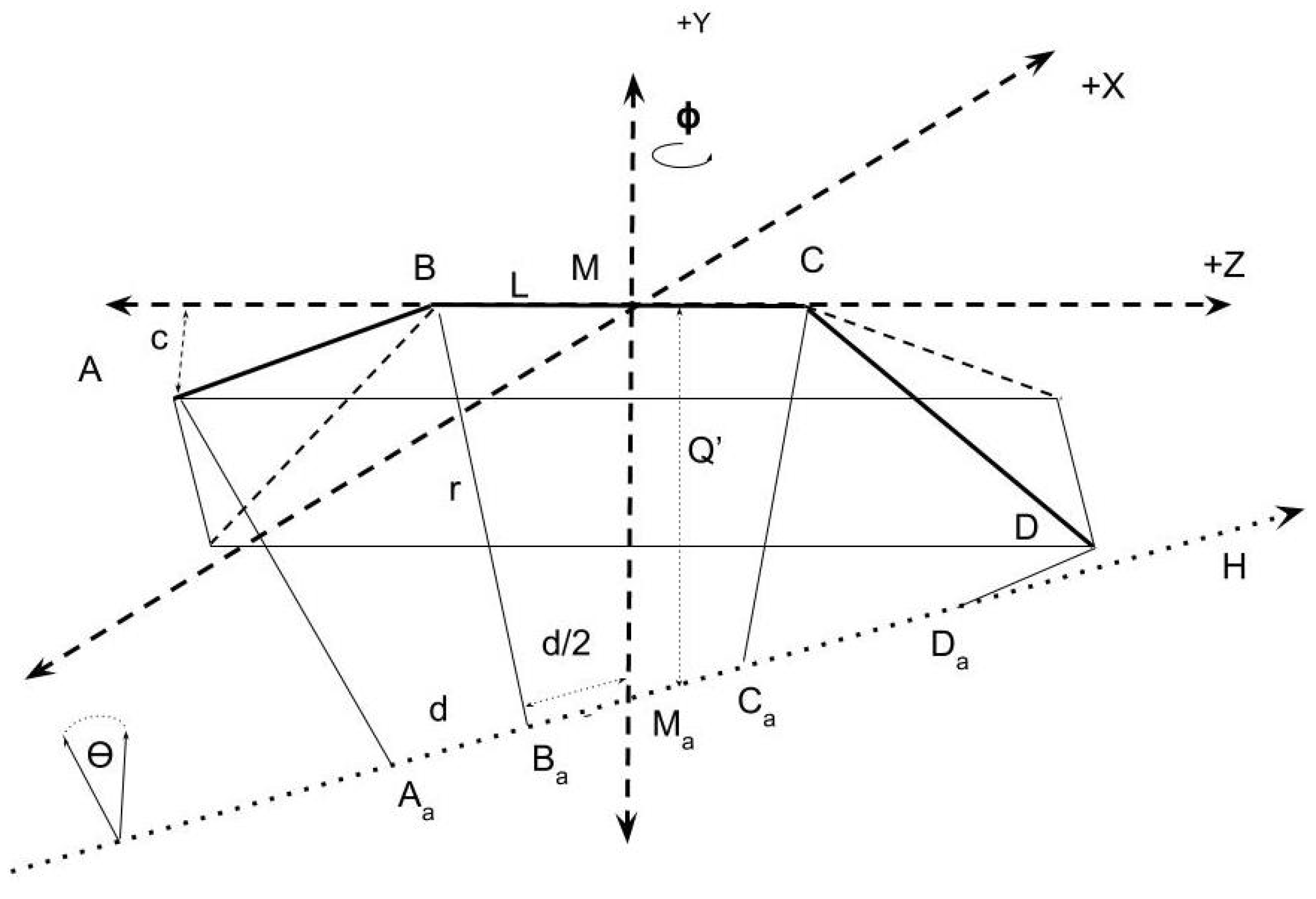
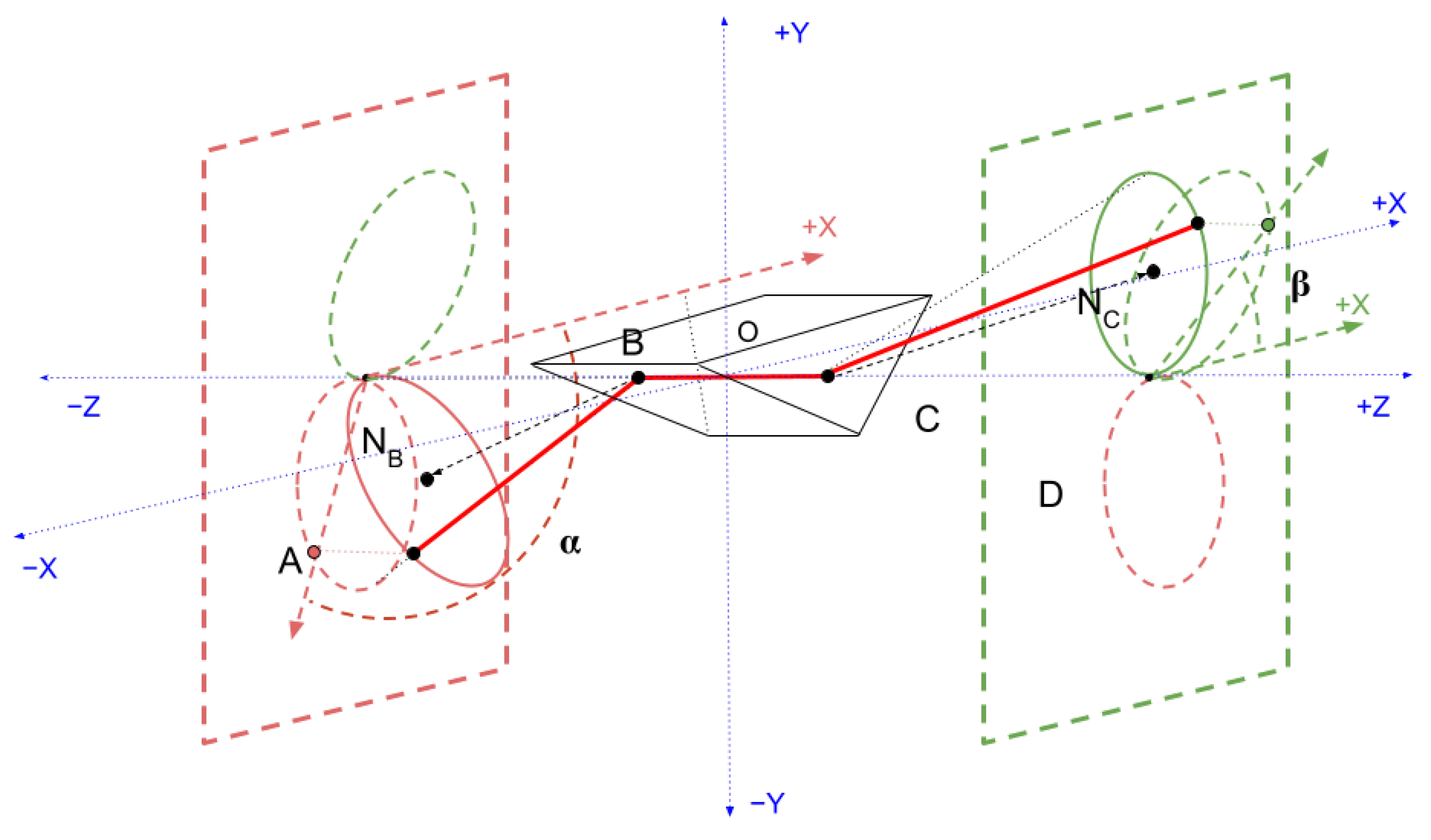
Figure 5 may be useful in picturing the following quantities. To do this, conceptually construct the midpoint, of and utilize the fact that the vector from to its closest point on the axis (call this vector ) is perpendicular to both and . Therefore, its direction is constructible via cross product, and its length l is computable from the radius and chord. is the midpoint of and , so just move back half the travel d along the vector H to get .
Thus, given only the transformation , the length L, and one joint B, one may compute all of the intrinsic properties () of the segmented helix and position it in space via and .
As is common in kinematics [23], there are many ways to represent the same physical or mathematical situation. Four consecutive joint positions also completely determine a segmented helix, as presented below. Because joints can be computed from transformation matrices and transformation matrices from joints, which method of calculation is preferable is largely a matter of choice and clarity. The code at the interactive website in fact codes both approaches and compares them as an automated test to ensure correctness.
A mechanical engineer, roboticist, or computer graphics expert is likely to find the computation from the transformation matrix more natural and convenient. A chemist or crystallographer is more likely to have learned the position of four points and wish to compute from that.
2.6. PointAxis: Computing Segmented Helices from Joints
Kahn [5] has given a method for computing the axis of a helix in the context of chemistry. This method uses the observation that the angle bisectors of the segments on a segmented helix are perpendicular to and intersect the axis of the helix. Because chemical helices may not be perfect and because the measurement of positions may not be perfectly accurate, it is common for chemists to use regression and fitting methods to fit helix parameters to observed positions on the helix. Kahn’s method was a prelude to some error-tolerant methods applicable to the realm of organic chemistry [9]. This paper is concerned only with pure geometry. Furthermore, Kahn was writing in 1989, and more convenient computing tools are now available. The algorithm presented, called PointAxis, here can be considered a modification of Kahn’s algorithm, which relies on the ability, working in the realm of pure geometry, to position the segments on the axes to simplify the derivation and computation.
2.7. A Sketch of the 4-Point Method
Using tools from linear algebra and well-documented algorithms, a sketch of finding the segmented helix from four consecutive known points , and D is:
- Construct a rigid transformation that places the points conveniently on the z-axis and balanced around the y-axis.
- Compute the bisectors of the angle between object axes , called and the bisecting angle of . If the points are collinear, they are a special case.
- Because these angle bisectors point at the axis of the segmented helix, their cross product is a vector in the direction of the axis. If and are parallel or anti-parallel the cross product is not defined and we have special cases.
- Otherwise the vectors and are skew, and the algorithm for the closest points on two skew lines provides two axis points and on these vectors which are the closest points on those lines and are also points on the helix axis.
- The distance between and B is the radius, and the distance between and is the travel d along the axis.
- The angle between and is .
2.8. Rotating into Balance from Face Normal Vectors
In order to use the PointAxis algorithm, we need a way to compute points A and D in balance around the axis .
Figure 6 shows a downward view of a balanced configuration (though raised above the origin instead of at the origin). A (the red sphere) is a reflection of D (the purple sphere) across the y-axis. Both A and D are hanging downward. If the structure were hung on a point at the origin, it would be physically balanced. As shown in the following, it is always possible to achieve this balance, even though a single object itself is not symmetric; in this figure, the normal of the B face is not symmetric with C face.
That this is always possible is important enough, if only for the convenience of calculation, that we consider it a Lemma:
Lemma 1
(Balance Lemma). For any segmented helix with selected consecutive joints and D, there is a rigid transformation that positions it such that:
- The segment is centered on the z-axis: .
- The joints A and D are in rotational balance about the y axis, as if they were weights hanging downward: and .
Proof Sketch of Lemma 1.
A key insight is that Theorem 2 implies that no matter how lopsided and different the normal vectors and for the joint faces are and no matter what we choose, the relationship of conjoined objects is always the same. After placing along the z-axis, there is always an angle which will rotate the points A and D into balance (that is, ).
The key to finding is to note that the projections of the B and C face normal vectors projected into the plane can be rotated so that they are balanced around the negative y unit vector. Such a projection into the cross-section of the helix is closely related to the helical wheel [24] plot in the study of alpha helices in proteins. Even if the lengths of the projections of the face normals in are different, this mechanism works, because by Observation 1 and Theorem 2, the points A and D must be symmetric about the segment .
By composing this balancing operation with the face-adjoining transformation matrix via adjoinPrism (see Section 2.16), A and D are placed in balance.
Note that in the zig-zag case, . □
The screw axis may now be computed from either the four points , and D or from the transformation matrix created to balance them.
2.9. On the Choice of the Screw Axis Direction
Given only a segmented helix without a position in space, the choice of direction for the axis is arbitrary. Changing the decision will make the screw axis point in the negative direction, change the sign of the travel d along the axis, and change to be .
As can be seen from interactive play with the website [8], it is entirely possible for the travel along the axis of the helix to be 0. In fact, choosing tends to produce toruses, which have no travel along the axis.
One could choose to represent this by making the unsigned length of the vector representing the axis be the length of the travel d. However, this would have the drawback that when d is zero it would be impossible to determine the axis of revolution of the torus. Although somewhat arbitrary, we have chosen instead to represent the axis as a normalized vector of unit length and to allow the travel to be negative. This has the benefit that changing through (something close to) zero smoothly changes d. However, it creates the problem that as approaches (something close to) from different directions the signs of the axes are different. That is, and describe exactly the same shape, but in our calculation, they will have different signs for the axes. The radius, pitch and absolute value of the travel, which are intrinsic to the shape, will be the same, but the axis vector, , and the sign of d will be different.
2.10. The 4-Point Method
Four consecutive points completely determine at least one segmented helix. Consider only the helix that makes the least rotation between these points, though more rapidly rotating helices will also intersect these points. The PointAxis algorithm takes four such points. Without loss of generality B and C are assumed to be centered on the z-axis, and that a rotation has been performed to balance A and D so that , and . Thus, the input to PointAxis in fact has only three degrees of freedom, which determine the three intrinsic properties which completely defines the shape of a segmented helix (but not its location in space).
In the derivations below, we rely on certain facts about the segmented helix formed by the stack of objects, the first of which is key:
- By virtue of Lemma 1, without loss of generality, think of any member whose faces and twist generate a non-degenerate helix as being “above” the axis of the helix. Furthermore choose to place the object in this figure so that , that is, that the members are symmetric about the z-axis. A and D are “balanced” across the -plane, and and .
- Every joint (, and D) is the same distance r from the axis H of the helix.
- Every member is in the same angular relation to the axis of the helix.
- Since every member of a non-degenerate helix cuts across a cylinder around the axis, the midpoint of every member is the same distance from the axis which is, in general, a little a less than r. In particular the midpoint M whose closest point on the helix axis m is on the y-axis and .
- The points () on the axis closest to the joints () are equidistant about the axis and centered about the y-axis. In particular, .
From the observations that it becomes clear that the helix axis is in a plane parallel to the -plane, it intersects the y-axis, but in general is not parallel to the z-axis.
Because the angle bisectors of each joint are skewed in general and intersect the axis perpendicularly, the algorithm for the closest points on two skew lines finds and .
However, a segmented helix has tremendous symmetry, and the angle bisectors are very far from being two generally skewed lines. In fact, by taking advantage of the fact that the generating rule for an object chain requires similarity in every joint, the objects can be arranged as in Figure 3 and Figure 5.
PointAxis takes a length and a point D known to be in a specific relation to B and C.
This careful arrangement of the axes allows the computation of , the angle between the helical axis and the z axis. This, in combination with symmetry and the knowledge that the helical axis is in the plane, supports computing the points on the axis corresponding to the joints directly from .
This algorithm coded below is simple enough that Mathematica [25] can actually produce a symbolic closed-form formula for all computed valued in terms of , and z. However, these formulae are less comprehensible to the human eye than this algorithm. Their existence does open the possibility that, for example, the derivative representing the change in r with a change in D could be calculated.
2.11. Degenerate Cases
Define the angle bisector vectors:
The fundamental insight that the axis of the helix H can be computed by a cross product of the angle bisector vectors ( and ) applies only when the angle-bisectors have a non-zero length and when they are not anti-parallel. When they are of zero length, this is the degenerate case of a straight line coinciding with all segments. This occurs only when . In this case:
where is the direction vector of the helix axis. In this case there is insufficient information to define , unless it is through other information. For example, when using the joint-face normal method which specifies the twist at the faces, then .
When and are parallel and pointing in opposite directions, the zig-zag degeneracy occurs. Since A and D are balanced, this occurs only when . In this case (denoting the x component of the vector as ):
(Note: atan2 is the standard two-argument tangent function employed in software packages).
2.12. Standard Case
However, the most general case is simpler and can be worked out with standard linear algebra operations. In the math below, which is a direct analog of our coded solution, the tremendous symmetry of the “balance” condition permits the computation to proceed with using mostly scalar operations. There is some hope that this would allow closed-form expressions to be produced, perhaps with the aid of a symbolic computation system such as Mathematica [25]. If completed, this would allow us to give a closed-form solution to the intrinsic properties of all the 28 Platonic helices enumerated in Section 3.5.
Once has been calculated, the signed travel along the axis d is the scalar projection of a segment onto . From this is directly calculable. allows a direct calculation of the and z components of the point on the axis pointed to by . r is the distance between and B. c and are easily computed from these values.
In this approach to calculation, it is easiest to compute the axis point corresponding to B and use it to complete our computations.
From trigonometry and utilizing the facts that
it can be shown that the x and z component of are:
However, this computation exposes another special case: when the helix angle is , the segmented helix is torus-like. In this case, the axis point is in fact on the y-axis, and so only is need:
Except for in the toroidal case, must be taken into account, but it is non-zero, so we can divide by it. By imagining a plane pressed downward from the object axis to the helix axis, it is apparent that is proportional to a ratio of the angle bisector times the value:
Having computed all of , the remaining intrinsic properties are easily calculated:
2.13. The 4-Point Test
It is useful to have a test of whether or not four proposed points really do lie on a segmented helix, to see if they allow valid inputs to PointAxis algorithm to be computed via rigid transformation to the z-axis.
Theorem 3
(Segmented Helix Test). Four arbitrary sequential points are consecutive joints of a segmented helix if and only if the segments , and are equal length and the scalar projection of onto is equal to the scalar projection of onto .
Proof. “If” Case
(points on helix imply scalar projections are negations of each other):
If are consecutive joints on a segmented helix, then the angle between any two consecutive segments is the same. Then:
“Only if” Case (equal scalar projections and length imply coincident segmented helix):
If the scalar projections and the lengths are equal, then the cosines of the angles between segments are equal. In the range 0 to , implies . Therefore the angles between the segments are equal.
By the previous argument of correctness for the PointAxis algorithm, a rigid transformation always exists which balances three such segments. Therefore there always exists a helix axis that is in the plane that intersects the y axis and is the same distance from A, B, C and D. This axis is the axis of a segmented helix which rotates each point similarly, provides the same translation along the axis, and maintains the same radius. Hence a segmented helix exists whose joints are A, B, C, and D. □
In a single sentence, if the angles (easily measured by scalar projections) and lengths are the same, they can be brought into our conventional balanced configuration, and from that configuration it is clear there exists a segmented helix that coincides with all joints.
2.14. Comparison of Two Methods
There is one reason one might prefer the transformation matrix method or the point method over the other: with modern computer algebra systems such as Mathematica [25] it might be possible to use these “algorithms” to produce closed-form expressions of closed-form (algebraic) inputs. For example, the Platonic solids all have lengths and face normals which can be specified exactly in closed (though irrational) form. Thus, in the future it might be possible to produce a closed form expression for the radius of one of the Platonic dodecahelices of unit edge length.
2.15. The Joint Face Normal Method
PointAxis takes a point A known to be in a specific, balanced relation to and D. A chemist might know four such points from crystallography and be able to move them into this symmetric position along the z-axis.
However, one might instead know something of the subunits and how they are conjoined, without actually knowing where points A and D are.
Take as given these intrinsic properties of an object, and additionally the rule for how objects are laid face-to-face. That is, knowing the length between two joint points and a vector normal to the faces of the two joints, we almost have enough to determine the unique stacking of objects. The final piece needed is the twist. When face A of a second objects is placed on face B of a first object so that they are flush (that is, their normals are in opposite directions), it remains the case that the second object can be rotated about the normals. To define the joining rule, attach an up vector to each object, or more appropriately since we are dealing with a helix, an out vector that points away from the axis. Then the joining rule is to “place the second object against the first, joint point coincident to the joint point, and twist it so that its out vector differs by degrees from the out vector of the first object.” In this definition, the out vectors are considered to be measured against the plane containing the two axes meeting in a joint.
Define the joint plane to be the plane which contains the two faces meeting in a joint. Define the joint line to be the line through the joint perpendicular to the joint plane. Define the joint angle to be the angle of the first axis to the second measured about the joint line. The twist is the change in the vector attached to the object rotated about the joint line by the joint angle. That is, take any vector attached to the first object, place it at the joint, rotate it about the joint line via the joint angle. is the difference between the angle of this vector measured against the joint plane and the angle of the out vector of the second object measured against the joint plane.
If the objects are macroscopic objects which have faces, this is the same as the rotation of the axis of the second object relative to the first in the plane of the coincident faces. Define intrinsic properties:
- Given an object with two identified faces, labeled B and C, assume there are normalized vectors and from each of these points that are aligned with the axis of the conjoined object attached to that face. These normals might be enforced by the fact that flat faces are joined in the joint plane. However, molecules do not have faces; this conjoining relationship may be enforced some other way.
- The length L of an object, measured from joint point A to joint point B.
- A joint twist defining the change in computed out-vector between objects, measured at the joint face.
2.16. Adjoining Prisms with Linear Algebra, Producing a Transformation Matrix
For computer programmers with a graphics library supporting transformation matrices such as THREE.js [26], it is relatively easy to code the math to adjoin objects face-to-face based on the face normals, simulating the physical act of matching flat faces between macroscopic objects.
- Create the transformation that aligns and centers on the z-axis.
- Create a translation of B to C.
- Create a rotation of the z-axis to .
- Create a rotation of of about .
- Create a rotation of around that axis.
Composing these transformation matrices via multiplication creates a transformation matrix which takes B to C and C to D.
2.17. Completing the Face Normal Computation
Assume this functionality is coded in a subroutine called adjoinPrism which does this, taking a prism (including the face normals and ) and (the rotation inside the plane of the joint) and produces a prism in a face-to-face position. A byproduct of balancing the points is a transformation matrix that takes C into D. Having done this, the screw axis is computable, and hence all of the segmented helix properties, from either the transformation matrix or the four points. The code published on the website does both and compares the result as a test.
2.18. Changing Smoothly Changes Tightness
Upon implementing our interactive ability to vary , the following theorem becomes visually apparent.
Theorem 4
(Twist Spectrum). For any choice of non-parallel face normals having non-zero x or y components, changing the twist angle τ through a complete rotation () smoothly varies the segmented helix between a torus and flat cases.
Proof.
Figure 7 renders an arbitrary prism in balanced position. The B joint is on the far-side face of the prism in the figure. As usual, is measured against the face. The face normals are labeled and . They are drawn to projection planes orthogonal to the object axis, which is the z-axis aligned as per our usual convention. The face normal forms an angle around the negative z-axis, and the face normal an angled around the positive z-axis.
Because this theorem is about finding a particular , let the function be the angle formed by the projection of the vector A and the origin with the X axis in the -plane. Let be the angle of the D projection. and are periodic on ranging between 0 and . The angles and are measured in the plane against the positive X axis.
Let and be the angles in between the A face-vector and B face-vectors, respectively, formed with the vector and , respectively. Unlike and , and are not confined to a plane, and describe a cone-like object as varies.
If , then one is greater than the other. Without loss of generality, assume . Then D moves in a cone about the face normal as is varied. The angle of the projection of D is , which varies as varies. The projection of both A and D move in circles potentially tilted to the z-axis, thereby forming ellipse-like figures in the projection planes.
By assumption, because , the ellipse formed by D as changes strictly contains the origin of the projection plane. Therefore, at least one of or has a range containing both 0 and , since the angle swept out by a point on the edge of this figure goes completely around the origin. Without loss of generality, let have a range including 0 and .
Both and are continuous functions, by the continuity of physical mechanisms and the composition of continuous functions.
Note that although the motion need not be proportional, the sign of the motion of is the opposite of the sign of the motion of as is varied.
Because varies between 0 and (although may not), and because moves in the opposite direction, by the Intermediate Value Theorem of real analysis, there is a where . Such a point produces a toroid-like figure (zero tightness).
Since can be moved in a complete circle (between 0 and ), there is always exactly one which places opposite (i.e., ). This is the flat case, which is the maximal extent of the segmented helix (that is, maximum tightness).
Now consider the case that , as illustrated in Figure 8.
In this case, the edges of the ellipses formed in the projection plane of both A and D intersect the z-axis, because there is always a that rotates the face about the face normally so that they cancel completely. By Theorem 3, this must occur at the same time on both sides, because the angle of the member with must equal the angle of the member with .
Note that the projected ellipses may occur in any relation to each other. Figure 8 illustrates one circumstance in which the face normal vectors are pointing in approximately opposite directions. If the projections of the face normals are anti-parallel, they will be exactly opposite each other. In this case, the green (D) and red (A) projections will coincide at only one point; this is a straight line of a degenerate torus.
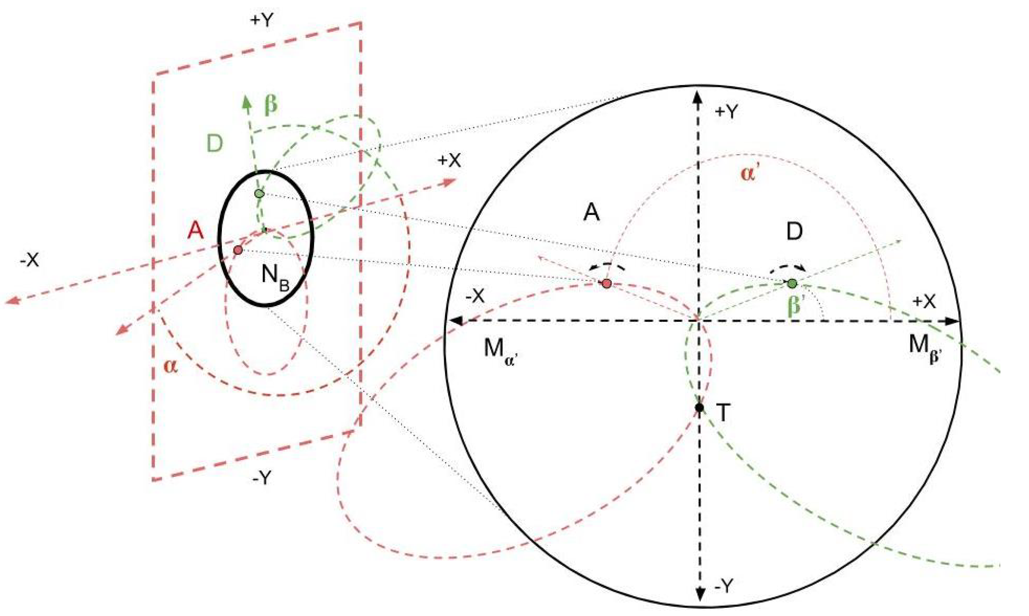
In an unbalanced position, the rate of change of and need not be proportional. However, if the entire figure is rotated into the conventional balanced configuration for any given , then the rate of change of will be exactly opposite , as illustrated in Figure 9. Let and be the angles formed with the negative y-axis in the balanced configuration. By definition of balance about the y-axis, .
This means the intersection point of the two projected ellipses (which may be very close to the z-axis), will always be reached at exactly time (): . This intersection point in the balanced configuration is straight down; it is the point at which the projections are in the same plane (the plane of the z-axis), and at this point, the segmented helix is a toroid-like figure. Since there is always such an intersection point and can be moved through a full rotation, such a toroidal point can always be reached. If the face normals are precisely anti-parallel, this point will occur at the origin, and in that case will be a straight line, which is in a sense a degenerate torus-like figure.
Similarly, the objects can always be twisted to a point where A and D are pointing opposite each other as measured from the origin of the projection plane, so that . This is always the “flat” or maximally extended point of maximum tightness. In the balanced convention, this occurs when the projection points are coincident with the x-axis in the projection plane, as shown in Figure 9. Because in this case the A and D points are always (even in the first case of this proof) at equal angles to the z-axis aligned object axis , the A and D projection points move at the same speed (with respect to ), and they meet the x-axis at the same value.
Thus, when the absolute value of the face normals formed with the z-axis are equal, the objects can be smoothly twisted through a spectrum between the toroid-like figure (zero travel, or , and therefore minimum tightness), and the position of maximal travel. □
It would be more useful and elegant to have a formula for the twist that produces a torus as a function of the joint face normals, which is future work. Nonetheless, in the calculator page the that produces the minimum tightness (torus-like) and maximum tightness (zig-zag) to the nearest 360-degree is numerically calculated, with the labels Minimum Tightness τ and Maximum Tightness τ.
3. Discussion
3.1. Checks and Explorations
3.1.1. Qualitative Observations
When the joint face normals are coplanar vectors, then the minimum tightness is always 0, and the maximum tightness occurs when . These values deviate from 0 and roughly in proportion to the non-coplanarity of the normals.
Varying smoothly varies the tightness of the coiling of the helix, moving through very linear cases towards a torus, to a torus, to a very linear case on the other side.
In fact it is possible that there is always a “tightest coil” which does not self-intersect. If we had many objects, they could be packed into a convenient space by computing the of the tightest non-self-intersecting coil and stacking them this way. If can be changed, perhaps via motors in a robot arm, the object stack smoothly telescopes and contracts forming a linear actuator. A repeated molecular subunit that changed shape in response to an external magnetic or electric field or chemicals in the surrounding environment would be a telescoping nanomachine or nanoactuator.
3.1.2. A Brute-Force Approach to Finding Helix Angle from Twist
The calculation methods described in this paper hardly warrant the name “algorithm” when considered from the view of computational complexity; they are all constant times (for a given fixed precision). Although involving trigonometric functions, they demand no iteration.
This makes it practical to solve some problems by brute-force iteration. An example already calculated is the twist which makes an object product a toroid-like segmented helix, or on the other hand the value that maximizes linear extent and tightness. Future work may allow analytic formulae for as a function of tightness to be developed; in the meantime it is easy enough to simply evaluate objects at many different values to find a desired helix angle , such as 0. Standard numerical optimization can of course be brought to bear, because an objective function that depends on the parameters of the segmented helix can be efficiently computed in constant time.
3.2. Implications
One of the implications of having an easily-calculable understanding of the math is that it may be possible to design helices of any radius and pitch by designing periodic (possibly irregular) objects. Combined with slight irregularities, this means there exists a basis to design molecular helices out of “atoms” which correspond to our objects.
This means that if a structural engineer that wanted to construct a structure exactly 10 m high out of a number of repeated objects cast from concrete with an axis length of exactly m, they would be able to design the conjoining rule easily.
A modular robot constructed out of repetitions of the same shape-changing module will always produce a helix whose precise shape can be controlled by uniformly changing the shape of all of the modules.
3.3. Applying to the Boerdijk–Coxeter Tetrahelix
The Boerdijk–Coxeter tetrahelix (BC helix) (see Figure 10) is a periodic chain of conjoined regular tetrahedra which has been much studied [11,12,13,14] and happens to have irrational measures, making it an ideal test case for these algorithms. Because the face-normals can be calculated and the positions of the elements of the BC helix directly calculated, we can use it to test the algorithms, and in fact these algorithms give the same rotation.
However, it should be cautioned that the helix which Coxeter identified [11] goes through every node of every tetrahedron. Constructing the helix going through only “rail” nodes allows irregular tetrahelices to be designed [14] (see Figure 11). However, the segmented helices defined in this paper do neither; rather, it is most natural to imagine them moving through the centroid of a face of a tetrahedron. This is a segmented helix of very small radius () compared to the other two approaches () which measure the radius to the vertex of the tetrahedron, but it has the advantage that it is far more general. For example, it is clearly defined if one used truncated tetrahedra. The rotation of a segment matches the BC helix analytical solution () (see first line of Table 1), because a screw transformation does not depend on selecting a point for the radius.
In light of Observation 1 and the segmented helix algorithms, it is possible to consider the BC Helix and a variety of other segmented helices generated by face-to-face stacking of Platonic solids, examples called Platonic segmented helices.
Note this also makes clear that in these cases it is necessary to also specify the twist, even if perfect face-to-face matching is required. Thinking of it this way, there are actually three tetrahedral segmented helices, depending on which twist modulo 120° is chosen (keeping the faces matching): the clockwise BC Helix, the anti-clockwise BC Helix, and the not-quite-closed tetrahedral torus, similar in appearance to but not quite the same as toroidal polyhedral [27]. (Five tetrahedra famously lack degrees of being a perfect toroidal polyhedron as can be seen from the website which computes for this case, so the gap is ).
In the case of the icosahedron, there are in fact many possibilities, as one need not choose the precisely opposite face as the joining face, and up to three twists may be chosen.
3.4. Confirming Periodic Twists
The Boerdijk–Coxeter tetrahelix has an irrational rotation about the angle, meaning that is aperiodic. There is no number of perfectly regular tetrahedra that can be joined to get back to exactly the same position. A recent paper by Sadler, Fang, Clawson and Irwin [12] has explored this and given an explicit formula for a twist exactly as defined in this paper in order to produce a periodic tetrahelix.
Their formula for period p is:
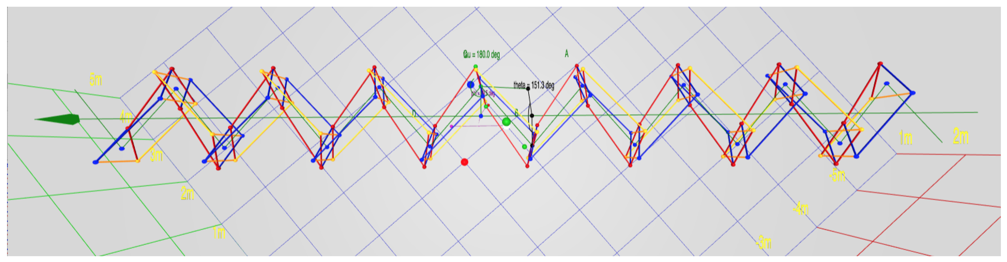
where would be the twist and , the dihedral half-angle of the regular tetrahedron, and m is chosen to satisfy . Seeking a period of 7, we choose to satisfy this condition, and obtain . It is gratifying that this angle does in fact produce a period-7 tetrahelix as shown in Figure 12.
Such a tetrahelix will of course differ to some extent by being more or less “jagged” compared to the BC helix. This related paper [12] has produced an analytic formula specifically related to the tetrahedron. Presumably, the interactive software described here would assist in the search for analytic descriptions of other Platonic helices, or would allow an approximation to be discovered quickly and simply visually.
3.5. The Platonic Helices
In order to demonstrate the utility of the calculations explained in this paper, periodic chains of the five regular Platonic solids joined face-to-face so that their vertices coincide, which form Platonic helices, are explored. Such tetrahelices, icosahelices, octahelices and dodecahelices have been mentioned in a number of papers [28,29,30,31], but not exhaustively studied in the purely helical form. We propose the name cubahelix for the helix made from cubes, as opposed to the equivalent but cumbersome hexahedronahelix. Because in some cases Platonic segmented helices may be found in nature or related to structures found in nature [15,32], it would be convenient to have a table, and images, of all such Platonic segmented helices for reference.
To construct a specific periodic chain from a Platonic solid, one must decide which faces are joined by the rule. Additionally, one must determine a twist as part of the rule, and this twist must be chosen from a small set if the vertices are to coincide. The set of vertex-matching twists differs slightly depending on the face chosen for octahedron, dodecahedron, and icosahedron (but not for the tetrahedron and the cube). The number of twists in a set will always be equal to the number of sides on a face.
Therefore the number of Platonic helices is in principle a summation of a number of faces times a number of sides, or . However, many of the possible helices will be indistinguishable if only the shapes produced are considered, as opposed to considering completely labeled or colored faces. Furthermore, every non-toroidal helix will come in a clockwise and anti-clockwise version. However, it is sensible to disallow rules such as “attach face zero to face zero” which would constitute “doubling back” [28,29]. The transformation matrix for such a rule would be the identity matrix. It produces an object axis of zero length, a radius of zero, and travel of zero. It produces perfect self-intersection—the entire degenerate helix would appear to be simply a single Platonic solid.
Using the math in this paper and a computer, it is easy to evaluate all 180 helices, place them in a table (see Table 1), and group them by radius and travel (collapsing chirality). The result is 28 unique shapes. In this number, no provision was made to exclude self-intersection, which does occur, but might not matter to an aerospace engineer building a collapsible space frame of rods and joints. In the language of Elgersma and Wagon [28,29], not all of the 28 Platonic helices are embedded.
With those caveats, the helices in Table 1, exemplified by accompanying figures and renderable interactively on the calculator page, represent an exhaustive catalog, colloquially called a “zoo”, of all Platonic helices.
In Table 1, column C-Face, refers to the face as numbered by the THREE.js software [26], which is somewhat arbitrary. The # Analogs column gives the number of Platonic helices with the same shape, or the enantiomer of it, that is, the same shape in either the clockwise or anti-clockwise direction. This list can be expanded completely on our interactive website.
Clearly, for each solid there is a change in the twist that keeps the vertices on two joined faces coincidentally and aligned if they start aligned. This is , where n is the number of sides in a face. The base twist that creates a perfect face-to-face match depends not only on the solid but the face it is conjoined to. For each of the Platonic solids, the base angle was found by visual inspection and trial and error. The twist of a species of helix is given in the column below.
Qualitative Descriptions and Interesting Shapes
For fun and to facilitate conversation, we have given all 28 of these Platonic helices descriptive nicknames. A few of these are interesting enough to be worthy of particular mention, and comparing them shows the possibility of designing structures using nothing but Platonic solids. The math in this paper works equally well with irregular shapes as well, allowing continuous spectra of designed structures from repeated shapes or molecules.
- The “Blockhelix” (Figure 13) is a cubic rectilinear structure in which all angles are right angles; nonetheless a segmented helix hides inside it which is perhaps not apparent to the human eye at first glance.
- The “Pearlshaft” (Figure 14). Conjoining parallel faces always produces a shaft. This icosahedron, being relatively round, resembles a string of pearls.
- However, shaft-like helices exist which do not join opposite faces. The “Dodecashaft” (Figure 15) is a remarkably tight non-self-intersecting dodecahelix with very narrow gaps between objects. Such a configuration might be formed by nanofibers under pressure.
- The “Dodecadoubler” (Figure 16) presents the appearance of being a double helix, even though in fact it is a single helix with a simple twist of 72 from the “Dodecashaft”.
- The “Dodecacorkscrew” (Figure 17) is a contrasting example of a loose helix, reminiscent of a corkscrew for opening wine bottles.
- The “Quasi-planar” (Figure 18) icosahelix presents a slowly twisting metahelix, so perhaps 10 icosahedron could be said to “lay flat”. If this were a molecule or a physical structure made of less-than-perfectly rigid members, it might be possible to force it into a pure planar configuration, thus wrapping a cylinder or a plane, studding it with icosahedra.
- “Two Strands” (Figure 19) is similar to the “Dodecadoubler” but even more visually striking. It is reminiscent of a depiction of a DNA double helix.
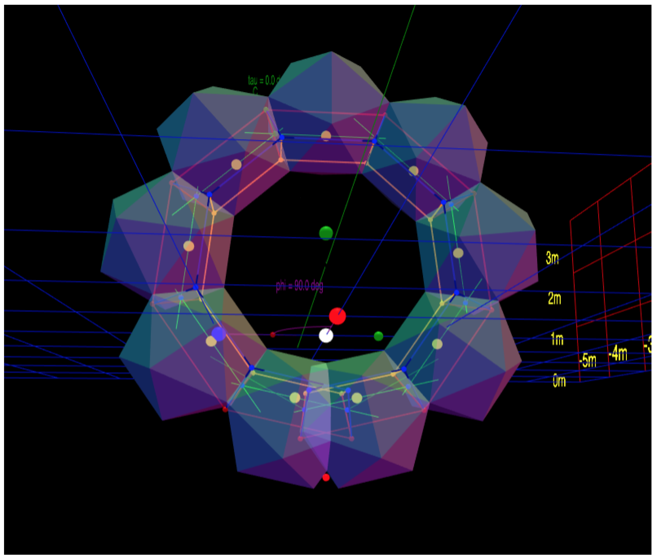
- The “Wheel” (Figure 20) resembles a modern car tire in proportions. All Platonic solids and indeed all shapes have torus-like configurations. In general, they do not “close” perfectly. There is a gap that prevents the final faces from fitting together perfectly. However, a tiny adjustment could be made to the repeated shape to close this gap.
3.6. Future Work
The algorithms and software described herein allow numerical calculation of the intrinsic properties of these Platonic helices, but it would be even better to describe them with closed-form expressions, as Coxeter did for the Boerdijk–Coxeter tetrahelix. The math and the algorithms are simple enough that if coded in a symbolic algebra system, or with careful work, closed-form expressions could be produced for all the regular Platonic helices. These would be interesting if they happen to be short; there is no reason to believe they will be. The same work could be done for the Archimedean solids. The current work would serve as a useful validation check and intuition-builder for such work.
There may exist a closed-form expression for twist which produces the desired helix angle . The website implements an iterative algorithm to find it, which is practical but less elegant.
Funding
This research received no external funding.
Institutional Review Board Statement
Not applicable.
Informed Consent Statement
Not applicable.
Data Availability Statement
Not applicable.
Acknowledgments
Thanks to Eric Lord for their direct communication. The enthusiasm of the participants of the 2018 Public Invention Mathathon initiated this work.
Conflicts of Interest
The author declares no conflict of interest.
References
- Read, R.L. The Story of a Public, Cooperative Mathathon. 2019. Available online: https://medium.com/hackernoon/the-story-of-a-public-cooperative-mathathon-29ea5f4ff538 (accessed on 12 December 2018).
- Lord, E.A. Helical structures: The geometry of protein helices and nanotubes. Struct. Chem. 2002, 13, 305–314. [Google Scholar] [CrossRef]
- Wittenburg, J. Kinematics: Theory and Applications; Springer: Berlin/Heidelberg, Germany, 2016. [Google Scholar]
- Abbasi, N.M. Review of the Geomety of Screw Axes. 2015. Available online: http://www.12000.org/my_notes/screw_axis/index.htm#x1-190006 (accessed on 26 June 2019).
- Kahn, P.C. Defining the axis of a helix. Comput. Chem. 1989, 13, 185–189. [Google Scholar] [CrossRef]
- Wikipedia Contributors. Screw Axis—Wikipedia, The Free Encyclopedia. 2019. Available online: https://en.wikipedia.org/w/index.php?title=Screw_axis&oldid=1092456924 (accessed on 6 June 2019).
- Read, R.L. Segmented Helix JavaScript Code. 2019. Available online: https://github.com/PubInv/segmented-helixes/blob/master/js/segment_helix_math.js (accessed on 26 June 2019).
- Read, R.L. Segmented Helix Interactive 3D Calculator. 2019. Available online: https://pubinv.github.io/segmented-helixes/index.html (accessed on 26 June 2019).
- Enkhbayar, P.; Damdinsuren, S.; Osaki, M.; Matsushima, N. HELFIT: Helix fitting by a total least squares method. Comput. Biol. Chem. 2008, 32, 307–310. [Google Scholar] [CrossRef] [PubMed]
- Lee, H.S.; Choi, J.; Yoon, S. QHELIX: A computational tool for the improved measurement of inter-helical angles in proteins. Protein J. 2007, 26, 556–561. [Google Scholar] [CrossRef] [PubMed]
- Coxeter, H.S.M. The simplicial helix and the equation tan(n θ) = n tan(θ). Canad. Math. Bull. 1985, 28, 385–393. [Google Scholar] [CrossRef]
- Sadler, G.; Fang, F.; Clawson, R.; Irwin, K. Periodic Modification of the Boerdijk–Coxeter Helix (tetrahelix). Mathematics 2019, 7, 1001. [Google Scholar] [CrossRef] [Green Version]
- Fuller, R.; Applewhite, E. Synergetics: Explorations in the Geometry of Thinking; Macmillan: New York, NY, USA, 1982. [Google Scholar]
- Read, R. Transforming Optimal Tetrahelices between the Boerdijk–Coxeter Helix and a Planar-faced Tetrahelix. J. Mech. Robot. 2018, 10, 051001. [Google Scholar] [CrossRef]
- Pearce, P. Structure in Nature Is a Strategy for Design; MIT Press: Cambridge, MA, USA, 1990. [Google Scholar]
- Read, R.L. Calculating the Segmented Helix Formed by Repetitions of Identical Subunits. In Proceedings of the IMA Conference on Mathematics of Robotics, Manchester, UK, 9–11 September 2020; Springer: Berlin/Heidelberg, Germany, 2020; pp. 115–124. [Google Scholar]
- Wikipedia Contributors. Helix—Wikipedia, The Free Encyclopedia. 2019. Available online: https://en.wikipedia.org/w/index.php?title=Helix&oldid=1092456083 (accessed on 21 November 2019).
- Wikipedia Contributors. Helix Angle—Wikipedia, The Free Encyclopedia. 2019. Available online: https://en.wikipedia.org/w/index.php?title=Helix_angle&oldid=1099199034 (accessed on 17 June 2019).
- Gu, L.; Lei, P.; Hong, Q. Research on Discrete Mathematical Model of Special Helical Surface. In Green Communications and Networks; Springer: Dordrecht, The Netherlands, 2012; pp. 793–800. [Google Scholar]
- Wikipedia Contributors. Chasles’ Theorem (Kinematics)—Wikipedia, The Free Encyclopedia. 2018. Available online: https://en.wikipedia.org/w/index.php?title=Chasles%27_theorem_(kinematics)&oldid=1096921886 (accessed on 19 June 2019).
- Wikipedia Contributors. Rigid Transformation—Wikipedia, The Free Encyclopedia. 2019. Available online: https://en.wikipedia.org/w/index.php?title=Rigid_transformation&oldid=1090098850 (accessed on 19 June 2019).
- Wikipedia Contributors. Rotation Matrix—Wikipedia, The Free Encyclopedia. 2019. Available online: https://en.wikipedia.org/w/index.php?title=Rotation_matrix&oldid=1098322456 (accessed on 21 June 2019).
- Funda, J.; Paul, R.P. A computational analysis of screw transformations in robotics. IEEE Trans. Robot. Autom. 1990, 6, 348–356. [Google Scholar] [CrossRef]
- Wikipedia Contributors. Helical Wheel—Wikipedia, the Free Encyclopedia. 2018. Available online: https://en.wikipedia.org/w/index.php?title=Helical_wheel&oldid=1060513105 (accessed on 13 July 2019).
- Wolfram Research, Inc. Mathematica, Version 12.0; Wolfram Research, Inc.: Champaign, IL, USA, 2019.
- Dirksen, J. Learning Three.js: The JavaScript 3D Library for WebGL; Packt Publishing Ltd.: Birmingham, UK, 2013. [Google Scholar]
- Wikipedia Contributors. Toroidal Polyhedron—Wikipedia, the Free Encyclopedia. 2018. Available online: https://en.wikipedia.org/w/index.php?title=Toroidal_polyhedron&oldid=1090623046 (accessed on 13 July 2019).
- Elgersma, M.; Wagon, S. The Quadrahelix: A Nearly Perfect Loop of Tetrahedra. arXiv 2016, arXiv:1610.00280. [Google Scholar]
- Elgersma, M.; Wagon, S. An asymptotically closed loop of tetrahedra. Math. Intell. 2017, 39, 40–45. [Google Scholar] [CrossRef]
- Babiker, H.; Janeczko, S. Combinatorial Representation of Tetrahedral Chains. Commun. Inf. Syst. 2015, 3, 331–359. [Google Scholar] [CrossRef]
- Lord, E.; Ranganathan, S. Sphere packing, helices and the polytope {3, 3, 5}. Eur. Phys. J. D At. Mol. Opt. Plasma Phys. 2001, 15, 335–343. [Google Scholar] [CrossRef] [Green Version]
- Lord, E.; Ranganathan, S. The γ-brass structure and the Boerdijk–Coxeter helix. J. Non-Cryst. Solids 2004, 334, 121–125. [Google Scholar] [CrossRef]
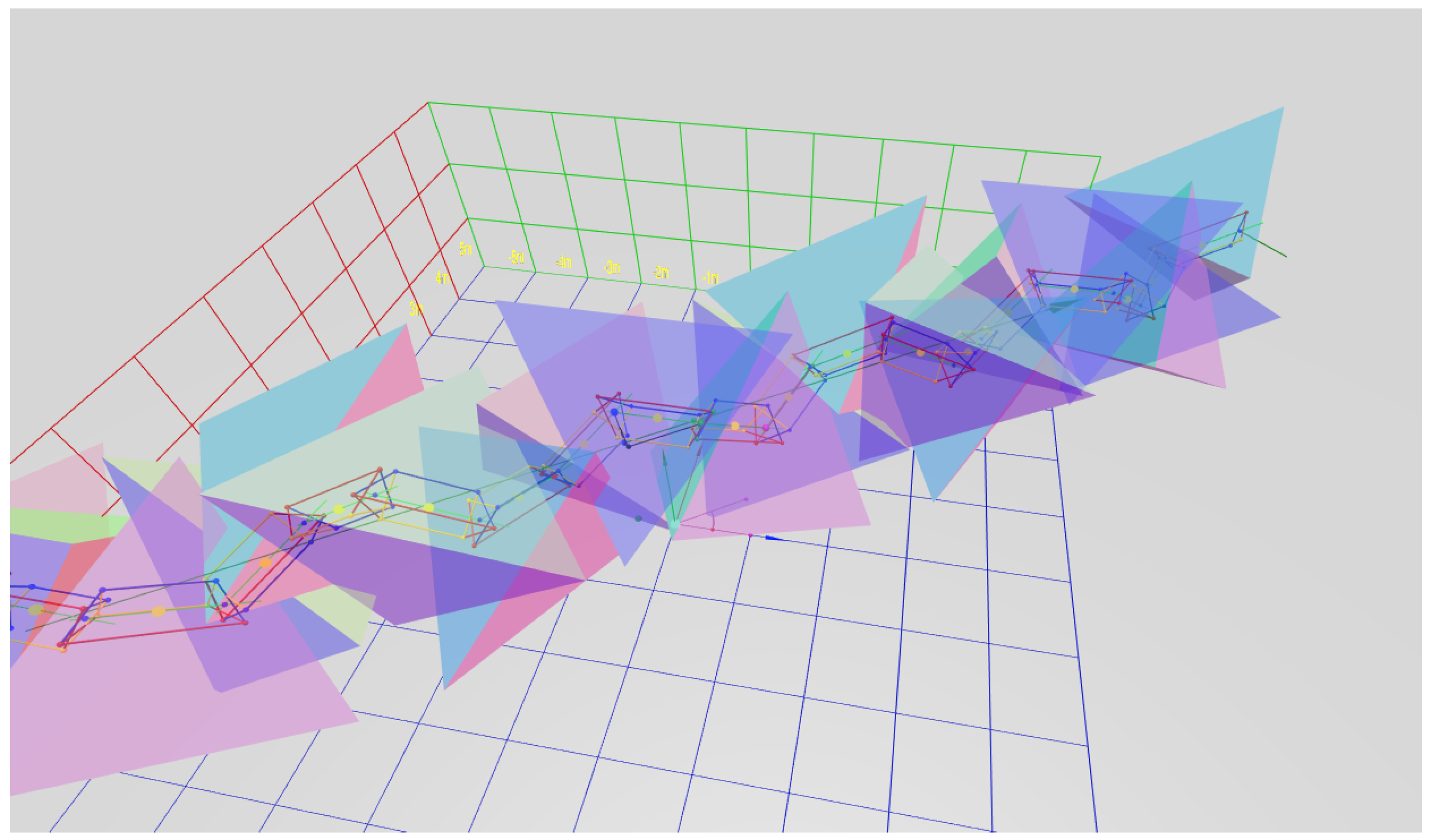
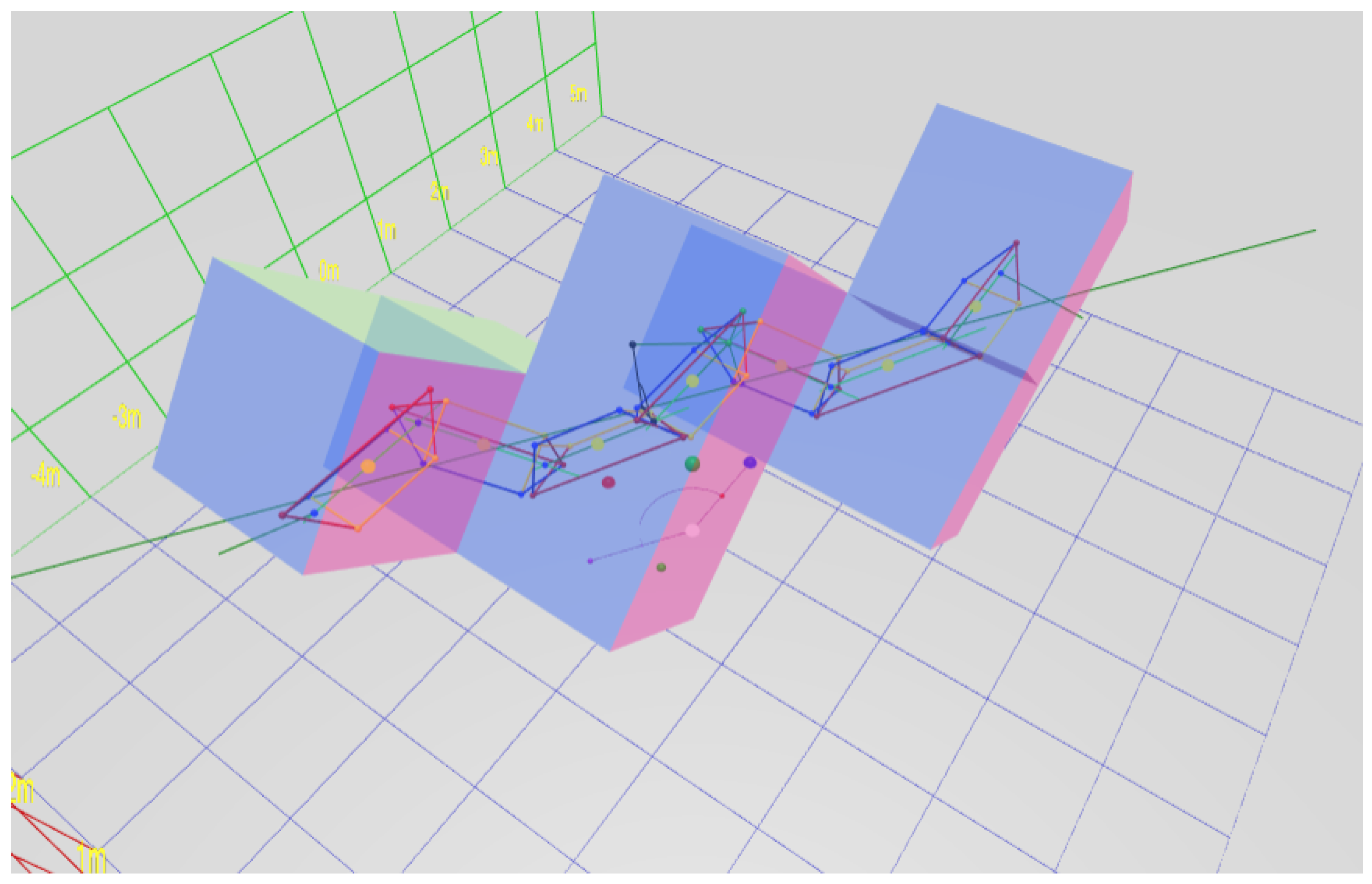
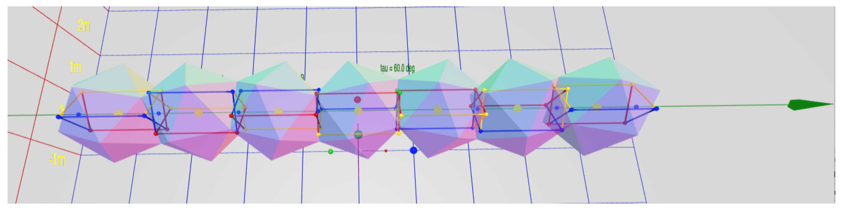
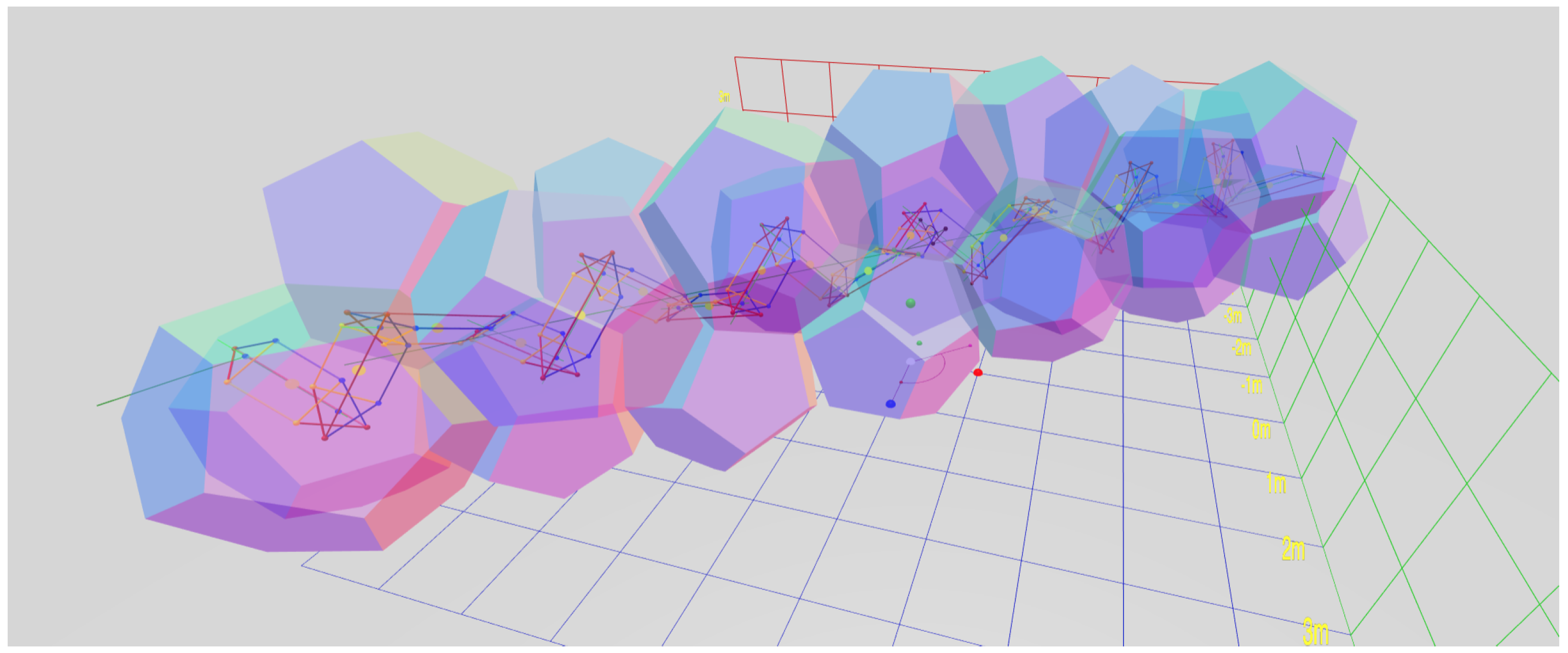
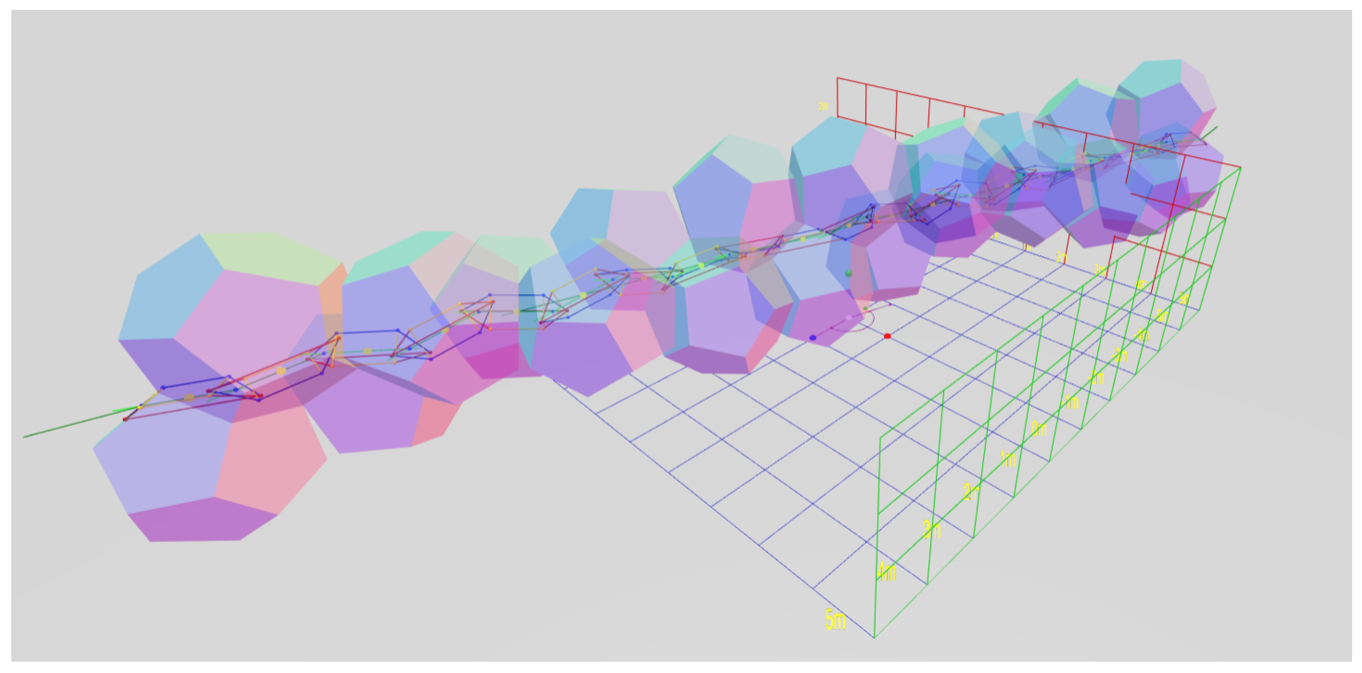
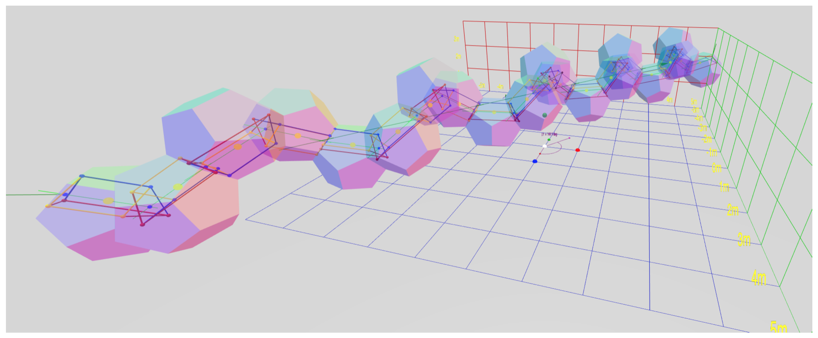
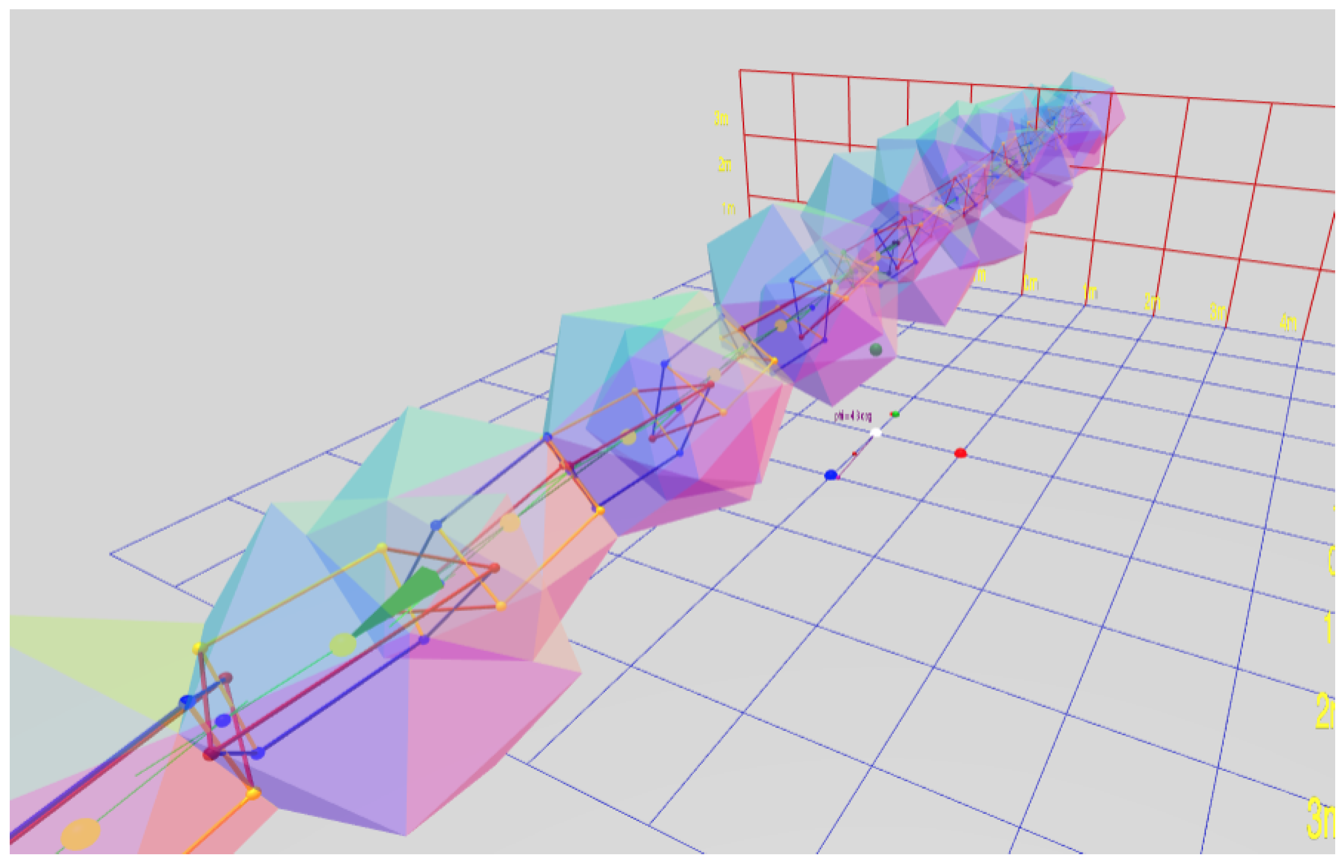
Figure 1.
Example Segmented Helix Generated From the Dodecahedron.

Figure 2.
A 2D analog of a helix generated by repeated subunits.

Figure 3.
Naming of measures.

Figure 4.
A Planar Zig-Zag.

Figure 5.
Three Symmetric Members.

Figure 6.
A Balanced Configuration.

Figure 7.
Twist Spectrum Proof Diagram.

Figure 8.
Equal face angle magnitudes.

Figure 9.
Balanced Projection.

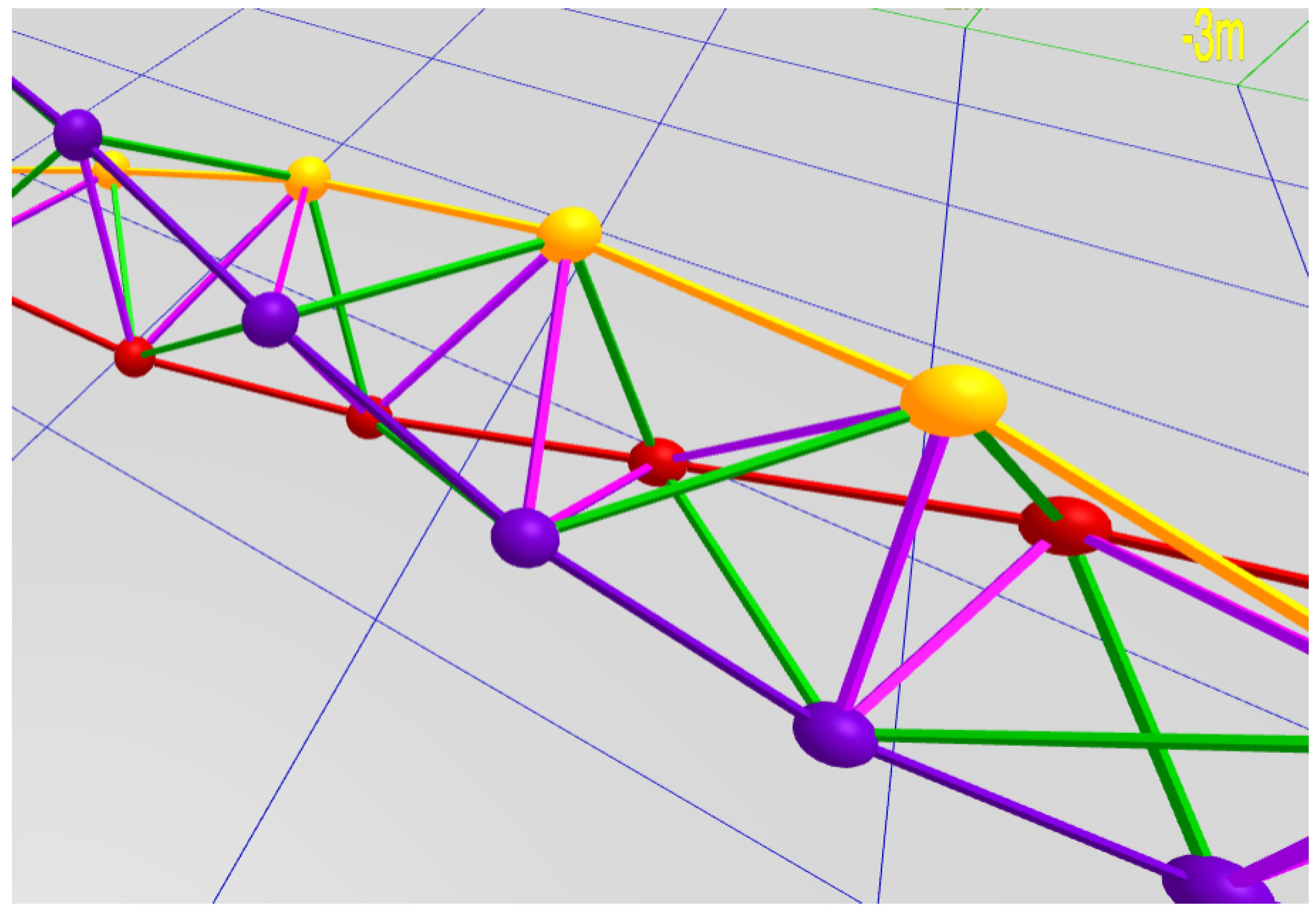
Figure 10.
Boerdijk–Coxeter Tetrahelix.

Figure 11.
Node (Coxeter) helix (in black) and rail helices (in red, blue, and yellow), different than joint helices.
Figure 11.
Node (Coxeter) helix (in black) and rail helices (in red, blue, and yellow), different than joint helices.

Figure 12.
A Period-7 Tetrahelix generated with a twist of 80.43°.

Figure 13.
The Blockhelix.

Figure 14.
The Pearlshaft.

Figure 15.
The Dodecashaft.

Figure 16.
The Dodecadoubler.

Figure 17.
The Dodecacorkscrew.

Figure 18.
Quasi-planar icosahelix.

Figure 19.
Two Strands.

Figure 20.
The Wheel.


Table 1.
The Platonic helices.
| Name | Solid | # of Analogs | C-Face # | Radius | d | |||
|---|---|---|---|---|---|---|---|---|
| Tetrahelix | Tet | 6 | 1 | −120 | 0.094 | 131.810 | −0.516 | 161.565 |
| Tetratorus | Tet | 3 | 1 | 0 | 0.471 | 70.529 | 0.000 | 90.000 |
| Boxbeam | Cub | 4 | 1 | −180 | 0.000 | 0.000 | 1.000 | 0.000 |
| Staircase | Cub | 4 | 2 | −180 | 0.000 | 0.000 | 0.707 | 0.000 |
| Blockhelix | Cub | 8 | 2 | −90 | 0.236 | 120.000 | −0.577 | 144.736 |
| Cubatorus | Cub | 4 | 2 | 0 | 0.500 | 90.000 | 0.000 | 90.000 |
| Octabeam | Oct | 3 | 5 | −60 | 0.000 | 0.000 | 1.155 | 0.000 |
| Octaspiky | Oct | 6 | 1 | −120 | 0.148 | 146.443 | −0.603 | 154.761 |
| Octamedium | Oct | 6 | 2 | −120 | 0.163 | 131.810 | −0.894 | 161.565 |
| Octagear | Oct | 3 | 1 | 0 | 0.408 | 109.471 | 0.000 | 90.000 |
| Treestar | Oct | 3 | 2 | 0 | 0.816 | 70.529 | 0.000 | 90.000 |
| Dodecabeam | Dod | 5 | 8 | −108 | 0.000 | 0.000 | 1.589 | 0.000 |
| Dodecadoubler | Dod | 10 | 1 | −144 | 0.113 | 161.301 | −0.805 | 164.550 |
| The Alternater | Dod | 10 | 2 | −144 | 0.118 | 149.520 | −1.333 | 170.306 |
| Dodecashaft | Dod | 10 | 1 | −72 | 0.351 | 129.657 | −0.543 | 130.501 |
| Dodecagear | Dod | 5 | 1 | 0 | 0.491 | 116.565 | 0.000 | 90.000 |
| Dodecacorkscrew | Dod | 10 | 2 | −72 | 0.546 | 93.026 | −1.095 | 144.110 |
| Dodecadonut | Dod | 5 | 2 | 0 | 1.286 | 63.435 | 0.000 | 90.000 |
| Pearlshaft | Ico | 3 | 13 | −60 | 0.000 | 0.000 | 1.589 | 0.000 |
| Quasi−planar | Ico | 6 | 8 | 165 | 0.049 | 167.764 | 1.294 | 4.347 |
| Two Strands | Ico | 6 | 1 | 120 | 0.137 | 159.446 | 0.499 | 28.340 |
| Slow Twist | Ico | 6 | 12 | 120 | 0.169 | 124.309 | 1.454 | 11.641 |
| Rock Candy | Ico | 12 | 2 | 120 | 0.204 | 146.443 | 0.830 | 25.239 |
| Icosa Tree Star | Ico | 3 | 1 | 0 | 0.304 | 138.190 | 0.000 | 90.000 |
| Icosacorkscrew | Ico | 6 | 8 | −75 | 0.512 | 99.253 | −1.037 | 143.042 |
| Planar point cluster | Ico | 6 | 2 | 0 | 0.562 | 109.471 | 0.000 | 90.000 |
| Big Icosacorkscrew | Ico | 6 | 8 | 45 | 0.803 | 82.064 | 0.756 | 54.343 |
| The Wheel | Ico | 3 | 12 | 0 | 2.080 | 41.810 | 0.000 | 90.000 |
Publisher’s Note: MDPI stays neutral with regard to jurisdictional claims in published maps and institutional affiliations. |
© 2022 by the author. Licensee MDPI, Basel, Switzerland. This article is an open access article distributed under the terms and conditions of the Creative Commons Attribution (CC BY) license (https://creativecommons.org/licenses/by/4.0/).
Share and Cite
MDPI and ACS Style
Read, R.L. Calculating the Segmented Helix Formed by Repetitions of Identical Subunits thereby Generating a Zoo of Platonic Helices. Mathematics 2022, 10, 2533. https://0-doi-org.brum.beds.ac.uk/10.3390/math10142533
AMA Style
Read RL. Calculating the Segmented Helix Formed by Repetitions of Identical Subunits thereby Generating a Zoo of Platonic Helices. Mathematics. 2022; 10(14):2533. https://0-doi-org.brum.beds.ac.uk/10.3390/math10142533
Chicago/Turabian StyleRead, Robert L. 2022. "Calculating the Segmented Helix Formed by Repetitions of Identical Subunits thereby Generating a Zoo of Platonic Helices" Mathematics 10, no. 14: 2533. https://0-doi-org.brum.beds.ac.uk/10.3390/math10142533
Note that from the first issue of 2016, this journal uses article numbers instead of page numbers. See further details here.