Using Value-Based Potentials for Making Approximate Inference on Probabilistic Graphical Models

Abstract

The computerization of many everyday tasks generates vast amounts of data, and this has lead to the development of machine-learning methods which are capable of extracting useful information from the data so that the data can be used in future decision-making processes. For a long time now, a number of fields, such as medicine (and all healthcare-related areas) and education, have been particularly interested in obtaining relevant information from this stored data. This interest has resulted in the need to deal with increasingly complex problems which involve many different variables with a high degree of interdependency. This produces models (and in our case probabilistic graphical models) that are difficult to handle and that require very efficient techniques to store and use the information that quantifies the relationships between the problem variables. It has therefore been necessary to develop efficient structures, such as probability trees or value-based potentials, to represent the information. Even so, there are problems that must be treated using approximation since this is the only way that results can be obtained, despite the corresponding loss of information. The aim of this article is to show how the approximation can be performed with value-based potentials. Our experimental work is based on checking the behavior of this approximation technique on several Bayesian networks related to medical problems, and our experiments show that in some cases there are notable savings in memory space with limited information loss.

1. Introduction

Probabilistic Graphical Models (PGMs) [1,2,3] are a powerful framework to encode problems under uncertainty. PGMs are able to combine graphs and probability theory to compactly represent the probabilistic dependency between random variables. Any PGM can be defined by its two components:

• Qualitative component, given by a directed, acyclic graph (DAG), where each node represents a random variable, and the presence of an edge connecting two of these implies mutual dependency.
• Quantitative component, given by a set of parameters that quantify the degree of dependence between the variables.

One of the most interesting properties of PGMs over discrete domains such as Bayesian networks (BNs) [4,5] and influence diagrams (IDs) [6,7] is the efficient representation of joint probability distributions, and traditionally marginal or conditional probability distributions and utility functions are represented with tables or unidimensional arrays (1DA in general). However, as the size of 1DAs grows exponentially with the number of variables, an exact representation might be arduous or even impossible (due to memory space restrictions). Even in cases where problem representation using 1DA is possible, it may be difficult to perform subsequent inference tasks as new potentials may appear larger than the initial ones.

This difficulty originates some works focused on improving the way of performing operations with probability distribution and utility functions as a way to alleviate the computational cost in complex models [8]. And another approaches have been explored over the years in the search for efficient alternative representations to 1DAs, which are able to work with complex models. Successful examples are standard and binary probability trees (PTs and BPTs) [9,10,11,12,13]. Despite the advantages that these offer compared to the use of 1DA, they also present certain limitations, and not all context-specific independences can result in smaller representations and therefore in memory space savings.

Another very well-studied strategy for saving memory space is to approximate the structures, such as in PTs, by accepting a loss of information [14,15]. This operation is called pruning and the PTs which have been pruned are called pruned probability trees (PPTs). This operation consists of replacing certain contiguous values with their average value, always remembering to select those values that produce the smallest information loss.

Value-based potentials (VBPs) [16] were recently introduced. These structures take advantage of the repetition of values, regardless of the order in which they appear. VBPs were tested with several BNs included in the bnlearn repository [17,18] and the UAI inference competitions [19,20]. The paper compares the memory spaces required for representing potentials with 1DAs, PTs, PPTs, and VBPs. The comparison demonstrates that there is an overall reduction in memory space when VBPs are used. Their use is justified by observing that, in a large number of BNs representing real-world problems (in the medical field, for example), many repeated values appear in the potentials which quantify the probabilistic relationships. For example, all those impossible events will have been assigned a probability value equal to 0. Another source of repetition can occur in situations in which the models include subjectively assigned probabilities through interviews with experts. Normally, the assigned probabilities are reduced to a very limited set of values (for example, 0.25, 0.4, etc., and it is difficult for an expert to indicate that the probability of an event occurring is 0.23678).

Taking into account all of the previously mentioned work, the aim of our study will be to make VBPs even more compact and to define an algorithm to approximate them. Such an algorithm will be an iterative process, and each step will keep the approximated VBP with the minimum Kullback–Leibler divergence in relation to the original one, thereby minimizing loss of information.

This paper is organized as follows: Section 2 defines some necessary basic concepts and notation; Section 3 contains the theory about classical structures and alternative VBPs; Section 4 introduces the prerequisites for the approximation of VBPs and the approximation algorithm itself; Section 5 studies the empirical evaluation of the algorithm by applying it to real BNs; and finally Section 6 outlines our conclusions and presents our future lines of research.

2. Basic Definitions and Notation

Let $\mathbf{X}=\{X_1,X_2,\dots ,X_N\}$ be a finite set of discrete random variables. For the sake of simplicity, the states of each variable $X_i$ (its domain) are assumed to be integers and represented as ${\mathsf{\Omega }}_{X_i}$. The values for $X_i$ are noted in lowercase ${\mathsf{\Omega }}_{X_i}=\{x_{i,j}:j=1,2,\dots ,k_i\}$. $|{\mathsf{\Omega }}_{X_i}|$ denotes the cardinality of the variable, i.e., the number of elements in its domain ($|{\mathsf{\Omega }}_{X_i}|=k_i$).

The Cartesian product ${\prod }_{X_i\in \mathbf{X}}{\mathsf{\Omega }}_{X_i}$ will be denoted as ${\mathsf{\Omega }}_{\mathbf{X}}$ and its elements, called configurations of $\mathbf{X}$, are defined by $\mathbf{x}:=\{X_1=x_1,X_2=x_2,\dots ,X_N=x_n\}$, or $\mathbf{x}:=\{x_1,x_2,\dots ,x_n\}$ (if the variables are obvious from the context). A function defined over a subset of variables $\mathbf{Y}\subseteq \mathbf{X}$ and taking values in ${\mathbb{R}}_0^{+}$ will be termed as a potential $\varphi \left(\mathbf{Y}\right)$.

Example 1.

Let us consider the variables $X_1$, $X_2$, and $X_3$, with 2, 3, and 2 possible states, respectively. Then $\varphi (X_1,X_2,X_3)$ is a potential defined on such variables with the values assigned to each configuration shown in Figure 1. This potential expresses the conditional distribution $P\left(X_3\right|X_1,X_2)$.

In order for some of the structures considered in our work to be better understood, we need to clarify the concept of the index of configuration. This is a unique, numeric identifier which represents each configuration on a given domain ${\mathsf{\Omega }}_{\mathbf{X}}$. Let us consider that the indices start at 0 and end on $|{\mathsf{\Omega }}_{\mathbf{X}}|-1$. In the given Example 1, index 0 is associated with the configuration $\{0,0,0\}$, index 1 to $\{0,0,1\}$, and so on until the last one, 11, which is associated with $\{1,2,1\}$ (these indices are shown in the left-most column in Figure 1).

There is a relation between indices and configurations based on the concept of weight (otherwise known as stride or step size). Assuming an order between variables $\mathbf{X}=\{X_1\dots X_N\}$, each variable $X_i\in \mathbf{X}$ has an associated weight $w_i$ that may be computed as follows (variable with index N has the lowest weight):

$$w_i=\left\{\begin{array}{c}\hfill 1ifi=N\hfill \\ \hfill |{\mathsf{\Omega }}_{X_{i+1}}|·w_{i+1}otherwise.\hfill \end{array}\right.$$

(1)

The index corresponding to a certain configuration $\mathbf{x}=\{x_1,x_2,\dots ,x_N\}$ can be computed as:

$$index\left(\mathbf{x}\right)=\prod _{i=1}^N{x}_i·w_i.$$

(2)

Example 2.

Considering the potential described in Example 1, the weights are $w_3=1,w_2=2,w_1=6$, and the indices assigned to configurations are presented below:

$$\begin{array}{c}\hfill index\left(\right\{0,0,0\left\}\right)=0·6+0·2+0·1=0\\ \hfill index\left(\right\{0,0,1\left\}\right)=0·6+0·2+1·1=1\\ \hfill index\left(\right\{0,1,0\left\}\right)=0·6+1·2+0·1=2\\ \hfill .............................\\ \hfill index\left(\right\{1,2,1\left\}\right)=1·6+2·2+1·1=11\end{array}$$

More specifically, the value of a particular variable $X_i$ in a configuration linked to an index k, denoted by ${\mathbf{x}}^{\left(k\right)}$ and satisfying $index\left({\mathbf{x}}^{\left(k\right)}\right)=k$, can be computed as:

$$x_i=(k//w_i)\%\left|{\mathsf{\Omega }}_{X_i}\right|,$$

(3)

where $//$ denotes integer division and % the modulus of the division.

As we mentioned previously, the association between indices and configurations requires that the variable order in the domain be known. Any order is valid, but by default, we will consider the order in which variables are written (e.g., for potential $\varphi (X,Y,Z)$, the first variable would be X). Additionally, we consider that the first variable has the highest weight. However, the opposite approach could also be considered.

The links in the network define a set of conditional dependences and independences that are expressed as $X{\perp }_{\mathbf{Z}}Y$. This expression indicates that X is independent of Y once the values of the variables in $\mathbf{Z}$ are known. The Markov blanket of X, $mb\left(X\right)$, contains its parents $pa\left(X\right)$, its children $ch\left(X\right)$, and the parents of the children $pa\left(ch\right(X\left)\right)$; it is the set of variables that makes X be independent of the other variables $\mathbf{Z}$, $\mathbf{Z}=\mathbf{X}\setminus \{X\cup mb(X\left)\right\}$, once the value of variables in $mb\left(X\right)$ is known, i.e., $X{\perp }_{mb\left(X\right)}\mathbf{Z}$. The in-degree of X is the number of parents $\left|pa\right(X\left)\right|$, and the out-degree is the number of children $\left|ch\right(X\left)\right|$. The average degree considers the values of in-degree and out-degree. These values are used to characterize the BNs used for experiments (see details in Table 5).

3. Representation of Potentials

3.1. Classic Structures

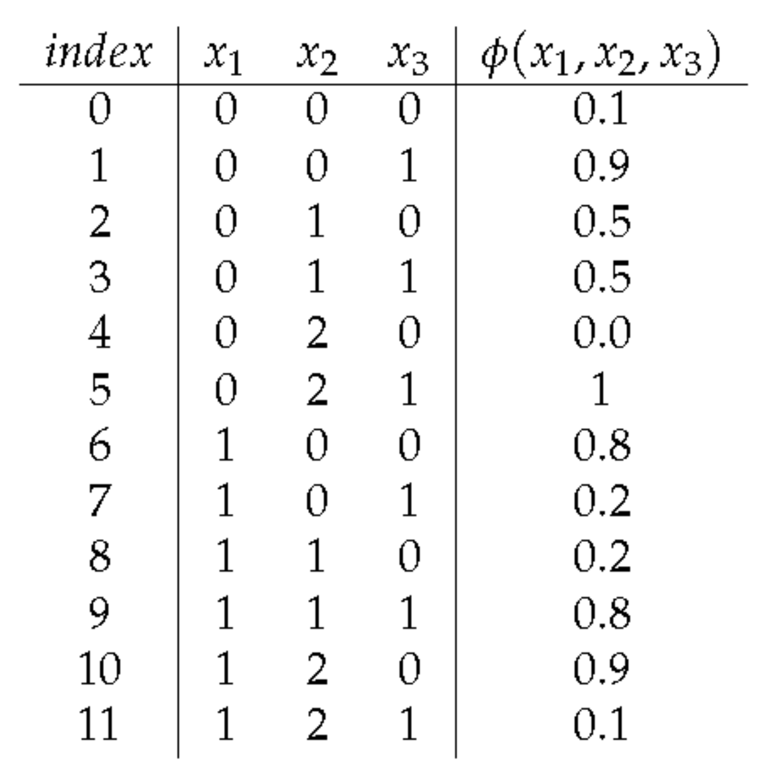
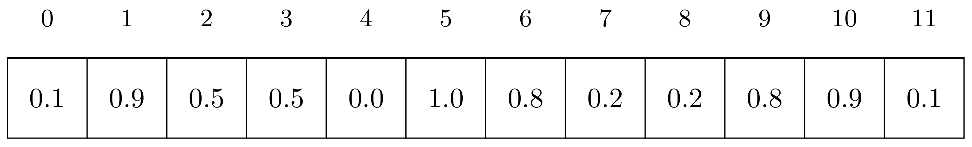
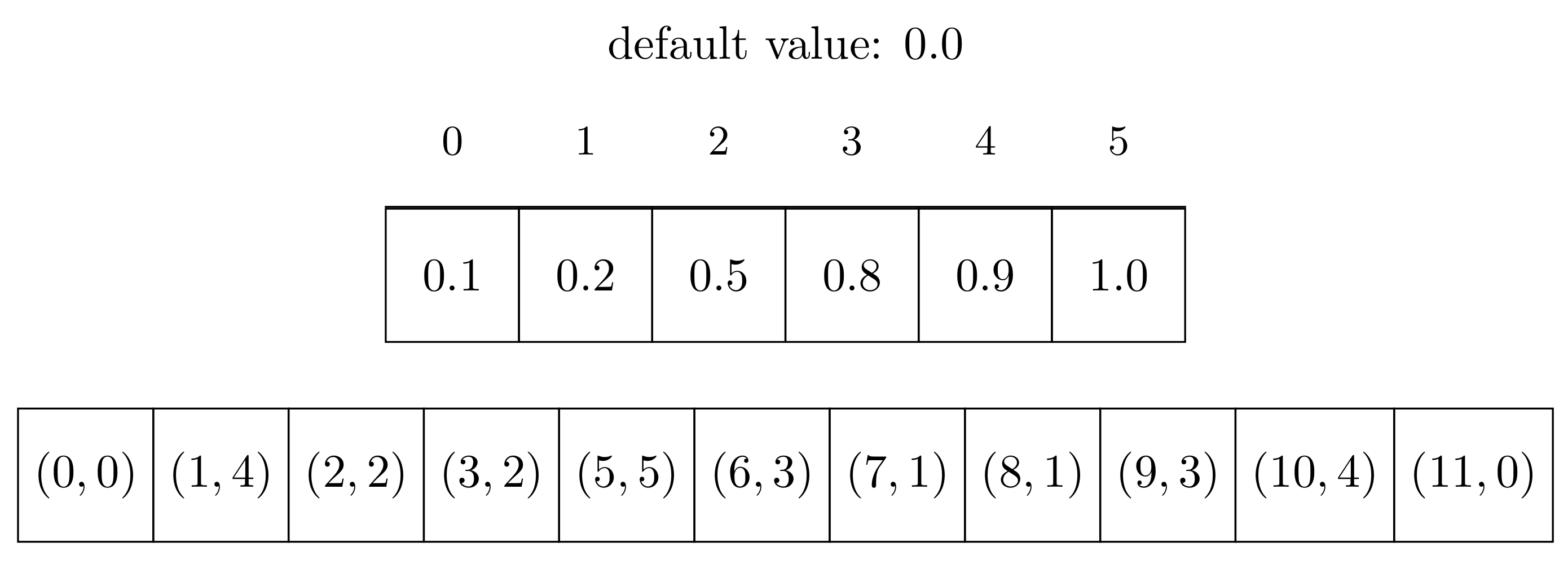
3.1.1. 1D-Arrays

A one-dimensional or single-dimensional array (1DA) is a storage structure for elements of the same nature, which enables every element to be accessed individually by specifying the index corresponding to the position where it is located.

Let $\varphi$ be a potential defined over a set of N variables, $\varphi$ can be represented by an array ${\mathcal{A}}_{\varphi }$ as:

$${\mathcal{A}}_{\varphi }:=\left[\varphi (0,\dots 0),\varphi (0,\dots 1),\dots ,\varphi \left(\right|{\mathsf{\Omega }}_{X_1}|-1,\dots ,|{\mathsf{\Omega }}_{X_N}|-1)\right].$$

(4)

The size of a 1DA, denoted by $size\left({\mathcal{A}}_{\varphi }\right)$, is the number of entries, or the number of configurations of the potential.

Example 3.

The potential $\varphi (X_1,X_2,X_3)$ given in Example 1 can be represented as the following 1DA with 12 entries (see Figure 2).

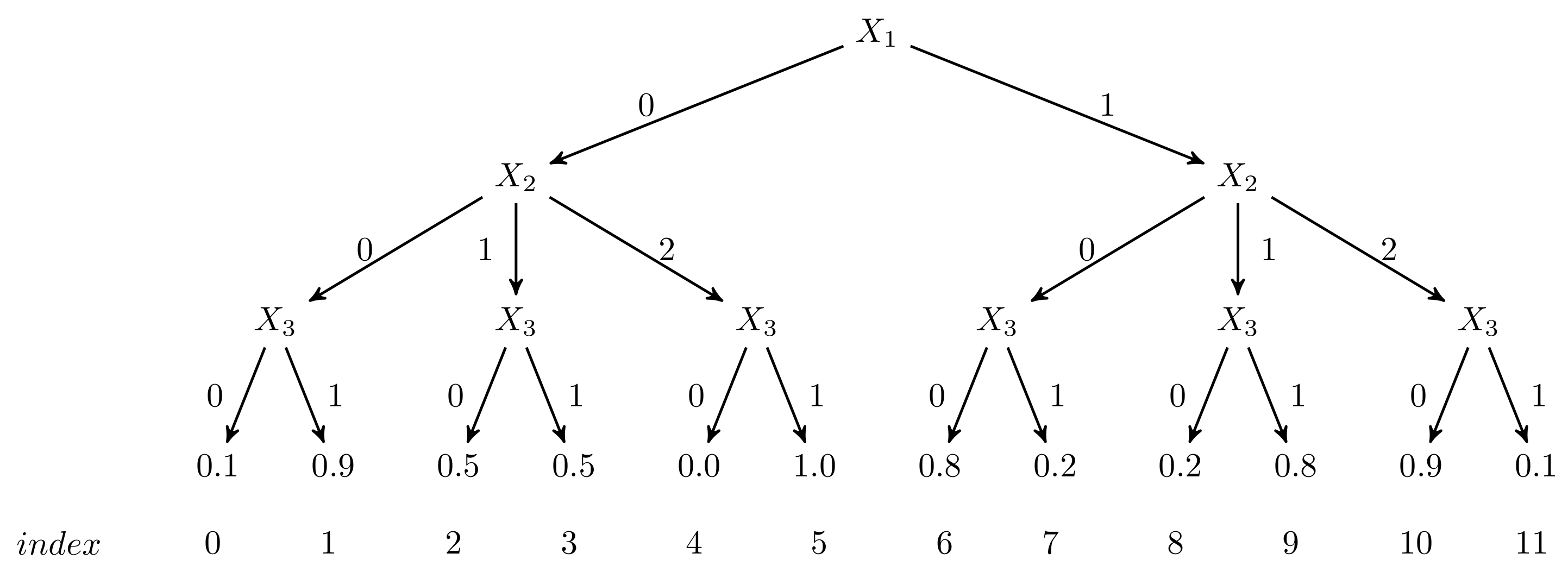
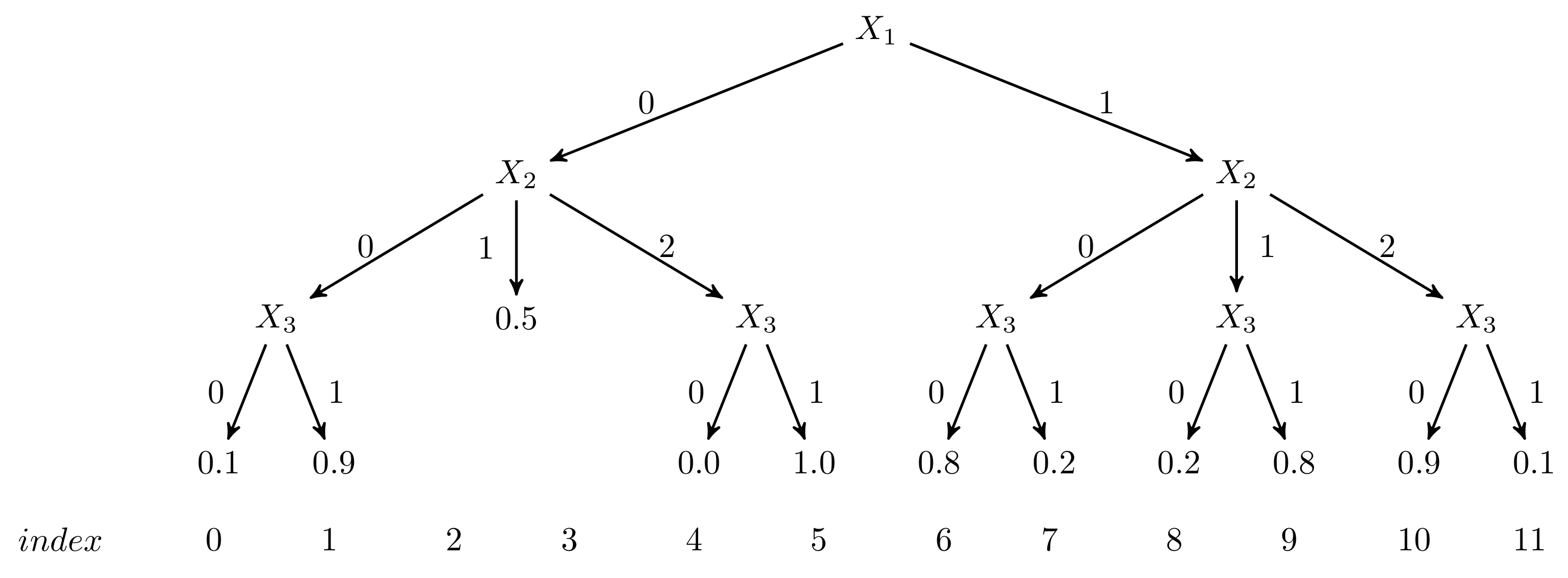
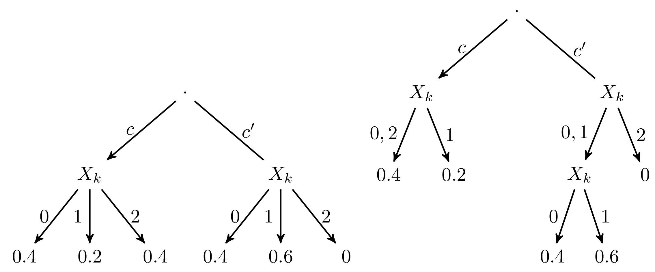
3.1.2. Probability Trees

A probability tree (PT) represents a given potential $\varphi :{\mathsf{\Omega }}_{\mathbf{X}}\to {\mathbb{R}}_0^{+}$, and allows exact or approximate operations over it [11,12,13]. A probability tree $\mathcal{T}$ is a directed and labeled tree, where each internal node represents one variable and each leaf node a non-negative real number. Each internal node will have as many exiting arcs as the number of states that the variable labeling the node has. The size of a PT, $size\left(\mathcal{T}\right)$, is defined as the number of nodes it contains.

Example 4.

The same potential given in the previous example is presented in Figure 3 as a PT. This PT has 21 nodes (12 leaves and 9 internal nodes).

PTs can take advantage of context-specific independences [9] by combing equal values into a single one. This operation is called pruning, and once PTs have been pruned, they are known as pruned probability trees (PPTs).

Example 5.

The potential in the previous examples presents a context-specific independence that enables its size to be reduced: the value for $X_1=0,X_2=1$ is $0.5$, regardless of the value of $X_3$. Once the pruning is complete, the result is a PPT consisting of 19 nodes (11 leaves and 8 internal nodes) and this is shown in Figure 4.

A variant to a PT is the binary probability tree or BPT [10,14,15]. In BPTs, two arcs exit from each internal node, so one variable can label several nodes in a path from root to leaf node. An example of BPT is presented in Figure 5 and described in the following example.

Example 6.

On the left, a given PT is represented, and two equal values ($0.4$) can be observed for c configuration (left sub-tree) but related to two different values of $X_k$. Both values can therefore be combined to produce the BPT on the right-hand side of Figure 5. It is now apparent that the leftmost branch of $X_k$ simultaneously represents values for $X_k=0$ and $X_k=2$.

With this property, although BPTs can avoid more repetitions of values than PPTs, there are still situations in which repetitions cannot be avoided. This is the case for the values $0.4$ of the configurations given by $c^{\prime },x_k=2$ and $c,x_k=0$. Therefore, as we mentioned previously, both PPTs and BPTs introduce the possibility of saving memory space by combining values under pretty specific circumstances, but are not able to make the structure more efficient otherwise. This fact opens various possible avenues of research into how to exploit different patterns. In many cases, some combinations of values are not allowed and are represented by 0’s or some values are repeated several times; a proper efficient structure should be able to somehow compact the information using such patterns.

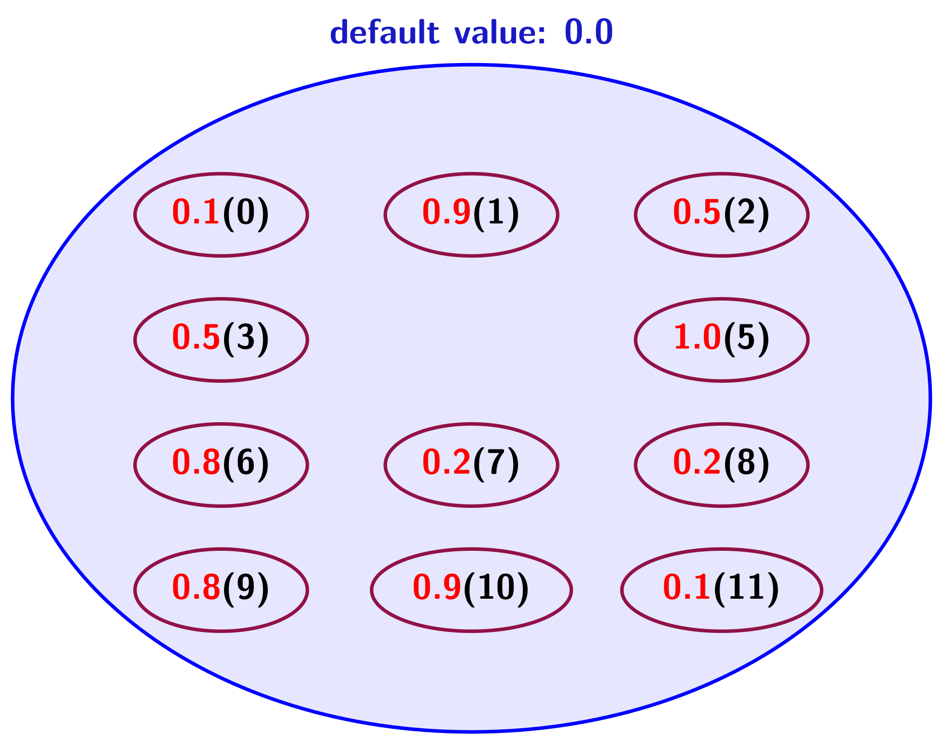
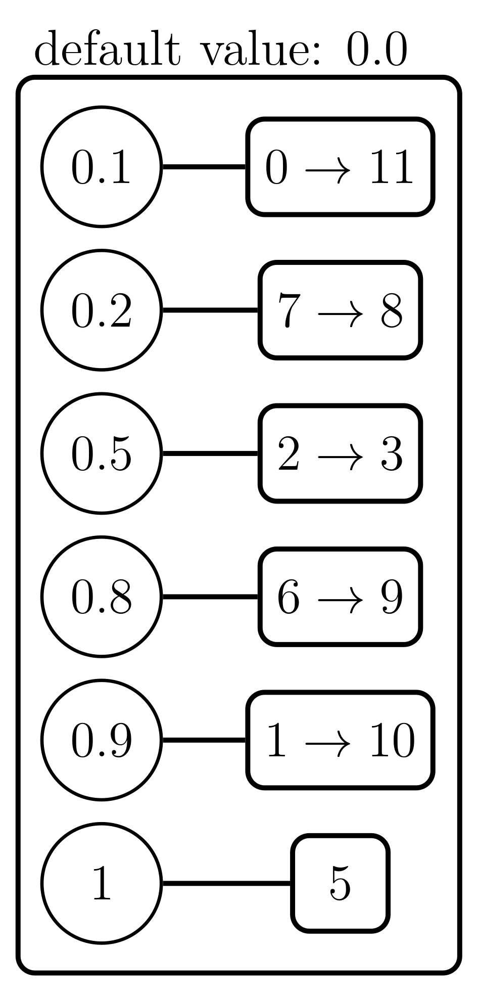
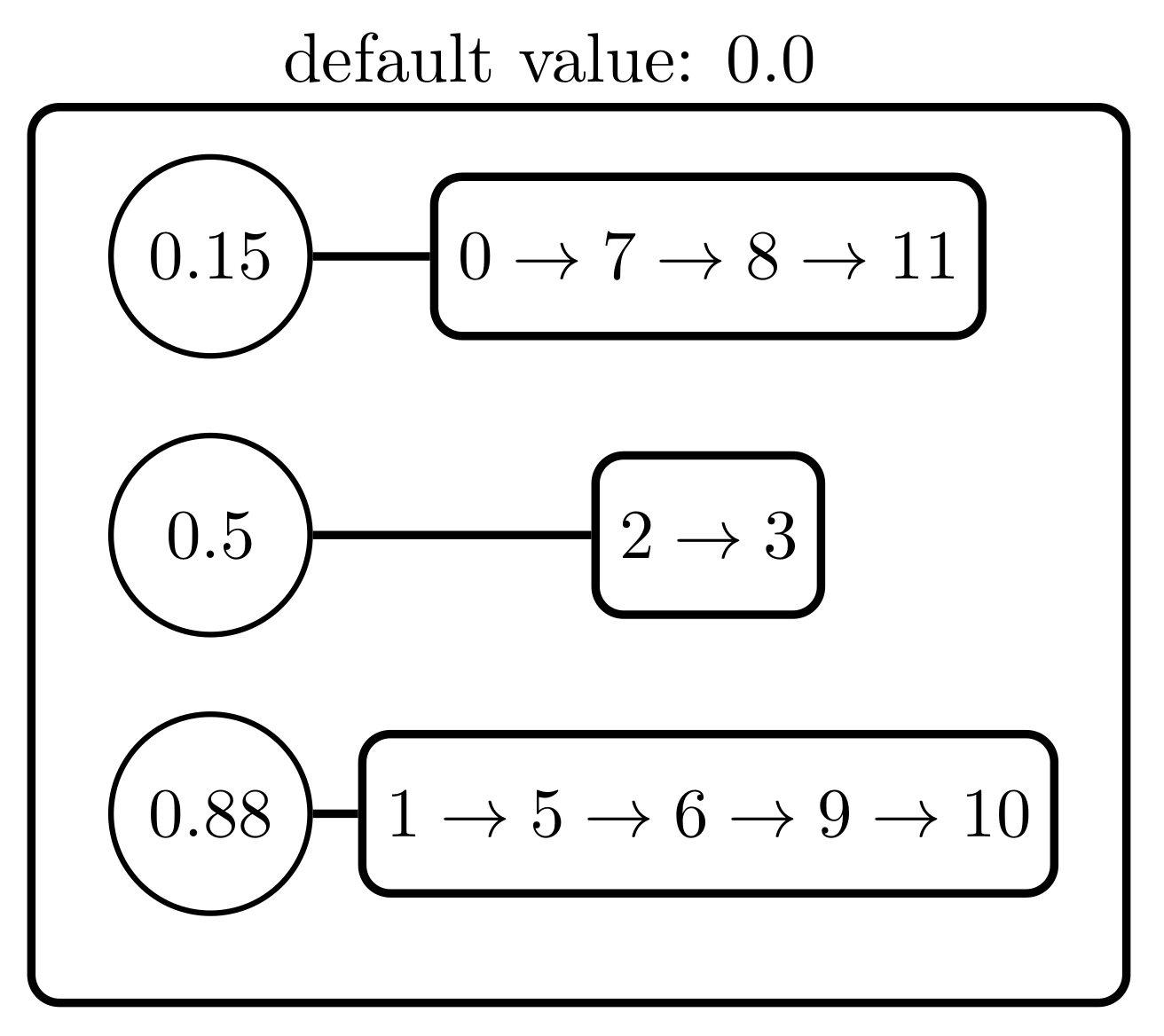
3.2. Alternative Structures: Value-Based Potentials

Valued-based potentials were recently introduced [16] as an alternative representation based exclusively on the values. Once such new structure was applied on several BNs from two different sources (bnlearn repository [17,18] and UAI competitions [19,20]) and compared with 1DAs, PTs, and PPTs. It has been proven that the use of VBP structures saves memory space. In VBPs, values must be stored paired with the indices (or configurations) that define the events in which they appear. How these pairs value-indices are stored determines two different VBP categories:

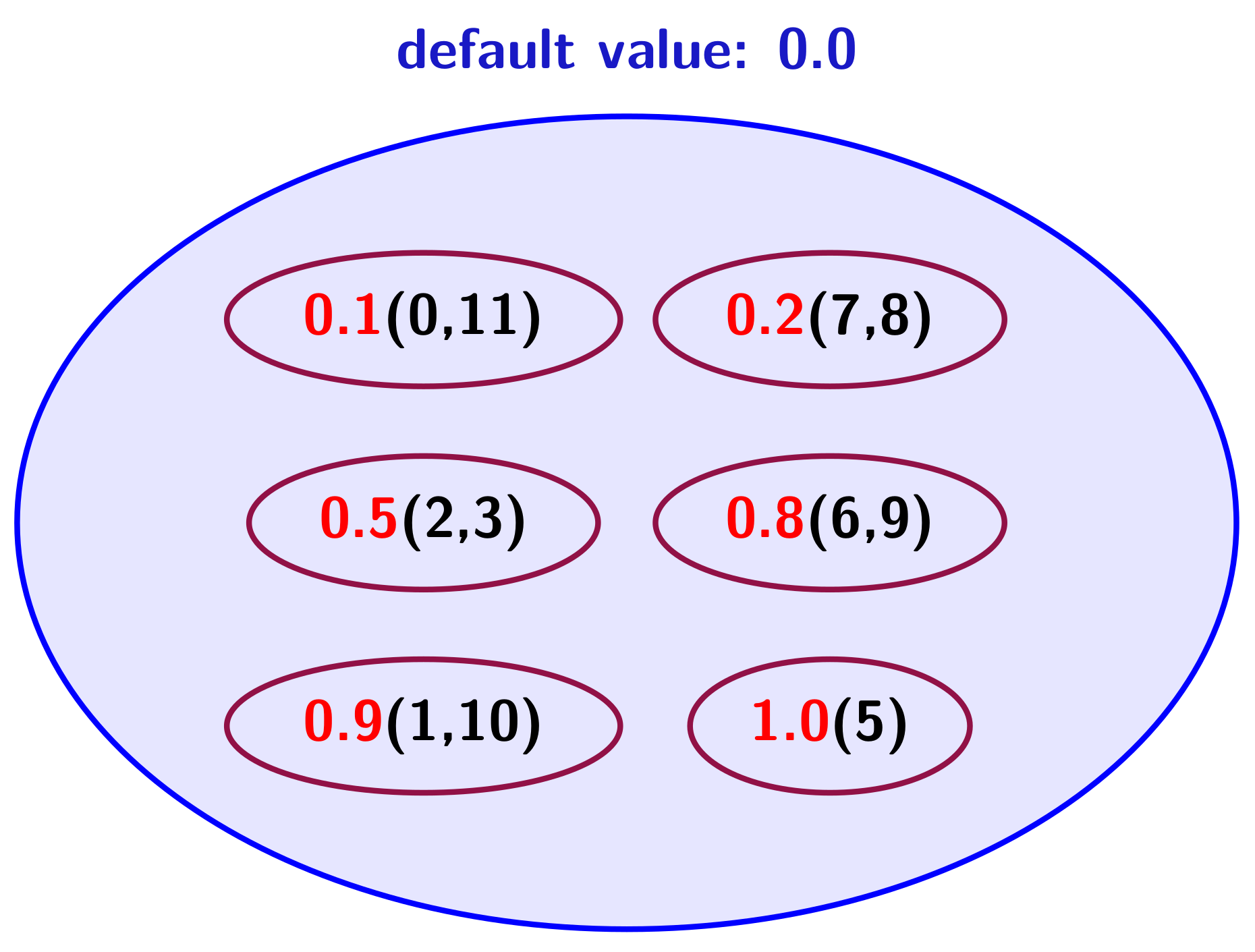
• Structures driven by values, using dictionaries in which the keys will be values: value-driven with grains (VDG) and value-driven with indices (VDI).
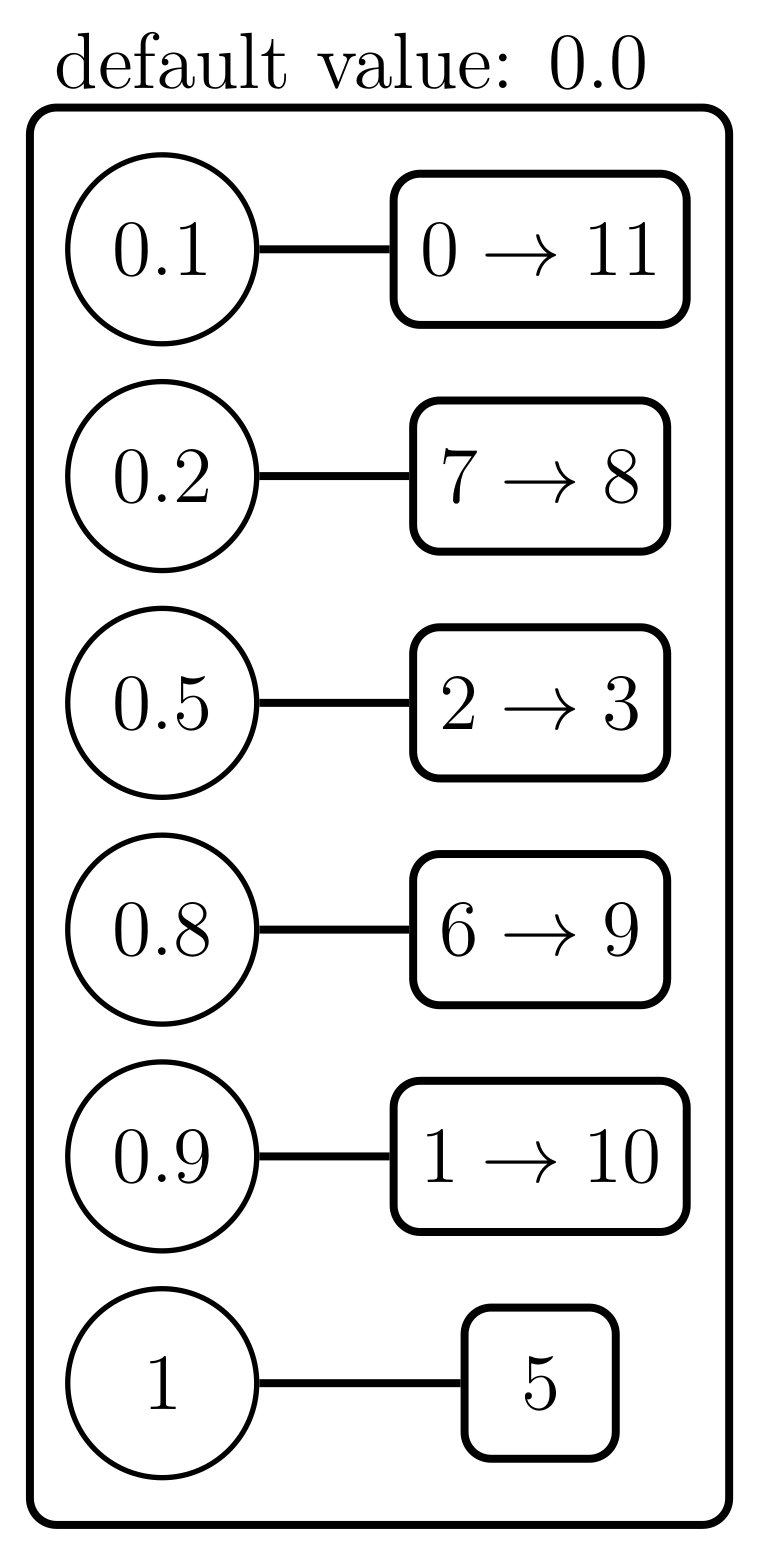
• Structures driven by indices, where keys are indices: index-driven with pair of arrays (IDP) and index-driven with map (IDM).

In all of these alternatives, a default value is set (in our case, $0.0$) and any related index will not be stored (in order to reduce memory space). Such a default value can be defined in advance or may be conveniently selected as the most repeated one. As VBPs represent potentials, it will be easy to adapt inference algorithms to use VBPs. A more complete definition of VBPs can be found in [16].

A simple visual idea of how VBPs work can be presented as a set of conveniently arranged probability values (i.e., each value is stored near its corresponding indices). Our studied example will appear as in Figure 6. It should be observed that the index 4, relating to value $0.0$ (the default value), is not stored at all. This would be similar to storing the values using a 1DA structure. However, the goal is to avoid storing duplicated values. The example shows how each of the values, $0.1$, $0.2$, $0.5$, $0.8$, and $0.9$, appear to be associated with two different indices (or configurations).

By using VBPs, therefore, each value is represented only once and all the indices in which it appears are linked to it. Figure 7 shows the groupings made and this highlights the fact that only 6 probability values are stored. The purpose of VBPs is therefore to make as many groups as different probability values exist to avoid repetitions and associate the related indices of configurations.

From the alternatives presented in [16], in this paper we will focus on value-driven with indices (VDI) and index-driven with pairs (IDP), since both of these performed extremely well on most of the studied BNs.

3.2.1. VDI: Value-Driven with Indices

Let us consider a certain potential $\varphi$ defined over $\mathbf{X}$. A VDI for $\varphi$, $VD{I}_{\varphi }$, is a dictionary D in which each entry $<v,L_v>$ contains a value (as the key) and a list of indices $L_v$, such that $\varphi \left(l\right)=v$, for each $l\in L_v$.

Example 7.

The potential $\varphi (X_1,X_2,X_3)$ used before and described in Figure 1 will be represented as VDI as shown in Figure 8. The outermost rectangle represents the dictionary and the entry keys (values) are drawn as circles. Keys give access to the index lists (inner rectangles with rounded corners). It can be seen that this dictionary faithfully represents the grouping of values shown in Figure 7 as an intuitive explanation of the purpose of VBP structures.

3.2.2. IDP: Index-Driven with Pair of Arrays

Let $\varphi$ be a potential defined over $\mathbf{X}$. A structure IDP representing $\varphi$, $IP{D}_{\varphi }$, is a pair of arrays V and L. Non-repeated values in $\varphi$ (excluding the default value) are stored in $V=\{v_0\dots v_{d-1}\}$. Let $n{d}_{\varphi }$ represent the number of indices storing non-default values. The array L is then defined as follows:

$$L:=\{(i,j):\varphi \left({\mathbf{x}}_i\right)=v_j,i\in n{d}_{\varphi }\}.$$

(5)

This means that IDP is based on two components: firstly, an array storing the values (without repetitions and excluding $0.0$ as the default value), and secondly, an array of pairs (index in potential, index in array of values). The second index of the pair saves the relationship between the indices and values.

Example 8.

The representation of potential $\varphi (X_1,X_2,X_3)$ as IDP is presented in Figure 9. The upper array (V) stores non-default values. The lower one includes pairs of indices. The fourth one $(3,2)$ represents the fact that $\varphi \left({\mathbf{x}}_3\right)=V\left(2\right)=0.5$.

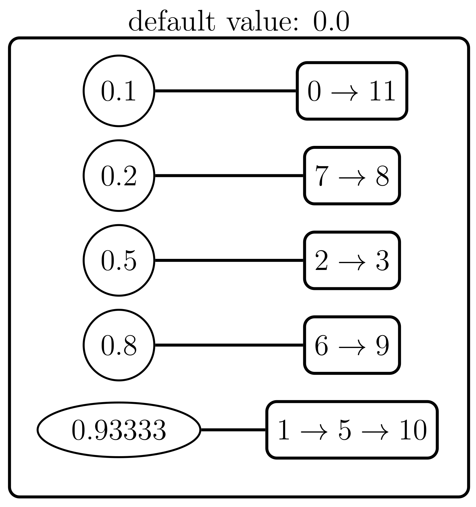
4. Approximating Value-Based Potentials

As we previously mentioned in Section 3, tables or 1DA were widely used in the bibliography to represent quantitative information in BNs or IDs. There is, however, a limitation of representing potentials with the 1DA structure and that is that they increase exponentially in size as the number of variables increases. Inferring or even dealing with these may therefore be (in the case of complex models) computationally unfeasible. For this purpose, it is convenient not only to define new structures which are able to compactly represent such potentials, but also methods to approximate them so that the memory space may be reduced without any significant loss of information. PTs can take advantage of context-specific independences, thereby reducing the number of stored values, but can also be approximated and so produce PPTs (this feature was presented as an additional advantage of PTs from their definition). However, the guiding procedure for the approach is computationally very expensive as it is necessary to determine the degree of information of each variable in order to ensure that the most informative ones appear as close as possible to the root. This ensures that the values stored in the tree leaves are most similar and, therefore, the loss of information is less when various values are replaced with their average value.

VBP structures [16] may produce a relevant decrease in the memory space when repeated values are present. Moreover, the approximation operation can be applied in a very simple way. This work presents an algorithm for this operation and also provides a theoretical justification for it. Our experimental work will show the performance of the algorithm using two different alternatives for VBPs: value-driven with indices (VDI) and index-driven with pairs (IDP).

4.1. Algorithm

The method to approximate a given potential $\varphi :{\mathsf{\Omega }}_{\mathbf{X}}\to {\mathbb{R}}_0^{+}$ is explained by considering potentials represented as VDI because this structure is simpler, but the practical application follows the same idea as for any other alternative (such as IDP, for example). Let the VBP potential to approximate be denoted as V. Let us assume that it stores n different values, denoted as $v_1\dots v_n$ in increasing order of size. As we mentioned in our description of VBPs, although each different value $v_i$ is only stored once, the information about the set of corresponding indices (or configurations) is saved, where ${\mathbf{S}}_i$ is $n_i=\left|{\mathbf{S}}_i\right|$ (which means that $n_i$ is the number of configurations in ${\mathbf{S}}_i$).

Definition 1.

The basic approximation step consists of reducing the number of values by applying a reduction operation. This operation replaces two consecutive values, $v_i$ and $v_{i+1}$, with their weighted average. Reduction can generally be described using the following notation:

• $v_a$ and $v_b$ will be the values to reduce with ${\mathbf{S}}_a$ and ${\mathbf{S}}_b$ as their sets of indices, with $n_a=\left|{\mathbf{S}}_a\right|$ and $n_b=\left|{\mathbf{S}}_b\right|$.
• $v_r$ is the new value that replaces $v_a$ and $v_b$, with ${\mathbf{S}}_r={\mathbf{S}}_a\cup {\mathbf{S}}_b$ and $n_r=\left|{\mathbf{S}}_r\right|$. This value is computed as:

  $$v_r={\displaystyle \frac{n_a·v_a+n_b·v_b}{n_a+n_b}}.$$
• It is important to observe that this operation does not modify the total sum of the potential values. Therefore, if ϕ is the original potential and V the result of successive reductions, then $sum\left(\varphi \right)=sum\left(V\right)$.

Consequently, at the end of this operation, the number of values is reduced. The complete algorithm employed for approximating $V_{\varphi }$ can now be intuitively described as follows:

1

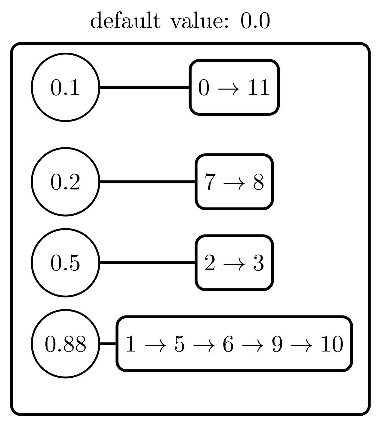
There are a number of different approximation alternatives resulting in candidate structures which will become the one chosen for the final approximation. As there are n different values, there will be $n-1$ candidate structures produced by reducing every pair of consecutive values. Iterate from $i=1$ to $i=n-1$:

1.1

Let us consider two successive values: $v_i$ and $v_{i+1}$. The candidate structure is then obtained by reducing both values as previously explained in Definition 1. The result of this operation will be $V_i$.

1.2

Calculate the Kullback–Leibler divergence between the original potential V and $V_i$. This value is denoted by $D(V,V_i)$.

2

Select the candidate structure $V_m=\underset{j=1\dots n-1}{argmin}D(V,V_j)$.

3

Repeat the previous steps until the selected stopping condition has been satisfied.

Before presenting a detailed description of the algorithm, we wish to include a number of considerations:

• It is evident that it is not necessary to build the candidate structures but only to evaluate the loss of information of the corresponding reduction operations.
• The Kullback–Leibler divergence between a candidate structure $V_i$ and the original one can be computed by taking into account only those values and indices involved in the reduction, and the measure to compute is in fact the loss of information produced by this operation. The way to compute this measure will be explained below.
• A possible stopping criteria (this is the one used in the experimental work although others could be considered) consists of setting a global information loss threshold, $t_l$. Therefore, the procedure of reducing consecutive values will continue as long as the addition of information losses does not reach the threshold $t_l$.

4.2. Theoretical Background

Let us consider a potential $\varphi \left(\mathbf{X}\right)$ where $V\left(\mathbf{X}\right)$ is its representation as VBP. The degree of approximation between them will be measured with the Kullback–Leibler divergence [21] between the corresponding normalized potentials ($\overline{\varphi }$ and $\overline{V}$):

$$D(\varphi ,V)=\sum _{\mathbf{x}\in {\mathsf{\Omega }}_{\mathbf{X}}}\overline{\varphi }\left(\mathbf{x}\right)log{\displaystyle \frac{\overline{\varphi }\left(\mathbf{x}\right)}{\overline{V}\left(\mathbf{x}\right)}}.$$

(6)

The divergence is a non-negative real number which would only be equal to zero if V provides an exact representation of $\varphi$. As we explained previously, the key operation for approximating $\varphi$ represented as V is reduction, as described in Definition 1 and Algorithm 1.

Algorithm 1: Approximation of a potential $\varphi$ represented as V (VBP).

1: functionApproximate($V,t_l$)        ▹$t_l$: global loss threshold 2:     loss ← 0 3:     while loss < tl do          ▹ loss threshold is not reached 4:         n← number of values in $\varphi$ 5:         for $i\in \{1,...,n-1\}$ do 6:            consider the reduction of $v_i$ and $v_{i+1}$ 7:            // compute information loss in V due to reduction 8:            compute $I(V,{\mathbf{S}}_i,{\mathbf{S}}_{i+1})$ 9:         end for 10:         choose $V_m$ which minimizes $I(V,{\mathbf{S}}_i,{\mathbf{S}}_{i+1}),i=1\dots n-1)$ 11:         loss ← loss + $I(V,{\mathbf{S}}_m,{\mathbf{S}}_{m+1})$ 12:         $V\leftarrow V_m$          ▹ keeps reducing V if possible 13:     end while 14:     return V        ▹ return V after reaching the loss threshold 15: end function

Definition 2.

Let us use $V_j$ to denote the approximated VBP structure obtained in the j-th iteration of the algorithm under consideration in the $j+1$-th iteration. The new reduction to consider will be described in the previously presented terms. The information loss produced by this reduction is defined as:

$$I(V_j,{\mathbf{S}}_a,{\mathbf{S}}_b)=D(\varphi ,V_j)-D(\varphi ,V_{j+1}).$$

(7)

The selection of the pair of values minimizing the information loss will consequently lead to the minimum value of the Kullback–Leibler divergence between the original potential and the approximate one.

Proposition 1.

The information loss obtained by reducing $v_a$ and $v_b$ in V can be computed as follows:

$$\begin{array}{c}I(V,{\mathbf{S}}_a,{\mathbf{S}}_b)={\displaystyle \frac{1}{sum\left(V\right)}}\left[log\left(v_r\right)sum\left(V^{\downarrow {\mathbf{S}}_r}\right)-log\left(v_a\right)sum\left(V^{\downarrow {\mathbf{S}}_a}\right)-log\left(v_b\right)sum\left(V^{\downarrow {\mathbf{S}}_b}\right)\right].\end{array}$$

(8)

where $sum\left(V\right)$ denotes the addition of every value of V and $V^{\downarrow \mathbf{S}}$ represents the potential V restricted to the configurations included in $\mathbf{S}$ and all remaining values are discarded. If we consider ϕ to be the original potential and V its representation as VBP (perhaps after applying several reduction operations), then $sum\left(\varphi \right)=sum\left(V\right)$ and the previous equation can be expressed as:

$$\begin{array}{c}I(V,{\mathbf{S}}_a,{\mathbf{S}}_b)={\displaystyle \frac{1}{sum\left(\varphi \right)}}\left[log\left(v_r\right)sum\left({\varphi }^{\downarrow {\mathbf{S}}_r}\right)-log\left(v_a\right)sum\left({\varphi }^{\downarrow {\mathbf{S}}_a}\right)-log\left(v_b\right)sum\left({\varphi }^{\downarrow {\mathbf{S}}_b}\right)\right].\end{array}$$

(9)

Proof .

Let ϕ be a potential represented by V (a VBP). $V_j$ denotes the potential obtained from V as a result of the j-th iteration of the approximation algorithm. According to Definition 2:

$$I(V_j,{\mathbf{S}}_a,{\mathbf{S}}_b)=D(\varphi ,V_j)-D(\varphi ,V_{j+1}).$$

(10)

This difference can be calculated by separating the configurations defined in $\mathbf{X}$ into three different subsets: ${\mathsf{\Omega }}_{\mathbf{X}}=\{{\mathsf{\Omega }}_{\mathbf{X}}\setminus {\mathbf{S}}_r\}\cup {\mathbf{S}}_a\cup {\mathbf{S}}_b$:

$$\begin{array}{c}I(V_j,{\mathbf{S}}_a,{\mathbf{S}}_b)=D(\varphi ,V_j)-D(\varphi ,V_{j+1})=\\ {\displaystyle \sum _{\mathbf{x}\in \{{\mathsf{\Omega }}_{\mathbf{X}}\setminus {\mathbf{S}}_r\}}}\left[\overline{\varphi }\left(\mathbf{x}\right)log\left({\displaystyle \frac{\overline{\varphi }\left(\mathbf{x}\right)}{{\overline{V}}_j\left(\mathbf{x}\right)}}\right)-\overline{\varphi }\left(\mathbf{x}\right)log\left({\displaystyle \frac{\overline{\varphi }\left(\mathbf{x}\right)}{{\overline{V}}_{j+1}\left(\mathbf{x}\right)}}\right)\right]+\\ {\displaystyle \sum _{\mathbf{x}\in {\mathbf{S}}_a}}\left[\overline{\varphi }\left(\mathbf{x}\right)log({\displaystyle \frac{\overline{\varphi }\left(\mathbf{x}\right)}{v_a/sum\left(\varphi \right))}}-\overline{\varphi }\left(\mathbf{x}\right)log\left({\displaystyle \frac{\overline{\varphi }\left(\mathbf{x}\right)}{v_r/sum\left(\varphi \right)}}\right)\right]+\\ {\displaystyle \sum _{\mathbf{x}\in {\mathbf{S}}_b}}\left[\overline{\varphi }\left(\mathbf{x}\right)log({\displaystyle \frac{\overline{\varphi }\left(\mathbf{x}\right)}{v_b/sum\left(\varphi \right))}}-\overline{\varphi }\left(\mathbf{x}\right)log\left({\displaystyle \frac{\overline{\varphi }\left(\mathbf{x}\right)}{v_r/sum\left(\varphi \right)}}\right)\right].\end{array}$$

(11)

It should be noted that the first part of the summation is equal to 0 since the values of the configurations that are not involved in the reduction ($\mathbf{x}\in {\mathsf{\Omega }}_{\mathbf{X}\setminus {\mathbf{S}}_r}$) are identical in $V_j$ and $V_{j+1}$. Additionally, when the properties of the logarithm are considered, the previous equation can be expressed as follows:

$$\begin{array}{c}{\displaystyle \sum _{\mathbf{x}\in {\mathbf{S}}_a}}\overline{\varphi }\left(\mathbf{x}\right)\left[log\left(\overline{\varphi }\left(\mathbf{x}\right)\right)-log\left({\displaystyle \frac{v_a}{sum\left(\varphi \right)}}\right)-log\left(\overline{\varphi }\left(\mathbf{x}\right)\right)+log\left({\displaystyle \frac{v_r}{sum\left(\varphi \right)}}\right)\right]+\\ {\displaystyle \sum _{\mathbf{x}\in {\mathbf{S}}_b}}\overline{\varphi }\left(\mathbf{x}\right)\left[log(\overline{\varphi }\left(\mathbf{x}\right)-log\left({\displaystyle \frac{v_b}{sum\left(\varphi \right)}}\right)-log\left(\overline{\varphi }\left(\mathbf{x}\right)\right)+log\left({\displaystyle \frac{v_r}{sum\left(\varphi \right)}}\right)\right]=\\ {\displaystyle \sum _{\mathbf{x}\in {\mathbf{S}}_a}}\overline{\varphi }\left(\mathbf{x}\right)log\left({\displaystyle \frac{v_r}{v_a}}\right)+{\displaystyle \sum _{\mathbf{x}\in {\mathbf{S}}_b}}\overline{\varphi }\left(\mathbf{x}\right)log\left({\displaystyle \frac{v_r}{v_b}}\right).\end{array}$$

(12)

Since $\overline{\varphi }\left(\mathbf{x}\right)={\displaystyle \frac{\varphi \left(\mathbf{x}\right)}{sum\left(\varphi \right)}}$ and if we remove the logarithm from the sum as it does not depend on the configurations, the previous equation can then be written as follows:

$$\begin{array}{c}log\left({\displaystyle \frac{v_r}{v_a}}\right){\displaystyle \sum _{\mathbf{x}\in {\mathbf{S}}_a}}{\displaystyle \frac{\varphi \left(\mathbf{x}\right)}{sum\left(\varphi \right)}}+log\left({\displaystyle \frac{v_r}{v_b}}\right){\displaystyle \sum _{\mathbf{x}\in {\mathbf{S}}_b}}{\displaystyle \frac{\varphi \left(\mathbf{x}\right)}{sum\left(\varphi \right)}}=\\ {\displaystyle \frac{1}{sum\left(\varphi \right)}}\left[log\left(v_r\right)sum\left({\varphi }^{\downarrow {\mathbf{S}}_a}\right)-log\left(v_a\right)sum\left({\varphi }^{\downarrow {\mathbf{S}}_a}\right)+log\left(v_r\right)sum\left({\varphi }^{\downarrow {\mathbf{S}}_b}\right)-log\left(v_b\right)sum\left({\varphi }^{\downarrow {\mathbf{S}}_b}\right)\right]=\\ {\displaystyle \frac{1}{sum\left(\varphi \right)}}\left[log\left(v_r\right)sum\left({\varphi }^{\downarrow {\mathbf{S}}_r}\right)-log\left(v_a\right)sum\left({\varphi }^{\downarrow {\mathbf{S}}_a}\right)-log\left(v_b\right)sum\left({\varphi }^{\downarrow {\mathbf{S}}_b}\right)\right].\end{array}$$

(13)

4.3. Example

The application of the approximation algorithm will be exemplified using the potential presented in Example 1 and stored as a VDI, as shown in Figure 10. The practical implementation of the algorithm attempts to simplify computations as much as possible. Therefore, the global sum of the potential values in Equation (8) can be avoided, as it is not needed for determining the candidate structure with lower loss of information.

As the potential stores 6 different probability values, the initial iteration must therefore consider 5 candidate structures, i.e., 5 different reduction operations, and then calculate their respective information losses. This information is presented in

Table 1. Candidate structures for the first iteration. Bold typeface is used for the preferred candidate structure.

${\mathit{v}}_{\mathit{a}}\mathbf{-}{\mathbf{S}}_{\mathit{a}}$	${\mathit{v}}_{\mathit{b}}\mathbf{-}{\mathbf{S}}_{\mathit{b}}$	${\mathit{v}}_{\mathit{r}}\mathbf{-}{\mathbf{S}}_{\mathit{r}}$	$\mathit{I}\mathbf{(}\mathit{V}\mathbf{,}{\mathbf{S}}_{\mathit{a}}\mathbf{,}{\mathbf{S}}_{\mathit{b}}\mathbf{)}$
$0.1-\{0,11\}$	$0.2-\{7,8\}$	$0.15-\{0,7,8,11\}$	$0.014757$
$0.2-\{7,8\}$	$0.5-\{2,3\}$	$0.35-\{2,3,7,8\}$	$0.057686$
$0.5-\{2,3\}$	$0.8-\{6,9\}$	$0.65-\{2,3,6,9\}$	$0.030339$
$0.8-\{6,9\}$	$0.9-\{1,10\}$	$0.85-\{1,6,9,10\}$	$0.002556$
$\mathbf{0.9}\mathbf{-}\mathbf{\{}\mathbf{1}\mathbf{,}\mathbf{10}\mathbf{\}}$	$\mathbf{1}\mathbf{-}\mathbf{\left\{}\mathbf{5}\mathbf{\right\}}$	$\mathbf{0.93333}\mathbf{-}\mathbf{\{}\mathbf{1}\mathbf{,}\mathbf{5}\mathbf{,}\mathbf{10}\mathbf{\}}$	$\mathbf{0.001533}$

. Each row considers the values to be reduced ($v_a$ and $v_r$) and the new value ($v_r$) in addition to their corresponding sets of indices (${\mathbf{S}}_a$, ${\mathbf{S}}_b$ and ${\mathbf{S}}_r$). The alternative with the lowest information loss is presented in bold.

Therefore, the preferred candidate structure is the final one and the resulting approximate structure is the one presented in Figure 11. The total loss is $0.001533$.

In the second iteration, there are only 4 candidate structures to consider, as shown in

Table 2. Candidate structures for the second iteration. The best reduction is presented with bold typeface.

${\mathit{v}}_{\mathit{a}}\mathbf{-}{\mathbf{S}}_{\mathit{a}}$	${\mathit{v}}_{\mathit{b}}\mathbf{-}{\mathbf{S}}_{\mathit{b}}$	${\mathit{v}}_{\mathit{r}}\mathbf{-}{\mathbf{S}}_{\mathit{r}}$	$\mathit{I}\mathbf{(}\mathit{V}\mathbf{,}{\mathbf{S}}_{\mathit{a}}\mathbf{,}{\mathbf{S}}_{\mathit{b}})$
$0.1-\{0,11\}$	$0.2-\{7,8\}$	$0.15-\{0,7,8,11\}$	$0.014757$
$0.2-\{7,8\}$	$0.5-\{2,3\}$	$0.35-\{2,3,7,8\}$	$0.057686$
$0.5-\{2,3\}$	$0.8-\{6,9\}$	$0.65-\{2,3,6,9\}$	$0.030339$
$\mathbf{0.8}-\{\mathbf{6},\mathbf{9}\}$	$\mathbf{0.93333}-\{\mathbf{1},\mathbf{5},\mathbf{10}\}$	$\mathbf{0.88}-\{\mathbf{1},\mathbf{5},\mathbf{6},\mathbf{9},\mathbf{10}\}$	$\mathbf{0.005323}$

.

The reduction of the values $0.8$ and $0.93333$ therefore performs the best. The approximate structure after this iteration is presented in Figure 12. The global loss is now $0.006856$.

In the next step, we will consider a third iteration by selecting from among the candidate reductions presented in

Table 3. Candidate structures for the third iteration. The best reduction is presented with bold typeface.

${\mathit{v}}_{\mathit{a}}\mathbf{-}{\mathbf{S}}_{\mathit{a}}$	${\mathit{v}}_{\mathit{b}}\mathbf{-}{\mathbf{S}}_{\mathit{b}}$	${\mathit{v}}_{\mathit{r}}\mathbf{-}{\mathbf{S}}_{\mathit{r}}$	$\mathit{I}\mathbf{(}\mathit{V}\mathbf{,}{\mathbf{S}}_{\mathit{a}}\mathbf{,}{\mathbf{S}}_{\mathit{b}}\mathbf{)}$
$\mathbf{0.1}\mathbf{-}\mathbf{\{}\mathbf{0}\mathbf{,}\mathbf{11}\mathbf{\}}$	$\mathbf{0.2}\mathbf{-}\mathbf{\{}\mathbf{7}\mathbf{,}\mathbf{8}\mathbf{\}}$	$\mathbf{0.15}\mathbf{-}\mathbf{\{}\mathbf{0}\mathbf{,}\mathbf{7}\mathbf{,}\mathbf{8}\mathbf{,}\mathbf{11}\mathbf{\}}$	$\mathbf{0.014757}$
$0.2-\{7,8\}$	$0.5-\{2,3\}$	$0.35-\{2,3,7,8\}$	$0.057686$
$0.5-\{2,3\}$	$0.88-\{1,5,6,9,10\}$	$0.65-\{2,3,6,9\}$	$0.063298$

.

If we combine the values $0.1$ and $0.2$, we obtain the new approximated potential shown in Figure 13.

The loss of information in relation to the original potential is now $0.021613$. The next iteration must select between only two reductions, as shown in

Table 4. Candidate structures for the fourth iteration.

${\mathit{v}}_{\mathit{a}}\mathbf{-}{\mathbf{S}}_{\mathit{a}}$	${\mathit{v}}_{\mathit{b}}\mathbf{-}{\mathbf{S}}_{\mathit{b}}$	${\mathit{v}}_{\mathit{r}}\mathbf{-}{\mathbf{S}}_{\mathit{r}}$	$\mathit{I}\mathbf{(}\mathit{V}\mathbf{,}{\mathbf{S}}_{\mathit{a}}\mathbf{,}{\mathbf{S}}_{\mathit{b}}\mathbf{)}$
$0.15-\{0,7,8,11\}$	$0.5-\{2,3\}$	$0.5333-\{0,2,3,7,8,11\}$	$0.123074$
$0.5-\{2,3\}$	$0.88-\{1,5,6,9,10\}$	$0.65-\{2,3,6,9\}$	$0.063298$

.

If the global loss threshold is $0.05$, then there are no more reductions to apply and the process ends with the approximate potential shown in Figure 13. We need to make one last comment about the operation of the algorithm. If we look at the tables, it is apparent that information loss values for each reduction remain constant, regardless of the other values. This facilitates the consideration of alternative structures by storing the already calculated loss values, thereby avoiding repeated computations.

5. Empirical Evaluation

The application of the approximation algorithm will be evaluated by considering various BNs developed for modeling medical problems. All of these are included in the bnlearn repository (see [17,18]) and are either categorized as large (HEPAR II) or very large (diabetes, munin, and pathfinder) networks. The main features of these are described below.

• The hepar2 network was defined by A. Onisko in her Ph.D. dissertation [22] as part of the HEPAR II project. The project was inspired by the HEPAR system [23], the aim of which is to support the diagnosis of liver and biliary tract disorders.
• pathfinder [24] is a system which, when combined with expert knowledge from surgical pathologists, can assist in the diagnosis of lymphnode diseases. As a result of this study, the discrete pathfinder network was defined.
• The munin network was defined while creating the expert system identified by the same acronym MUNIN (MUscle and Nerve Inference Network) [25]. The aim of this system was to help electromyographics (EMCs), which are designed to localize and characterize lesions of the neuro-muscular system, from a patho-physiological approach combined with expert knowledge.
• The diabetes [26] BN represents a differential equation model which attempts to adjust the insulin therapy for diabetic people. The model considers the patient’s state by measuring blood glucose, biologically active insulin, and the amount of undigested carbohydrate within an hour gap in addition to other known variables involved in the glucose metabolism process. The diabetes network enabled predictions to be extended to 24-h blood glucose profiles and the insulin treatment to be adjusted.

Table 5. Bayesian network features.

Network	Nodes	arcs	np	avg. M.B. Size	avg. deg	Max. in-deg
hepar2	70	123	2139	4.51	3.51	6
pathfinder	223	338	97,851	5.61	3.03	6
munin	1041	1397	98,423	3.54	2.68	3
diabetes	413	606	461,069	3.97	2.92	2

presents a summary of the information for each network: number of nodes, number of arcs, number of parameters ($np$), average Markov blanket (M.B.) size, average degree, and maximum in-degree. The networks are ordered according to the number of parameters because this is the most relevant feature in terms of the experimental work.

The experimental section is organized in the following way:

1.

Analysis of the memory space necessary to store the complete networks using the different representation alternatives in order to compare it with the representation using 1DA, since this is considered to be the base representation (see Section 5.1).

2.

Analysis of the main characteristics of the specific potentials of some variables that will later be used to perform inference, as well as the memory space necessary for their representation with the different structures considered (see Section 5.2).

3.

Examination of the effect of the approximation on the memory space necessary for the storage of each network (see Section 5.3). The relationship with the memory space required by the base representation is determined, as well as the reduction produced in relation to the alternative representations but without any approximation. In this case, the results are presented by means of a specific table for each network in order to collect the information on the threshold values considered.

4.

Propagation errors produced by the approximation, both local (only the potential of the target variable is approximated) and global (all potentials are approximated) (see Section 5.4). A table is presented for each network and this collects the results for the selected variables and for the set of thresholds used.

5.

In order to obtain further information about the effect of the approximation, some charts are also included to show the effect of the approximation on the order of the probabilities of the marginal distributions obtained as a result of the propagation. If these distributions are used to make decisions, it is important that the alternatives are kept in the same order (according to their probability value) in which they appear in the exact result, without approximation (see Section 5.5).

5.1. Global Memory Size Analysis

This section analyzes the networks in order to determine the necessary memory size for each form of representation being considered: 1DA, PT, PPT, VDI, and IPD. This part serves to check the convenience of using alternative VBP-type representations in networks modeling real-world medical problems. In this way, a base memory size is available and it will enable the effect of the approximation on memory spaces required for the VBP-type representations to be subsequently checked. Table 6 includes the following information:

• network: name of the network;
• 1DA: memory size indispensable for 1DA storing the complete set of potentials;
• PT: memory size required for PT representation and the saving or increase in space in terms of 1DA. This last value is included in the second line and is computed as

  $${\displaystyle \frac{as*100}{bs}}-100,$$

  (14)
• where $as$ refers to the memory size of the alternative representation, and $bs$ to the memory size of the 1DA representation;
• PPT, VDI, and IDP: the same as the previous line for the remaining representations: pruned probability trees, VDI and IDP.

In Table 6, the best savings values are shown in bold. The results show that VBP structures behave better than PT and PPT in every network, although in some of these there are no savings in terms of the space required for the simplest representation of all: 1DA. Some more specific comments are included below:

• In hepar2, we can see that PPT offers little improvement in relation to PT, which indicates that in reality there are few repeated values that can be used by the PPT pruning operation. The VDI structure provides a saving of approximately $44\%$ compared to PT, while IPD represents a saving of $62\%$.
• In the case of pathfinder, there are notable savings in relation to 1DA and very important ones with respect to PT and PPT. The biggest savings come from the VDI structure.
• With respect to the munin network, VDI representation needs almost the same memory space as 1DA and there is a saving of about $23\%$ in IDP (moreover, significant reductions can also be seen with respect to PT and PPT).
• Finally, for diabetes, both VBP structures represent a substantial reduction in memory space and this is slightly greater in the case of VDI.

Table 6. Global memory size analysis. Bold typeface denotes the structure with the best saving percentage (or with the smallest increase percentage).

Network	1DA	PT	PPT	VDI	IDP
hepar2	32,530	132,026	131,756	74,070	49,602
		305.8592	305.0292	127.6975	52.4808
pathfinder	806,982	4,249,768	3,779,470	301,602	482,438
		426.6249	368.3463	$\mathbf{-}\mathbf{62.6259}$	−40.2170
munin	994,672	3,393,878	3,353,900	997,864	766,072
		241.2057	237.1865	0.3209	$\mathbf{-}\mathbf{22.9825}$
diabetes	3,773,200	10,044,948	10,044,810	964,380	1,105,728
		166.2183	166.2146	$\mathbf{-}\mathbf{74.4413}$	−70.6952

Table 6. Global memory size analysis. Bold typeface denotes the structure with the best saving percentage (or with the smallest increase percentage).

Network	1DA	PT	PPT	VDI	IDP
hepar2	32,530	132,026	131,756	74,070	49,602
		305.8592	305.0292	127.6975	52.4808
pathfinder	806,982	4,249,768	3,779,470	301,602	482,438
		426.6249	368.3463	$\mathbf{-}\mathbf{62.6259}$	−40.2170
munin	994,672	3,393,878	3,353,900	997,864	766,072
		241.2057	237.1865	0.3209	$\mathbf{-}\mathbf{22.9825}$
diabetes	3,773,200	10,044,948	10,044,810	964,380	1,105,728
		166.2183	166.2146	$\mathbf{-}\mathbf{74.4413}$	−70.6952

In short, these data show the capacity of these structures to offer efficient mechanisms for representing quantitative information, and, as will be seen below, they allow the use of the approximation operation with the possibility of achieving additional memory savings.

5.2. Local Memory Size Analysis

This experiment gathers information about the selected variables of each network in order to determine their features and verify the relationship between representation and memory size. These variables will later be used as target variables using the VE algorithm [27,28,29] to compute their marginal distributions. The columns included in Table 7 are:

• network: name of the network;
• variable: name of the variable being examined;
• np: global number of parameters of the target variable potential;
• nd: number of different values in the potential (these are the values actually stored in the VBP representation);
• 1DA: memory size for the 1DA representation;
• PT: memory size required for PT representation and saving or increase regarding 1DA. This last value is included in the second line and computed as before;
• PPT, VDI, and IDP: the same as the previous line for PPT, VDI, and IDP.

In this experiment, we have selected the variables with the largest number of parameters: hepar2 (ggtp, ast, alt, and bilirubin); pathfinder (F39, F74, and F40); munin (v1 (L_LNLPC5_DELT_MUSIZE), v2 (L_LNLE_ADM_MUSIZE), and v3 (L_MED_ALLCV_EW)); and diabetes (cho_0, cho_1, and cho_2). The best savings values are shown in bold. We wish to make the following comments about the results in Table 7:

• In hepar2 variables, the number of different probability values is slightly lower than the number of parameters. This justifies the fact that memory space requirements do not reduce those required by 1DA, although they do offer significant savings with respect to PT and PPT.
• Selected pathfinder variables present a high degree of repetition, so the number of different values is significantly lower than the number of parameters. This produces very significant memory savings in relation to 1DA which are larger in the case of VDI.
• For the first two munin variables, there are only 12 different values but 600 parameters. This accounts for the notable memory space savings for VBP structures. In the case of the third variable, there are more different values (133), although this does suppose a high degree of repetition compared to the 600 necessary parameters.
• Diabetes variables have similar characteristics: only 45 different values (and 7056 possible values). Consequently, the memory space savings are very noticeable and appreciably better in the case of VDI.

Table 7. Local memory size analysis. Numbers in bold typeface denotes the best saving percentages (or with the smallest increase percentage).

Network	Variable	np	nd	1DA	PT	PPT	VDI	IDP
hepar2	ggtp	384	334	3454	19,452 463.1731	19,452 463.1731	9990 189.2299	6150 78.0544
	ast	288	231	2636	13,648 417.7542	13,648 417.7542	7084 168.7405	4508 71.0167
	alt	288	249	2636	13,648 417.7542	13,648 417.7542	7516 185.1290	4652 76.4795
	bilirubin	288	244	2636	13,426 409.3323	13,426 409.3323	7396 180.5766	4612 74.9621
pathfinder	F39	8064	30	64,794	376,442 480.9828	359,850 455.3755	15,114 −76.6738	28,698 −55.7089
	F74	7560	111	60,712	293,736 383.8187	152,072 150.4810	28,676 −52.7672	52,632 −13.3087
	F40	4032	43	32,488	116,076 257.2888	114,588 252.7087	5640 −82.6397	9280 −71.4356
munin	v1	600	12	5032	19,132 280.2067	19,132 280.2067	1112 −77.9014	1464 −70.9062
	v2	600	12	5032	19,132 280.2067	19,132 280.2067	1112 −77.9014	1464 −70.9062
	v3	600	133	4982	15,012 201.3248	15,012 201.3248	4066 −18.3862	2582 −48.1734
diabetes	cho_0	7056	45	56,630	139,546 146.4171	139,546 146.4171	9454 −83.3057	16,878 −70.1960
	cho_1	7056	45	56,630	139,546 146.4171	139,546 146.4171	9454 −83.3057	16,878 −70.1960
	cho_2	7056	45	56,630	139,546 146.4171	139,546 146.4171	9454 −83.3057	16,878 −70.1960

Table 7. Local memory size analysis. Numbers in bold typeface denotes the best saving percentages (or with the smallest increase percentage).

Network	Variable	np	nd	1DA	PT	PPT	VDI	IDP
hepar2	ggtp	384	334	3454	19,452 463.1731	19,452 463.1731	9990 189.2299	6150 78.0544
	ast	288	231	2636	13,648 417.7542	13,648 417.7542	7084 168.7405	4508 71.0167
	alt	288	249	2636	13,648 417.7542	13,648 417.7542	7516 185.1290	4652 76.4795
	bilirubin	288	244	2636	13,426 409.3323	13,426 409.3323	7396 180.5766	4612 74.9621
pathfinder	F39	8064	30	64,794	376,442 480.9828	359,850 455.3755	15,114 −76.6738	28,698 −55.7089
	F74	7560	111	60,712	293,736 383.8187	152,072 150.4810	28,676 −52.7672	52,632 −13.3087
	F40	4032	43	32,488	116,076 257.2888	114,588 252.7087	5640 −82.6397	9280 −71.4356
munin	v1	600	12	5032	19,132 280.2067	19,132 280.2067	1112 −77.9014	1464 −70.9062
	v2	600	12	5032	19,132 280.2067	19,132 280.2067	1112 −77.9014	1464 −70.9062
	v3	600	133	4982	15,012 201.3248	15,012 201.3248	4066 −18.3862	2582 −48.1734
diabetes	cho_0	7056	45	56,630	139,546 146.4171	139,546 146.4171	9454 −83.3057	16,878 −70.1960
	cho_1	7056	45	56,630	139,546 146.4171	139,546 146.4171	9454 −83.3057	16,878 −70.1960
	cho_2	7056	45	56,630	139,546 146.4171	139,546 146.4171	9454 −83.3057	16,878 −70.1960

5.3. Global Memory Size with Approximation

This experiment considers the effect of the approximation on every potential in the network in terms of the necessary memory space after approximating with different thresholds. This determines the degree to which the approximation enables a reduction in the memory size for storing the networks. The results for this section are divided into various tables, one for each network (Table 8, Table 9, Table 10 and Table 11), and all have a similar structure.

• The first column shows the threshold.
• The second presents data relating to the VDI structure: memory size after approximation, savings over 1DA and savings with respect to the exact VDI representation.
• The third column is identical to the second but with data for the IDP structure.

5.3.1. hepar2 Network

The number of parameters is 2139, and the memory sizes of 1DA, PT, and PPT structures are 32,530, 132,026, and 131,756, respectively. Table 8 includes savings when approximation is applied.

Table 8. hepar2—Global approximation memory size analysis.

Threshold	VDI	IDP
0.00001	63,846 (96.2681/−13.8032)	46,194 (42.0043/−6.8707)
0.00005	58,062 (78.4875/−21.6120)	44,266 (36.0775/−10.7576)
0.00010	55,302 (70.0031/−25.3382)	43,346 (33.2493/−12.6124)
0.00050	48,558 (49.2714/−34.4431)	41,098 (26.3388/−17.1445)
0.00100	45,678 (40.4181/−38.3313)	40,138 (23.3876/−19.0799)
0.00500	39,798 (22.3425/−46.2697)	38,178 (17.3624/−23.0313)
0.01000	37,518 (15.3335/−49.3479)	37,418 (15.0261/−24.5635)
0.05000	33,798 (3.8979/−54.3702)	36,178 (11.2143/−27.0634)
0.10000	32,550 (0.0615/−56.0551)	35,762 (9.9354/−27.9021)

Table 8. hepar2—Global approximation memory size analysis.

Threshold	VDI	IDP
0.00001	63,846 (96.2681/−13.8032)	46,194 (42.0043/−6.8707)
0.00005	58,062 (78.4875/−21.6120)	44,266 (36.0775/−10.7576)
0.00010	55,302 (70.0031/−25.3382)	43,346 (33.2493/−12.6124)
0.00050	48,558 (49.2714/−34.4431)	41,098 (26.3388/−17.1445)
0.00100	45,678 (40.4181/−38.3313)	40,138 (23.3876/−19.0799)
0.00500	39,798 (22.3425/−46.2697)	38,178 (17.3624/−23.0313)
0.01000	37,518 (15.3335/−49.3479)	37,418 (15.0261/−24.5635)
0.05000	33,798 (3.8979/−54.3702)	36,178 (11.2143/−27.0634)
0.10000	32,550 (0.0615/−56.0551)	35,762 (9.9354/−27.9021)

Table 9. pathfinder—Global approximation memory size analysis.

Threshold	VDI	IDP
0.00001	293,178 (−63.6698/−2.7931)	479,630 (−40.5650/−0.5820)
0.00005	290,682 (−63.9791/−3.6207)	478,798 (−40.6681/−0.7545)
0.00010	289,266 (−64.1546/−4.0902)	478,326 (−40.7266/−0.8523)
0.00050	285,450 (−64.6275/−5.3554)	477,054 (−40.8842/−1.1160)
0.00100	283,170 (−64.9100/−6.1114)	476,294 (−40.9784/−1.2735)
0.00500	277,002 (−65.6743/−8.1564)	474,238 (−41.2331/−1.6997)
0.01000	274,050 (−66.0401/−9.1352)	473,254 (−41.3551/−1.9037)
0.05000	267,090 (−66.9026/−11.4429)	470,934 (−41.6426/−2.3846)
0.10000	264,450 (−67.2298/−12.3182)	470,054 (−41.7516/−2.5670)

Table 9. pathfinder—Global approximation memory size analysis.

Threshold	VDI	IDP
0.00001	293,178 (−63.6698/−2.7931)	479,630 (−40.5650/−0.5820)
0.00005	290,682 (−63.9791/−3.6207)	478,798 (−40.6681/−0.7545)
0.00010	289,266 (−64.1546/−4.0902)	478,326 (−40.7266/−0.8523)
0.00050	285,450 (−64.6275/−5.3554)	477,054 (−40.8842/−1.1160)
0.00100	283,170 (−64.9100/−6.1114)	476,294 (−40.9784/−1.2735)
0.00500	277,002 (−65.6743/−8.1564)	474,238 (−41.2331/−1.6997)
0.01000	274,050 (−66.0401/−9.1352)	473,254 (−41.3551/−1.9037)
0.05000	267,090 (−66.9026/−11.4429)	470,934 (−41.6426/−2.3846)
0.10000	264,450 (−67.2298/−12.3182)	470,054 (−41.7516/−2.5670)

Table 10. munin—Global approximation memory size analysis.

Threshold	VDI	IDP
0.00001	880,744 (−11.4538/−11.7371)	727,032 (−26.9074/−5.0961)
0.00005	829,096 (−16.6463/−16.9129)	709,816 (−28.6382/−7.3434)
0.00010	800,584 (−19.5128/−19.7702)	700,312 (−29.5937/−8.5840)
0.00050	725,440 (−27.0674/−27.3007)	675,264 (−32.1119/−11.8537)
0.00100	692,296 (−30.3996/−30.6222)	664,216 (−33.2226/−13.2959)
0.00500	615,976 (−38.0725/−38.2705)	638,776 (−35.7802/−16.6167)
0.01000	587,848 (−40.9003/−41.0894)	629,400 (−36.7229/−17.8406)
0.05000	533,728 (−46.3413/−46.5130)	611,360 (−38.5365/−20.1955)
0.10000	518,272 (−47.8952/−48.0619)	606,208 (−39.0545/−20.8680)

Table 10. munin—Global approximation memory size analysis.

Threshold	VDI	IDP
0.00001	880,744 (−11.4538/−11.7371)	727,032 (−26.9074/−5.0961)
0.00005	829,096 (−16.6463/−16.9129)	709,816 (−28.6382/−7.3434)
0.00010	800,584 (−19.5128/−19.7702)	700,312 (−29.5937/−8.5840)
0.00050	725,440 (−27.0674/−27.3007)	675,264 (−32.1119/−11.8537)
0.00100	692,296 (−30.3996/−30.6222)	664,216 (−33.2226/−13.2959)
0.00500	615,976 (−38.0725/−38.2705)	638,776 (−35.7802/−16.6167)
0.01000	587,848 (−40.9003/−41.0894)	629,400 (−36.7229/−17.8406)
0.05000	533,728 (−46.3413/−46.5130)	611,360 (−38.5365/−20.1955)
0.10000	518,272 (−47.8952/−48.0619)	606,208 (−39.0545/−20.8680)

Here are some comments about Table 8:

• For VDI, it is apparent that there is a very noticeable increase in memory space savings as the threshold used for the approximation becomes greater, reaching very similar sizes to those of 1DA for the threshold 0.1. For every threshold, there is a reduction in relation to the exact VDI structure (without the use of approximation).
• With the IDP structure, the behavior is similar, although the reductions are not as notable as with VDI.

Table 11. diabetes—Global approximation memory size analysis.

Threshold	VDI	IDP
0.00001	843,180 (−77.6535/−12.5677)	1,065,328 (−71.7659/−3.6537)
0.00005	799,932 (−78.7996/−17.0522)	1,050,912 (−72.1480/−4.9575)
0.00010	776,868 (−79.4109/−19.4438)	1,043,224 (−72.3517/−5.6527)
0.00050	719,148 (−80.9406/−25.4290)	1,023,984 (−72.8617/−7.3928)
0.00100	694,908 (−81.5831/−27.9425)	1,015,904 (−73.0758/−8.1235)
0.00500	644,076 (−82.9302/−33.2135)	998,960 (−73.5249/−9.6559)
0.01000	626,172 (−83.4047/−35.0700)	992,992 (−73.6830/−10.1956)
0.05000	594,324 (−84.2488/−38.3724)	982,376 (−73.9644/−11.1557)
0.10000	585,636 (−84.4791/−39.2733)	979,480 (−74.0411/−11.4176)

Table 11. diabetes—Global approximation memory size analysis.

Threshold	VDI	IDP
0.00001	843,180 (−77.6535/−12.5677)	1,065,328 (−71.7659/−3.6537)
0.00005	799,932 (−78.7996/−17.0522)	1,050,912 (−72.1480/−4.9575)
0.00010	776,868 (−79.4109/−19.4438)	1,043,224 (−72.3517/−5.6527)
0.00050	719,148 (−80.9406/−25.4290)	1,023,984 (−72.8617/−7.3928)
0.00100	694,908 (−81.5831/−27.9425)	1,015,904 (−73.0758/−8.1235)
0.00500	644,076 (−82.9302/−33.2135)	998,960 (−73.5249/−9.6559)
0.01000	626,172 (−83.4047/−35.0700)	992,992 (−73.6830/−10.1956)
0.05000	594,324 (−84.2488/−38.3724)	982,376 (−73.9644/−11.1557)
0.10000	585,636 (−84.4791/−39.2733)	979,480 (−74.0411/−11.4176)

5.3.2. pathfinder Network

This contains 97,851 parameters, and the memory sizes for 1DA, PT, and PPT are 806,982, 4,249,768, and 3,779,470. The memory sizes for several degrees of approximation are presented in Table 9.

It is worth remembering that in this network, the VDI structure without approximation already represented a saving of approximately 62.7% in relation to 1DA, which increases as the threshold value grows. For the highest threshold value, the saving is 12.3% with respect to the VDI structure without approximation. Similar results can be observed for IDP.

5.3.3. munin Network

This network requires 994,672 parameters to store the quantitative information and the memory sizes required for alternative representation structures with approximation operation are 994,672, 3,393,878, and 3,353,900 for 1DA, PT, and PPT. The effect of approximation can be observed in Table 10.

In this network, the reduction of space is extremely notable both with respect to 1DA and also to the exact representations through VDI and IDP, although the reduction is more important in the case of VDI.

5.3.4. diabetes Network

In the diabetes network, the number of parameters is 461,069, and the memory sizes for representations as 1DA, PT, and PPT are 3,773,200, 10,044,948, and 10,044,810. The effect of approximation in memory sizes is presented in Table 11.

As in the case of the munin network, memory size reductions are important and especially relevant for VDI.

5.4. Propagation Errors with Approximation

The objective of this part is to check the effect of approximation on propagation errors using the VE algorithm on the set of selected variables. For each target variable, two different values are presented: the error when approximation is limited to the potential of the target variable and when approximation is applied to the entire set of potentials. As VDI and IDP approximations will produce the same potentials, this experiment will be performed exclusively on the VDI representation. The steps followed to produce the results are:

• Perform a VE propagation on each target variable for storing the marginal obtained as the ground result $V_g$.
• Modify the network by approximating the potential of the target variable, saving the remaining ones as defined in the network specification.
• Perform a second VE propagation on the modified network setting the selected target variable. The result is termed as $V_{la}$.
• Apply the approximation on the entire set of potentials.
• Compute a third VE propagation for the selected variable, producing $V_{ga}$.
• Compute the divergences between the ground result and the approximate ones: $D(V_g,V_{la})$ and $D(V_g,V_{ga})$.

In order to introduce the results obtained,

Table 12. hepar2—local and global approximation propagation error analysis.

Threshold	ggtp		ast		alt		bilirubin
	Local	Global	Local	Global	Local	Global	Local	Global
0.00001	0.000	0.000	0.000	0.000	0.000	0.000	0.000	0.000
0.00005	0.000	0.000	0.000	0.000	0.000	0.000	0.000	0.000
0.00010	0.000	0.000	0.000	0.000	0.000	0.000	0.000	0.000
0.00050	0.000	0.000	0.000	0.000	0.000	0.000	0.000	0.000
0.00100	0.000	0.000	0.000	0.000	0.000	0.000	0.000	0.000
0.00500	0.000	0.000	0.000	0.000	0.000	0.000	0.000	0.000
0.01000	0.000	0.001	0.000	0.000	0.000	0.000	0.000	0.001
0.05000	0.002	0.004	0.001	0.001	0.000	0.000	0.000	0.001
0.10000	0.002	0.005	0.003	0.004	0.001	0.002	0.001	0.001

,

Table 13. pathfinder—local and global approximation propagation error analysis.

Threshold	F39		F74		F40
	Local	Global	Local	Global	Local	Global
0.00001	−0.000	0.000	0.000	0.000	0.000	0.000
0.00005	0.000	0.000	0.000	0.000	0.000	0.000
0.00010	0.000	0.000	0.000	0.000	0.000	0.000
0.00050	0.000	0.000	0.000	0.000	0.000	0.000
0.00100	0.000	0.000	0.000	0.000	0.000	0.000
0.00500	0.000	0.000	0.000	0.000	0.000	0.000
0.01000	0.000	0.000	0.000	0.000	0.000	0.000
0.05000	0.000	0.004	0.000	0.000	0.000	0.005
0.10000	0.000	0.005	0.000	0.001	0.000	0.006

,

Table 14. munin—local and global approximation propagation error analysis.

Threshold	v1		v2		v3
	Local	Global	Local	Global	Local	Global
0.00001	0.000	0.000	0.000	0.000	0.000	0.000
0.00005	0.000	0.000	0.000	0.000	0.000	0.000
0.00010	0.000	0.000	0.000	0.000	0.000	0.000
0.00050	0.000	0.000	0.000	0.000	0.000	0.001
0.00100	0.000	0.000	0.000	0.000	0.000	0.001
0.00500	0.000	0.001	0.000	0.001	0.000	0.005
0.01000	0.000	0.001	0.000	0.001	0.000	0.006
0.05000	0.000	0.002	0.000	0.003	0.000	0.096
0.10000	0.000	0.002	0.000	0.003	0.000	0.093

and

Table 15. diabetes—local and global approximation propagation error analysis.

Threshold	cho_0		cho_1		cho_2
	Local	Global	Local	Global	Local	Global
0.00001	0.000	0.000	0.000	0.000	0.000	0.000
0.00005	0.000	0.000	0.000	0.000	0.000	0.000
0.00010	0.000	0.000	0.000	0.000	0.000	0.000
0.00050	0.001	0.001	0.000	0.001	0.000	0.000
0.00100	0.001	0.001	0.000	0.001	0.000	0.000
0.00500	0.001	0.001	0.000	0.000	0.000	0.000
0.01000	0.001	0.001	0.000	0.000	0.000	0.000
0.05000	0.000	0.000	0.000	0.001	0.000	0.000
0.10000	0.001	0.001	0.001	0.002	0.000	0.002

are organized as follows. Threshold values are presented in the first column; for each variable the local columns contain the errors of propagation with approximation on target variable, that is $D(V_g,V_{la})$; and global columns show the errors of propagation when approximation is applied on all the potentials ($D(V_g,V_{ga})$). It should be noted that the values presented in the following tables are rounded to include only three decimal places. Therefore, the value of divergence $d_l=0.001$ will be referred to as the limit value.

5.4.1. hepar2 Network

It is apparent that if the threshold value is below 0.005, then the errors remain below $d_l$. Errors above this threshold value only appear for the last three threshold values, and even for these values there are variables in which both the global and local approximations remain below $d_l$. The largest error value is 0.005 (quite small) for the ggtp variable in the case of global approximation with a threshold value of 0.1.

5.4.2. pathfinder Network

The results for this network are similar to those obtained for the hepar2 network. All errors are below $d_l$ for threshold values between 0.00001 and 0.01. Even above these values, the local approximation produces errors that are below $d_l$ in every variable. The largest error occurs for the threshold 0.1 and global approximation for the variable F40.

5.4.3. munin Network

In the case of the munin network, there are only significant errors for the case of global approximation and with high thresholds (0.0096 for threshold 0.05 and 0.093 for threshold 0.1 and variable v3). The local approximation always produces error values lower than the limit value $d_l$.

5.4.4. diabetes Network

For the diabetes network, the variable cho_0 is the one that offers the worst results, with errors equal to the limit value $d_l$ in the case of local approximation and with threshold values over 0.0005. In any case, all the error values are very small, even for global approximation and large threshold values.

5.5. Order of Preferences

As stated earlier, the results of propagation can be used to aid in a decision-making process. It is therefore important that the errors are kept low (as demonstrated by the previous experiments) but that the order between the probability values of the states of the variables on which the propagation is performed is also maintained. In the charts included in this experimentation (see

Table 16. Preferences for hepar2 variables.

ggtp	ast	alt	bilirubin

,

Table 17. Preferences for pathfinder variables.

F39	F74	F40

,

Table 18. Preferences for munin variables.

L_LNLPC5_DELT_MUSIZE	L_LNLE_ADM_MUSIZE	L_MED_ALLCV_EW

,

Table 19. Preferences for cho_0 and cho_1.

cho_0
cho_1

and

Table 20. Preferences for cho_2.

cho_2

), the possible states of the variables are denoted as $si$. Let us imagine a variable with the three states: $s1,s2,s3$. Let us also suppose that exact propagation indicates that the order of the states according to their probability, from highest to lowest, is $s2,s11,s3$. This will therefore be the order of preferences that should be maintained so that the decision does not change as a result of errors produced by the approximation. In this way, the ideal situation will be one in which the order of preferences is not altered despite the approximation made, whether global or local. The colors in the tables also represent the differences between the probability values obtained for each alternative (with respect to the probability values obtained in the exact propagation), with colors ranging from green for the lowest differences to red for the highest values and those in between in varying shades of yellow.

5.5.1. hepar2 Network

For this network, the order of preferences ($s3,s3,s2,s1$ for ggtp and bilirubin, and $s3,s4,s2,s1$ for ast and alt) are always maintained, both for global and local approximation as well as for every threshold value. Similarly, it can be seen that the probability differences are always small, with maximum values of 0.04 for the case of the ggtp and ast variables.

5.5.2. pathfinder Network

For the three variables in this network, the same behavior is observed as in the case of the previous network: the preference orders are maintained for every threshold and for both forms of approximation. The largest probability difference value is 0.06 for the variable F40, and this appears in the global approximation case with the highest threshold values.

5.5.3. munin Network

For this network, there are changes in the order of preferences, although these do not affect the most probable alternatives. For the three variables, the changes appear with threshold values starting at 0.0005 and always for the case of global approximation. The highest values of probability difference occur for the third variable, reaching 0.15 with high thresholds and global approximation.

5.5.4. diabetes Network

The results for this network have been divided into two tables due to the number of states of the variables considered (21 in total).

For these two variables, there are changes in the orders of preferences for threshold values from 0.005 with both types of approximation. It should be noted that the differences between probability values are very low (the maximum is 0.02) and that the changes do not affect the first preferences (3 first in the case of cho_0 and 6 first in the case of cho_1).

For the last variable, there are no changes in the preference orders and the difference between probability values is very small, even in the case of large thresholds and global approximation (the maximum value is 0.02).

6. Discussion

In this work, we have analyzed the characteristics of some BNs that model real medical problems. This analysis has allowed us to observe that the probability distributions that quantify the uncertainty of the problem have various common characteristics, and these include the fact that there are many impossible events and that some probability values tend to appear several times. For example, when analyzing the pathfinder network (see Table 7), it can be seen that although the probability distribution for the variable F39 has 8064 parameters, there are only 30 different values for these. However, these repetitions do not always appear in a way that can be used by tree-like structures such as PPT or BPT. This justifies the use of the considered VBP structures, which in some cases enable a considerable saving of memory space in relation to other possible representation structures.

The need to deal with increasingly complex problems may subsequently lead to situations where models cannot be evaluated by exact inference algorithms, such as the VE algorithm. In such cases, our work considers the possibility of approximating the VBP structures, forcing an additional saving of space at the cost of losing information. Our work presents the way in which this operation should be carried out and experimentally demonstrates that the errors it induces in the results of the inference algorithms are small and that in many cases they do not alter the preference orders between variable alternatives. In this way, the decision-making process based on the approximate results would match the one performed if the exact propagation could be computed.

References

1. Koller, D.; Friedman, N. Probabilistic Graphical Models: Principles and Techniques; MIT Press: Cambridge, MA, USA, 2009. [Google Scholar]
2. Lauritzen, S.L. Graphical Models; Oxford University Press: Oxford, UK, 1996. [Google Scholar]
3. Pearl, J. Probabilistic Reasoning in Intelligent Systems: Networks of Plausible Inference; Morgan Kaufmann: Burlington, MA, USA, 1988. [Google Scholar]
4. Pearl, J. Bayesian Networks: A Model of Self-Activated Memory for Evidential Reasoning; Computer Science Department, University of California, California, LA, USA, 1985.
5. Pearl, J.; Russell, S.; Bayesian Networks. Computer Science Department, University of California. 1998. Available online: https://people.eecs.berkeley.edu/~russell/papers/hbtnn-bn.pdf (accessed on 15 June 2022).
6. Howard, R.A.; Matheson, J.E. Influence diagram retrospective. Decis. Anal. 2005, 2, 144–147. [Google Scholar] [CrossRef]
7. Olmsted, S.M. On Representing and Solving Decision Problems. Ph.D. Thesis, Department of Engineering-Economic Systems, Stanford University, Stanford, CA, USA, 1983. [Google Scholar]
8. Arias, M.; Díez, F. Operating with potentials of discrete variables. Int. J. Approx. Reason. 2007, 46, 166–187. [Google Scholar] [CrossRef] [Green Version]
9. Boutilier, C.; Friedman, N.; Goldszmidt, M.; Koller, D. Context-specific independence in Bayesian networks. In Proceedings of the 12th Annual Conference on Uncertainty in Artificial Intelligence (UAI-96), Portland, OR, USA, 1–3 August 1996; pp. 115–123. [Google Scholar]
10. Cabañas, R.; Gómez, M.; Cano, A. Using binary trees for the evaluation of influence diagrams. Int. J. Uncertain. Fuzziness Knowl. Based Syst. 2016, 24, 59–89. [Google Scholar] [CrossRef]
11. Cano, A.; Moral, S.; Salmerón, A. Penniless propagation in join trees. Int. J. Approx. Reason 2000, 15, 1027–1059. [Google Scholar] [CrossRef]
12. Gómez-Olmedo, M.; Cano, A. Applying numerical trees to evaluate asymmetric decision problems. In Symbolic and Quantitative Approaches to Reasoning with Uncertainty of Lecture Notes in Computer Science; Nielsen, T., Zhang, N., Eds.; Springer: Berlin/Heidelberg, Germany, 2003; Volume 2711. [Google Scholar]
13. Salmerón, A.; Cano, A.; Moral, S. Importance sampling in Bayesian networks using probability trees. Comput. Stat. Data Anal. 2000, 34, 387–413. [Google Scholar] [CrossRef] [Green Version]
14. Cabañas, R.; Gómez-Olmedo, M.; Cano, A. Approximate inference in influence diagrams using binary trees. In Proceedings of the Sixth European Workshop on Probabilistic Graphical Models (PGM-12), Granada, Spain, 19–21 September 2012. [Google Scholar]
15. Cano, A.; Gómez-Olmedo, M.; Moral, S. Approximate inference in Bayesian networks using binary probability trees. Int. J. Approx. Reason. 2011, 52, 49–62. [Google Scholar] [CrossRef] [Green Version]
16. Gómez-Olmedo, M.; Cabañas, R.; Cano, A.; Moral, S.; Retamero, O.P. Value-Based Potentials: Exploiting Quantitative Information Regularity Patterns in Probabilistic Graphical Models. Int. J. Intell. Syst. 2021, 36, 6913–6943. [Google Scholar] [CrossRef]
17. Scutari, M. Learning Bayesian networks with the bnlearn R package. J. Stat. Softw. 2010, 35, 1–22. [Google Scholar] [CrossRef] [Green Version]
18. Scutari, M. Bayesian network constraint-based structure learning algorithms: Parallel and optimized implementations in the bnlearn R package. J. Stat. Softw. 2017, 77, 1–20. [Google Scholar] [CrossRef] [Green Version]
19. UAI 2014 Inference Competition. 2014. Available online: https://personal.utdallas.edu/~vibhav.gogate/uai14-competition/index.html (accessed on 15 June 2022).
20. UAI 2016 Inference Competition. 2016. Available online: https://personal.utdallas.edu/~vibhav.gogate/uai16-evaluation/index.html (accessed on 15 June 2022).
21. Kullback, S.; Leibler, R.A. On information and sufficiency. Ann. Math. Stat. 1951, 22, 76–86. [Google Scholar] [CrossRef]
22. Onisko, A. Probabilistic Causal Models in Medicine: Application to Diagnosis of Liver Disorders. Ph.D. Dissertation, Institute of Biocybernetics and Biomedical Engineering, Polish Academy of Science, Warsaw, March 2003. [Google Scholar]
23. Bobrowski, L. HEPAR: Computer system for diagnosis support and data analysis. In Prace IBIB 31; Institute of Biocybernetics and Biomedical Engineering, Polish Academy of Science: Warsaw, Poland, 1992. [Google Scholar]
24. Heckerman, D.; Horwitz, E.; Nathwani, B. Towards Normative Expert Systems: Part I. The Pathfinder Project. Methods Inf. Med. 1992, 31, 90–105. [Google Scholar] [CrossRef] [PubMed]
25. Andreassen, S.; Jensen, F.V.; Andersen, S.K.; Falck, B.; Kjærulff, U.; Woldbye, M.; Sørensen, A.R.; Rosenfalck, A.; Jensen, F. MUNIN—An Expert EMG Assistant. In Computer-Aided Electromyography and Expert Systems; Elsevier: Amsterdam, The Netherlands, 1989; Chapter 21. [Google Scholar]
26. Andreassen, S.; Hovorka, R.; Benn, J.; Olesen, K.G.; Carson, E.R. A Model-based Approach to Insulin Adjustment. In Proceedings of the 3rd Conference on Artificial Intelligence in Medicine, Vienna, Austria, 21–24 June 1991; pp. 239–248. [Google Scholar]
27. Dechter, R. Bucket elimination: A unifying algorithm for Bayesian inference. Artif. Intell. 1997, 93, 1–27. [Google Scholar]
28. Shenoy, P.P.; Shafer, G.R. Axioms for probability and belief-function propagation. In Uncertainty in Artificial Intelligence of Machine Intelligence and Pattern Recognition; Shachter, R.D., Levitt, T.S., Kanal, L.N., Lemmer, J.F., Eds.; North-Holland: Amsterdam, The Netherlands, 1990; Volume 9. [Google Scholar]
29. Zhang, N.L.; Poole, D. Exploiting causal independences in Bayesian networks inference. J. Artif. Intell. Res. 1996, 5, 301–328. [Google Scholar] [CrossRef] [Green Version]
Figure 1. Representation of the potential ϕ ( X 1 , X 2 , X 3 ) as a mapping that assigns a numeric value to each configuration.
Mathematics 10 02542 g001
Figure 2. ϕ ( X 1 , X 2 , X 3 ) as 1DA.
Mathematics 10 02542 g002
Figure 3. ϕ ( X 1 , X 2 , X 3 ) as PT.
Mathematics 10 02542 g003
Figure 4. ϕ ( X 1 , X 2 , X 3 ) as PPT.
Mathematics 10 02542 g004
Figure 5. Binary tree representation.
Mathematics 10 02542 g005
Figure 6. ϕ ( X 1 , X 2 , X 3 ) as the relation between values and indices.
Mathematics 10 02542 g006
Figure 7. Visual idea of ϕ ( X 1 , X 2 , X 3 ) as grouping equal probability values.
Mathematics 10 02542 g007
Figure 8. ϕ ( X 1 , X 2 , X 3 ) as VDI.
Mathematics 10 02542 g008
Figure 9. ϕ ( X 1 , X 2 , X 3 ) as IDP.
Mathematics 10 02542 g009
Figure 10. Potential to approximate.
Mathematics 10 02542 g010
Figure 11. Approximation of ϕ obtained in the first iteration.
Mathematics 10 02542 g011
Figure 12. Approximation of ϕ obtained in the second iteration.
Mathematics 10 02542 g012
Figure 13. Final approximation of ϕ obtained in the third iteration.
Mathematics 10 02542 g013