Deep Learning for Forecasting Electricity Demand in Taiwan

Abstract

According to the World Energy Investment 2018 report, the global annual investment in renewable energy exceeded USD 200 billion for eight consecutive years until 2017. In this paper, a deep-learning-based time-series prediction method, namely a gated recurrent unit (GRU)-based prediction method, is proposed to predict energy generation in Taiwan. Data on thermal power (coal, oil, and gas power), renewable energy (conventional hydropower, solar power, and wind power), pumped hydropower, and nuclear power generation for 1991 to 2020 were obtained from the Bureau of Energy, Ministry of Economic Affairs, Taiwan, and the Taiwan Power Company. The proposed GRU-based method was compared with six common forecasting methods: autoregressive integrated moving average, exponential smoothing (ETS), Holt–Winters ETS, support vector regression (SVR), whale-optimization-algorithm-based SVR, and long short-term memory. Among the methods compared, the proposed method had the lowest mean absolute percentage error and root mean square error and thus the highest accuracy. Government agencies and power companies in Taiwan can use the predictions of accurate energy forecasting models as references to formulate energy policies and design plans for the development of alternative energy sources.

1. Introduction

Energy plays a crucial role in achieving the United Nations Sustainable Development Goals (SDGs) and ensuring the long-term development of society and the economy. Therefore, access to a reliable and economical energy source is crucial for promoting social and economic development [1]. In 2015, the United Nations established the 2030 SDGs, the seventh goal of which encompasses the ensuring of affordable, reliable, sustainable, and modern energy for all people; increasing global renewable energy sharing; and improving energy efficiency [2]. The sustainable development of energy is a global issue. For Taiwan in particular, energy use has increased as the country becomes more technologically sophisticated, and Taiwan’s energy needs are expected to grow considerably in the next two decades. According to the Bureau of Energy of the Ministry of Economic Affairs, energy consumption in Taiwan increased each year from 1999 to 2019. Moreover, the overall electricity consumption increased considerably during this period, with industrial electricity consumption accounting for the largest share of the overall electricity consumption [3]. In the face of increasing electricity usage, government agencies have begun to focus on making electricity use more efficient and the electricity supply more stable. In 1997, Taiwan promulgated a sustainable energy policy with energy, environmental protection, and economy as the three pillars of sustainable development. This policy aimed to achieve the goals of energy saving and carbon reduction through novel technology to reduce CO₂ emissions and the reliance on fossil fuels [4].

Energy transition is a crucial national policy in Taiwan, and ensuring stable electricity supply is indispensable in the implementation of energy transition. The average annual growth rate in electricity usage in Taiwan over the past 10 years (2001–2020) is 1.34%. The Taiwanese economy grew by 4.69% (5.1% in the fourth quarter) compared with the same period in 2009. However, water scarcity problems coupled with the implementation of a carbon-reduction target, the vigorous development of renewable energy, and the decommissioning of nuclear plants by 2025 might lead to increases in electricity prices or a shortage of energy supply in Taiwan [5]. Therefore, technology majors are urgently activating the water truck to prevent the risk of loss. The possibilities of electricity shortages and regulatory changes have made the Taiwanese technology industry increasingly worried about rising electricity costs, decreased profits, and reduced competitiveness. Thus, if power generation can be effectively forecasted, the wastage caused by oversupply or the economic loss caused by undersupply can be reduced.

Researchers have devoted considerable effort to formulating methods for time-series prediction [6], such as statistical methods [7], machine learning–based methods [8,9], and deep learning–based methods. Statistical methods, such as the autoregressive integrated moving average (ARIMA), exponential smoothing (ETS), and Holt–Winters ETS (HWETS), have a large bias [10,11]. In the last decade, artificial intelligence (AI) methods, including machine learning methods such as support vector regression (SVR) and whale optimization algorithm (WOA)-based SVR (WOASVR), have attracted considerable research attention [12]. SVR is the most useful machine learning regression method for time-series prediction. It can be used to solve nonlinear problems, and it formulates statistical learning problems as quadratic plans with linear constraints through the adoption of nonlinear “kernel tricks” [13]. WOASVR is used to generate inputs for SVR. Finally, the prediction is performed using WOASVR [12]. Compared with traditional statistical methods, machine learning models produce more accurate predictions because of their superior learning capabilities [14]. Deep-learning-based prediction models have stronger nonlinear fitting capabilities than do machine learning models [11]. Therefore, deep learning models have been widely used in energy generation forecasting [11]. Deep learning has played an increasingly key role in the field of AI because of its high accuracy and flexibility. Deep-learning-based algorithms are emerging approaches for solving time-series prediction problems [15]. Deep-learning-based time-series prediction methods include those based on long short-term memory (LSTM) and gated recurrent units (GRUs). An LSTM network is a recurrent neural network (RNN) where the aim is to solve the long-term dependence problem of time-series models [11]. Although LSTM models perform well in various types of predictions, they can and should be improved further [11]. A GRU network is a simpler variation of an LSTM network. A GRU network retains the ability of an LSTM to resist the gradient vanishing problem; however, its internal structure is simpler and therefore easier to train than that of an LSTM network. Thus, fewer computational resources are required to update the hidden states of a GRU network than to update the hidden states of an LSTM network [16].

The short-term forecasting of electricity generation is crucial in planning, policy execution, safety assessment, and maintenance. However, because of the influences of weather; holidays; and unexpected factors, especially the integration of distributed new energy sources into the grid, power generation is considerably volatile, which makes it difficult to predict accurately. Deep learning can be used to formulate excellent prediction models. The purpose of this study is to develop a prediction trend model for electricity demand in Taiwan using the data of Taiwan’s monthly electricity generation from 1991 to 2020. In order to improve the accuracy of the prediction, GRU is used as the prediction model, and the results show that the proposed method is superior to other prediction models.

2. Literature Review

Time series have long been used in forecasting case studies. In the field of wind power generation, ARIMA has been successfully used to predict wind speed and wind direction. In a case study, historical wind speed and wind direction data were analyzed to develop a statistical model for predicting the future wind speed and direction [17]. Statistical models are insufficiently stable; however, their stability can be increased through simple data transformations and corrections, such as differencing, autoregression, and moving average, to meet modeling requirements [18]. The ETS model is characterized by a simple design, simple operation, low cost, high applicability, and high performance [19]. In ETS, predictions are performed by considering the weighted average of past observations [20]. ETS represents the error, trend, and seasonal components of a time series [20]. Researchers have used HWETS to obtain short-term demand forecasts when data exhibit trends and seasonal patterns [21].

Previous studies have developed SVR-based models to achieve wind power prediction with low bias and high accuracy [14]. The principle of SVR is similar to that of support vector machine, which is another regression algorithm [22]. SVR has performed excellently in various applications [23], and WOASVR has been successfully used for short-term power load forecasting. The efficiency of an SVR model can be increased by optimizing its key parameters and kernel functions. The WOA, which is a novel population intelligence algorithm, is widely used to optimize various prediction models. Due to its unique spiral update operation, it has stronger global search capability than do traditional AI algorithms [12]. Therefore, WOASVR is used for accurately solving problems that cannot be effectively solved using traditional AI algorithms [24]. Traditional AI-based prediction models are increasingly incapable of processing the big data sets seen in many applications.

Deep learning models are better suited to handling large and complex data sets than are traditional machine learning models [24]. In recent years, many deep learning methods have been used in wind power prediction [25]. According to the literature, LSTM networks can achieve high performance in time-series analysis and can effectively utilize the information stored in time-series data [26]. An LSTM network comprises three gates: a forget gate, an input gate, and an output gate. These gates can selectively forget, update, and output information in the cell state, respectively. The aforementioned gates enable the flexible processing of long- and short-term information in the cell state, which is the key to avoiding gradient disappearance and gradient explosion [11]. GRU networks can handle uncertainties in wind speed to output accurate wind speed predictions. Hence, they can be used to ensure that wind power generation is reliable over the short term [13]. When compared with a LSTM network, a GRU network has simpler structure and fewer training parameters, and it requires shorter training time [27]. In a previous study, a GRU model exhibited high accuracy and required a shorter training time for the prediction of solar power generation capacity [28]. Neural networks can be used to perform sequential prediction [13]. The paper is divided into another five sections. Section 2 introduces the literature review. In Section 3, we present the details of methodology used in this study, including a brief introduction to the theory and algorithms for ETS, ARIMA, HWETS, SVR, WOASVR, LSTM, and GRU. Section 4 and Section 5 respectively explain how the GRU network can be used for the regression problems and present the experimental results of a forecasting application. Section 6 concludes and makes some summarizing remarks.

3. Methods

We could find the methods related symbols and its nomenclature in

Table 1. Nomenclature.

Models	Variables	Definition
ARIMA	${\phi }_i$	denotes the parameters of the autoregressive part
	${\theta }_i$	parameters of the MA part of the model
	$L^i$	denotes the lag operator
	${\epsilon }_t$	denotes the error terms
ETS	$S_{t-1}$	linear exponential smoothing value in the period
	$a$	smoothing coefficient
SVR	$x_i$	input vector
	$y_i$	target value
	$\phi$	nonlinear mapping function
	$b$	bias term
	$L_{\epsilon }$	insensitive loss function
	$\omega$	weight vector
LSTM	$h_{t-1}$	output of the LSTM cell at time t − 1
	${\tilde{c}}_t$	value of the memory cell at time t
	$x_t$	input data
	$W_c$	weight matrix
	$f_t$	forget gate
	$\sigma$	sigmoid function
	$i_t$	input gate
	$o_t$	output gate
	$b_c$	bias
GRU	$r_t$	reset gate
	$z_t$	update gate
	${\tilde{h}}_t$	current input

.

3.1. Statistical Method

3.1.1. Arima Model

The ARIMA model was developed in 1976 by Box and Jenkins [29] and is also known as the Box–Jenkins model. This model can process linear sequences and has been applied in many fields. The ARIMA was divided into three parts, a combination of the autoregression AR(p), moving average MA(q), and differencing degree d [30]. The formula of the ARIMA is as follows:

$$y_t={\varnothing }_1{y}_{t-1}+{\varnothing }_1{y}_{t-2}+\dots +{\varnothing }_p{y}_{t-p}+{\theta }_1{\epsilon }_{t-1}+{\theta }_2{\epsilon }_{t-2}+\dots {\theta }_q{\epsilon }_{q-1}.$$

(1)

In Equation (1), $y_t$ represents observation value at tth time, ${\epsilon }_t$ represents the noise and is Gaussian distributed. ${\varnothing }_i$(i = 1, 2, …, p) is an autoregressive (AR) coefficient, and ${\theta }_j$(j = 1, 2, …, q) is the moving average (MA) coefficient. The integers p and q are referred as model orders. In summary, the ARIMA model is denoted as ARIMA (p, d, q). One of the most crucial parts in ARIMA modeling is to identify the suitable order (p, q) of the model.

3.1.2. ETS Model

ETS, which was developed in 1961 by Brown and Meyer [31], is a data-averaging method in which three factors are considered: the error, trend, and season. Brown believes that the time series is stationary or regular, and the recent historical trend will continue to affect the future in some degree, so he gives a greater weight to the historical data that are close to the present. This method is used for continually revising a forecast using updated data. In ETS, exponentially decreasing weights are assigned for older observations. ETS stands for error, trend, and seasonality components. Furthermore, by taking the error component (may be multiplicative (M) or additive (A)) into consideration, Hyndman et al. introduced 2 variants for each of the 15 exponential smoothing models by using a state-space approach [32]. Thus, a total of 30 different models are produced from the innovation state space, which is denoted using a triplet (E, T, S), and the family of models is named ETS. The general model for all these models involves a state vector $x_t={\left(l_t,b_t,s_t,s_{t-1},\dots ,s_{t-m+1}\right)}^{’}$, and the state space equations have the following form:

$$y_t=w\left(x_{t-1}\right)+r\left(x_{t-1}\right){\epsilon }_t$$

(2)

$$x_t=f\left(x_{t-1}\right)+g\left(x_{t-1}\right){\epsilon }_t$$

(3)

where ${\epsilon }_t$ is a Gaussian white noise process with mean zero and variance σ² and ${\mu }_t=w\left(x_{t-1}\right)$. The model with additive error has $r\left(x_{t-1}\right)=1$, so that $y_t={\mu }_t+{\epsilon }_t$. The model with multiplicative errors has $r\left(x_{t-1}\right)={\mu }_t$, so that $y_t={\mu }_t\left(1+{\epsilon }_t\right)$. Thus, ${\epsilon }_t=\left(y_t-{\mu }_t\right)/{\mu }_t$ is a relative error for the multiplicative model, and any value of $r\left(x_{t-1}\right)$ will lead to identical point forecast for $y_t$ [33].

3.1.3. Holt–Winters ETS

Holt and Winters extended the ETS model to capture the seasonality in a series [34]. Data patterns can be divided into four types, namely trend patterns, seasonal patterns, cyclic patterns, and irregular patterns [35]. If stationary and nonstationary data do not contain seasonal patterns, forecasting can be performed using the moving average method, a single ETS method, and multiple ETS methods. If data contain seasonal patterns, the aforementioned methods produce low-accuracy forecasts. To minimize errors in forecasting results in the aforementioned scenario, an appropriate method for seasonal data pattern prediction must be used. HWETS is an appropriate method for predicting seasonal patterns in data. This method is applicable to nonstationary series with linear trends and periodic fluctuations. In HWETS, ETS is used to allow model parameters to adapt continuously to changes in nonstationary data series for short-term forecasts of future trends to be obtained. The Winters period term (also called the seasonal term) based on the Holt model, which can be used to handle fluctuations in monthly data (period 12), quarterly data (period 4), weekly data (period 7), and time series with other fixed periods of fluctuating behavior, is incorporated into HWETS.

3.2. Machine Learning

3.2.1. Support Vector Regression

SVR was proposed by Vapnik et al. in 1997 [36]. This algorithm attempts to minimize the distance from all data points to the regression line by projecting the data points onto a hyperplane. The SVR algorithm is described as follows. For a set of data points {x_i, y_i}, i = 1, …, N, where x_i $\in$ Rⁿ is the input vector with N dimensions, y_i $\in$ R is the target value, and N is the total number of data patterns, the SVR algorithm maps the original input data x into a higher-dimensional feature space R^h by using a nonlinear mapping function ($\phi ():R^n\to R^h$). Thus, the SVR algorithm is expressed as follows:

$$f\left(x\right)={\omega }^T\phi \left(x\right)+b.$$

(4)

In Equation (4), ω represents the weight vector and b is a bias. The coefficients ω and b are estimated by minimizing the regularized risk function R as follows:

$$R=\frac{1}{2}{\Vert \omega \Vert }^2+C{{\displaystyle \sum }}_{i=1}^N{L}_{\epsilon }\left(y_i-f\left(x_i\right),x_i\right)$$

(5)

where C is the regularized constant. The term ε represents the ε zone, and L_ε is the ε-insensitive loss function. The function L_ε is expressed as follows:

$$L_{\epsilon }\left(y-f\left(x\right),x\right)=\{\begin{array}{c}0,\left|y-f\left(x\right)\right|\le \epsilon \\ \left|y-f\left(x\right)\right|-\epsilon , otherwise\end{array}$$

(6)

where ${\xi }_i$ and ${\xi }_i^{\ast }$ are slack variables that quantify how far the data are above or below the ε tube, respectively. The training data that lie outside the ε-insensitive tube can be obtained using the following equation:

$$\begin{gathered} \left|y-f\left(x\right)\right|-\epsilon ={\xi }_i, points above the tube \\ \left|y-f\left(x\right)\right|-\epsilon ={\xi }_i^{\ast }, points below the tube. \end{gathered}$$

(7)

By substituting Equations (6) and (7) into Equation (5), Equation (5) can be expressed in the form presented in Equation (8) and is subject to the constraints expressed in Equation (9):

$$R=\frac{1}{2}{\Vert \omega \Vert }^2+C{{\displaystyle \sum }}_{i=1}^N\left({\xi }_i+{\xi }_i^{\ast }\right)$$

(8)

$$\begin{gathered} y-\left({\omega }^T\phi \left(x_i\right)+b\right)\le \epsilon +{\xi }_i \\ \left({\omega }^T\phi \left(x_i\right)+b\right)-y_i\le \epsilon +{\xi }_i^{\ast } \\ {\xi }_i+{\xi }_i^{\ast }\ge 0;i=1,2,\dots ,N. \end{gathered}$$

(9)

The parameters of f(x) can be determined using the Lagrange function, as presented in Equation (8). In this equation, $a_i^{\ast }$ and $a_i$ are Lagrange multipliers, and K($x_i$, x) is the kernel function, which is defined as the dot product of $\phi {\left(x_i\right)}^T$ and $\phi \left(x\right)$.

$$f\left(x\right)={\omega }^T\phi \left(x\right)+b={{\displaystyle \sum }}_{i=1}^N\left(a_i^{\ast }-a_i\right)K\left(x_i,x\right)+b$$

(10)

3.2.2. WOA-Based SVR

The WOA, which was proposed by Mirrjalili and Lewis in 2016, simulates the social behavior of a humpback whale in pursuit of its prey in the ocean [37]. In SVR modeling, the parameter settings affect the performance of time-series forecasting. SVR model contains three hyperparameters: regularization parameter (C), bandwidth of kernel function (σ), and tube size of the ε-insensitive loss function (ε). Parameter values that have not been optimized may lead to underfitting or overfitting of the model. Thus, selecting optimal parameters is crucial when employing an SVR model to forecast a time series. Liu et al. proposed a hybrid method for adjusting the parameters of an SVR model [38]. Yang et al. used WOASVR to forecast teacher enrollment and teacher statistics in Taiwan [39].

3.3. Deep Learning

3.3.1. Long Short-Term Memory

Several variants of traditional neural networks have been widely used for time-series prediction and forecasting tasks [40,41,42]. RNN models are used to consider dependencies in historical data [43].

An LSTM network can add information from its input, output, and forget gates into the memory cell state and can remove information from this state [44]. This structure grants LSTM networks the ability to determine which cells are suppressed or stimulated according to the previous state, current memory, and current input. LSTM was designed to overcome the vanishing/exploding gradient problems. The procedure executed by an LSTM network is described in the following text.

In Equation (11), $x_t$ represents the input data of an LSTM cell at time t, $h_{t-1}$ denotes the output of the LSTM cell at time t − 1, $c_t$ is the value of the memory cell at time t, and $h_t$ is the output of the LSTM cell at time t. The formula for an LSTM network can be expressed as follows:

(1)

First, the value of the candidate memory cell ${\tilde{c}}_t$ is calculated using Equation (11), in which $W_c$ is the weight matrix and $b_c$ is the bias:

$${\tilde{c}}_t=\tan \mathrm{h}\left(W_c·\left[h_{t-1}, x_t\right]+b_c\right)$$

(11)

(2)

In Equation (12), $i_t$ is the value of the input gate, $\sigma$ is the sigmoid function, $W_i$ is the weight matrix, and $b_i$ is the bias. The input gate controls the updating of the current input data to the state value of the memory cell:

$$i_t=\sigma (W_i·\left[h_{t-1}, x_t\right]+b_i$$

(12)

(3)

In Equation (13), $f_t$ is the value of the forget gate, $W_f$ is the weight matrix, and $b_f$ is the bias. The forget gate controls the updating of the historical data to the state value of the memory cell:

$$f_t=\sigma \left(W_f·\left[h_{t-1}, x_t\right]+b_f\right)$$

(13)

(4)

The value of the memory cell at time t ($c_t$) is calculated using Equation (14), in which $c_{t-1}$ is the state value of the previous LSTM unit:

$$c_t=f_t\times c_{t-1}+ i_t\times {\tilde{c}}_t$$

(14)

(5)

In Equation (15), $o_t$ is the value of the output gate. $W_o$ is the weight matrix, and $b_o$ is the bias:

$$o_t=\sigma \left(W_o·\left[h_{t-1}, x_t\right]+b_o\right)$$

(15)

(6)

Finally, the output value $h_t$ is calculated using Equation (16):

$$h_t=o_t\times \tan \mathrm{h}\left(c_t\right)$$

(16)

The three gates and memory cell of an LSTM unit allow it to delete, reset, and update long-term information. Because of the sharing mechanism of the LSTM internal parameters, the dimensions of the output can be controlled by setting the dimensions of the weight matrix. In an LSTM unit, a long delay exists between forward and back propagation because the internal state of the memory cell in the LSTM structure maintains a constant data size, reducing the probability of gradient explosion and gradient vanishing.

3.3.2. Gated Recurrent Unit

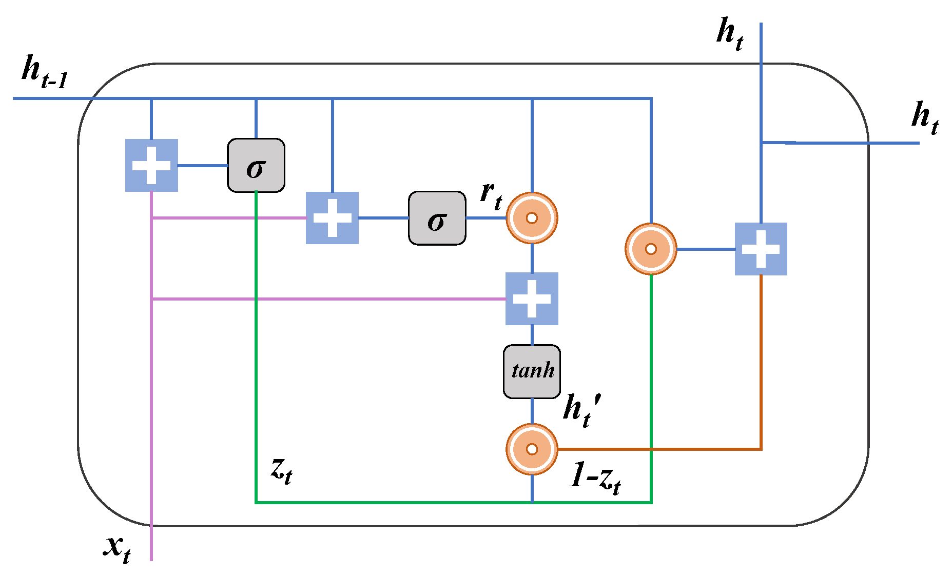
A GRU network, which is a variant of an RNN (Figure 1), can help resolve the long-term memory and gradient problems associated with backpropogation [45]. A GRU network can achieve an equivalent effect to that achieved by an LSTM network; however, training a GRU network is considerably easier than training an LSTM network, and the training efficiency of a GRU network is greater than that of an LSTM network. A GRU network contains two control gates: the reset and update gates. The calculation results of the hidden layer’s memory unit are not retained. The update gate directly controls the input and output, whereas the reset gate directly acts on the hidden-state gate control. The outputs of the reset gate $r$ and update gate $z$ are expressed as follows:

$$r_t=\sigma \left({\mathrm{W}}_r{x}_t+U_r{h}_{t-1}\right)$$

(17)

$$z_t=\sigma \left({\mathrm{W}}_z{x}_t+U_z{h}_{t-1}\right)$$

(18)

In a GRU model, the overlap between the current moment’s information and the historical information depends on the calculation process of the candidate hidden layer. The reset gate $r_t$ can obtain the output of the candidate hidden layer. When $r_t$ = 0, ${\tilde{h}}_t$ includes only the current input. The output of the candidate hidden layer is expressed as follows:

$${\tilde{h}}_t=\tan \mathrm{h}\left(W{x}_t+r_{t}U{h}_{t-1}\right)$$

(19)

When outputting the information of the hidden layer’s memory unit, the GRU model must control the percentage of information saved in the previous moment in the hidden layer and obtain the output by adding the information of the candidate hidden layer ${\tilde{h}}_t$. The output of the memory unit in the hidden layer is calculated as follows:

$$h_t=z_t\odot h_{t-1}+\left(1-z_t\right)\odot {\tilde{h}}_t$$

(20)

The output $z_t$ of the update gate affects the quantity of information that is calculated in the hidden layer at the current moment and retained by the hidden layer’s output $h_t$. When $z_t$ is close to 0, the information in the hidden layer can be regarded as abandoned information. When $z_t$ is close to 1, the information in the hidden layer can be directly copied to the current moment. This property of the update gate allows a GRU model to control the reliance of time sequence information on the step length and achieve the same learning capacity as an LSTM model for a time sequence.

3.4. Proposed Method

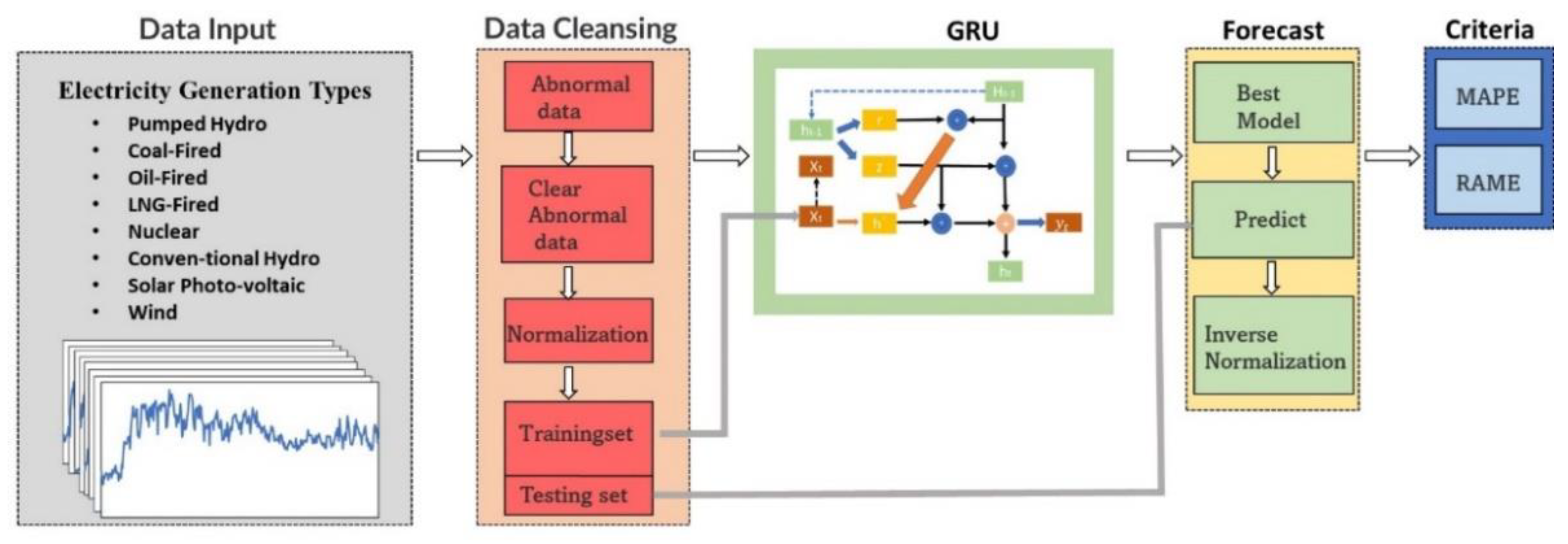
To construct a power generation prediction model applicable to Taiwan, data on the production of coal power, oil power, liquefied natural gas (LNG) power, conventional hydropower, solar photovoltaic power, wind power, pumped hydropower, and nuclear power in Taiwan were used as input data. Cleansing was required to detect abnormal data into the clear abnormal data for normalization and for splitting the training set and testing set into GRU neural network hyperparameters, which led how the network functioned and further determined its accuracy and validity. GRU hyperparameters must be adjusted appropriately to use GRU networks successfully in different domains. These hyperparameters include the number of hidden layers, number of neurons, learning rate, activation function, batch size, epoch, and loss function. In this study, the GRU hyperparameters were adjusted manually by the experts depending on how the hyperparameter values affected model performance. A learning rate of 0.0001 was adopted in this study. Rectified linear units (ReLUs) were used in all the activation functions because in addition to the simple calculation process, ReLUs can perform gradient descent and reverse transfer efficiently, thereby avoiding problems with exploding and vanishing gradients. The hyperparameters were adjusted to optimal values to achieve superior prediction results. The complete flowchart of power generation forecasting is displayed in Figure 2.

3.5. Performance Criteria

The performance of the developed prediction model was evaluated in terms of the root mean square error (RMSE), mean absolute percentage error (MAPE), and coefficient of determination (R²), which are expressed in Equations (21)–(23), respectively:

$$\mathrm{RMSE}=\sqrt{\frac{1}{N}{\displaystyle \sum _{i=1}^N{\left(y_i-f_i\right)}^2}}$$

(21)

$$\mathrm{MAPE}=\frac{1}{N}{\displaystyle \sum _{i=1}^N\left|\frac{y_i-f_i}{y_i}\right|}\times 100\%$$

(22)

$$\mathrm{R}2={\left[\frac{{{\displaystyle \sum }}_{i=1}^n\left({\eta }_{io}-{\overline{\eta }}_o\right)\left({\eta }_{iM}-{\overline{\eta }}_M\right)}{\sqrt{{{\displaystyle \sum }}_{i=1}^n{\left({\eta }_{io}-{\overline{\eta }}_o\right)}^2{{\displaystyle \sum }}_{i=1}^n{\left({\eta }_{iM}-{\overline{\eta }}_M\right)}^2}}\right]}^2$$

(23)

where $\eta$_io is the observed power generation in the ith time step, $\eta$_iM is the simulated power generation in the ith time step, n is the number of time steps, ${\overline{\eta }}_o$ is the mean of the observational values for power generation, and ${\overline{\eta }}_M$ is the mean of the simulated values for power generation.

4. Results

4.1. Data Sets

Data on Taiwan’s monthly electricity generation from 1991 to 2020 were obtained from the Energy Bureau of the Ministry of Economic Affairs in Taiwan. These data were divided into two subsets: the training set, which comprised monthly data from 1991 to 2016, and the testing set, which comprised monthly data from 2017 to 2020. The main types of power generation in Taiwan are thermal power (coal, oil, and LNG), renewable power (conventional hydropower, solar photovoltaic, and wind), pumped hydropower, and nuclear power (

Table 2. Electricity generation statistics for eight types of power generation in Taiwan from 1991 to 2020.

Data Set	SD (TWh)	Min (TWh)	Max (TWh)	Mean (TWh)	COV (%)
Coal-Fired	7.23	35.19	78.32	55.11	0.13
Oil-Fired	4.44	8.24	24.29	8.24	0.53
LNG-Fired	18.11	7.53	72.87	36.72	0.49
Conventional Hydro	1.56	1.44	10.56	3.57	0.43
Solar Photovoltaic	0.054	0	0.31	0.024	2.24
Wind	0.35	0	1.4	0.38	0.93
Pumped Hydro	0.35	2.24	3.74	2.83	0.12
Nuclear	5.59	10.83	39.24	31.1	0.17

SD, standard deviation; COV, coefficient of variation.

).

4.2. Energy Mix in Taiwan

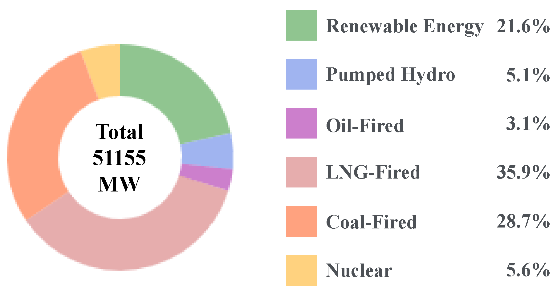
In 2021, 67.7%, 5.6%, and 21.6% of the power generated in Taiwan were from fossil fuel, nuclear, and renewable sources, respectively (Figure 3). The share of renewables in Taiwan’s energy mix has increased over time due to greater environmental consciousness among regulators and members of the public. However, the outputs of renewable power systems are unpredictable because they are highly dependent on weather. Therefore, the accurate prediction of the output of renewable energy systems is a challenge that must be overcome for renewable energy to be a viable part of the energy mix.

4.3. Parameter Settings

SVR has three hyperparameters: the penalty constant (C), insensitive loss function (ε), and bandwidth of the sum kernel function (σ). These parameters considerably affect the accuracy of SVR prediction, and poorly selected parameters result in overfitting or underfitting. The SVR model adopted in this study uses grid search (GS) to determine the best hyperparameters. GRID SVR adds the hyperparameters [46] in an exponential manner. In this study, the search parameters were set as follows: C = (2⁰~2¹⁰), ε = (2⁻⁸–2¹), and σ = (2⁻⁸–2¹).

Table 3. Training results obtained with support vector regression (SVR) and whale-optimization-algorithm-based SVR (WOASVR) under different parameter settings.

SVR				WOASVR
Data Set	C	ε	σ	C	ε	σ
Coal-Fired	16	0.0312	0.007812	36.10	0.704	0.003
Oil-Fired	8	0.0009	0.007812	17.43	0.033	0.003
LNG-Fired	32	0.0156	0.003906	282.3	0.003	0.003
Conventional Hydro	16	0.0009	0.00195	4.765	0.007	0.007
Solar Photovoltaic	4	0.0009	0.01562	1.007	0.003	0.003
Wind	1	0.0009	0.0625	198.6	0.146	0.003
Pumped Hydro	512	0.062	0.00097	1.209	0.057	0.004
Nuclear	4	0.062	0.01562	58.67	0.085	0.003

lists the training results obtained using the SVR and WOASVR models, including the hyperparameters selected for energy generation prediction. The results indicate that the WOA achieved superior hyperparametric optimization to the GS function.

4.4. Analysis of the Forecasting Results

Many studies have conducted energy forecasting, including power load forecasting for an energy management system [47], wind power supply forecasting for the Northeast Power Grid in Brazil [48], and renewable power demand forecasting for a smart grid and smart buildings [49].

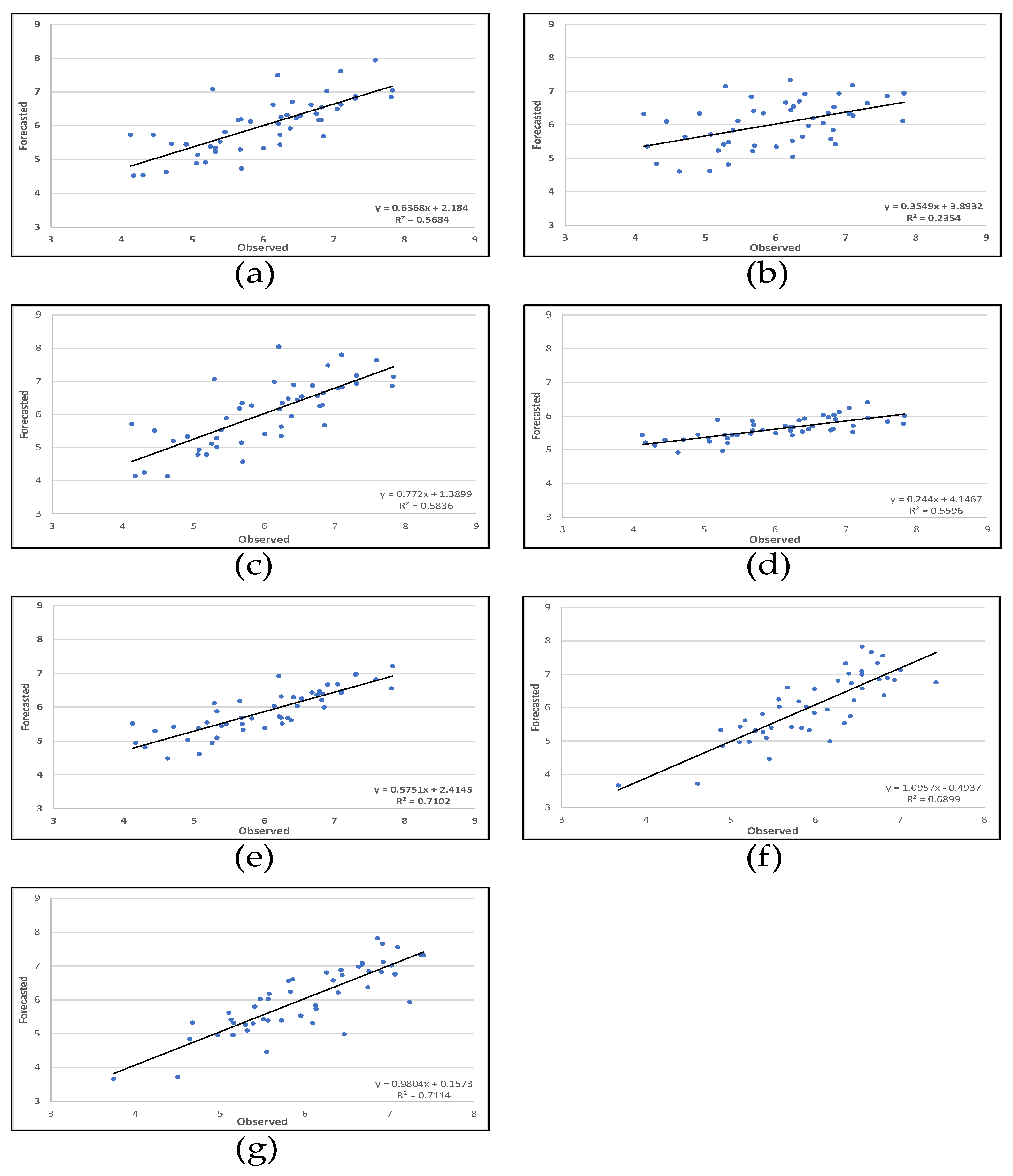
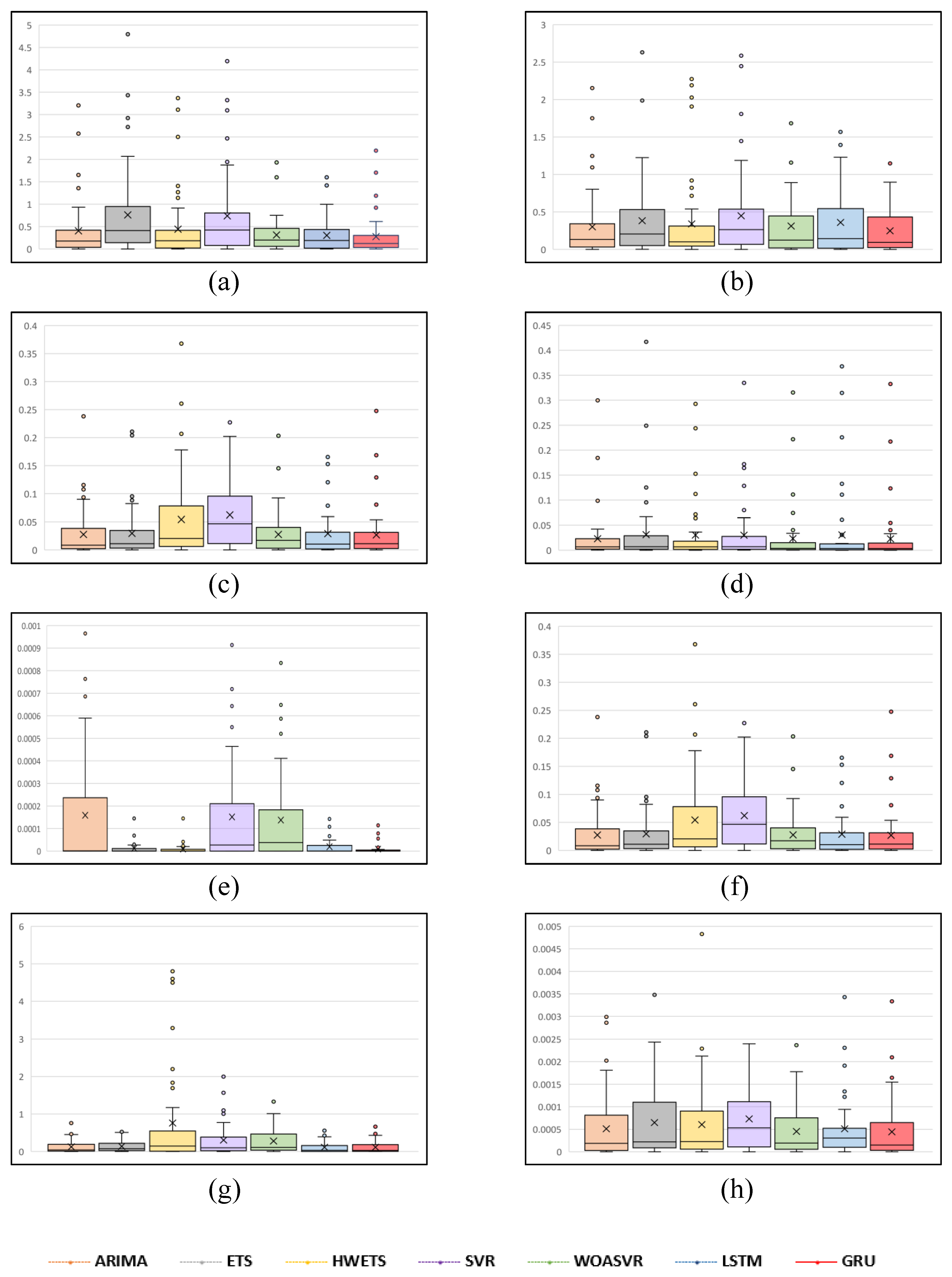
In this study, a GRU-based deep learning approach was developed to construct an accurate power-generation forecasting model. The power generation data for the first 48 months of the forecast were used to forecast the power-generation capacity. The developed deep learning approach is relatively unaffected by weather or other factors. The prediction performance of the developed GRU model was compared with that of three statistical models (the ARIMA, ETS, and HWETS models), two machine learning models (the SVR and WOASVR models), and one deep learning model (the LSTM model). MAPE and RMSE were used as criteria for examining model performance. The average values of these parameters for the aforementioned models are presented in

Table 4. Power generation predictions obtained using different methods for the period from 1 January 2018, to 31 December 2020.

Electricity Generation		Criteria	ARIMA	ETS	HWETSTS	SVR	WOA SVR	LSTM	GRU
Thermal Power	Coal-Fired	MAPE (%)	8.44	12.54	8.61	11.35	8.1	7.39	7.04
		RMSE	6.36	8.72	6.63	8.6	5.59	5.51	5.24
	LNG-Fired	MAPE (%)	7.22	8.58	7.47	9.04	7.28	7.94	6.69
		RMSE	5.5	6.19	5.83	6.69	5.59	6	4.98
	Oil-Fired	MAPE (%)	26.62	27.41	31.01	59.46	29.68	26.6	26.26
		RMSE	1.66	1.72	1.83	2.49	1.66	1.7	1.64
Renewable Energy	Conventional Hydro	MAPE (%)	30.39	33.62	28.38	33.49	25.63	24.86	24.26
		RMSE	1.51	1.76	1.74	1.72	1.52	1.74	1.5
	Solar Photovoltaic	MAPE (%)	50.41	21.7	17.53	52.87	50.57	21.36	17.4
		RMSE	0.12	0.041	0.03	0.12	0.11	0.44	0.02
	Wind	MAPE (%)	60.39	50.94	36.12	69.9	37.28	35.68	31.98
		RMSE	0.45	0.32	0.25	0.33	0.27	0.26	0.18
Nuclear		MAPE (%)	13.32	14.27	29.44	55.37	17.77	13.60	13.25
		RMSE	3.54	3.71	8.71	15.55	5.27	3.39	3.37
Pumped Hydro		MAPE (%)	6.35	7.4	7.02	8.92	6.31	6.68	6.13
		RMSE	0.22	0.25	0.24	0.27	0.21	0.22	0.21
Average		MAPE (%)	25.77	22.05	20.69	37.55	21.82	18.01	16.62
		RMSE	2.37	2.83	3.15	4.47	2.52	2.4	2.14

MAPE, mean absolute percentage error; RMSE, root mean square error; boldface, the optimal values in each row. ARIMA, autoregressive composite moving average; ETS, exponential smoothing; HWETS, holt winters exponential smoothing; SVR, which supports vector regression; WOASVR, whale optimization algorithm-based support vector regression; LSTMs, long short-term memory; GRU, gated recurrent unit.

. The HWETS, SVR, WOASVR, and LSTM models by 9.15%, 5.43%, 4.07%, 20.93%, 5.2%, and 1.39% RMSE values were lower than those of ARIMA, ETS, HWETS, SVR, WOASVR, and LSTM models by 1.2%, 3.5%, 5.1%, 11.7%, and 1.9%. The aforementioned results indicate the considerably greater predictive accuracy of the WOASVR model relative to the ARIMA, ETS, HWETS, SVR, WOASVR, and LSTM models (Figure 4).

Figure 5 shows the actual and predicted power generation values generated by ARIMA, ETS, HWETS, SVR, WOASVR, LSTM, and GRU models in the prediction process. The figure shows that the prediction results of the GRU model and the other statistical models are more concentrated. The GRU model shows the best prediction results, and its scatter distribution is the closest to the regression line.

5. Discussion

5.1. ETS, ARIMA, and HWETS Models

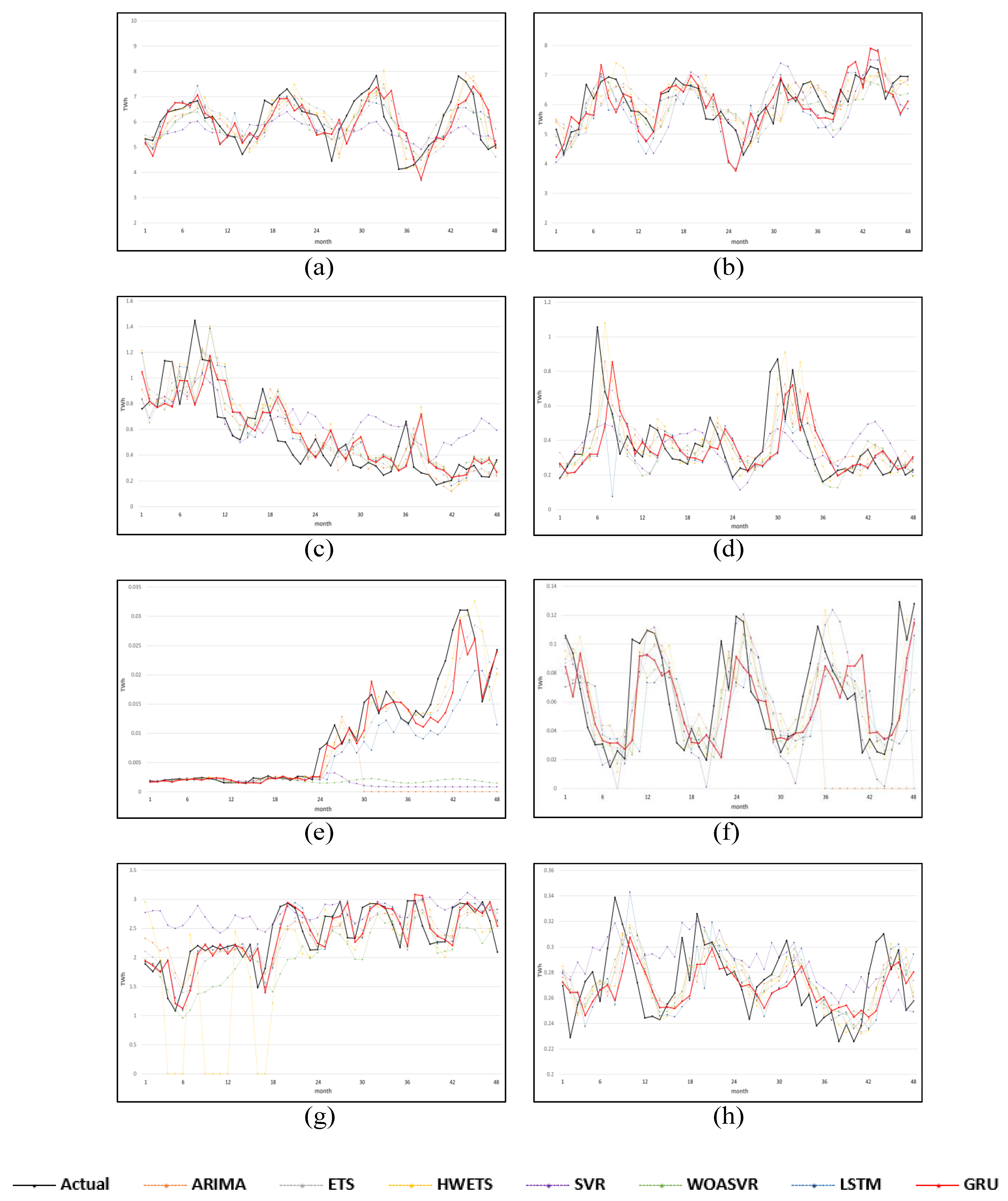
Large historical data sets are required to determine the optimal parameter combination for the ARIMA model. HWETS is used to model three aspects of time series: average, trend, and seasonality. The HWETS model predicts current or future values according to the comprehensive effects of these three aspects; thus, this model is suitable for nonstationary series containing linear trends and periodic fluctuation. However, the HWETS model is computationally expensive. In general, nonlinear problems cannot be easily solved using statistical models such as ETS, HWETS, and ARIMA. As displayed in Figure 5 and Figure 6, the HWETS models consistently had the highest error among the compared models. Figure 5e shows that the prediction accuracy of ARIMA is quite low. This may be attributed to the fact that the historical solar photovoltaic power generation is quite small; however, due to the impact of Taiwan’s energy policy, the solar power generation in 2020 increased significantly, resulting in a significant inaccuracy in the prediction of ARIMA model.

5.2. Comparison between SVR and WOASVR Models

Hybrid machine learning methods tend to be more accurate than any single machine learning method. For example, in the WOASVR algorithm, particle swarm optimization (PSO) is used to overcome the drawbacks of the SVR. PSO, which was proposed in 1995 by Eberhart and Kennedy, is a population-based optimization algorithm inspired by the foraging behavior of bird flocking. The SVR has three hyperparameters, namely, the regularization parameter (C), bandwidth of the kernel function (σ), and ε-insensitive loss function (ε), and variations in these hyperparameters considerably affect the forecasting accuracy of SVR. The automatic adjustment of these three hyperparameters remains a formidable challenge in improving the forecasting accuracy of SVR. PSO can be used to optimize the hyperparameters of the SVR algorithm to prevent overfitting or underfitting [38]. Because the hyperparameters are optimized in WOASVR, the WOASVR model exhibited lower MAPE and RMSE than did the the SVR model (Figure 5 and Figure 6). A special case can be found in Figure 5e: the prediction of SVR and WOASVR is quite poor. The inference is that as the hyperparameters are not adjusted to the best and are affected by the trend of historical data, the model training is poor. Therefore, it is impossible to simulate the curve when the power generation increases.

5.3. Comparison between the LSTM and GRU Models

Since 2015, deep learning has gained substantial popularity in the machine learning community because it provides a general framework for training deep neural networks with many hidden layers [50]. Deep learning has been widely used to solve several types of time-series forecasting problems. Of these models, RNNs have received considerable attention because they have short-term memory on account of recurrent feedback connections; thus, RNN is suitable for modeling time-series data [51,52].

An LSTM network, which is a time-recurrent neural network, is another suitable deep learning network for solving time-series problems. An LSTM network has long-term memory and overcomes most of the drawbacks of RNNs; however, in practice, LSTM networks require a long training time. The total number of gates in a GRU network is half that in an LSTM network; thus, GRU networks are simpler variants of LSTM networks and are widely used in various applications. A GRU network can be almost as accurate as an LSTM network but with a shorter training time. Figure 6 indicates that in power generation prediction, the error of the developed GRU model was lower than that of the LSTM model. The error of the GRU model was marginally higher than that of the LSTM model only for the predictions of the pumped hydropower generation. Table 4 shows that the prediction results of GRU in thermal power are not significantly different from those of other models, but the prediction of renewable energy is quite prominent. As the statistical model infers the prediction value from historical data to a great extent, it is difficult to make an effective prediction of nonlinear answers. The deep learning model showed a stronger prediction ability and a better extraction ability of abstract features through neuron and activation function. The research results also showed that the average MAPE of GRU was lower than that of other models.

5.4. Effect of CO₂ Emissions

Countries have increasingly recognized the urgent need for emission reductions in the fight against climate change, especially in the wake of 2015 Paris Agreement and 2005 Kyoto Protocol, and technology has become a means toward that end [53].

Mechanisms have been established across the globe to reduce CO₂ emissions in the power sector at the supply side (e.g., increasing the share of renewable energy and nuclear energy in the energy mix and implementing carbon capture and storage technologies) and demand side (e.g., promoting electricity-saving measures and the use of efficient appliances). For example, authorities in the United States have formulated policies mandating (i) the abolition of subsidies for traditional electricity technologies, (ii) the accurate pricing of electricity by usage, (iii) the introduction of nationwide feed-in-tariff scheme, and (iv) the creation of a national fund for public awareness. The authors of [54,55] found that CO₂ emissions in Europe can be decreased to appropriate levels by using technologies running on renewable energy, making wind the dominant power source, and adopting high-efficiency measures. The share of solar energy in the global energy supply mix might exceed 10% by 2050; however, this share of renewable energy supply would provide little help in achieving the required reduction (i.e., up to 75%) in the carbon intensity of the power generation worldwide [56]. The intermittent nature of renewable resources adds to the difficulty of using them as the sole sources for electricity supply in the world.

According to the National Electricity Supply and Demand Report, 98% of Taiwan’s energy is imported. Energy prices and supply are volatile because they are deeply intertwined with geopolitics. In addition, Taiwan’s power system is connected to an independent power grid and cannot receive foreign assistance should power supply be insufficient, which would lead to social unrest, national insecurity, and economic disruption. Therefore, Taiwan’s energy mix must be diversified for its energy security to be ensured. In 2016, the Taiwanese government amended the Electricity Act, established an energy transformation policy, and stipulated that the operation of all nuclear power generation equipment must cease by 2025. Based on this, the overall goal of Taiwan’s energy transformation has been zeroed in and practically reviewed. The current policy is compliant with the provisions of the referendum law. Therefore, under the conditions of ensuring power supply stability and implementing relevant supporting measures, the goal of national energy transformation can be achieved in Taiwan.

6. Conclusions

Energy is scarce. Thus, it is mandatory that societies reduce energy wastage and ensure stable power supply to avoid the lack of power rationing that affects industrial economic development and people’s livelihoods. To avoid major losses, long-term power generation supply planning, should try to grasp the future of the annual power generation demand. Renewables will occupy a much larger share in Taiwan’s energy mix, but renewable power generation is unpredictable due to its susceptibility to changes in weather. Thus, this study developed a GRU model that accurately predicts the level of power generation from renewables in Taiwan. In evaluation experiments, this model outperformed three statistical models (the ARIMA, ETS, and HWETS models), two machine learning models (the SVR and WOASVR models), and one deep learning model (the LSTM model) with respect to accuracy.

References

- United Nations. United Nations Energy Mechanism; United Nations: New York, NY, USA, 2022. [Google Scholar]
- United Nations. United Nations Sustainable Development Goals; United Nations: New York, NY, USA, 2015. [Google Scholar]
- Bureau of Energy, Ministry of Economic Affairs. Energy Statistics Handbook 2020; ROC: Taipei City, Taiwan, 2020. [Google Scholar]
- Yuan, E. Sustainable Energy Policy Framework; ROC: Taipei City, Taiwan, 2008. [Google Scholar]
- Bureau of Energy, Ministry of Economic Affairs. 108_109 National Electricity Supply and Demand Report; ROC: Taipei City, Taiwan, 2019. [Google Scholar]
- Hou, C.; Wu, J.; Cao, B.; Fan, J. A deep-learning prediction model for imbalanced time series data forecasting. Big Data Min. Anal. 2021, 4, 266–278. [Google Scholar] [CrossRef]
- Amini, M.; Karabasoglu, O.; Ilić, M.D.; Boroojeni, K.G.; Iyengar, S. Arima-based demand forecasting method considering probabilistic model of electric vehicles’ parking lots. In Proceedings of the 2015 IEEE Power & Energy Society General Meeting, Denver, CO, USA, 26–30 July 2015; pp. 1–5. [Google Scholar]
- Xydas, S.; Marmaras, C.; Cipcigan, L.M.; Hassan, A.; Jenkins, N. Electric vehicle load forecasting using data mining methods. In Proceedings of the IET Hybrid and Electric Vehicles Conference 2013 (HEVC 2013), London, UK, 6–7 November 2013. [Google Scholar]
- Xiaobo, X.; Liu, W.; Xi, Z.; Tianyang, Z. Short-term load forecasting for the electric bus station based on GRA-DE-SVR. In Proceedings of the 2014 IEEE Innovative Smart Grid Technologies-Asia (ISGT ASIA), Kuala Lumpur, Malaysia, 20–23 May 2014; pp. 388–393. [Google Scholar]
- Kotillová, A. Very short-term load forecasting using exponential smoothing and ARIMA models. J. Inf. Control Manag. Syst. 2011, 9, 85–92. [Google Scholar]
- Tan, B.; Ma, X.; Shi, Q.; Guo, M.; Zhao, H.; Shen, X. Ultra-short-term Wind Power Forecasting Based on Improved LSTM. In Proceedings of the 2021 6th International Conference on Power and Renewable Energy (ICPRE), Shanghai, China, 17–20 November 2021; pp. 1029–1033. [Google Scholar]
- Li, W.; Shi, Q.; Sibtain, M.; Li, D.; Mbanze, D.E. A hybrid forecasting model for short-term power load based on sample entropy, two-phase decomposition and whale algorithm optimized support vector regression. IEEE Access 2020, 8, 166907–166921. [Google Scholar] [CrossRef]
- Saini, V.K.; Bhardwaj, B.; Gupta, V.; Kumar, R.; Mathur, A. Gated Recurrent Unit (GRU) Based Short Term Forecasting for Wind Energy Estimation. In Proceedings of the 2020 International Conference on Power, Energy, Control and Transmission Systems (ICPECTS), Chennai, India, 10–11 December 2020; pp. 1–6. [Google Scholar]
- Sreekumar, S.; Sharma, K.; Bhakar, R.; Chawda, S.; Teotia, F.; Prakash, V. Deviation Charge Reduction of Aggregated Wind Power Generation using Intelligently Tuned Support Vector Regression. In Proceedings of the 2019 8th International Conference on Power Systems (ICPS), Jaipur, India, 20–22 December 2019; pp. 1–6. [Google Scholar]
- Xinyun, L.; Huidan, L.; Hang, Y.; Zilan, C.; Bangdi, C.; Yi, Y. IoT Data Acquisition Node For Deep Learning Time Series Prediction. In Proceedings of the 2021 2nd International Conference on Big Data Analytics and Practices (IBDAP), Bangkok, Thailand, 26–27 August 2021; pp. 107–111. [Google Scholar]
- Kumar, S.; Hussain, L.; Banarjee, S.; Reza, M. Energy load forecasting using deep learning approach-LSTM and GRU in spark cluster. In Proceedings of the 2018 Fifth International Conference on Emerging Applications of Information Technology (EAIT), Kolkata, India, 12–13 January 2018; pp. 1–4. [Google Scholar]
- Yatiyana, E.; Rajakaruna, S.; Ghosh, A. Wind speed and direction forecasting for wind power generation using ARIMA model. In Proceedings of the 2017 Australasian Universities Power Engineering Conference (AUPEC), Melbourne, Australia, 19–22 November 2017; pp. 1–6. [Google Scholar]
- Wei, L.; Zhen-gang, Z. Based on time sequence of ARIMA model in the application of short-term electricity load forecasting. In Proceedings of the 2009 International Conference on Research Challenges in Computer Science, Shanghai, China, 28–29 December 2009; pp. 11–14. [Google Scholar]
- Peng, B.; Liu, L.; Wang, Y. Monthly electricity consumption forecast of the park based on hybrid forecasting method. In Proceedings of the 2021 China International Conference on Electricity Distribution (CICED), Shanghai, China, 7–9 April 2021; pp. 789–793. [Google Scholar]
- Panigrahi, S.; Behera, H.S. A hybrid ETS–ANN model for time series forecasting. Eng. Appl. Artif. Intell. 2017, 66, 49–59. [Google Scholar] [CrossRef]
- Alam, T.; AlArjani, A. Forecasting CO2 Emissions in Saudi Arabia Using Artificial Neural Network, Holt-Winters Exponential Smoothing, and Autoregressive Integrated Moving Average Models. In Proceedings of the 2021 International Conference on Technology and Policy in Energy and Electric Power (ICT-PEP), Yogyakarta, Indonesia, 29–30 September 2021; pp. 125–129. [Google Scholar]
- Nambiar, M.L.; Geethalekshmy, V.; Mohan, A. Forecasting Solar Energy Generation and Load Consumption-A Method to select the forecasting model based on data type. In Proceedings of the 2019 2nd International Conference on Intelligent Computing, Instrumentation and Control Technologies (ICICICT), Kerala, India, 5–6 July 2019; pp. 1491–1495. [Google Scholar]
- Elattar, E.E.; Goulermas, J.; Wu, Q.H. Electric load forecasting based on locally weighted support vector regression. IEEE Trans. Syst. Man Cybern. Part C Appl. Rev. 2010, 40, 438–447. [Google Scholar] [CrossRef]
- Osama, S.; Darwish, A.; Houssein, E.H.; Hassanien, A.E.; Fahmy, A.A.; Mahrous, A. Long-Term Wind Speed Prediction based on Optimized Support Vector Regression. In Proceedings of the 2017 Eighth International Conference on Intelligent Computing and Information Systems (ICICIS), Cairo, Egypt, 5–7 December 2017; pp. 191–196. [Google Scholar]
- Fu, Y.; Hu, W.; Tang, M.; Yu, R.; Liu, B. Multi-Step Ahead Wind Power Forecasting based on Recurrent Neural Networks. In Proceedings of the 2018 IEEE PES Asia-Pacific Power and Energy Engineering Conference (APPEEC), Sabah, Malaysia, 7–10 October 2018; pp. 217–222. [Google Scholar]
- Li, J.; Geng, D.; Zhang, P.; Meng, X.; Liang, Z.; Fan, G. Ultra-Short Term Wind Power Forecasting based on LSTM Neural Network. In Proceedings of the 2019 IEEE 3rd International Electrical and Energy Conference (CIEEC), Beijing, China, 7–9 September 2019; pp. 1815–1818. [Google Scholar]
- Rajagukguk, R.A.; Ramadhan, R.A.; Lee, H.-J. A review on deep learning models for forecasting time series data of solar irradiance and photovoltaic power. Energies 2020, 13, 6623. [Google Scholar] [CrossRef]
- Nguyen, T.-A.; Pham, M.-H.; Duong, T.-K.; Vu, M.-P. A Recent Invasion Wave Of Deep Learning In Solar Power Forecasting Techniques Using Ann. In Proceedings of the 2021 IEEE International Future Energy Electronics Conference (IFEEC), Taipei, Taiwan, 16–19 November 2021; pp. 1–6. [Google Scholar]
- Box, G.E.; Jenkins, G.M. Time series analysis: Forecasting and control. Oper. Res. Q. 1976, 22, 199–201. [Google Scholar]
- Kreuzer, D.; Munz, M.; Schlüter, S. Short-term temperature forecasts using a convolutional neural network—An application to different weather stations in Germany. Mach. Learn. Appl. 2020, 2, 100007. [Google Scholar] [CrossRef]
- Brown, R.G.; Meyer, R.F. The fundamental theorem of exponential smoothing. Oper. Res. 1961, 9, 673–685. [Google Scholar] [CrossRef]
- Hyndman, R.; Koehler, A.B.; Ord, J.K.; Snyder, R.D. Forecasting with Exponential Smoothing: The State Space Approach; Springer Science & Business Media: Berlin/Heidelberg, Germany, 2008. [Google Scholar]
- Hyndman, R.J.; Khandakar, Y. Automatic time series forecasting: The forecast package for R. J. Stat. Softw. 2008, 27, 1–22. [Google Scholar] [CrossRef] [Green Version]
- Winters, P.R. Forecasting sales by exponentially weighted moving averages. Manag. Sci. 1960, 6, 324–342. [Google Scholar] [CrossRef]
- Supranto, J. Statistics: Theory and Applications, 6th ed.; Erlangga: Jakarta, Indonesia, 2000. [Google Scholar]
- Vapnik, V.; Golowich, S.E.; Smola, A.J. Support vector method for function approximation, regression estimation and signal processing. In Proceedings of the Advances in Neural Information Processing Systems, Denver, CO, USA, 2–5 December 1996; pp. 281–287. [Google Scholar]
- Mirjalili, S.; Lewis, A. The whale optimization algorithm. Adv. Eng. Softw. 2016, 95, 51–67. [Google Scholar] [CrossRef]
- Liu, H.-H.; Chang, L.-C.; Li, C.-W.; Yang, C.-H. Particle swarm optimization-based support vector regression for tourist arrivals forecasting. Comput. Intell. Neurosci. 2018, 2018, 6076475. [Google Scholar] [CrossRef]
- Yang, S.; Chen, H.-C.; Chen, W.-C.; Yang, C.-H. Student Enrollment and Teacher Statistics Forecasting Based on Time-Series Analysis. Comput. Intell. Neurosci. 2020, 2020, 1246920. [Google Scholar] [CrossRef]
- Yang, C.-H.; Wu, C.-H.; Hsieh, C.-M.; Wang, Y.-C.; Tsen, I.-F.; Tseng, S.-H. Deep Learning for Imputation and Forecasting Tidal Level. IEEE J. Ocean. Eng. 2021, 46, 1261–1271. [Google Scholar] [CrossRef]
- Abdel-Nasser, M.; Mahmoud, K. Accurate photovoltaic power forecasting models using deep LSTM-RNN. Neural Comput. Appl. 2019, 31, 2727–2740. [Google Scholar] [CrossRef]
- Wu, W.; Liao, W.; Miao, J.; Du, G. Using gated recurrent unit network to forecast short-term load considering impact of electricity price. Energy Procedia 2019, 158, 3369–3374. [Google Scholar] [CrossRef]
- Rumelhart, D.E.; Hinton, G.E.; Williams, R.J. Learning representations by back-propagating errors. Nature 1986, 323, 533–536. [Google Scholar] [CrossRef]
- Hochreiter, S.; Schmidhuber, J. Long short-term memory. Neural Comput. 1997, 9, 1735–1780. [Google Scholar] [CrossRef]
- Cho, K.; Van Merriënboer, B.; Bahdanau, D.; Bengio, Y. On the properties of neural machine translation: Encoder-decoder approaches. arXiv 2014, arXiv:1409.1259. [Google Scholar]
- Wauters, M.; Vanhoucke, M. Support vector machine regression for project control forecasting. Autom. Constr. 2014, 47, 92–106. [Google Scholar] [CrossRef] [Green Version]
- Ahmad, T.; Chen, H. Nonlinear autoregressive and random forest approaches to forecasting electricity load for utility energy management systems. Sustain. Cities Soc. 2019, 45, 460–473. [Google Scholar] [CrossRef]
- de Jong, P.; Dargaville, R.; Silver, J.; Utembe, S.; Kiperstok, A.; Torres, E.A. Forecasting high proportions of wind energy supplying the Brazilian Northeast electricity grid. Appl. Energy 2017, 195, 538–555. [Google Scholar] [CrossRef]
- Ahmad, T.; Zhang, H.; Yan, B. A review on renewable energy and electricity requirement forecasting models for smart grid and buildings. Sustain. Cities Soc. 2020, 55, 102052. [Google Scholar] [CrossRef]
- Schmidhuber, J. Deep learning in neural networks: An overview. Neural Netw. 2015, 61, 85–117. [Google Scholar] [CrossRef] [Green Version]
- Sagheer, A.; Kotb, M. Time series forecasting of petroleum production using deep LSTM recurrent networks. Neurocomputing 2019, 323, 203–213. [Google Scholar] [CrossRef]
- Tealab, A. Time series forecasting using artificial neural networks methodologies: A systematic review. Future Comput. Inform. J. 2018, 3, 334–340. [Google Scholar] [CrossRef]
- Mengal, A.; Mirjat, N.H.; Walasai, G.D.; Khatri, S.A.; Harijan, K.; Uqaili, M.A. Modeling of future electricity generation and emissions assessment for Pakistan. Processes 2019, 7, 212. [Google Scholar] [CrossRef] [Green Version]
- Sovacool, B.K. The importance of comprehensiveness in renewable electricity and energy-efficiency policy. Energy Policy 2009, 37, 1529–1541. [Google Scholar] [CrossRef]
- Foerster, H.; Healy, S.; Loreck, C.; Matthes, F.; Fischedick, M.; Lechtenboehmer, S.; Samadi, S.; Venjakob, J. Information for Policy Makers 2. Analysis of the EU’s Energy Roadmap 2050 Scenarios; SEFEP—Smart Energy for Europe Platform GmbH: Berlin, Germany, 2012. [Google Scholar]
- Timilsina, G.R.; Kurdgelashvili, L.; Narbel, P.A. Solar energy: Markets, economics and policies. Renew. Sustain. Energy Rev. 2012, 16, 449–465. [Google Scholar] [CrossRef]
Figure 1.
The architecture of a gated recurrent unit (GRU).
Figure 2.
Flow chart of electricity demand forecasting.
Figure 3.
Energy mix in Taiwan in 2021.
Figure 4.
Scatter plots of the predictions obtained for coal energy generation (48−month forecasts) for the period from 1 January 2017, to 31 December 2020, when different methods were used: (a) autoregressive composite moving average (ARIMA), (b) exponential smoothing (ETS), (c) Holt−Winters ETS (HWETS), (d) SVR, (e) WOASVR, (f) long short-term memory (LSTM), and (g) GRU.
Figure 5.
Predictions obtained using the seven models for (a) the generation of coal power, (b) liquefied natural gas (LNG) power, (c) oil power, (d) conventional hydropower, (e) solar photovoltaic power, (f) wind power, (g) nuclear power, and (h) pumped hydropower.
Figure 6.
Scatter plots of power generation forecasts (48-month forecasts) for the period from 1 January 2017 to 31 December 2020, when different methods were used: forecasts of (a) coal power, (b) LNG power, (c) oil power, (d) conventional hydropower, (e) solar photovoltaic power, (f) wind power, (g) nuclear power, and (h) pumped hydropower.