An Efficient Method for Breast Mass Classification Using Pre-Trained Deep Convolutional Networks

Abstract

Masses are the early indicators of breast cancer, and distinguishing between benign and malignant masses is a challenging problem. Many machine learning- and deep learning-based methods have been proposed to distinguish benign masses from malignant ones on mammograms. However, their performance is not satisfactory. Though deep learning has been shown to be effective in a variety of applications, it is challenging to apply it for mass classification since it requires a large dataset for training and the number of available annotated mammograms is limited. A common approach to overcome this issue is to employ a pre-trained model and fine-tune it on mammograms. Though this works well, it still involves fine-tuning a huge number of learnable parameters with a small number of annotated mammograms. To tackle the small set problem in the training or fine-tuning of CNN models, we introduce a new method, which uses a pre-trained CNN without any modifications as an end-to-end model for mass classification, without fine-tuning the learnable parameters. The training phase only identifies the neurons in the classification layer, which yield higher activation for each class, and later on uses the activation of these neurons to classify an unknown mass ROI. We evaluated the proposed approach using different CNN models on the public domain benchmark datasets, such as DDSM and INbreast. The results show that it outperforms the state-of-the-art deep learning-based methods.

1. Introduction

Breast cancer is considered to be one of the most fatal diseases around the world that affects women, and according to the available data it causes around 25% more deaths than other cancers [1]. However, treatment at the early stages can reduce the risk of death. Otherwise, if it is not discovered at an early stage, the probability of death becomes very high [2]. Therefore, a computer-aided system is needed to save patients’ lives. In this regard, we have implemented a new computer-aided system to detect breast cancer and to classify mammogram images as benign or malignant. Much research has been conducted on this problem, and some studies have yielded good results [3,4,5,6,7]. Previous studies have either used hand-engineered feature representation [8,9,10] or a deep learning approach [3,4,5,6,7]. For the hand-crafted approach, the main limitations are its time-consuming nature and its need for an expert to determine what the suitable feature for a certain problem is [11]. For the deep learning approach, some deep learning-based methods design and train models from scratch [3,5,6,12,13,14], while others use pre-trained models and fine-tune them [4,7,11,15,16,17].

Though deep learning has exhibited excellent performance in many applications, it is challenging to apply it to breast cancer detection because it needs a huge dataset for training, but the number of available annotated data is limited [14]. In the case of medical images, especially for the problem of the classification of benign and malignant masses, we do not have a huge number of annotated data. There are two common approaches to overcome this issue: The first method is based on transfer learning. In this approach, the deep CNN model is first trained using a dataset with a massive number of images from a related domain such as ImageNet. Then, it is transferred and fine-tuned using a different dataset (mass ROIs of mammogram images in our case). The use of this approach requires a trained number of learnable parameters as the last fully connected layer is removed and a new layer is added. As mentioned earlier, if the amount of data is not enough, it causes the problem of over-fitting [9,14,18]. The second method is based on data augmentation by generating new training data. However, the main disadvantage of generating new data is the chance of losing the label-preserving property [15]. Thus, when generating new data, we need to monitor the newly produced data to make sure they have not transformed the label of the new image and to guarantee that the new samples are correctly generated and labeled [8]. Otherwise, there is a chance that wrong learning may occur, in which case data augmentation methods will cause a reduction or drop in the model performance. This leads to an increase in the misclassification risk. Moreover, data augmentation increases the computational time and cost [15].

To address the aforementioned issues, we propose a method for classifying mass ROIs as benign or malignant that uses a pre-trained CNN without any modification (such as removing the final fully connected layers, as is commonly done in all current cases) and thus eliminates the need for CNN model retraining or fine-tuning, as well as data augmentation. The proposed method does not require considerable parameter learning to train and fine-tune. Additionally, a large number of training data is not required to train the deep CNN model. We consider only the labels of the ROIs during the training phase rather than tuning or updating the learnable weights. The model detects the neurons in the final fully linked layer that are activated more strongly for each class and then utilizes their activation to identify an unknown mass’s ROI.

In comparison to prior works, the proposed method successfully produces state-of-the-art results. The main contributions of this research paper are:

• We show how to use a CNN model that has already been trained without modifying or fine-tuning it. We propose algorithms for the training and testing phases towards this aim. We propose a new simple mass classification method based on a pre-trained CNN model that does not necessitate a huge training dataset or fine-tuning of the learnable parameters in the same way that existing methods do. Only the neurons in the classification layer that have a higher degree of activity for each class are identified during the training phase. The neurons allocated to each are used to categorize unknown mass ROIs during the testing phase.
• We empirically examine the method using many well-known pre-trained CNN models, such as VGG16, VGG19, ResNet-50, ResNet-101, ResNet-18, DensNet, and GoogleNet, to identify which model performs the best.
• The proposed method is evaluated using the standard 10-fold CV and evaluation metrics such as precision, sensitivity, specificity, and F1-Score and is tested on two benchmark datasets (DDSM and INbreast).

This paper’s structure is as follows: The related literature is presented in Section 2. Section 3 describes the proposed method. In Section 4, we discuss the results of several experiments, and in Section 5 we present the conclusion and future work.

2. Literature Review

Many methods have been proposed to address this problem, which can be broadly categorized into hand-engineered-based methods and deep learning-based methods. In the following paragraphs, we give an overview of the state-of-the-art methods.

2.1. Hand-Engineering Approach

Chen et al. [12] applied a quantitative image analysis scheme to classify breast cancer mammography into benign and malignant. They extracted 59 spatial and frequency domain features, such as shape, density, block-based fast Fourier transform (FFT) features, discrete cosine transform (DCT) features, and wavelet transform (WT) features, from two views (CC and MLO) of the right and left sides. Then, they applied particle swarm optimization (PSO) to select discriminative features. They used the support vector machine (SVM) for classification. They validated the method using a full-field digital mammography (FFDM) dataset. Das et al. [9] proposed a new method of classifying mammography masses as benign or malignant. The input image is preprocessed using power-law transformations, and suspected regions are segmented to categorize masses. Morphological feature analysis and shift-invariant extrema characterization are applied to analyze the morphological mass spectrum for the segmented mass. ANN is used to classify masses as benign or malignant. Nagarajan et al. [16] decomposed the ROI using bi-dimensional empirical mode decomposition (BEMD) and modified bidimensional empirical mode decomposition (MBEMD). The features are then extracted using GLCM and gray level run length matrix (GLRM). Support vector machine (SVM) and linear discriminant analysis (LDA) classifiers are used to classify the input ROI masses as benign or malignant. They validated the method using MIAS, DDSM, and private datasets. Reenadevi, R. et al. [3] developed a CAD system to classify ROI images as normal, benign, or malignant. They used various statistical features and optimized the wrapper-based chaotic crow search algorithm (WCCSA) to select the most discriminative features and used a probabilistic neural network (PNN) for classification. The proposed method was evaluated using the mini-mamographic image analysis society (MIAS) dataset. Singh et al. [4] conducted research on the analysis of different textures and geometric feature extraction, feature selection, and classification of breast mass. The proposed system was tested using the INbreast dataset. They found that the Relief-F algorithm outperformed other feature selection algorithms, and the best result among the classifiers was given by K-NN. Shen et al. [10] proposed a CAD system for mammogram image classification into two classes: normal and abnormal. They enhanced mammography images using noise reduction and that further used image segmentation and morphological operations. They combined two hand-crafted features: discrete wavelet decomposition and GLCM. A deep belief network (DBN) is adopted for the classification. The system was tested using MIAS.

2.2. Deep Learning Approaches

2.2.1. Custom/New CNN Model/Architecture

Saira Charan et al. [8] built a CAD system for breast mass classification as normal or abnormal. Preprocessing, including morphological operations, connected component (CC) extraction, selection of the CC with the largest area, and masking, is used to remove noise and to extract the breast region only. They built a new convolutional neural network and trained it end-to-end using the MIAS dataset. Shakeel et al. [5] proposed a new CAD system to detect and classify masses as benign or malignant. They applied a region-based segmentation technique to extract ROIs and used contrast limited adaptive histogram equalization (CLAHE) to enhance the quality of the mammogram images. They designed a customized deep CNN model to extract the features. A support vector machine was used as a classifier. The DDSM dataset was used to train and evaluate the model. El Houby et al. [6] built their own CNN architecture to classify breast lesions as malignant or benign. They also applied the CLAHE algorithm for image enhancement. The model was evaluated using the INbreast, MIAS, and DDSM datasets.

2.2.2. Fine-Tuned Model

Sun et al. [13] proposed a multi-view and multi-dilated CNN model to incorporate complementary information from two views (MLO and CC) and a larger field of view for mass classification. They used LeNet as the backbone CNN model. They also modified cross-entropy loss function by adding the penalty term to enhance the classification accuracy. They validated the method using Digital Database for Screening Mammography (DDSM) and Mammographic Image Analysis Society (MIAS) datasets. Li et al. [17] proposed a new DenseNet model called DenseNet-II. They first performed the preprocessing phase to avoid overfitting caused by the small number of training data. Then, they enhanced the existing DenseNet CNN structure by replacing the first convolutional layer, the first layer before the first DenseBlock Layer, with an inception layer, which replaces the first 3 × 3 convolution in the DenseNet network. Finally, the preprocessing mammogram images were input into five CNN models (AlexNet, VGGNet, GoogleNet, DenseNet network model, and DenseNet-II). Ahmed et al. [7] implemented a new technique to detect and classify tumors in breast mammography images. They used preprocessing methods such as noise removal, morphological operation, and contrast limited adaptive histogram equalization (CLAHE) to enhance the image quality. Segmentation and augmentation were applied to reduce the processing time. They applied transfer learning with pre-trained VGGs (VGG16 & VGG19) as the backbone network for feature extraction. The last step used softMax to classify the images into three classes: normal, benign, or malignant. The model was fine-tuned and tested using the INbreast dataset. Sannasi et al. [19] studied the performance of different CNN architectures for the breast cancer classification problem. They performed many experiments using pre-trained deep CNNs, such as AlexNet, GoogleNet, ResNet-50, and Dense-Net121, as feature extractors. Then, they used the support vector machine algorithm with three kernels as a classifier. Then, they fused the features from different models. They also used principal component analysis (PCA) for feature reduction. They concluded that fusing the features without using PCA would give the best performance. They conducted their research using MIAS and INbreast datasets. Lazaros et al. [18] proposed a new mass classification method by combining mass segmentation into CNN, intending to enhance the performance of breast cancer classification. The method includes the adjustment of convolutional layers of a CNN so the information of the input image, and the corresponding segmentation map, is taken into consideration. Meng Lou et al. [20] proposed a new method for mass classification. The proposed method, named multi-level global-guided branch-attention network (MGBN), is intended to influence the global contextual information to enhance the feature representation. The MGBN consists of two models: a stem and a branch model. The stem model extracts local information from CNN ResNet-50. The branch model inserts the global information and integrates the relations of different feature levels through global pooling and multi-layer perceptron (MLP).

Table 1. Summary of the existing breast cancer classification methods.

Reference	Dataset	Method	Acc	Sen	Spec	AUC
Hand-Crafted Approach
Chen et al. [12] (2019)	FFDM	Fifty-nine features like shape, density, FFT, DCT as Feature extraction. PSO as Feature selection. SVM as classifier		81.0	77.0
Singh, H. et al. [4] (2022)	INbreast	Relief-F as feature selection, K-NN as classifier	90.4	92.0	88.0
Das et al. [9] (2020)	MIAS + DDSM	Shift invariant extrema characterization, ANN	97.2	98.4	93.3
Nagarajan et al. [16] (2019)	DDSM	GLCM and GLRM from (MBEMD) and SVM/LDA	93.3			93.0
Shen et al. [10] (2020)	MIAS	discrete wavelet decomposition and GLCM. As features and DBN as classifier	91.5	94.1	72.4
Nagarajan et al. [16] (2019)	MIAS	GLCM and GLRM from (MBEMD) and SVM/LDA	96.2			96.6
Reenadevi et al. [3] (2021)	MIAS	statistic feature WCCSA as feature selection, PNN as classifier	97.0	96.2	97.6
Nagarajan et al. [16] (2019)	Private	GLCM and GLRM from (MBEMD) and SVM/LDA	90.0			92.0
CNN-Based Methods
Fine-Tuned
Sun et al. [13] (2019)	DDSM	CNN with dilated CONV layers	82.02
Lazaros et al. [18] (2021)	DDSM	Unet for segmentation, CNN	76.8			89.8
Meng Lou et al. [20] (2021)	DDSM	CNN	76.9	77.7	79.3	83.8
Lazaros et al. [18] (2021)	CBIS-DDSM	Unet for segmentation, CNN	77.6			86.2
Li et al. [17] (2019)	FFDM	DenseNet with the Inception structure.	94.5	95.6	95.4
Meng Lou et al. [20] (2021)	INbreast	CNN	84.5	77.2	88.2	93.1
Ahmed et al. [7] (2022)	INbreast	CNN as feature extractor and Softmax as Classifier	97.1	96.3	97.9	98.8
Sannasi et al. [19] (2022)	INbreast	CNN as features extractors, SVM as Classifier	96.6
Sannasi et al. [19] (2022)	MIAS	CNN as features extractors, SVM as Classifier	97.9
Sun et al. [13] (2019)	MIAS	CNN with dilated CONV layers	63.1
Desined CNN
Shakeel, S et al. [5] (2021)	DDSM	CNN as feature extraction, SVM as classifier	88.7	84.1	93.0	88.5
El Houby et al. [6] (2021)	DDSM	CNN	91.2	92.3	90.0	92.4
El Houby et al. [6] (2021)	INbreast	CNN	96.5	96.6	96.5	98.0
El Houby et al. [6] (2021)	MIAS	CNN	95.3	98.0	92.6	97.4
Charan et al. [8] (2018)	MIAS	CNN	65.0

summarizes the existing breast cancer classification methods.

2.3. Analysis

As discussed above, most recent methods use a conventional approach, where the features are extracted manually and classification is carried out using a classifier or an automated approach, where the features are learned automatically and classification is performed in an end-to-end manner.

Despite this, there are a number of problems for which hand-engineering techniques with global characteristics are deemed to be the superior solution. Therefore, this strategy is still viable and yields satisfactory results. However, manually constructing features has many limitations, such as requiring domain expertise, being tedious and time-consuming, and requiring problem-specific and dataset-specific implementation. The difficulty with this strategy is that it is necessary to choose which variables/features are valuable in each dataset.

Automated feature engineering, on the other hand, overcomes the limitations of manually extracted features by automatically extracting meaningful and significant features from a set of related data, which requires less expert analysis, does not require prior problem knowledge, and is not customized for the dataset. It needs computational time and memory to train the model, and the features learned by a deep neural network are restricted to the training dataset. If it is poorly constructed, it is unlikely to be generalized and it will not work well with new images.

3. Materials and Methods

We present the details of the proposed method in this section. First, an overview of the method is given, and then the details of the training and testing phases are described.

3.1. Overview of the Method

As stated in the preceding section, we are dealing with a two-class problem, namely benign (class 1) and malignant (class 2) tumors. For the problem of classifying benign and malignant masses, we lack an abundance of data. Transfer learning is the prevalent method for resolving this issue. The deep CNN model is initially trained using a related dataset, such as ImageNet. Using the mammogram data, the weights are then transferred and fine-tuned to fit the new problem. To apply a pre-trained model to this problem, a common approach is to replace the classification layer in the pre-trained model with a new classification layer comprised of two neurons and then to fine-tune the model. Using this strategy, the final fully connected layer is eliminated and a new FC layer containing a vast number of learnable parameters is added. The pre-trained weights of the fully connected layer are discarded, and training is required for the newly inserted neurons in the FC layer. As previously stated, the number of available ROIs for fine-tuning is very small. We continue to face the issue of overfitting. To address this issue, we present the novel concept of utilizing the pre-trained model as-is.

A novel method for the classification of mass ROIs as benign or malignant is proposed, which will overcome the problem of overfitting. This method does not require any changes to the architecture of a pre-trained model, as the final fully connected layer will not be removed or replaced. Therefore, extensive learning of parameters is not required. In addition, a large number of training data are not required to train the deep CNN model, nor is data augmentation required.

Two phases comprise the proposed method: the training phase and the testing phase. During the training phase, only the labels and class membership of the neurons in the final FC layer (i.e., the classification layer) are determined. Using this labeling of neurons, the classification of an unknown ROI is predicted during testing.

3.2. Training Phase

We have a two-class problem: benign (class 1) and malignant (class 2). To apply a pre-trained model to this problem, it is common to replace the classification layer in the pre-trained model with a new classification layer containing two neurons and to fine-tune the model. However, the number of available ROIs for fine-tuning is extremely low. To address this issue, we present the novel concept of employing the pre-trained model as-is.

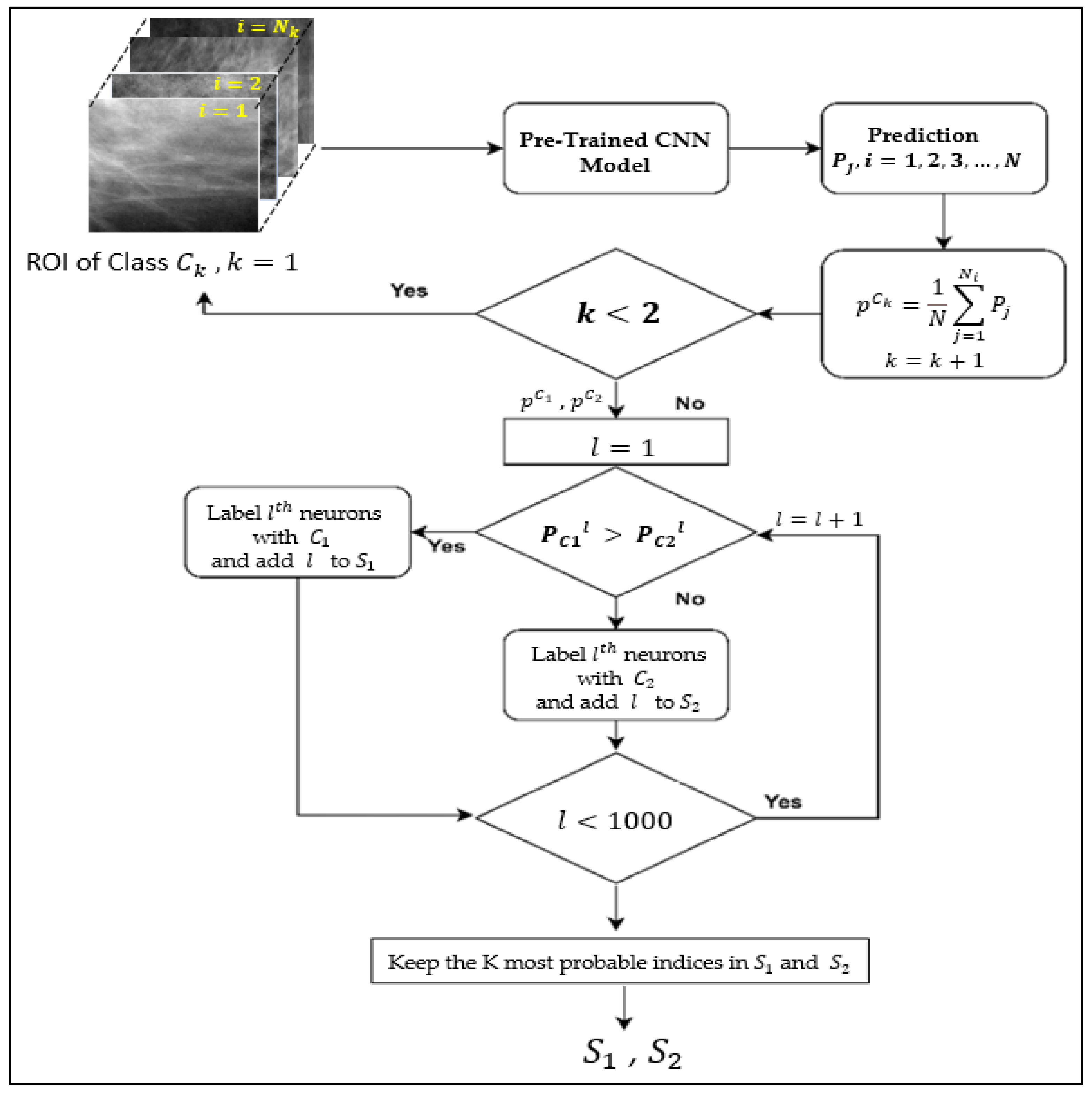
Usually, in deep learning concepts, training refers to learning or fine-tuning the learnable weights and biases. However, in our proposed method, training does not involve learning or fine-tuning the CNN model’s weights and biases. We use a pre-trained model as a backbone model without modifying its architecture and takes classification decisions based on the probability values produced by the classification layer. When an ROI is passed to the CNN model, the different neurons in the output layer with softmax activation give different probability values. The probability values of some neurons are higher than those of others. This means that these neurons can be assigned to the class of the ROI. In view of this, here, training means to determine which neurons in the classification layer give higher probability values for ROIs of a specific class and then associate these neurons with that class. For example, let there be 10 neurons in the classification layer and K = 3. Then, the three (K = 3) neurons (say 3, 4, and 7) that give the highest average probability values for the ROIs belonging to class 1 (benign) are assigned to class 1 and$S_1$ is set to {3, 4, 7}. Similarly, the three (K = 3) neurons are assigned to class 2 (malignant) and$S_{2 }$is determined, say,$S_2$ = {1, 6, 9}. Training here means to determine$S_1$ and$S_2$using the training data.

The algorithm for assigning neurons in the classification layer to classes 1 and 2 is described in detail below, and its flowchart and pseudocode are depicted in Figure 1 and Algorithm 1.

Algorithm 1: Training Phase (The pseudo code of the training method).

Input: $D$, the training data, and $K, the number of most propable neurons$,$M, a pre-trained CNN model$

Output: The label sets $S_1$ and $S_2$

Processing:

1. Partition $D$into$D_1$and$D_2$ based on the class labels

2. Initialize$S_1=Ø, S_2=Ø$

3. For$i=1, 2$

$p^{C_i}=\left[ \right]$

For each $I \in D_i$

$P$ = M ($I$)

$p^{C_i}=p^{C_i}+p$        EndFor

$p^{C_i}=p^{C_i}/N_i$, $where N_i=\left|D_i\right|$      EndFor

4. $d=dimension of p^{C_1}$

5. For$i=1,2,..,d$

$if p^{C_1}>p^{C_2}, then add i to S_1$

$\mathit{e}\mathit{l}\mathit{s}\mathit{e} add i to S_1$         EndFor

6. Keep in$S_1\mathrm{and} S_2 the indices of the K$most probable neurons

We have two classes: benign ($C_1)$ and malignant ($C_2)$; thus, the neurons in the classification layer are to be labelled as belonging to class $C_1$ or $C_2$. In the training phase, the training dataset is partitioned into two sets ($D_1 \mathrm{and} D_2)$ according to their class labels, so we have two training sets, the first set $D_1$ contains benign ROIs, and the second set $D_2$ contains malignant ROIs.

First, the ROIs in $D_1$ of the benign class ($C_1)$are passed to a pre-trained CNN model, and their predictions are calculated as probability vectors. The dimension d of this vector is usually 1000 because most of the available pre-trained CNN models are trained for the ImageNet dataset, which consists of 1000 classes. The neurons in the classification layer are labeled based on these probability vectors, i.e., the label sets $S_1$ and $S_2$ are determined. Specifically, let $D_1=\left\{ I_1^1,I_2^1,\dots ..,I_{N_1}^1\right\}$ be the training set consisting of $N_1$ benign ROIs. Each $I_i^1$ is passed to the backbone pre-trained CNN model $f$, which yields the probability vector $p_i={\left[p_1^i, p_2^i, \dots , p_d^i\right]}^T$ i.e., $f\left(I_i^1\right)=p_i, i=1, 2, \dots , N_1.$ Next, the average probability vector $p^{C_1}$ is calculated, i.e.,:

$$p^{C_1}=\frac{1}{N_1}{\displaystyle \sum }_{i=1}^{N_1}{p}_i={\left[p_1^{C_1}, p_2^{C_1}, \dots , p_d^{C_1}\right]}^T$$

(1)

Similarly, $p^{C_2}$ is computed for the malignant class ($C_2)$.

To determine whether a neuron belongs to class 1 or 2, we compare the corresponding probability values in $p^{C_1} \mathrm{and} p^{C_2}$. For any i, if $p_i^{C_1}>p_i^{C_2}$, then the $i^{th}$ neuron is assigned the label $C_1$ and put in the set $S_1$, the set of labels of the benign class, otherwise it is labeled $C_2$ and put in the set $S_2$, the set of labels of the malignant class. As the number of neurons in the classification layer of pre-trained CNN models is usually 1000, the cardinality of each set will be big and the computation cost in the testing phase will be high. To overcome this issue, we keep only the K most probable indices in S1 and S2. K is the only hyperparameter of the proposed method and its suitable value is determined by experiments considering its different values ${\mathit{S}}_{\mathit{1}}$ and${\mathit{S}}_{\mathit{2}}$. Note that ${\mathit{S}}_{\mathit{1}}$ ∩ ${\mathit{S}}_{\mathit{2}}$ = $\mathrm{Ø}$ due to the condition $p_i^{C_1}>p_i^{C_2}$, i.e., ${\mathit{S}}_{\mathit{1}}$ and${\mathit{S}}_{\mathit{2}}$do not overlap.

The diagram in Figure 1 depicts the specifics of this phase, and pseudocode is also provided.

The output of the training phase is the sets ${\mathit{S}}_{\mathit{1}}$ and ${\mathit{S}}_{\mathit{2}}$, which include the labels of the neurons belonging to the benign or maliganant class. The computational cost of this phase is very low. It requires only a single pass through the pre-trained CNN model for each training example and then goes through the prediction probability of each neuron to label it. The time required to complete the process, including the training and testing phases, depends on the CNN model’s architecture. For instance, Vgg16 requires approximately one minute to complete the one-fold process (as its architecture is very simple and the number of layers are also low). GoogleNet takes approximately two minutes. One-fold computation does not exceed three minutes across all models.

3.3. Testing Phase

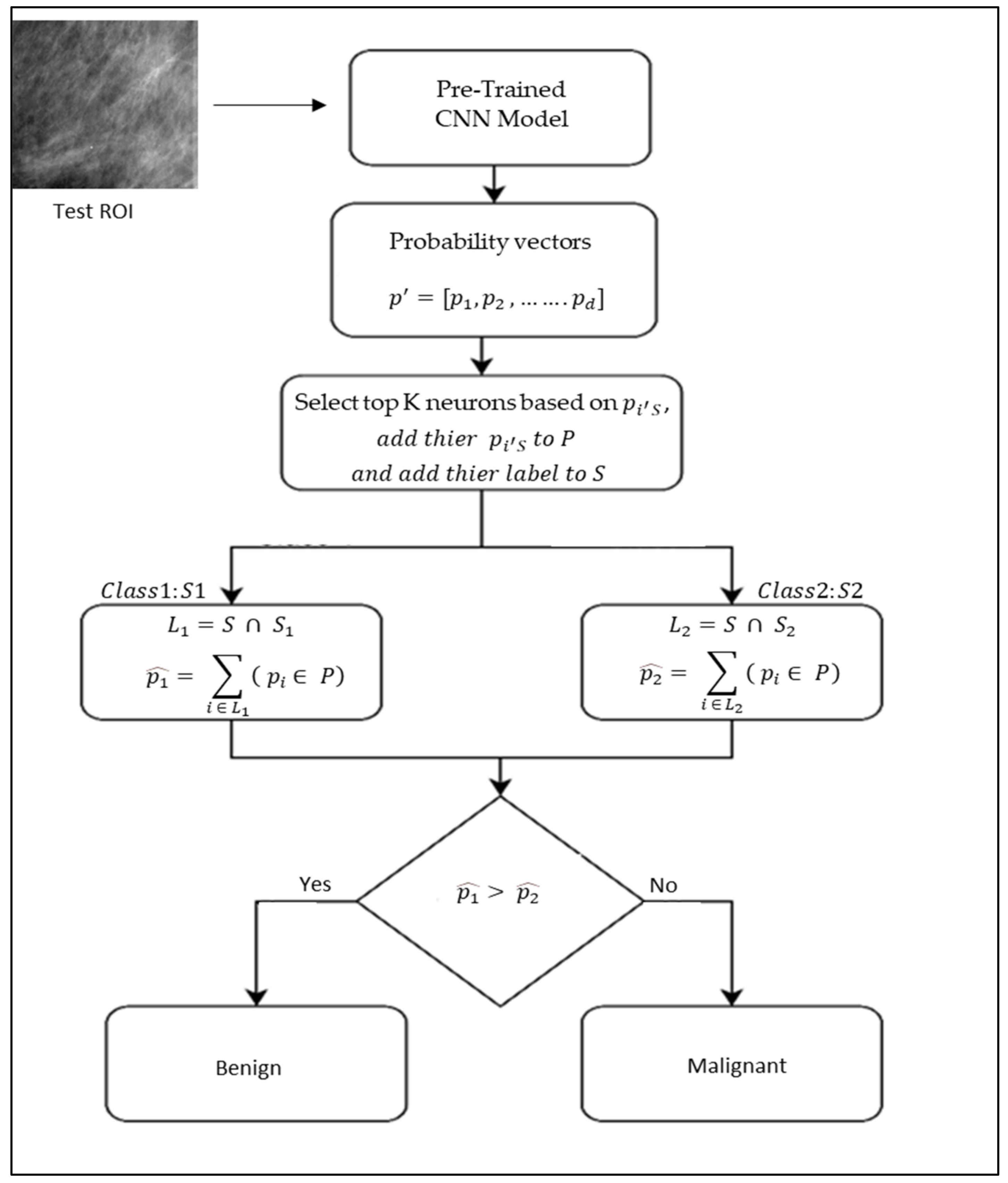
Typically, testing in deep learning involves passing an image to a trained model and then predicting its label by computing the most probable neuron. In our case it is different. We pass an unknown mass ROI to the backbone CNN model, find the K most probable neurons and determine the predicted label based on these neurons. For example, let there be 10 neurons in the classification layer and K = 3. Then, we find the three most probable neurons (say 3, 6, 7) and set S to {3, 6, 7}. After that, we compute $L_1=S \cap S_1$ = {3, 7} and $L_2=S \cap S_2$ = {6}, where $S_1$ and $S_2$ are determined in the training phase. Finally, using the indices in $L_1$ and $L_2$, we calculate the probabilities $\widehat{p_1}$ = $p_3$ + $p_7$, and $\widehat{p_2}$ = $p_6$. If $\widehat{p_1}$ > $\widehat{p_{2 }}$, then the predicted class is 1 (benign), otherwise, it is class 2 (malignant).

This phase predicts the benign or malignant label of an unknown ROI I based on the labels of the neurons in the classification layer of a pre-trained model, which are associated with each class in the training phase. The algorithm for predicting the label of an unlabeled ROI is described in detail in the following paragraph, and its flowchart is depicted in Figure 2 and Algorithm 2.

Algorithm 2: Testing Phase (The pseudo code of the testing method).

Input: An ROI$I$,$M, the pre-trained CNN model, S_1, S_2, K$

Output:Label of$I$

Processing:

1. $\mathit{P}$ = M ($I), where P={\left[p_1,p_{2 }, \dots \dots .p_d\right]}^T$

2. Find$K$most probable neurons using$\mathit{P}$,Put their indices to$S$and their probabilities to$P$

3. For $i=1,2$

$L_i=S \cap S_i$

$\widehat{p_i}=\frac{1}{\left|L_i\right|}\sum _{j=L_i}\left(p_j\in P\right)$       EndFor

4. $\mathit{i}\mathit{f} \widehat{p_1}>\widehat{p_2}, then label of I is Benign otherwise, its label is Malignant$

First, an unknown ROI I is passed to the backbone CNN model $f$, which yields the probability vector $p^{\prime }=\left[p_1,p_{2 }, \dots \dots .p_d\right]$, calculated using the softmax layer. Based on the probability values of $p_i\prime s$, the top K most probable neurons of the last FC layer are selected, and their corresponding $p_i$ values are added to the set P of probability values, and their labels are added to the set of labels S, i.e., $P=\left[ p_1,p_2,.., p_K\right], \mathrm{S}=\left[ I_1,I_2, .., I_K\right]$. Next, we determine how many neurons belong to class 1 and how many belong to class 2 out of K selected neurons (to select the values of K, in the training phase, we compute the performance of the model at many different K values and then select the value of K that gives the best result in the training phase to apply to the testing data); to avoid a tie, we consider odd values of K only. To accomplish this, we take the intersection of S with S₁ and S₂ that is computed during the training phase. It yields the sets of labels $L_1=S \cap S_1$ and ${\mathrm{L}}_2=\mathrm{S} \cap { \mathrm{S}}_2$, which contains the labels of the selected neurons that belong to class 1 and class 2. Using the labels in L1 and the set of probability values P, we select the $p_i\prime s$ of the neurons belonging to class 1; using these probability values, we compute the probability $\widehat{p_1}$, i.e., $\widehat{p_1}=\sum _{i \in L_1}\left(p_i\in P\right)$. Similarly, we compute the probability $\widehat{p_2}$for class 2$, \mathrm{i}.\mathrm{e}., \widehat{p_2}=\sum _{i \in L_2}\left(p_i\in P\right)$. Finally, we compare $\widehat{p_1}$ and $\widehat{p_2}$. If $\widehat{p_1}>\widehat{p_2}$, then the predicted class of I is class 1 (benign). Otherwise, its class is class 2 (malignant). Notably, the final decision in this case is based on the activation of multiple neurons, making it more stable than a decision based on the activation of a single neuron.

The computational cost of this phase is extremely low. It requires one pass through the backbone CNN model for the ROI, selecting top K neurons, and finding the labels of neurons belonging to classes 1 and 2.

4. Evaluation Protocol

We used the DDSM dataset for all experiments. We implemented the code using Matlab 2020 as a software to train, validate, and test the performance of our proposed method. We performed experiments on a computer equipped with an Intel(R) Core(TM) i9-9900k CPU @ 3.60 GHz, RAM 64.0GB.

4.1. Dataset

We performed experiments using the benchmark the public domain Digital Database for Screening Mammography (DDSM) [21] and INbreast [22] datasets.

4.1.1. DDSM

DDSM has been extensively utilized by other researchers, allowing us to compare our results with theirs. The dataset includes numerous types of abnormalities, including masses and calcification. Additionally, it has annotations for mass ROIs. In addition to the ROI image, the dataset includes the entire mammography image in DICOM format. The ROIs are recognized by the experts, extracted, and delivered with the dataset. Therefore, in this situation, no further process is required to extract the ROIs; these ROIs are used for training and testing. In this study, we selected a subset of the dataset containing only ROIs for masses, as the research is limited to identifying masses as being benign or malignant. The subset of the data set includes 512 mammography pictures, 256 of which are malignant and 256 of which are benign.

4.1.2. INbreast

The Inbreast [22] dataset was supplied by the Breast Centre at the University Hospital of So Joo in Portugal; it is accessible to the public and contains 115 cases with 410 images. In 90 cases, both breasts are affected (4 images per case), whereas the remaining 25 are from mastectomy patients (2 images in each case). Numerous forms of abnormalities are included, such as masses and calcifications. Annotations of the ground truth created by professionals were also included.

Each dataset used in the experiments and evaluation of the proposed method contains mammography images together with expert radiologists’ annotations specifying the location and kind of masses. Using this annotation, mass ROIs were cropped and utilized in studies.

4.2. Method of Evaluation

We evaluated the proposed methods by executing different experiments using 10-fold cross-validation. We divided the ROIs into 10 folds of approximately equal sizes. For each experiment the proposed method was trained and tested 10 times, and the average performance measures were calculated. Each time, one of the folds is excluded from the training process, but the excluded fold is used to calculate the performance of the model after training. Thus, the ROIs’ bias and sensitivity are minimized, and more precise results are obtained [23].

4.3. Metrics for Evaluation

We used five performance metrics, i.e., accuracy, sensitivity, specificity, F1-Score, and execution time, to evaluate the performance of the proposed method. These metrics are defined as follows:

$$Accuracy=\left(TP+TN\right)/\left(TP+TN+FP+FN\right)$$

(2)

$$Sensitivity=TP/\left(TP+FN\right)$$

(3)

$$Specificity=TN/\left(TN+FP\right)$$

(4)

$$F1-Score=2\left(Sensitivity \ast Specificity\right)/\left(Sensitivity+Specificity\right)$$

(5)

where TP is the number of true positives, TN is the number of true negatives, FP is the number of false positives, FN is the number of false negatives, and execution time is the average time taken to process and test one image.

5. Experimental Results

The K is the parameter of the method. To find which value of K is more effective and efficient, we performed experiments with different values of K. There are different CNN models based on different architectures. We examined different pre-trained CNN models, which were pre-trained on the ImageNet dataset. We tested the widely used CNN models, such as GoogleNet, DenseNet-121, ResNet-101, ResNet-152, ResNet-50, VGG16, and VGG19. Multiple experiments were conducted using these CNN models and different values of K.

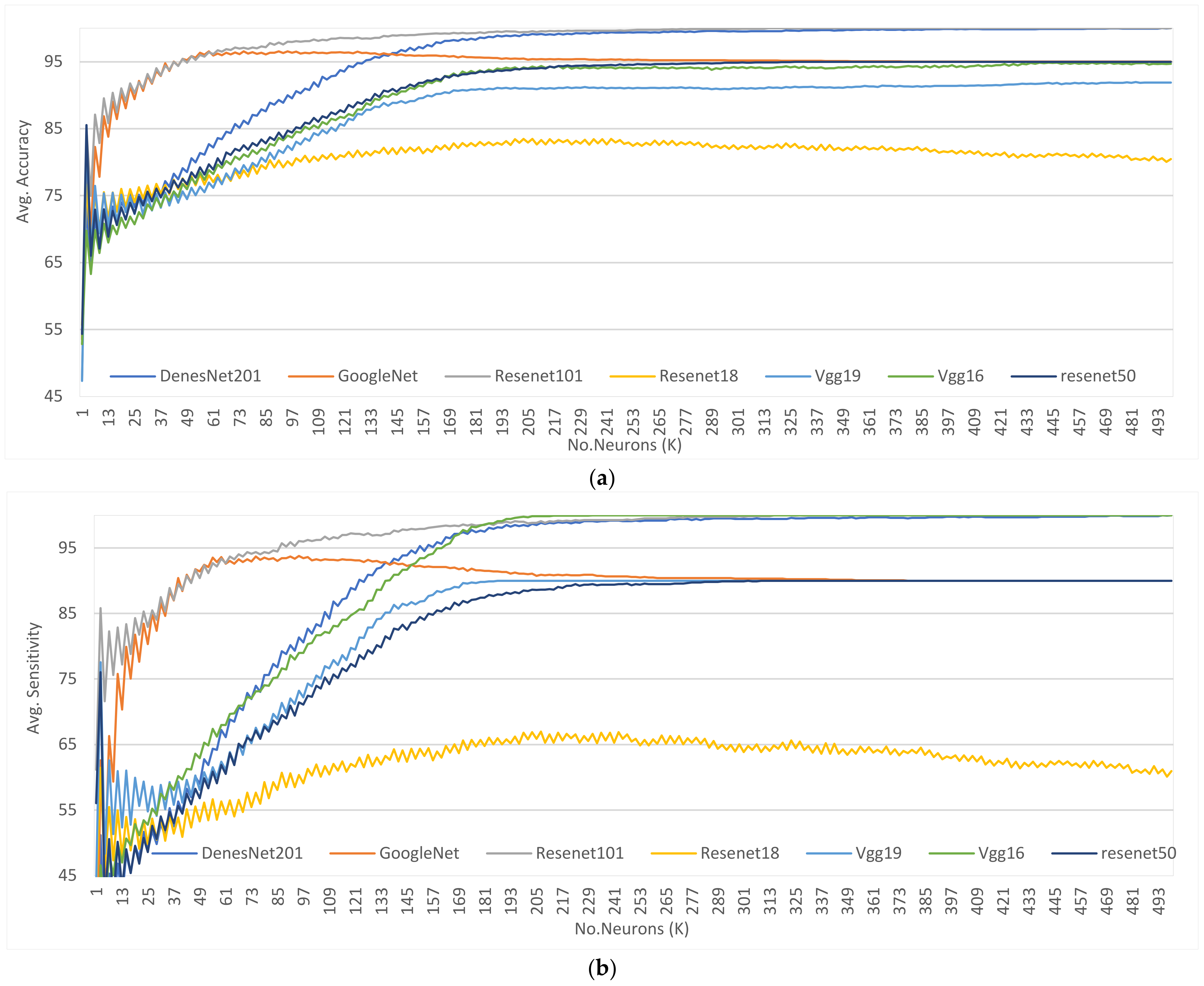
The charts in Figure 3 show the accuracy, sensitivity, specificity, F1-Score, and average execution time results for different values of K and different CNN models.

In the following sections, we discuss the results in detail.

5.1. Effect of Different Values of K

In this section, we explore the effectiveness of K and how to determine and conclude the best K value. Then, we evaluate the performance of backbone CNN models with the selected K. To determine the best value of K, we performed experiments with a single backbone CNN model. More detailed information is discussed in the subsequent sections.

5.1.1. Analyzing the Best Value of K for One Model

To determine the best K value, we examined all potential K values (K = 1,3,…, d; d = 1000) for DenseNet-121. We selected DenseNet-121 as our backbone model since it is reported to outperform the other CNN models in the ImageNet dataset [24]. Then, we apply this value of K for the rest of the CNN models. The following figure shows the performance with DenseNet-121 for different values of K.

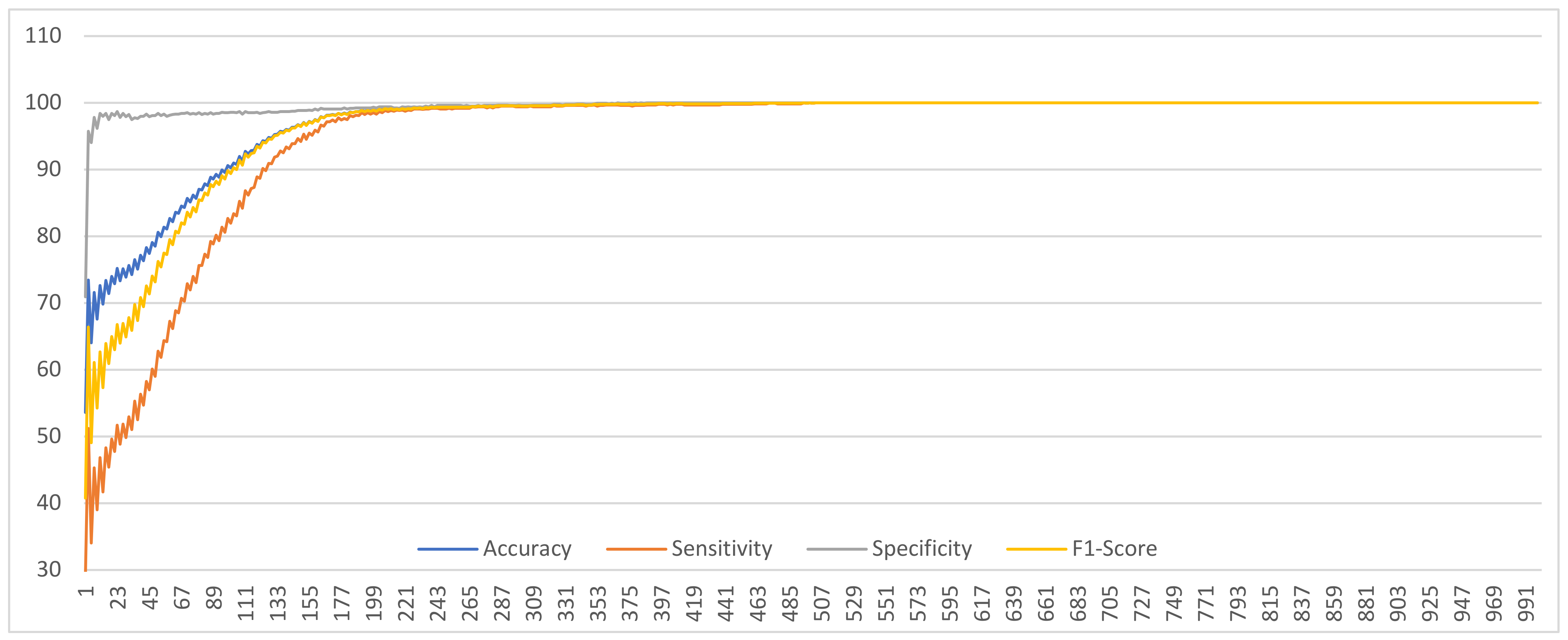
The graphs in Figure 4 illustrate the performance of the proposed method with DenseNet-201 as a backbone model in terms of accuracy, sensitivity, specificity, and F1-Score. We may observe that when K is very low, performance is generally poor. When K equals 495, all performance indicators attain their maximum value. The performance then remains constant for greater values. This suggests that the model is stable when K is close to 500.

5.1.2. Analyzing the Performance of Other Backbone CNN Models When Applying the Best Value of K

The graphs shown in Figure 3a–e show the performance measures for accuracy, sensitivity, specificity, F1-Score, and execution time for different CNN models against different values of K.

In general, as the value of K increases, the performance is increased. The average accuracy hits a low point when K =1 then, it significantly increases in all models for all values of K until it reaches the maximum, after which it may fluctuate.

Table 2. The value of K that gives the best performance for all CNN models individually.

Performance Metric	ResNet-101	DenseNet-121	GoogleNet	ResNet-18	ResNet-50	VGG16	VGG19
Accuracy	315	495	75	207	431	443	483
Sensitivity	315	495	95	207	303	443	483
Specificity	315	495	243	207	431	3	483
F1-Score	315	495	59	207	431	443	483

shows the best values of K, which give the best performance for different CNN models in terms of accuracy, sensitivity, specificity, and F1-score.

The average accuracy, sensitivity, and F1-Score for ResNet-18 are at their highest when K is between 200 and 250, after which it fluctuates little. GoogleNet exhibits similar behavior, but its peak value of K is different. GoogleNet reaches its peak performance when K is between 50 and 80. Vgg16, Vgg19, ResNet-50, ResNet-101, and DenseNet-121 exhibit identical behavior; when the value of K is increased, performance is always improved, but with slight variations. ResNet-18 underperforms all other models, according to the graphs, whereas DenseNet-121 and ReseNet-101 outperform it. Vgg16 provides the second-best results followed by GoogleNet and ResNet-50. Vgg19 performs better than ResNet-18 but is inferior to ResNet-50 and GoogleNet. All trend values for models lie between 65% and 100%.

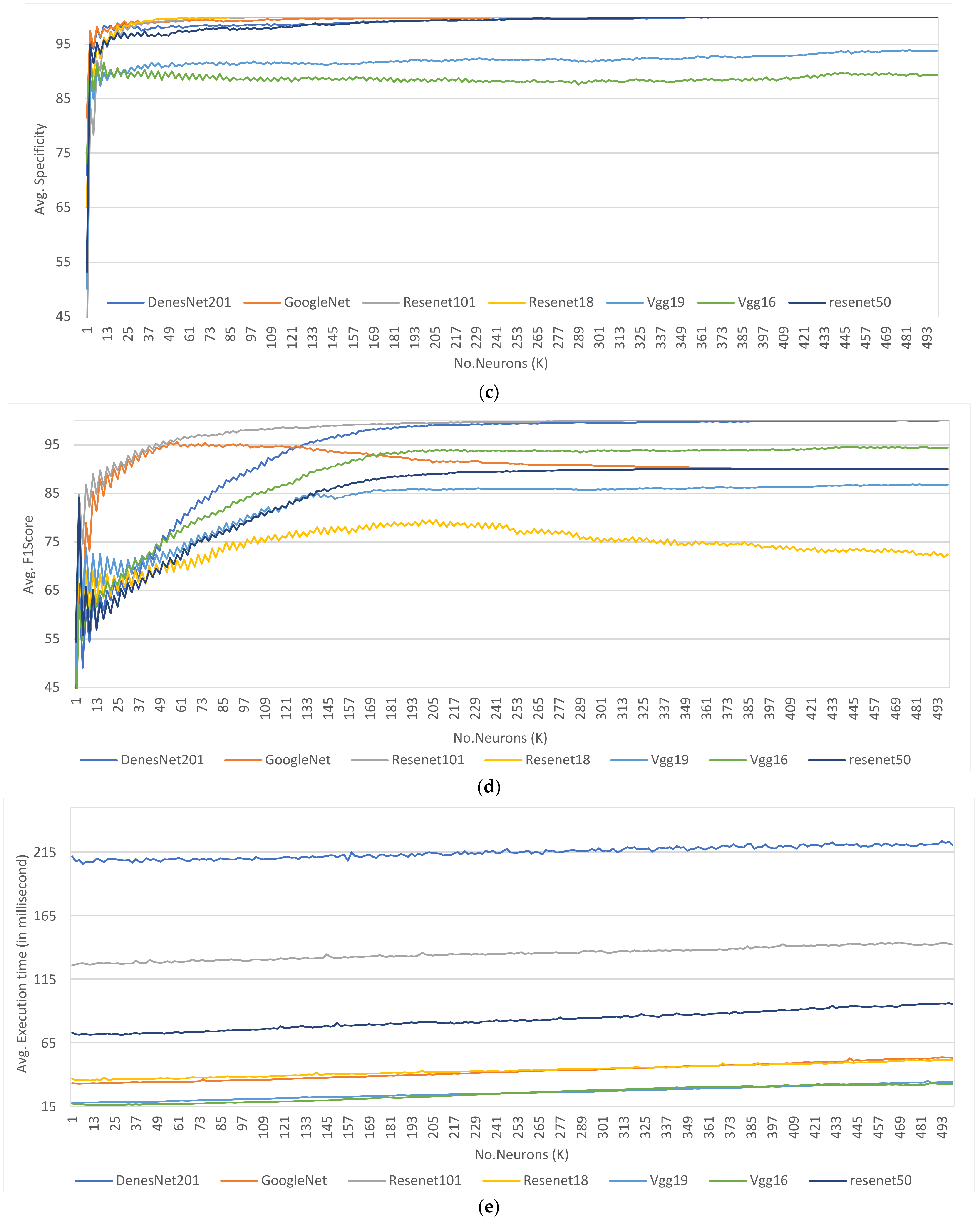
For specificity, all models show the same behavior. The performance increased when the value of K is increased with fluctuations. The trend values fall between 85 and 100%. Vgg16 and Vgg19 underperform while all the others outperformed.

For testing time, in general, the average testing time is increased linearly when the value of K is increased. The graph shows that the testing time using Vgg16 and Vgg19 is the lowest while ReseNet-101 is the highest. GoogleNet and ResNet-18 are the next. Then, DenseNet-121. The worst is ReseNet-101.

As sensitivity is the most important metric for breast cancer classification problems, it would be preferable to select the value of K that produces the best sensitivity results for the majority of models. Alternatively, if specificity is the most important factor, the optimal value of K would be the one that maximizes specificity.

ResNet-101 and DenseNet-121 are the best models, while ResNet-18 is the worst. ResNet-101 and DenseNet-121 achieved the best performance across all metrics compared to all other models. ResNet-101 and DenseNet-121 have peak performance for all metrics at K = 315 and 495 for ResNet-101 and DenseNet-121, respectively. They are also more resistant to variations in the value of K. This is a significant benefit for CNN model selection, as only ResNet-101 and DenseNet-121 models can produce the best results across all metrics. When the value of K is 495, both ResNet-101 and DenseNet-121 give the best performance. In addition,

Table 3. The value of K that gives the best performance for all CNN models individually.

CNN Model	Accuracy			Sensitivity			Specificity			F1-Score
	K			K			K			K
	Best K Value	495	315	Best K Value	495	315	Best K Value	495	315	Best K Value	495	315
ResNet-101	100	100	100	100	100	100	100	100	100	100	100	100
DenseNet-121	100	100	99.54	100	100	99.41	100	100	99.66	100	100	99.53
GoogleNet	96.55	95	95.17	93.78	90	90.34	100	100	100	95.52	90	90.65
ResNet-50	95	95	94.87	90	90	90	100	100	99.75	90	90	89.87
ResNet-18	83.48	80.58	82.44	66.97	61.17	64.87	100	100	100	79.54	72.62	75.67
VGG16	94.87	94.66	94.03	100	100	100	92.94	89.32	88.07	94.6	94.36	93.66
VGG19	91.97	91.89	91.18	90	90	90	93.94	93.78	92.35	86.85	86.76	85.98

compares the results with three different values of K (K = the best value provided by the individual model, Table 2; K = 495—the best value provided by DenseNet-121; K = 315). The results in the table demonstrate that when K = 495, the obtained results are marginally superior to when K = 315. We concluded that the optimal value of K is 495.

On the other hand, we also tested that S₁ and S₂, as given in the training phase, are non-overlapping. As an example, S₁ and S₂ for an ROI when using DeneseNet-201 with K = 11.

$$S_1=\{981,284,333,819,962,910,906,280,557,112,420\}$$

$$S_2=\{886,975,978,701,912,905,563,795,592,979,490\}$$

We can see that the intersection between those two sets is empty.

5.1.3. Analyzing the Effect of Different CNN Models

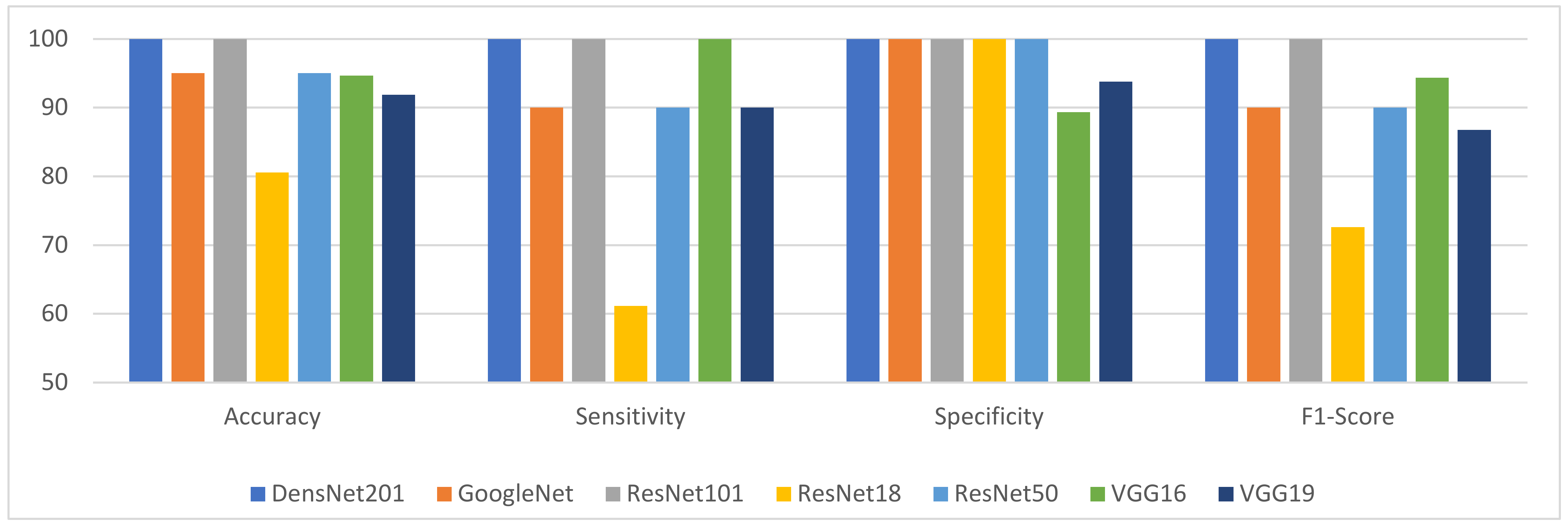
Figure 5 and Figure 6 illustrate the effect of the various pre-trained CNN models on the proposed method when utilizing the best value of K (495) on the DDSM and INbreast datasets, respectively. They demonstrate that ResNet-101 and DenseNet-201 consistently give the best results across all KPIs considered (accuracy, sensitivity, specificity, and F1-Score). The graphs also reveal that ResNet-18 yields the worst results in terms of accuracy, sensitivity, and F1-Score. ResNet-18 is the worst model, while ResNet-101 and DenseNet-201 are the best.

ResNet-101 and DenseNet-121 models produce the best results in terms of accuracy, while ResNet-18 has the worst. Vgg19 is superior to ResNet-18 but inferior to all other models. In DDSM, GoogleNet, ResNet-50, and Vgg16 are ranked second with a slight difference because they produce nearly identical results. While on INbreast, Vgg16 shows poorer results than GoogleNet and ResNet-50, but it is better than Vgg19.

In terms of sensitivity, the results of the analyses of both datasets are extremely similar. Utilizing the ResNet-101, Vgg16, and DenseNet-121 models, the proposed method yielded the most effective results. GoogleNet, Vgg19, and ResNet-50 follow. These three models produced identical outcomes. The variance between these three models is not significant. The CNN model named ‘ResNet-18′ ended in last place, and its sensitivity result was the worst.

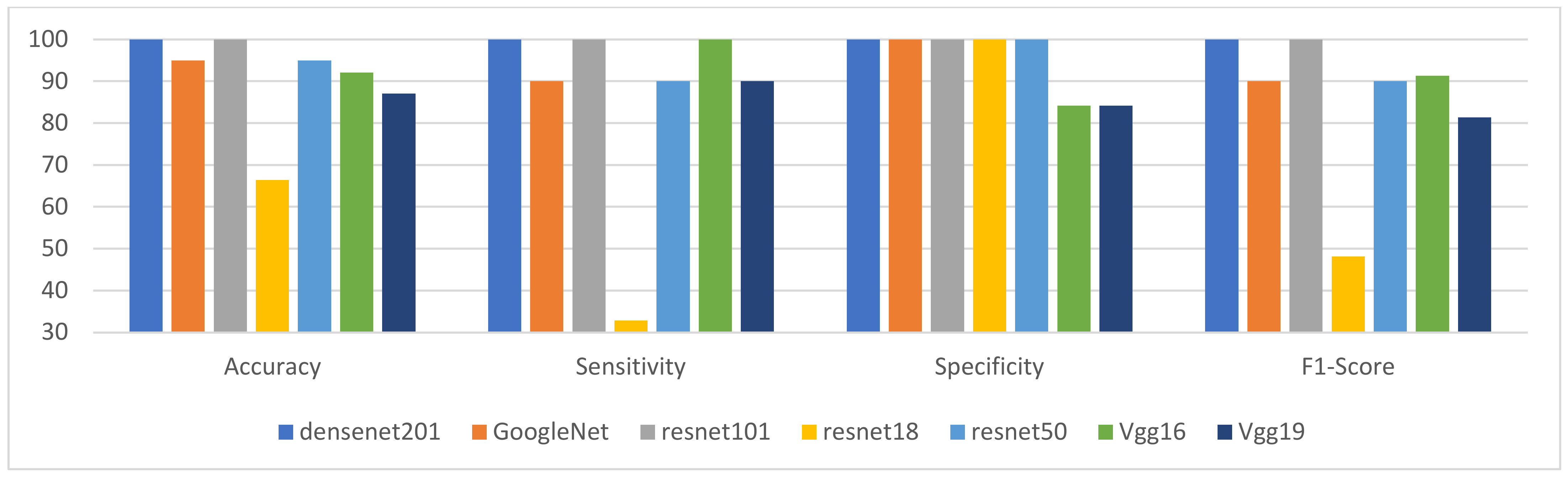
In terms of specificity, the DenseNet-201, GoogleNet, ResNet-18, ResNet50, and ResNet-101 results are the best and equal to 100% in both datasets. Vgg19 ranks second in DDSM with a value of 93.78%. The worst performance is given by Vgg16, which is approximately 89.32%. In the INbreast dataset, both Vgg16 and Vgg19 produce an accuracy of approximately 84%, the lowest of all models.

Both datasets exhibited the same behavior for F1-Score, which is very similar to the behavior of sensitivity. DenseNet-121 and ResNet-101 achieved a perfect score of one hundred percent for their performance. Vgg16 ranks second with approximately 94%. GoogleNet and ResNet-50, with performance results around 90%, are third. Vgg19 is ranked fourth, and ResNet-18 is ranked last, with approximately 72% and 48% accuracy for the DDSM and INbreast datasets, respectively. In terms of execution time, Figure 3e depicts the average execution time for a single image.

In general, increasing the value of K increases the processing time. However, the difference is insignificant and hardly noticeable. DenseNet-121 required the longest execution time among the CNN models, whereas Vgg16 and Vgg19 required the least. This is due to the CNN architecture. For Vgg16 and Vgg19, the model is simple and the number of learnable layers does not exceed 19, whereas for ResNet-101, the maximum number of learnable layers is 201. The subsequent model, ResNet-101, required more time than ResNet-50. As the number of learnable layers for ResNet-101 and ResNet-50 is 101 and 50, respectively (more than 19), it is logical that they require more time than Vgg19. In terms of execution time, ResNet-18 and GoogleNet are very similar and are considered the second-best models. DenseNet-121 required more than twice as many ×10 operations as Vgg16, but it is still fast as the time is measured in milliseconds and is still less than one second.

On the basis of these analyses, we can conclude that the ResNet-101 and DenseNet-121 models are the best backbone models for the proposed method that result in the best classification results for breast cancer mass. Using the above analysis and the following graph, it can be concluded that the ResNet-101 and DenseNet-121 models are the best models for solving the breast cancer image classification problem with our proposed method. Comparing the accuracy of the proposed method to that of the related works presented in the related works section and Table 1, the proposed method yielded the best result, i.e., 100%.

Table 4. Summary of the performance of the proposed method for K = 495 and different backbone CNN models on the DDSM dataset.

CNN Model Name	Accuracy ± SD	Sensitivity ± SD	Specificity ± SD	F1-Score ± SD
DenseNet-121	100 ± 0	100 ± 0	100 ± 0	100 ± 0
ResNet-101	100 ± 0	100 ± −0	100 ± 0	100 ± 0
ResNet-50	95 ± 15	90 ± 30	100 ± 0	90 ± 30
ResNet-18	80.59 ± 10.78	61.18 ± 21.55	100 ± 0	72.63 ± 24.75
GoogleNet	95 ± 15	90 ± 30	100 ± 0	90 ± 30
Vgg16	100 ± 0	90 ± 30	93.78 ± 3.15	86.76 ± 28.95
Vgg19	91.89 ± 14.01	100 ± 0	89.33 ± 5.24	94.36

and

Table 5. Summary of the performance of the proposed method for K = 495 and different backbone CNN models on the INbreast dataset.

CNN Model Name	Accuracy ± SD	Sensitivity ± SD	Specificity ± SD	F1-Score ± SD
DenseNet-121	100 ± 0	100 ± 0	100 ± 0	100 ± 0
ResNet-101	100 ± 0	100 ± 0	100 ± 0	100 ± 0
ResNet-50	95 ± 15	90 ± 30	100 ± 0	90 ± 30
ResNet-18	66.42 ± 5.47	32.84 ± 10.94	100.00 ± 0	48.12 ± 16.03
GoogleNet	95.00 ± 15	90.00 ± 30	100.00 ± 0	90.00 ± 30
Vgg16	92.09 ± 2.63	100.00 ± 0	84.19 ± 5.27	91.33 ± 2.88
Vgg19	87.09 ± 12.36	90.00 ± 30	84.19 ± 5.27	81.33 ± 27.11

Summary of the performance of the proposed method for K = 495 and different backbone CNN models on the DDSM and Inbreast dataset respectively.

Figure 5. Comprehensive view on DDSM dataset of the effect of the different CNN models using best value of K.

Figure 5. Comprehensive view on DDSM dataset of the effect of the different CNN models using best value of K.

Figure 6. Comprehensive view on INbreast dataset of the effect of the different CNN models using best value of K.

Figure 6. Comprehensive view on INbreast dataset of the effect of the different CNN models using best value of K.

6. Discussion

Common CNN backbone models, such as GoogleNet, DensNet-201, ResNet-101, ResNet-152, ResNet-50, Vgg16, and Vgg19, are utilized by the proposed method.

As observed in the Results section, DenseNet201 and ResNet-101 outperform all other models.

In the architecture, DenseNet201 receives further input from all preceding layers and passes its own feature-maps to all subsequent layers. Each layer acquires “collective knowledge” from the layers underneath it. Since each layer receives all preceding layers as input, this results in more diverse features and typically more rich patterns. Additionally, it aids in reducing the amount of learnable parameters. ResNet101 uses “skip connections” and features heavy batch normalization. The skip connection method enables the model to train a network with deeper layers. These features enable DenseNet-201 and ResNet-101 to achieve superior results. In terms of the amount of learnable parameters, DenseNet-201 requires fewer parameters than ResNet-101. Consequently, DenseNet is regarded as a superior architecture.

GoogleNet employs groups of inception models, each of which includes pooling, convolutions at different scales, concatenation operations, and 1x1 feature convolutions that function as feature selectors. In addition, batch normalization, picture distortions, and RMSprop were utilized. GoogleNet employs fewer parameters than Vgg16 and Vgg19, and neither Vgg16 nor Vgg19 use batch normalization. This explains why GoogleNet typically returns better results than Vgg16 and Vgg19. Although ResNet-18 has more sophisticated techniques than Vgg19 and Vgg16, it underperformed in all CNN models.

As discussed in Section 2, the majority of available algorithms for mass categorization rely on machine learning or deep learning to solve the problem. For the deep learning strategy, they either utilize end-to-end training or transfer learning with or without fine-tuning.

It requires a domain expert to manually decide and extract the features for the hand-crafted approach to produce a satisfactory result. On the other hand, the deep learning approach can automatically extract features and learn new features, but it requires a massive amount of training data to train the model. This constraint was overcome by the fine-tuning method, but it still required training data and computational machines.

Despite the fact that state-of-the-art approaches have attained high performance, the majority of them require advanced deep learning solutions to solve several challenges. Deep learning requires massive amounts of data to train the model or else the model will be overfit. However, rich data are unavailable due to the absence of available medical images. Although the data augmentation strategy is used to address this issue, when adding extra data, we must ensure that the new data are likewise appropriately generated and labeled. Otherwise, incorrect learning may occur, leading to a decrease in performance. In addition, the computational time and expense will increase.

The number of learnable parameters also presents an issue.

One of the challenges with using a deep convolutional model is that it must be trained on a large number of parameters, and there is a considerable risk of overfitting and lack of generalization. In addition, deep learning algorithms require high-performance hardware and training time for the model.

To the best of our knowledge, this is the first approach in the literature that uses deep learning to classify mass ROIs without requiring any modifications. No additional data were utilized, and no specific training equipment was required. We suggested a low-cost, straightforward approach for classifying mass ROIs as benign or malignant. Therefore, this method does not require extensive parameter learning. In addition, a small number of training data are sufficient to train the deep CNN model. Moreover, it can achieve state-of-the-art results with fewer requirements.

Table 6. Performance comparison between proposed method and state-of-the-art on DDSM dataset.

Reference	Method	Acc	Sens	Spec
Nagarajan et al. [16] (2019)	GLCM and GLRM from (MBEMD) and SVM/LDA	93.3
Sun et al. [13] (2019)	CNN with dilated CONV layers	82.02
Lazaros et al. [18] (2021)	Unet for segmentation, CNN	76.8
Meng Lou et al. [20] (2021)	CNN	76.9	77.7	79.3
Shakeel, S et al. [5] (2021)	CNN as feature extraction, SVM as classifier	88.7	84.1	93.0
El Houby et al. [6] (2021)	CNN	91.2	92.3	90.0
Proposed Method	CNN	100	100	100

and

Table 7. Performance comparison between proposed method and state-of-the-art on INbreast dataset.

Reference	Method	Acc	Sens	Spec
Singh, H. et al. [4] (2022)	Relief-F as feature selection, K-NN as classifier	90.4	92.0	88.0
Meng Lou et al. [20] (2021)	CNN	84.5	77.2	88.2
Ahmed et al. [7] (2022)	CNN as feature extractor and Softmax as Classifier	97.1	96.3	97.9
Sannasi et al. [19] (2022)	CNN as features extractors, SVM as Classifier	96.6
El Houby et al. [6] (2021)	CNN	96.5	96.6	96.5
Proposed Method	CNN	100	100	100

compares the performance of the proposed technique to the state-of-the-art on the DDSM and INbreast datasets. The comparison shows that the proposed method is more effective in classifying the mass ROIs using pre-trained CNN models as backbone models.

7. Conclusions

In this study, a novel classification algorithm for benign or malignant mass ROIs on mammography images has been developed. It uses a deep CNN model as a backbone model. Though CNN models demonstrated exceptional performance in numerous applications, the limited availability of annotated data is one of the obstacles typically encountered by researchers attempting to solve problems with medical images using deep learning. There are two strategies proposed in the literature for overcoming this limitation: data augmentation techniques and transfer learning. Although these strategies aid in resolving the issue, they do have limitations. In data augmentation, for instance, the new sample is generated during the training phase. False labeling will cause the misclassification problem and reduce the performance of the model. Thus, we must ensure that these new samples are generated and labeled correctly. In addition, both the computational time and cost are increased.

According to an alternative viewpoint, transfer learning must refine certain parameters and eliminate the FCL entirely. This results in ignoring the pre-trained learning parameters in the removed layer and necessitates the retraining of the parameters in the newly added layer. To address the aforementioned issues, we suggested a simple method for classifying mass ROIs as benign or malignant. The suggested technique utilizes a pre-trained CNN model as a backbone. Instead of removing the final fully connected layer and adding new problem-specific layers, as suggested in the literature, we simply remapped the pre-trained activations to the new classes. The proposed method identifies the neurons with the highest activation in the final fully connected layer and uses those activations to categorize new mass ROIs. The proposed method successfully achieved state-of-the-art results with less computing cost and time than earlier research. We tested the proposed method on two benchmark datasets (DDSM and INbreast) and achieved 100 percent accuracy, sensitivity, and specificity.