
Image Encryption Algorithm Based on a Novel Wide-Range Discrete Hyperchaotic Map


1
School of Mathematics and Computational Science, Guilin University of Electronic Technology, Guilin 541004, China
2
School of Information and Software Engineering, University of Electronic Science and Technology of China, Chengdu 610054, China
*
Author to whom correspondence should be addressed.
Mathematics 2022, 10(15), 2583; https://0-doi-org.brum.beds.ac.uk/10.3390/math10152583
Submission received: 17 June 2022
/
Revised: 15 July 2022
/
Accepted: 16 July 2022
/
Published: 25 July 2022
(This article belongs to the Special Issue Chaos-Based Secure Communication and Cryptography)
Abstract
:Existing hyperchaotic systems suffer from a small parameter range and small key space. Therefore, we propose herein a novel wide-range discrete hyperchaotic map(3D-SCC) based on the mathematical model of the Sine map. Dynamic numerical analysis shows that this map has a wide-range of parameters, high sensitive, high sensitivity of sequences and good ergodicity, which proves that the system is well suited to the field of communication encryption. Moreover, this paper proposes an image encryption algorithm based on a dynamic cycle shift scramble algorithm and image-sensitive function. First, the image feature is extracted by the image-sensitive function to input into the chaos map. Then, the plaintext image is decomposed by an integer wavelet, and the low-frequency part is scrambled by a dynamic cyclic shifting algorithm. The shuffled low-frequency part and high-frequency parts are reconstructed by wavelet, and the chaotic matrix image is bitwise XOR with it to obtain the final ciphertext. The experimental results show that the average NPCR is 99.6024%, the average UACI is 33.4630%, and the average local Shannon entropy is 7.9029, indicating that the statistical properties of the ciphertext are closer to the ideal value. The anti-attack test shows that the algorithm can effectively resist cutting attacks and noise attacks. Therefore, the algorithm has great application value in the field of image encryption.
1. Introduction
1.1. Background
The chaotic system is a non-linear system in which chaotic motion exists. Chaotic motion is a never-repeating, reversible, non-periodic motion generated by a deterministic system with sensitive dependence on initial conditions [1]. Chaotic systems have the characteristics of singular attractor, ergodicity and internal randomness [2]. Lyapunov Exponent (LE) is the rate of the exponential separation with the time of initially close trajectories, which can judge the appearance of chaotic movement [3]. Chaotic systems have the characteristics of positive Lyapunov exponents. Simple chaotic systems have one positive Lyapunov exponent, while hyperchaotic systems have two or more positive Lyapunov exponents, which mean that the hyperchaotic systems have more complex dynamical behavior and represent more complex topologies [4].
The types of chaotic systems can be classified as continuous chaotic systems and discrete chaotic systems. Continuous chaotic systems are chaotic systems based on the observation of time series, where the state of the system is time-dependent, such as the Lorenz system [5] and Chua’s circuit [6]. Unlike continuous dynamical systems, discrete dynamical systems are special types of dynamical systems whose instantaneous states are described by discrete variables [7], such as Logistic map [8], Henon map [9] and the Sine map [10].
Since Mr. Lorenz proposed Lorenz chaos in 1963 [11], chaos systems have attracted the attention of scholars, and many chaos systems have been proposed. For one-dimensional chaos, there are typical mappings such as Logistic mapping, Tent mapping and Sine mapping. However, although one-dimensional chaos has high computational efficiency, it also has the problems of small parameter range, low complexity and low ergodicity. Therefore, more scholars pay attention to high-dimensional chaos and try to construct more complex chaos with hyperchaotic behavior [12,13,14,15]. Zhongyun Hua et al. proposed a two-dimensional chaotic 2D-SLMM combining Logistic mapping and Sine mapping, which has a wider range of parameters, better ergodicity, hyperchaotic characteristics and relatively low implementation cost [12]. Gholamin, P. et al. proposed a new three-dimensional continuous chaos system, which has a new type of attractor but does not have hyperchaotic behavior [13]. Hongxiang Zhao et al. proposed a high-complexity hyperchaotic system by improving the Henon map [14]. At present, there are few studies on the construction of high-dimensional discrete chaos. This paper proposes a novel discrete three-dimensional hyperchaotic map based on the mathematical model of a Sine map.
With the rapid development of the Internet and computer technology, vast amounts of information are transmitted, stored and shared every day. In recent years, people have paid more and more attention to information security. The mainstream methods to ensure image security are digital steganography, digital watermarking and image encryption. Digital steganography protects image security by hiding secret messages in normal messages [16,17,18]. Digital watermarking protects image security by hiding one or more secret marks in the host media [19,20,21]. Image encryption makes the image a meaningless snowflake image through pixel scrambling and diffusion [22,23,24,25]. This article mainly studies image encryption. In cryptography, confusion and diffusion are two properties of the operation of a secure cipher [10]. In image encryption algorithms, confusion is the operation of changing the pixels value of plaintext. Diffusion is the operation of changing the location of the pixels of plaintext. The ability of the chaos system is to generate pseudo-random sequences with unpredictability, ergodicity and sensitivity, and these characteristics are closely related to the confusion and diffusion principles of modern cryptography. Therefore, chaos systems are often used in image encryption algorithms [11,26,27,28,29,30,31,32,33,34,35].
At present, some encryption algorithms only perform encryption in the time domain, and there is a risk of being deciphered. Therefore, scholars have studied many encryption algorithms performing in both frequency domain and time domain [23,28,31,36,37,38]. Feng-Ping An et al. proposed an encryption algorithm based on adaptive wavelet chaos [36]. This algorithm has a relatively strong anti-attack ability, but the decrypted image is distorted to a certain degree. Shakir H.R et al. proposed an image encryption method based on selective AES coding of wavelet transform and chaotic pixel shuffling [37]. The algorithm is simple and efficient. However, image encryption in the frequency domain may affect the quality of the decrypted image [13,36].
1.2. Motivations and Contributions
For image encryption algorithms based on chaotic mapping, the security depends mainly on the chaotic mapping complexity and the algorithm [39]. However, some existing chaotic mappings have some drawbacks, such as small chaotic range, low complexity and less complex dynamical behaviour. Some of the existing encryption algorithms also have some shortcomings, such as poor flexibility and weak resistance to attacks. Therefore, the main motivations of the work lie in:
- The high-dimensional discrete chaotic map with a large parameter range of hyperchaotic behaviour is designed for an image encryption algorithm, which is rare with existing algorithms.
- Design a dynamic scrambling algorithm that is more difficult to crack than traditional scrambling algorithms.
- Design image-sensitive algorithms for use in an encryption algorithm, which enhance the link between plaintext and ciphertext to resist both differential and plaintext attacks.
- This encryption algorithm should be an image algorithm that performs simultaneous diffusion or obfuscation operations in the frequency and time domains to improve security and efficiency.
- The image encryption algorithm should have the advantage of clear decrypted images, resistance to noise and clipping attacks and the flexibility to encrypt square or rectangular images.
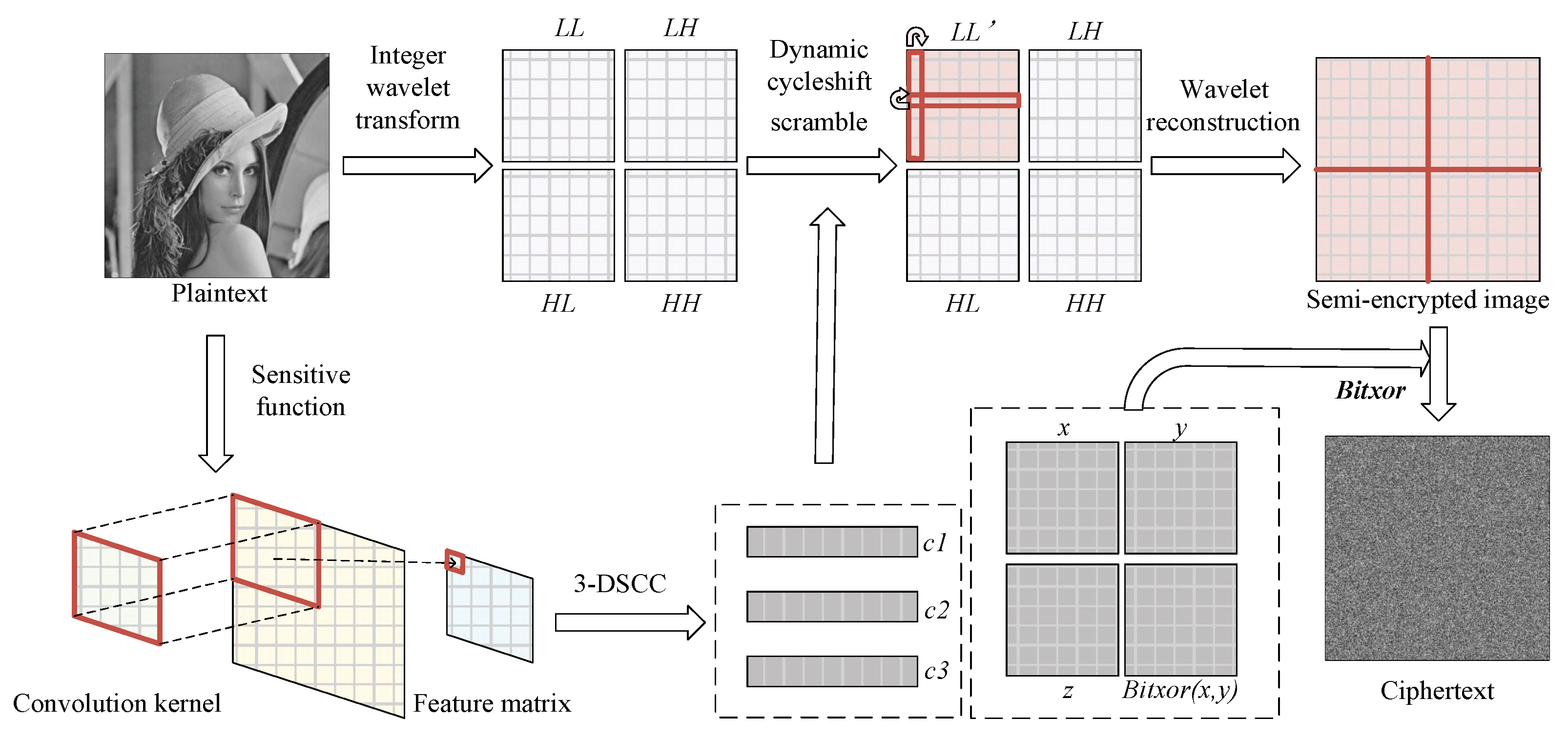
For the above motivations, this paper proposes an image encryption algorithm based on integer wavelet transform and the new discrete hyperchaotic chaotic map. First, it used the proposed sensitivity function to generate the initial value of the novel discrete hyperchaotic map. Then, it performs integer wavelet decomposition on plaintext image, scrambles the low-frequency part by the proposed dynamic cyclic shift scrambling algorithm and performs wavelet reconstruction on the scrambled low-frequency part and high-frequency parts. Finally, it performs bitwise XOR between the reconstructed image and the chaotic matrix to obtain the final ciphertext image.
Section 2 proposes a novel discrete hyperchaotic map and conducts a series of tests on it. Section 3 proposes the sensitive function based on the convolution, the dynamic circle shifting algorithm and the encryption algorithm based on the above algorithm. Section 4 carries out the simulation experiments and security analysis to the ciphertext. Section 5 summarizes and discusses the full text.
2. Mathematical Model and Dynamic Analysis of the Novel Discrete Hyperchaotic Map
The Sine map [5] is a one-dimensional chaos map, which is defined as:
where parameter [0, 1]. The Sine map is chaotic when [0.87, 1].
The Sine map has a small range of parameters, and its sequence is not complex enough, so it cannot meet the requirements of communication encryption. Therefore, inspired by the Sine map, this paper presents a three-dimensional chaotic map. The detailed steps of generating the three-dimensional map are explained as follows. In the first step, two new dimensions are added to the Sine map. To increase the diversity of frequencies, two dimensions are added as cos functions, as Equation (2) shown.
where and are the control parameters.
In Equation (2), these three dimensions are unrelated to each other. Therefore, the three sequences are coupled in the next step. The method of coupling in this paper is to design a perturbation function associated with three dimensions as a perturbation term that is added to the input term in the trigonometric function. Let this perturbation term be g(h,w,z), and the new equation is Equation (3) as shown.
The next step requires adjusting the sequence range and expanding the parameter space. To make the sequence more evenly distributed and have better ergodicity, let the gain term of the trigonometric function be equal to 1, i.e., . At this point, the parameter space needs to be increased, so the gain item in the trigonometric input becomes an adjustable parameter. The new equation, Equation (4), is shown below.
where are the control parameters.
The next step is to discuss the construction of the perturbation function. The output value of the set perturbation function should not be much larger than the value of the sequence . Otherwise, the perturbation term becomes the main determinant of the output value of the sequence. The output values for different input terms should fluctuate up and down in some number, i.e., the output terms are only slightly different. Based on the above conditions, this paper sets up the perturbation function as shown in Equation (5).
where is the numbers close to 0. Since the value range of the sequences is [−1, 1], the output value of the perturbation term fluctuates up and down at 1. Adding a number close to 0 to the denominator is to prevent the denominator from being 0. Substitute Equation (5) into Equation (4) and obtain the new equation as:
where are the control parameters, and , . This paper calls it 3D-SCC for short. It is easy to know that the 3D-SCC is bounded, and the output range is [−1, 1]. Through a trajectory analysis, the Lyapunov exponent, the bifurcation diagram, and a complexity analysis, The 3D-SCC has good chaotic characteristics, such as infinite parameter range, high sensitivity and high complexity.
2.1. Phase Diagrams
The phase diagrams of the 3D-SCC with the parameter and the initial value are shown in Figure 1. It can be seen that the chaotic sequences are almost uniformly distributed in the [−1, 1] space, meaning that the 3D-SCC map has good ergodicity.
Histograms of the 3D-SCC map and the Sine map are exhibited in Figure 2. Two sequences of length 15000 produced by the 3D-SCC map and the Sine map, respectively, are normalised to [0, 1]. Then, we calculate the frequency of each interval to obtain the histogram. As can be observed, the frequencies of the intervals [0, 0.05] and (0.95, 1] are higher than those of other intervals in the histogram of the 3D-SCC map. However, beyond these, the frequencies of other intervals are very close, which can be considered as almost uniformly distributed. However, in the histogram of the Sine map, there are intervals of zero frequency. Therefore, the 3D-SCC map has better ergodicity.
2.2. Lyapunov Exponent and Bifurcation Diagrams
The Lyapunov exponent (LE) and bifurcation diagrams(BD) are the important indicators to verify the dynamic state of chaos [3].
The LE is the rate of the exponential separation with time of initially close trajectories. In this paper, the Jacobian matrix method [40] is used to calculate the Lyapunov exponent of the chaos map in the following situations. Figure 3 shows the LEs and corresponding BD of the Sine map with the initial conditions and . We can notice that the LEs of the Sine map are positive only when , and a wide range of the window period appears in the bifurcation diagram. Figure 3 exhibits the LEs and corresponding BDs of the 3D-SCC map, with the initial conditions and . We can notice that the LE1 and the LE2 are always positive, and there are no window periods in BDs, meaning that the 3D-SCC has a wide range of hyperchaotic behavior in the parameter space. Two parameters are fixed at 2. Figure 4 shows the LEs and corresponding BDs as the remaining parameter changes from 0 to 20. And two parameters are fixed at 100. Figure 5 shows the LEs and corresponding BDs as the remaining parameter changes from 0 to . Interestingly, as one of the system parameters increases, the LE value of the chaotic map increases. Moreover, the three LE values are positive with an infinite range of parameters, which is not common in other discrete chaotic map models. It shows that the system has a high degree of chaos and has good robustness.
2.3. Complexity Analysis
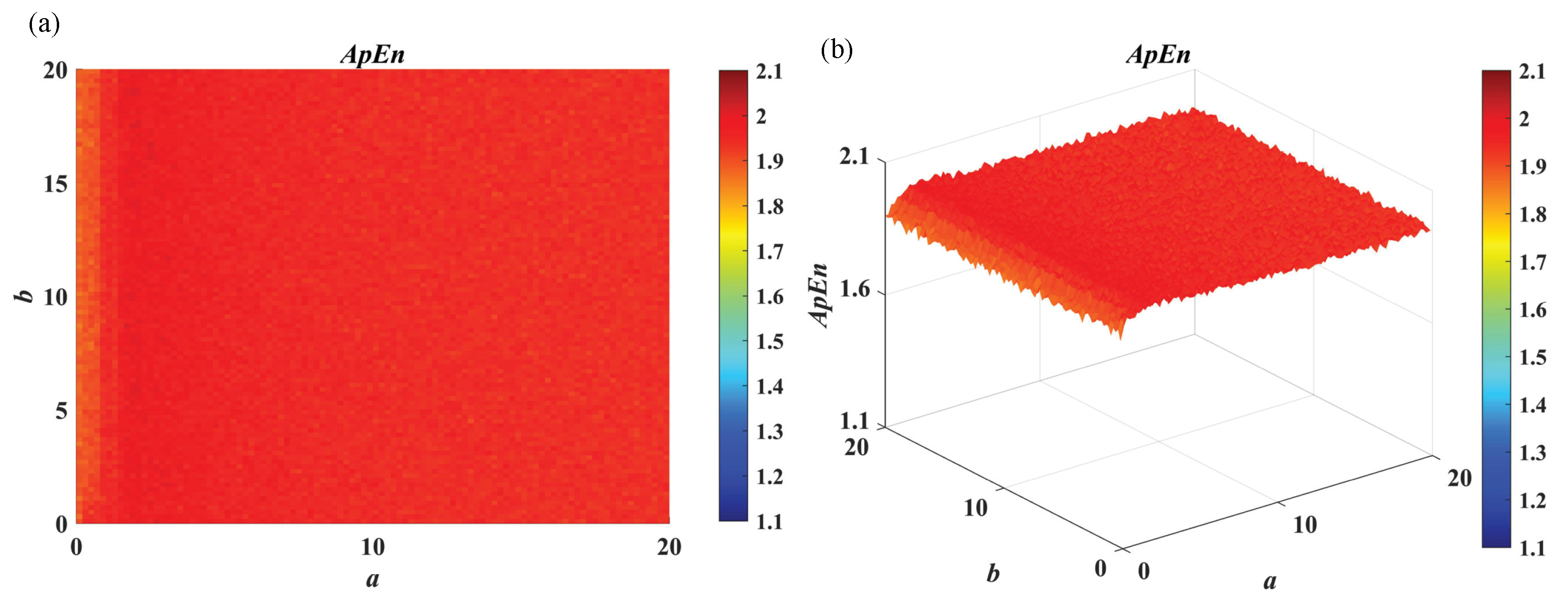
In the application of cryptography, the better the randomness of the chaotic time series, the higher the security of the cryptographic system. This paper uses approximate entropy (ApEn) [41] to test the complexity of the chaotic sequence of the system.
The ApEn complexity graph is used to measure the complexity of the system sequence, as Figure 6 shows. The color bars in Figure 6 represent the ApEn complexity value for x sequence of the 3D-SCC with corresponding parameters. The red region corresponds to higher complexity. The ApEn values are all greater than 1.8907, and the highest is 2.0411. The ApEn values are relatively stable, with a large area of red distributed on the top layer, indicating that the AE values are maintained at a high value and only fluctuate in a small range. Overall, the 3D-SCC map can output highly complex sequences within a wide range of parameters.
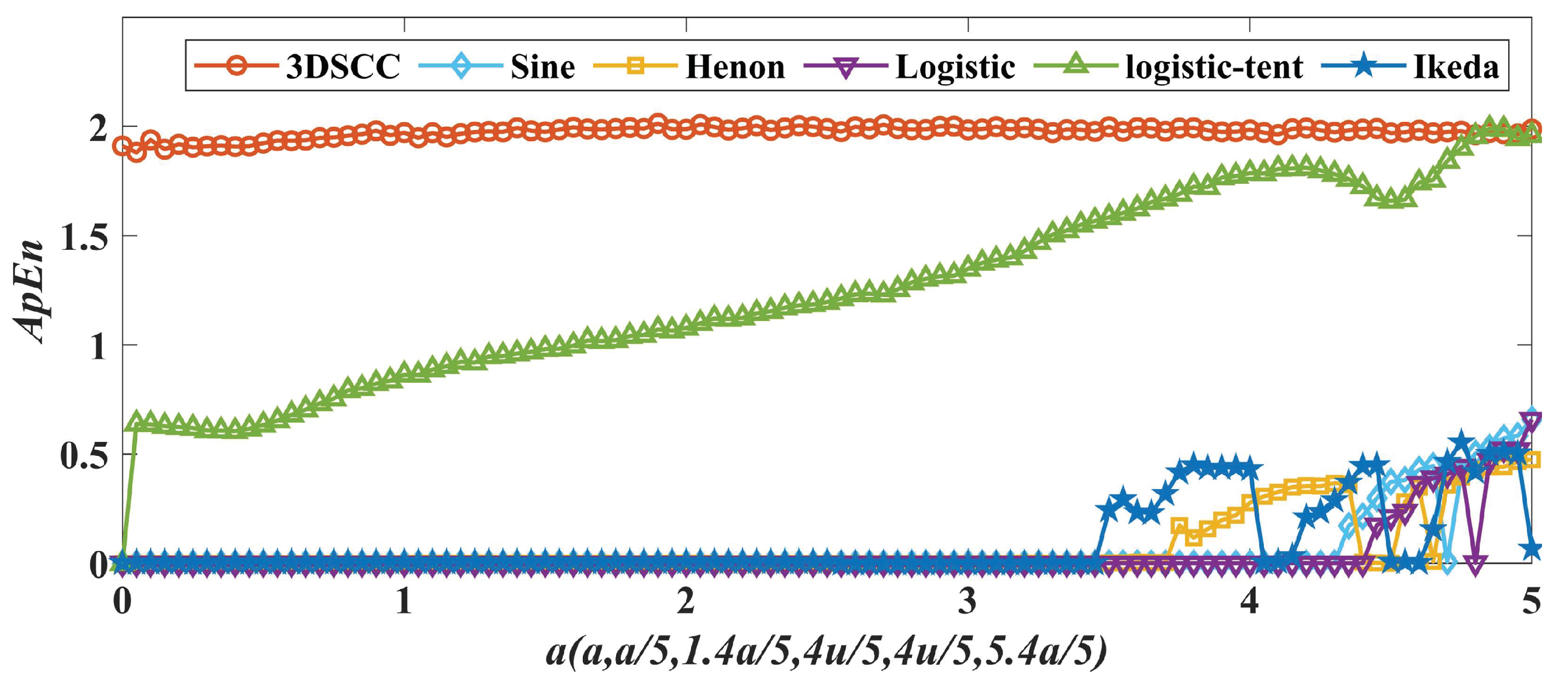
Figure 7 calculates the approximate entropy of other discrete chaos maps and compares them with the proposed map. It can be seen from Figure 6 that the AE values of the 3D-SCC are the largest within the parameter range, and all are stable at [1.893, 2.013]. Compared with other discrete chaotic sequences, the 3D-SCC system has high complexity with a wide parameter range. To summarize, this map is an excellent pseudo-random password generator, which is very suitable for the field of communication security.
3. Design of the Image Encryption Based on the Novel Discrete Hyperchaotic Map
This section proposes an image encryption based on the novel discrete hyperchaotic map, an image-sensitive function based on convolution and a dynamic cycle shift scramble algorithm. We explain the image-sensitive function and the dynamic cycle shift scramble algorithm and give detailed steps of the encryption algorithm below. Figure 8 shows the encryption algorithm flowchart.
3.1. Image-Sensitive Function Based on Convolution
The image sensitivity function is a function that is highly sensitive to image information. Even if the information of two images is slightly different, the output value is also completely different. This paper proposes an image-sensitive function based on a convolution operation to extract features. The calculation of the feature matrix uses each pixel value, the mean of all pixels value and the standard deviation of all pixels of the image, which is highly sensitive to the image.
The processed mean value and the processed standard deviation as initial values and parameters are input into the Sin-Tent chaos system to generate a chaotic sequence, and this sequence is used to construct a matrix as a convolution kernel. Then, the convolution kernel is used to perform a two-dimensional discrete convolution operation with the image to obtain an image feature matrix.
Sin-Tent chaos is defined as follows [34].
Suppose the image is , and the specific steps of extracting features are as follows.
Step 1 Calculate the parameter r and the initial value as follows:
where is the function calculating the standard deviation of data, and is the function calculating the mean of the data.
Step 2 The parameter r and the initial value are input into Sin-Tent chaos, and a chaotic sequence of length is obtained, as Equation (7) shows. The chaotic sequence is constructed into a matrix of as the convolution kernel .
Step 3 The horizontal sliding step length of the convolution operation is , and the vertical sliding step length is . Namely, the image is divided into non-overlapping blocks. The convolution kernel W performs convolution operation with each block; finally, a feature matrix S of is obtained, as Equation (9) shows. is the image block in the -th row and -th column of the image P.
3.2. Dynamic Cycle Shift Scramble Algorithm
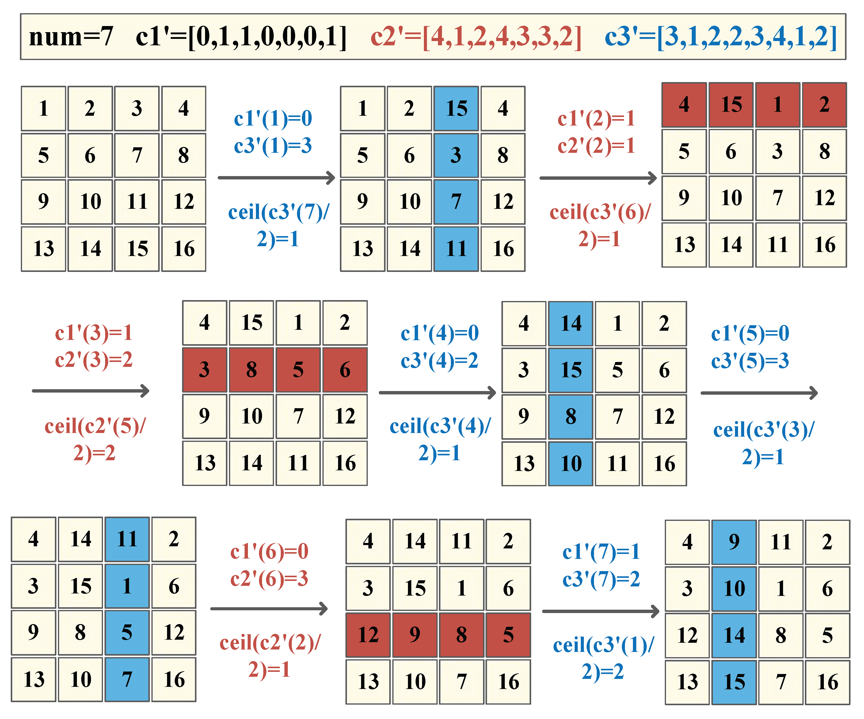
This section proposes a dynamic cycle shift scramble algorithm. The algorithm uses chaotic sequences to select the scrambling parameters for each time. The scrambling parameters include selecting a row or column, the number of rows/columns, and the cyclic shift step. Suppose the image to be scrambled is P. The size is . The total times of shifts are . The chaotic sequences are and their length are . Figure 9 shows an example of the algorithm.The specific algorithm steps are as follows. The algorithm program is shown in Algorithm 1. (-) means circulating the one-dimensional vector a to the left by n bits; is the round-up function.
Step 1 Use Equation (6) to process the chaotic sequence :
where is the modulus function, and is a function that rounds to positive infinity, and Set .
Step 2 If , select column scrambling and go to Step4. Otherwise, select the row scrambling and go to Step5.
Step 3 Select the column and perform the cyclic shift on this column with a step size of .
Step 4 Select the row and perform the cyclic shift on this row with a step size of .
Step 5 If , the algorithm ends. Otherwise, , go to Step2.
| Algorithm 1: Dynamic cycle shift scramble algorithm. |
| Procedure DCS() |
| Input: image P, chaos sequences |
| Output: Scrambled image |
| 1: |
| 2: |
| 3: |
| % (the sequence of selecting scrambled rows or columns) |
| 4: |
| % (the sequence of selecting the scrambling step size) |
| 5: |
| % (the sequence of selecting the scrambling step size) |
| 6: for i = 1 to |
| 7: if |
| 8: |
| % (Select the column and cyclically shift bits) |
| 9: else |
| 10: |
| % (Select the column and cyclically shift bits) |
| 11: end if |
| 12: end for |
3.3. Image Encryption Steps
Using the hyperchaotic map 3D-SCC, this section proposes an image encryption algorithm based on the dynamic cycle shift scramble algorithm, the image-sensitive function and the integer wavelet transform. Suppose the plaintext image is , the gray image, and the specific encryption steps are as follows. If the plaintext image is a colour image, each of the three channels will be encrypted using the following algorithm, and then the ciphertexts of the three channels will be combined into the ciphertext of the plaintext image.
Step 1 According to the steps in Section 2.2, setting = 8 and (if M is not a multiple of 8, and N is not a multiple of 2, the condition can be achieved by adding 0), generating the feature matrix of the plaintext image. is the key, and we set the private key .
Step 2 Calculate as follows:
Step 3 Perform integer haar wavelet transform on the plaintext image to obtain the low-frequency part , and the high-frequency parts . Only encrypt by using and the dynamic cycle shift scramble algorithm to obtain the scrambled low-frequency part . The algorithm programs are shown in Algorithms 2 and 3.
| Algorithm 2: 3D-SCC. |
| Procedure 3D-SCC () |
| Input: the parameters the initial value the length of sequence m. |
| Output: sequences |
| 1: |
| 2: |
| 3: |
| 4: for i = 2 to m |
| 5: |
| 6: |
| 7: |
| 8: end for |
| Algorithm 3: Scrambling part. |
| Input: . |
| Output: the scrambled part |
| 1: |
| % (According to algorithm 2) |
| 2: |
| % (According to algorithm 1) |
Step 4 Perform integer wavelet reconstruction on to obtain the semi-encrypted image .
Step 5 Input into the 3D-SCC chaos map and process the obtained chaotic sequence into a chaotic matrix. The semi-encrypted image is divided into four non-overlapping image blocks. Four different chaotic matrices are used to perform bitwise XOR operations with the four image blocks, respectively, to obtain the final ciphertext image . The algorithm program is shown in Algorithm 4.
| Algorithm 4: Diffusion part. |
| Input: the semi-encrypted image . |
| Onput: the final encrypted image . |
| 1: |
| 2: |
| 3: |
| 4: |
| 5: |
| 6: |
| 7: |
| 8: |
| 9: |
| 10: |
4. Simulation Experiments
To test the effectiveness of the algorithm, this paper used the USC-SIPI[dataset] images dataset and Lena image (512 × 512) for experimentation. The following will make a statistical analysis, an anti-differential attack test and an anti-attack test on the ciphertext to illustrate the security of the ciphertext. This paper used MATLAB 2020a to conduct simulation experiment on a personal computer with an Inter(R) Core(TM) i5-1035G1 CPU @ 3.60 GHz and 16.00 GB memory, and the operating system was a Microsoft Windows 10.
4.1. Ciphertext of Scrambling Algorithm
The traditional scrambling algorithm by chaotic sequence is to process the chaotic sequence in ascending or descending order to obtain a chaotic subscript sequence and use the subscript sequence to scramble the rows or columns of the image. The ciphertext obtained by this algorithm has obvious horizontal stripes, vertical stripes or lattice textures, which can be easily deciphered, as shown in Figure 10a–c. Based on this problem, we propose a dynamic scrambling algorithm that alternately scrambles between rows and columns. The ciphertext after scrambling is shown in Figure 10d, and no texture can be seen, which is better than traditional algorithms.
4.2. Histogram
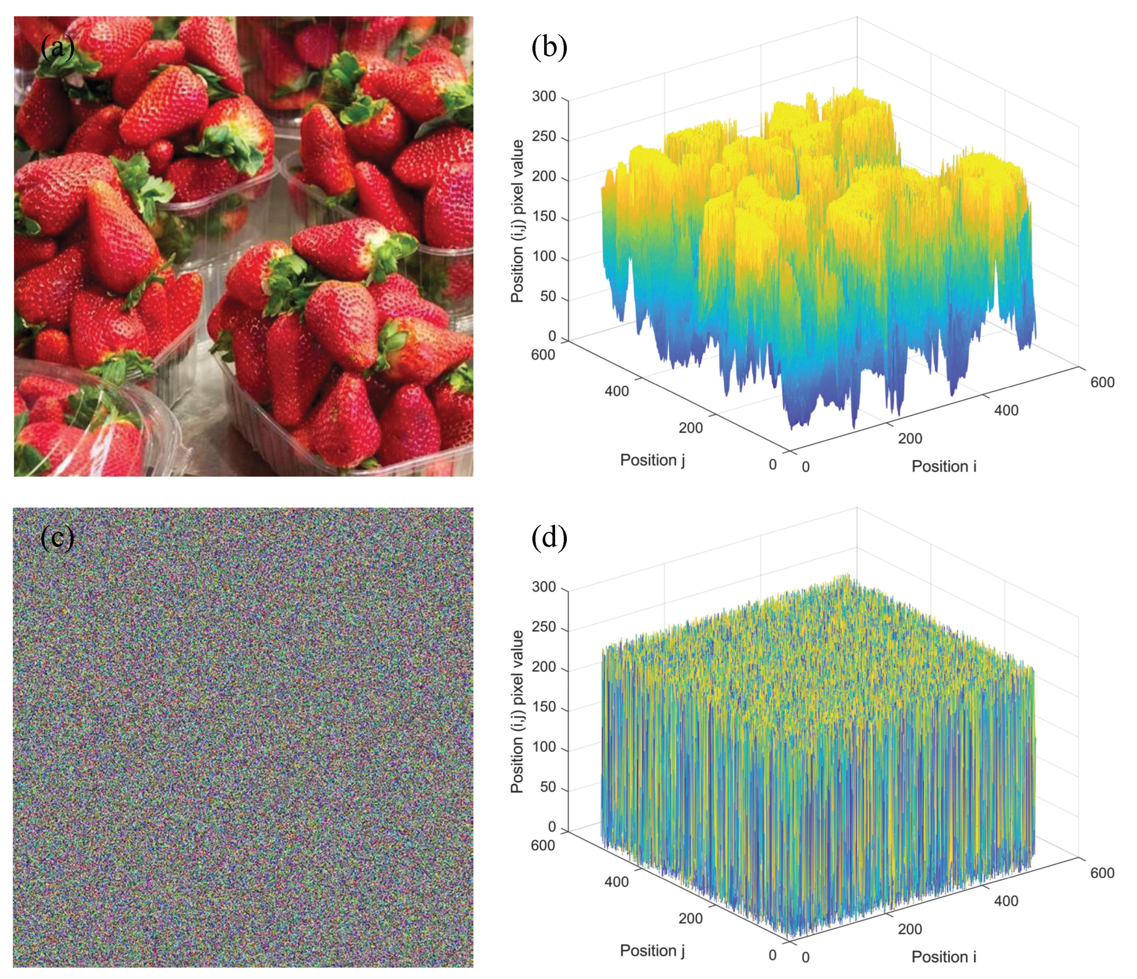
The histogram is an important statistical characteristic of the image. The 3D histogram describes the gray level of each position of the image, including both the gray level numerical information and the position information. Figure 11, Figure 12 and Figure 13 show the plaintexts, corresponding ciphertexts and their histograms. They include gray and color, square and rectangle images. The plaintext types include grayscale and colour maps, and sizes include rectangular and square, which illustrate the flexibility of the algorithm. It can be seen that the plaintext histograms have obvious statistical characteristics, while the ciphertexts conceal the statistical characteristics of the plaintexts, which verify the effectiveness of the encryption algorithm.
4.3. Correlation Coefficient of Adjacent Pixels
The correlation of adjacent pixels is one of the important characteristics of an image. In plaintext images, neighboring pixels have a high correlation. An effective encrypted image should generate ciphertext with a low correlation between adjacent pixels. The correlation of adjacent pixels in the three directions of the ciphertext is shown in Table 1. Bolded datas in the table indicate better results. It can be seen that the correlation coefficients of adjacent pixels are all close to 0, which eliminates the statistical characteristics of the plaintext. Compared with other schemes, the correlation between adjacent pixels of the ciphertext of our algorithm is closer to 0. In Figure 14, most of the adjacent pixels of the plaintext are concentrated on the diagonal, which shows that the adjacent pixels of the plaintext are relatively correlated. The adjacent pixels of the ciphertext are evenly distributed, and there is no statistical law, which verifies the effectiveness of the encryption algorithm.
4.4. Information Entropy
Information entropy reflects the amount of information contained in an image and is a statistical form of image features. The Shannon entropy [10] is calculated as follows.
where m is the image, and is the probability of gray value in the image. The ideal value of the Shannon entropy for the 256 gray level image is 8. Recently, Wu et al. proposed the local Shannon entropy(LoSE) to fairly evaluate the randomness [43]. For an image m, it randomly chooses k non-overlapping image blocks with pixels in the image P, and LoSE is calculated as follows:
According to [43], the LoSE is better to fall in the interval . Let and . Table 2 shows LoSEs of cipher images encrypted by different schemes. Bolded datas in the table indicate better results. Compared with other algorithms, our scheme has the highest pass rate, the highest mean value and the lowest standard deviation, which indicates the cipher images encrypted by our scheme are random-like.
4.5. Anti-Differential Attack
The differential attack is to use the same encryption algorithm to encrypt the plaintext images before and after the change by making small changes to the plaintext image and to compare the encrypted results to achieve the purpose of deciphering the algorithm. The number of pixels changes rate (NPCR) and the number average changing intensity (UACI) are used to evaluate the sensitivity of the ciphertext image of the algorithm to the plaintext image [46]. The calculation formulas of NPCR and UACI are shown in Equations (14) and (15).
where and are two ciphertext images encrypted with only slightly different images.
In [46], Wu et al. proposed a statistical hypothesis of NPCR and UACI. We set and the and of different sizes image as shown in Table 3. We used 25 grayscale images from the USC-SIPI database for experiments. We randomly modified a pixel value and calculated the NPCR and UACI. In addition, each image was tested 100 times. The results are shown in Figure 15. Table 4 and Table 5 show the NPCR and UACI results of different schemes. Bolded datas in the table indicate better results. It can be observed that the scheme of this paper has a high pass rate and is closer to the ideal value than other schemes, which indicates our scheme exhibits resistance against differential attacks.
4.6. Rubust Test
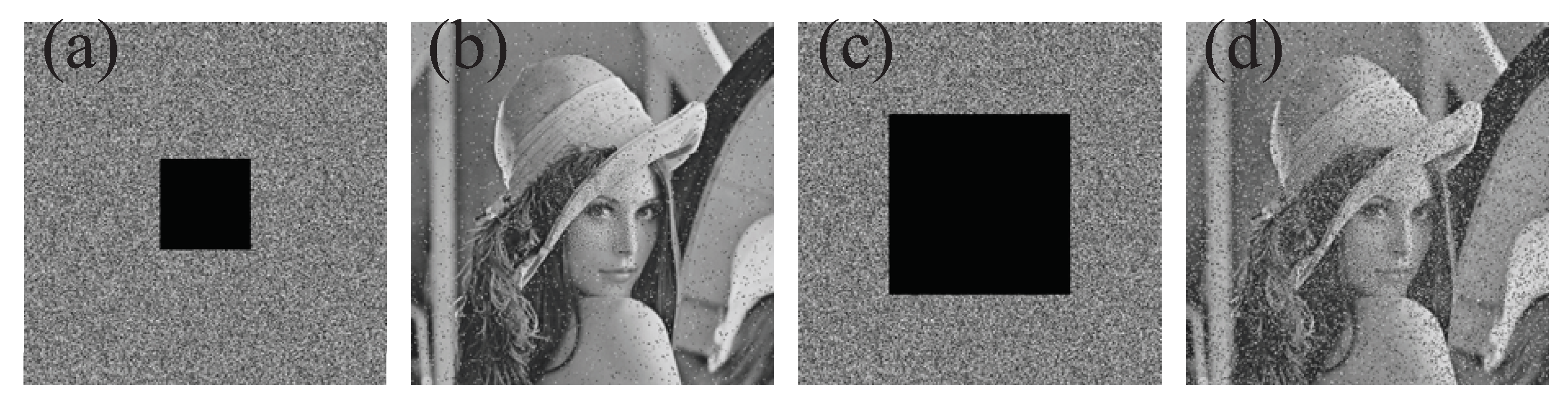
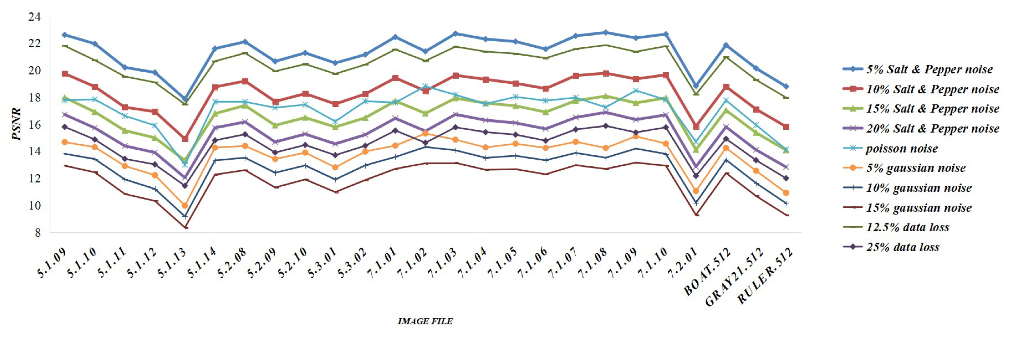
The attacked ciphertext image was decrypted to test the anti-attack of the algorithm. The ciphertext images were attacked by cutting 12.5%, 25%, add 5%, 10%, 15%, 20% Salt and Pepper noise, add 5%, 10%, 15% Gaussian noise and Poisson noise, respectively. The ciphertext images after the cropping attack and the corresponding decrypted images are shown in Figure 16. The ciphertext images after noise attack and the corresponding decrypted images are shown in Figure 17. Although the decrypted image is slightly noisy, the content is clear and identifiable, which shows that the algorithm has a certain degree of resistance to attack. The peak signal-to-noise ratio (PSNR) is used to measure the quality of the decrypted image, and the calculation formula of PSNR is shown in Equation (16). The higher the value of PSNR is, the smaller the degree of distortion. The PSNR value of the decrypted image is shown in Figure 18. As can be observed, the PSNR value of Salt and Pepper noise attack is bigger than that of the Gaussian noise attack, which means the encryption algorithms are more resistant to Salt and Pepper noise attacks. It can be concluded that the proposed algorithm has a strong ability to resist noise and cropping attacks.
4.7. Key Space
The key space is the number of possibilities for all combinations of encryption system keys, which is determined by the length of the key. When the key is the decimal bit, the precision is 15 and the length is . There are kinds of key combination possibilities, i.e., the size of the key space is . From the relationship between key space and key length, the longer the key length, the larger the key space. The longer the key length is, the larger the key space. In theory, the longer the key length of the encryption system, the more secure the encryption system is, but in reality, it is impossible to set an infinite key length, i.e., it is impossible to have infinite key space, and in fact, there is no need for infinite key space. The literature [48] suggests that when the key space is greater than , the key can effectively resist exhaustive attacks. The key space of this paper is , or , which is sufficient to resist brute force and exhaustive attacks. In terms of the key space of the system alone, the algorithm proposed in this paper has good security performance.
4.8. Known and Chosen Plaintext Attack
The known plaintext attack is a mode of attack in which the attacker owns a piece of plaintext and the corresponding ciphertext. The goal of the attacker is to construct an equivalent decryption algorithm or derive an equivalent key for the cryptograph to crack the entire ciphertext [49]. Selective plaintext attacks are performed by constructing a special plaintext image and inputting it into encryption algorithms, using ciphertext pairs and a deciphering algorithm to obtain an equivalent key [49].
For a linear encryption system, the encryption system can be easily broken when an attacker uses a known or chosen plaintext attack on the encryption system. In the encryption algorithm proposed in this paper, the key is strongly correlated with the size and pixel value of the plaintext. In addition, the encryption methods used in this paper for confusion in the wavelet domain and diffusion using xor operation are both non-linear processes, making it difficult for an attacker to obtain the correct key. A plaintext image with all 0 pixels is fed into the encryption algorithm, and the corresponding ciphertext is a snowflake image with no statistical features. When an attacker adopts a chosen plaintext attack on the image encryption algorithm based on integer haar wavelet transform and dynamic confusion, he will undoubtedly only obtain a disorganized image and will not be able to obtain the original image information from the image. Thus, the proposed image encryption algorithm based on integer haar wavelet transform and dynamic scramble can withstand both known plaintext attacks and chosen plaintext attacks.
5. Conclusions
This paper proposes a novel wide-range discrete hyperchaotic map (3D-SCC), the mathematical model of the Sine map, which is based on one sine function and two cosine functions. Through trajectory analysis, the Lyapunov exponent spectrum and approximate entropy analysis, we verified that the proposed map is in the hyperchaotic state with a wide range of parameters, has enough complex sequences and good ergodicity. To improve the security of the encryption algorithm, we designed an image-sensitive function based on convolution to better resist differential attacks and the dynamic cycle shift scrambling algorithm to better scramble. In addition, we performed integer wavelet transform on the plaintext and only scrambled the low-frequency part to improve computational efficiency. Simulated experiments show that the algorithm has excellent performances against attacks, in particular statistical attacks, differential attacks, cut attacks and noisy attacks. The algorithm in this paper is safe, efficient and anti-attack and has practical application value.
Author Contributions
H.Z. wrote the manuscript; H.Z., G.L., X.X. and X.S. performed the literature review; and H.Z. submitted the manuscript to the journal. All authors have read and agreed to the published version of the manuscript.
Funding
This research was funded by Natural Science Foundation of Guangxi province of Guodong Li No. 2022gxnsfaa035554, Guilin University of Electronic Technology Fund of Guodong Li grant number No. C21YJM00QX99, the Innovation Project of GUET Graduate Education of Huiyan Zhong grant number No. 2022YCX139 and supported by the Key Laboratory of Data Analysis and Computation in Universities in Guangxi Autonomous Region and the Guangxi Center for Applied Mathematics (Guilin University of Electronic Science and Technology).
Institutional Review Board Statement
Not applicable.
Informed Consent Statement
Not applicable.
Data Availability Statement
Not applicable.
Conflicts of Interest
The authors declare that this research was conducted in the absence of any commercial or financial relationships that may be construed as a potential conflict of interest.
References
- Sagde, R.Z.; Usikov, D.; Zaslavsky, G.; Wilson, M.K. Nonlinear Physics: From the Pendulum to Turbulence and Chaos. Appl. Opt. 1988, 42, 4. [Google Scholar]
- Fan, C.; Ding, Q. A universal method for constructing non-degenerate hyperchaotic systems with any desired number of positive Lyapunov exponents. Chaos Solitons Fractals 2022, 161, 112323. [Google Scholar] [CrossRef]
- Wolf, A.; Swift, J.; Swinney, H.L.; Vastano, J.A. Determining Lyapunov exponents from a time series. Phys. Nonlinear Phenom. 1985, 16, 285–317. [Google Scholar] [CrossRef] [Green Version]
- Gupta, M.D.; Chauhan, R.K. Secure image encryption scheme using 4D-Hyperchaotic systems based reconfigurable pseudo-random number generator and S-Box. Integration 2021, 81, 137–159. [Google Scholar] [CrossRef]
- Griffin, J. The Sine Map. 2013. Available online: https://0-people-maths-bris-ac-uk.brum.beds.ac.uk/~macpd/ads/sine.pdf (accessed on 10 April 2022).
- Jafari, S.; Pham, V.T.; Golpayegani, S.M.R.H.; Moghtadaei, M.; Kingni, S.T. The Relationship Between Chaotic Maps and Some Chaotic Systems with Hidden Attractors. Int. J. Bifurc. Chaos 2016, 26, 1650211:1–1650211:8. [Google Scholar] [CrossRef]
- Chua, L.O.; Itoh, M.; Kocarev, L.; Eckert, K. Chaos Synchronization in Chua’s Circuit. J. Circuits Syst. Comput. 1993, 3, 93–108. [Google Scholar] [CrossRef]
- Hénon, M. A two-dimensional mapping with a strange attractor. Commun. Math. Phys. 1976, 50, 69–77. [Google Scholar] [CrossRef]
- Sprott, J.C. Chaos and Time-Series Analysis; Oxford University Press: Oxford, UK, 2003. [Google Scholar]
- Shannon, C.E. Communication theory of secrecy systems. Bell Syst. Tech. J. 1949, 28, 656–715. [Google Scholar] [CrossRef]
- Lorenz, E.N. Deterministic nonperiodic flow. J. Atmos. Sci. 1963, 20, 130–141. [Google Scholar] [CrossRef] [Green Version]
- Hua, Z.; Zhou, Y.; Pun, C.M.; Chen, C. 2D Sine Logistic modulation map for image encryption. Inf. Sci. 2015, 297, 80–94. [Google Scholar] [CrossRef]
- Gholamin, P.; Sheikhani, A.H.R. A new three-dimensional chaotic system: Dynamical properties and simulation. Chin. J. Phys. 2017, 55, 1300–1309. [Google Scholar] [CrossRef]
- Zhao, H.; Xie, S.; Zhang, J.; Wu, T. A dynamic block image encryption using variable-length secret key and modified Henon map. Optik 2021, 230, 166307. [Google Scholar] [CrossRef]
- Zhong, H.; Li, G. Multi-image encryption algorithm based on wavelet transform and 3D shuffling scrambling. Multim. Tools Appl. 2022, 81, 24757–24776. [Google Scholar] [CrossRef]
- Hassaballah, M. 1—Introduction to digital image steganography. In Digital Media Steganography; Academic Press: Cambridge, MA, USA, 2020; pp. 1–15. [Google Scholar]
- Kadhim, I.J.; Premaratne, P.; Vial, P.J.; Halloran, B. Comprehensive survey of image steganography: Techniques, Evaluations, and trends in future research. Neurocomputing 2019, 335, 299–326. [Google Scholar] [CrossRef]
- Jose, A.; Subramaniam, K. DNA based SHA512-ECC cryptography and CM-CSA based steganography for data security. Mater. Today Proc. 2020. [Google Scholar] [CrossRef]
- Mahto, D.K.; Singh, A. A survey of color image watermarking: State-of-the-art and research directions. Comput. Electr. Eng. 2021, 93, 107255. [Google Scholar] [CrossRef]
- Evsutin, O.; Melman, A.; Meshcheryakov, R. Digital Steganography and Watermarking for Digital Images: A Review of Current Research Directions. IEEE Access 2020, 8, 166589–166611. [Google Scholar] [CrossRef]
- Singh, O.P.; Singh, A.K.; Srivastava, G.; Kumar, N. Image watermarking using soft computing techniques: A comprehensive survey. Multim. Tools Appl. 2021, 80, 30367–30398. [Google Scholar] [CrossRef]
- Midoun, M.A.; Wang, X.; Talhaoui, M.Z. A sensitive dynamic mutual encryption system based on a new 1D chaotic map. Opt. Lasers Eng. 2021, 139, 106485. [Google Scholar] [CrossRef]
- Li, G.D.; Wang, L.-I. Double chaotic image encryption algorithm based on optimal sequence solution and fractional transform. Vis. Comput. 2019, 35, 1267–1277. [Google Scholar] [CrossRef]
- Li, G.D.; Zhao, G.M.; Xu, W.X.; Yao, S. Research on Application of Image Encryption Technology Based on Chaotic of Cellular Neural Network. J. Digit. Inf. Manag. 2014, 12, 151–158. [Google Scholar]
- Rasul Enayatifar, F.G.G.; Siarry, P. Index-based permutation-diffusion in multiple-image encryption using DNA sequence. Opt. Lasers Eng. 2019, 115, 131–140. [Google Scholar] [CrossRef]
- Lu, Q.; Zhu, C.; Deng, X. An Efficient Image Encryption Scheme Based on the LSS Chaotic Map and Single S Box. IEEE Access 2020, 8, 25664–25678. [Google Scholar] [CrossRef]
- Alawida, M.; Samsudin, A.; Teh, J.S.; Alkhawaldeh, R.S. A new hybrid digital chaotic system with applications in image encryption. Signal Process. 2019, 160, 45–58. [Google Scholar] [CrossRef]
- Farah, M.A.B.; Guesmi, R.; Kachouri, A.; Samet, M. A novel chaos based optical image encryption using fractional Fourier transform and DNA sequence operation. Opt. Laser Technol. 2020, 121, 105777. [Google Scholar] [CrossRef]
- Zhu, S.; Wang, G.; Zhu, C. A Secure and Fast Image Encryption Scheme Based on Double Chaotic S-Boxes. Entropy 2019, 21, 790. [Google Scholar] [CrossRef] [Green Version]
- Huang, Z.; Cheng, S.; Gong, L.; Zhou, N. Nonlinear optical multi-image encryption scheme with two-dimensional linear canonical transform. Opt. Lasers Eng. 2020, 124, 105821. [Google Scholar] [CrossRef]
- Jiang, X.; Xiao, Y.; Xie, Y.; Liu, B.; Ye, Y.; Song, T.; Chai, J.; Liu, Y. Exploiting optical chaos for double images encryption with compressive sensing and double random phase encoding. Opt. Commun. 2021, 484, 126683. [Google Scholar] [CrossRef]
- Matthews, R. On the Derivation of a ’Chaotic’ Encryption Algorithm. Cryptologia 1989, 13, 29–42. [Google Scholar] [CrossRef]
- Zhou, Y.; Bao, L.; Chen, C.L.P. A new 1D chaotic system for image encryption. Signal Process. 2014, 97, 172–182. [Google Scholar] [CrossRef]
- Farah, M.A.B.; Farah, A.; Farah, T. An image encryption scheme based on a new hybrid chaotic map and optimized substitution box. Nonlinear Dyn. 2019, 99, 3041–3064. [Google Scholar] [CrossRef]
- Hua, Z.; Zhou, Y.; Huang, H. Cosine-transform-based chaotic system for image encryption. Inf. Sci. 2019, 480, 403–419. [Google Scholar] [CrossRef]
- An, F.; Liu, J.E. Image Encryption Algorithm Based on Adaptive Wavelet Chaos. J. Sens. 2019, 2019, 2768121. [Google Scholar] [CrossRef]
- Shakir, H.R. An image encryption method based on selective AES coding of wavelet transform and chaotic pixel shuffling. Multimed. Tools Appl. 2019, 78, 26073–26087. [Google Scholar] [CrossRef]
- Huo, D.; Zhu, Z.; Wei, L.; Han, C.; Zhou, X. A visually secure image encryption scheme based on 2D compressive sensing and integer wavelet transform embedding. Opt. Commun. 2021, 492, 126976. [Google Scholar] [CrossRef]
- Gao, X. Hidden attractors in dynamical systems. Opt. Laser Technol. 2021, 142, 107252. [Google Scholar] [CrossRef]
- Lai, D.; Chen, G. Statistical analysis of Lyapunov exponents from time series: A Jacobian approach. Math. Comput. Model. 1998, 27, 1–9. [Google Scholar] [CrossRef]
- Pincus, S.M. Approximate entropy as a measure of system complexity. Proc. Natl. Acad. Sci. USA 1991, 88, 2297–2301. [Google Scholar] [CrossRef] [Green Version]
- Mansouri, A.; Wang, X. A novel one-dimensional sine powered chaotic map and its application in a new image encryption scheme. Inf. Sci. 2020, 520, 46–62. [Google Scholar] [CrossRef]
- Wu, Y.; Zhou, Y.; Saveriades, G.; Agaian, S.S.; Noonan, J.P.; Natarajan, P. Local Shannon entropy measure with statistical tests for image randomness. Inf. Sci. 2013, 222, 323–342. [Google Scholar] [CrossRef] [Green Version]
- Mansouri, A.; Wang, X. A novel one-dimensional chaotic map generator and its application in a new index representation-based image encryption scheme. Inf. Sci. 2021, 563, 91–110. [Google Scholar] [CrossRef]
- Talhaoui, M.Z.; Wang, X. A new fractional one dimensional chaotic map and its application in high-speed image encryption. Inf. Sci. 2021, 550, 13–26. [Google Scholar] [CrossRef]
- Wu, Y.; Noonan, J.P.; Agaian, S.S. NPCR and UACI Randomness Tests for Image Encryption. Cyber J. Multidiscip. J. Sci. Technol. J. Sel. Areas Telecommun. (JSAT) 2011, 2, 31–38. [Google Scholar]
- Hua, Z.; Jin, F.; Xu, B.; Huang, H. 2D Logistic-Sine-coupling map for image encryption. Signal Process. 2018, 149, 148–161. [Google Scholar] [CrossRef]
- Zhang, Y.; Li, C.; Li, Q.; Zhang, D.; Shu, S. Breaking a chaotic image encryption algorithm based on perceptron model. Nonlinear Dyn. 2011, 69, 1091–1096. [Google Scholar] [CrossRef]
- Pace, D.K. The Codebreakers: The Comprehensive History of Secret Communication from Ancient Times to the Internet. Naval War Coll. Rev. 1998, 51, 4. [Google Scholar]
Figure 1.
Phase diagrams. with and . (a) x-y-z plane; (b) x-y plane; (c) z-y plane; (d) x-z plane.

Figure 2.
Histogram: (a) 3D-SCC with and ; (b) the Sine map with and .

Figure 3.
Dynamics of the Sine map: (a) Lyapunv exponent spectrum with different s (the control parameter) and ; (b) bifurcation diagram with different s (the control parameter) and .
Figure 3.
Dynamics of the Sine map: (a) Lyapunv exponent spectrum with different s (the control parameter) and ; (b) bifurcation diagram with different s (the control parameter) and .

Figure 4.
Dynamics of the 3D-SCC: (a,d) LEs and BD with and ; (b,e) LEs and BD with and ; (c,f) LEs and BD with and .
Figure 4.
Dynamics of the 3D-SCC: (a,d) LEs and BD with and ; (b,e) LEs and BD with and ; (c,f) LEs and BD with and .

Figure 5.
Dynamics of the 3D-SCC. (a,d) LEs and BD with and , , ; (b,e) LEs and BD with and ; (c,f) LEs and BD with and .
Figure 5.
Dynamics of the 3D-SCC. (a,d) LEs and BD with and , , ; (b,e) LEs and BD with and ; (c,f) LEs and BD with and .

Figure 6.
ApEn complexity graph. The 3D-SCC with and . (a) a-b plane; (b) space diagram.

Figure 7.
Approximate entropy comparison with a different chaos system. The 3D-SCC (, , ), the Sine map (, ), the Henon map ( , ), the logistic map (,), the logistic-tent (, ), the Ikeda map ( ) for .
Figure 7.
Approximate entropy comparison with a different chaos system. The 3D-SCC (, , ), the Sine map (, ), the Henon map ( , ), the logistic map (,), the logistic-tent (, ), the Ikeda map ( ) for .

Figure 8.
Encryption algorithm flowchart.

Figure 9.
Examples of scrambling algorithms.

Figure 10.
Scrambling algorithm ciphertext image: (a) row scrambling only; (b) column scrambling only; (c) scrambling rows and columns in order; (d) scrambling algorithm.
Figure 10.
Scrambling algorithm ciphertext image: (a) row scrambling only; (b) column scrambling only; (c) scrambling rows and columns in order; (d) scrambling algorithm.

Figure 11.
(a) Lena (512 × 512, Gray); (b) histograms of Lena; (c) ciphertext of Lena; (d) histograms of ciphertext.
Figure 11.
(a) Lena (512 × 512, Gray); (b) histograms of Lena; (c) ciphertext of Lena; (d) histograms of ciphertext.

Figure 12.
(a) Black (512 × 1024, Gray); (b) histograms of Black; (c) ciphertext of Lena; (d) histograms of ciphertext.
Figure 12.
(a) Black (512 × 1024, Gray); (b) histograms of Black; (c) ciphertext of Lena; (d) histograms of ciphertext.

Figure 13.
(a) Strawberries (512 × 512, RGB); (b) histograms of strawberries; (c) ciphertext of strawberries; (d) histograms of ciphertext.
Figure 13.
(a) Strawberries (512 × 512, RGB); (b) histograms of strawberries; (c) ciphertext of strawberries; (d) histograms of ciphertext.

Figure 14.
Adjacent pixels in the horizontal, vertical and diagonal direction of plaintext and ciphertext: (a–c) Lena; (d–f) the ciphertext of Lena; (g–i) all-black; (j–l) the ciphertext of All-black; (m–o) 4.2.03.tiff; (p–r) the ciphertext 4.2.03.tiff. The red, green and blue shops correspond to the three channels of the colour image.

Figure 15.
NPCR and UACI results: (a) NPCR results of 25 images from USC-SIPI dataset; (b) UACI results of 25 images from USC-SIPI dataset.
Figure 15.
NPCR and UACI results: (a) NPCR results of 25 images from USC-SIPI dataset; (b) UACI results of 25 images from USC-SIPI dataset.

Figure 16.
Ciphertext images after cutting attack and corresponding decrypted images: (a,b) cut 12.5%; (c,d) cut 25%.
Figure 16.
Ciphertext images after cutting attack and corresponding decrypted images: (a,b) cut 12.5%; (c,d) cut 25%.

Figure 17.
Ciphertext images after noise attack and corresponding decrypted images.: (a,b) 5% Salt and Pepper noise; (c,d) 10% Salt and Pepper noise; (e,f) 15% Salt and Pepper noise; (g,h) 20% Salt and Pepper noise; (i,j) Poisson noise; (k,l) 5% Guassian noise; (m,n) adding 10% Guassian noise; (o,p) 20% Guassian noise.

Figure 18.
PSNR of the decrypted image of attacked ciphertext image.


Table 1.
Correlation coefficients of cipher images by other scheme.
| Image | Scheme | Horizontal | Vertical | Diagonal | Average |
|---|---|---|---|---|---|
| Lena | this paper | 0.001348 | 0.00016 | 0.002236 | 0.001248000 |
| [42] | −0.00205 | −0.00509 | −0.00398 | 0.003706667 | |
| 5.1.12 | this paper | 0.000357 | −0.000128 | −0.00374 | 0.001407667 |
| [42] | 0.00224 | −0.00209 | 0.00102 | 0.001783333 | |
| boat.512 | this paper | 0.001582 | 0.000183 | 0.000286 | 0.000683667 |
| [42] | −0.00019 | −0.00329 | −0.000044 | 0.001174667 | |
| 5.3.01 | this paper | −0.00011 | −0.000036 | −0.001721 | 0.000622333 |
| [42] | −0.00037 | 0.00156 | 0.0000639 | 0.000664633 |
Table 2.
LoSEs of different cipher images encrypted by different schemes.
| Image | [44] | [22] | [45] | Our |
|---|---|---|---|---|
| 5.1.09 | 7.902572 | 7.902488 | 7.902967 | 7.903489 |
| 5.1.10 | 7.900289 | 7.901408 | 7.902436 | 7.903029 |
| 5.1.11 | 7.903740 | 7.904619 | 7.904837 | 7.906463 |
| 5.1.12 | 7.902851 | 7.900101 | 7.890333 | 7.90536 |
| 5.1.13 | 7.900933 | 7.902922 | 7.903234 | 7.902903 |
| 5.1.14 | 7.905610 | 7.902073 | 7.902911 | 7.90531 |
| 5.2.08 | 7.902309 | 7.902984 | 7.9035000 | 7.904298 |
| 5.2.09 | 7.904542 | 7.902610 | 7.902604 | 7.902574 |
| 5.2.10 | 7.901099 | 7.902295 | 7.902812 | 7.902946 |
| 5.3.01 | 7.903069 | 7.904512 | 7.902591 | 7.902073 |
| 5.3.02 | 7.902729 | 7.901861 | 7.902850 | 7.902474 |
| 7.1.01 | 7.903035 | 7.901204 | 7.903333 | 7.902694 |
| 7.1.02 | 7.902222 | 7.902573 | 7.901752 | 7.902734 |
| 7.1.03 | 7.902076 | 7.902113 | 7.904041 | 7.902889 |
| 7.1.04 | 7.901261 | 7.902004 | 7.901952 | 7.902316 |
| 7.1.05 | 7.902481 | 7.902155 | 7.902065 | 7.902303 |
| 7.1.06 | 7.902062 | 7.902419 | 7.902507 | 7.901997 |
| 7.1.07 | 7.902413 | 7.902489 | 7.902027 | 7.901730 |
| 7.1.08 | 7.902846 | 7.901884 | 7.902023 | 7.902573 |
| 7.1.09 | 7.905016 | 7.905070 | 7.902044 | 7.901978 |
| 7.1.10 | 7.902937 | 7.902061 | 7.902021 | 7.902089 |
| 7.2.01 | 7.902964 | 7.902284 | 7.902051 | 7.903141 |
| boat.512 | 7.905313 | 7.902848 | 7.902769 | 7.90236 |
| gray21.512 | 7.902398 | 7.902648 | 7.902200 | 7.902637 |
| ruler.512 | 7.898843 | 7.901700 | 7.902178 | 7.902199 |
| Pass/All | 14/25 | 16/25 | 18/25 | 18/25 |
| Mean | 7.902624363 | 7.902453 | 7.90216154 | 7.90298236 |
| Std | 0.001517617 | 0.001054775 | 0.002567945 | 0.001175332 |
Table 3.
The and of different sizes image.
| Size | ||
|---|---|---|
| 256 × 256 | 99.57% | [33.2824%, 33.6447%] |
| 512 × 512 | 99.59% | [33.3730%, 33.5541%] |
| 1028 × 1028 | 99.60% | [33.4183%, 33.5088%] |
Table 4.
NPCR of different cipher images encrypted by different schemes.
| NPCR (%) | [47] | [22] | [44] | Our | Pass Rate |
|---|---|---|---|---|---|
| 5.1.09 | 99.6064 | 99.7528 | 99.5975 | 99.6109 | 96 |
| 5.1.10 | 99.6154 | 99.8062 | 99.6184 | 99.6108 | 96 |
| 5.1.11 | 99.6244 | 99.7253 | 99.6064 | 99.6071 | 97 |
| 5.1.12 | 99.5703 | 99.7955 | 99.6661 | 99.6088 | 95 |
| 5.1.13 | 99.6109 | 99.7803 | 99.6005 | 99.6087 | 95 |
| 5.1.14 | 99.6364 | 99.8016 | 99.5915 | 99.6097 | 93 |
| 5.2.08 | 99.5870 | 99.8493 | 99.6128 | 99.6082 | 99 |
| 5.2.09 | 99.6260 | 99.8257 | 99.6022 | 99.6091 | 93 |
| 5.2.10 | 99.6124 | 99.7627 | 99.6271 | 99.6081 | 95 |
| 5.3.01 | 99.5931 | 99.8585 | 99.6012 | 99.6092 | 95 |
| 5.3.02 | 99.6128 | 99.6954 | 99.6005 | 99.6092 | 97 |
| 7.1.01 | 99.5992 | 99.7768 | 99.6158 | 99.6097 | 95 |
| 7.1.02 | 99.6075 | 99.8138 | 99.6316 | 99.6078 | 97 |
| 7.1.03 | 99.6079 | 99.8074 | 99.5973 | 99.6106 | 95 |
| 7.1.04 | 99.5988 | 99.8947 | 99.6075 | 99.6091 | 95 |
| 7.1.05 | 99.6170 | 99.7383 | 99.6237 | 99.6088 | 94 |
| 7.1.06 | 99.6272 | 99.7414 | 99.6173 | 99.6104 | 95 |
| 7.1.07 | 99.5931 | 99.7612 | 99.6429 | 99.6085 | 97 |
| 7.1.08 | 99.6094 | 99.8077 | 99.9629 | 99.6102 | 95 |
| 7.1.09 | 99.6162 | 99.6616 | 99.6105 | 99.6111 | 99 |
| 7.1.10 | 99.6045 | 99.7879 | 99.6154 | 99.6080 | 95 |
| 7.2.01 | 99.6156 | 99.7927 | 99.6099 | 99.6099 | 93 |
| boat.512 | 99.6154 | 99.8913 | 99.5954 | 99.6086 | 93 |
| gray21.512 | 99.6022 | 99.8131 | 99.6041 | 99.6114 | 98 |
| ruler.512 | 99.6120 | 99.6414 | 99.5936 | 99.6118 | 98 |
| Mean | 99.608844 | 99.783304 | 99.626084 | 99.60943231 | |
| Std | 0.013922017 | 0.061815138 | 0.072156304 | 0.001228304 |
Table 5.
UACI of different cipher images encrypted by different schemes.
| Image Name | [47] | [22] | [44] | Our | Pass Rate |
|---|---|---|---|---|---|
| 5.1.09 | 33.4456 | 33.4856 | 33.2879 | 33.4285 | 96 |
| 5.1.10 | 33.4946 | 33.5371 | 33.5309 | 33.4864 | 97 |
| 5.1.11 | 33.5541 | 33.4718 | 33.4305 | 33.4505 | 97 |
| 5.1.12 | 33.4302 | 33.3971 | 33.4458 | 33.5024 | 92 |
| 5.1.13 | 33.4438 | 33.4921 | 33.4509 | 33.4384 | 96 |
| 5.1.14 | 33.4655 | 33.3135 | 33.528 | 33.4211 | 96 |
| 5.2.08 | 33.4008 | 33.4903 | 33.492 | 33.4974 | 87 |
| 5.2.09 | 33.4804 | 33.4358 | 33.5279 | 33.4791 | 97 |
| 5.2.10 | 33.4563 | 33.528 | 33.4087 | 33.4311 | 89 |
| 5.3.01 | 33.4585 | 33.4763 | 33.4775 | 33.4595 | 93 |
| 5.3.02 | 33.4605 | 33.476 | 33.4993 | 33.4728 | 95 |
| 7.1.01 | 33.5037 | 33.4215 | 33.4945 | 33.453 | 93 |
| 7.1.02 | 33.4237 | 33.4998 | 33.5126 | 33.466 | 95 |
| 7.1.03 | 33.4291 | 33.504 | 33.4546 | 33.4607 | 92 |
| 7.1.04 | 33.4739 | 33.4481 | 33.5024 | 33.4413 | 93 |
| 7.1.05 | 33.4362 | 33.4627 | 33.4838 | 33.4755 | 93 |
| 7.1.06 | 33.3954 | 33.4839 | 33.4615 | 33.4859 | 92 |
| 7.1.07 | 33.4073 | 33.4499 | 33.5115 | 33.4498 | 95 |
| 7.1.08 | 33.4332 | 33.465 | 33.4534 | 33.4614 | 96 |
| 7.1.09 | 33.4177 | 33.4024 | 33.414 | 33.4747 | 97 |
| 7.1.10 | 33.4344 | 33.3796 | 33.4766 | 33.457 | 95 |
| 7.2.01 | 33.4556 | 33.4761 | 33.4651 | 33.4606 | 97 |
| boat.512 | 33.4654 | 33.448 | 33.4625 | 33.4889 | 95 |
| gray21.512 | 33.4608 | 33.5062 | 33.5159 | 33.4653 | 98 |
| ruler.512 | 33.4262 | 33.3741 | 33.4415 | 33.4699 | 98 |
| Mean | 33.450116 | 33.456996 | 33.469172 | 33.46308266 | |
| Std | 0.021134797 | 0.052105538 | 0.051387795 | 0.034869694 |
Publisher’s Note: MDPI stays neutral with regard to jurisdictional claims in published maps and institutional affiliations. |
© 2022 by the authors. Licensee MDPI, Basel, Switzerland. This article is an open access article distributed under the terms and conditions of the Creative Commons Attribution (CC BY) license (https://creativecommons.org/licenses/by/4.0/).
Share and Cite
MDPI and ACS Style
Zhong, H.; Li, G.; Xu, X.; Song, X. Image Encryption Algorithm Based on a Novel Wide-Range Discrete Hyperchaotic Map. Mathematics 2022, 10, 2583. https://0-doi-org.brum.beds.ac.uk/10.3390/math10152583
AMA Style
Zhong H, Li G, Xu X, Song X. Image Encryption Algorithm Based on a Novel Wide-Range Discrete Hyperchaotic Map. Mathematics. 2022; 10(15):2583. https://0-doi-org.brum.beds.ac.uk/10.3390/math10152583
Chicago/Turabian StyleZhong, Huiyan, Guodong Li, Xiangliang Xu, and Xiaoming Song. 2022. "Image Encryption Algorithm Based on a Novel Wide-Range Discrete Hyperchaotic Map" Mathematics 10, no. 15: 2583. https://0-doi-org.brum.beds.ac.uk/10.3390/math10152583
Note that from the first issue of 2016, this journal uses article numbers instead of page numbers. See further details here.