Chaotification of One-Dimensional Maps Based on Remainder Operator Addition

Abstract

In this work, a chaotification technique is proposed that can be used to enhance the complexity of any one-dimensional map by adding the remainder operator to it. It is shown that by an appropriate parameter choice, the resulting map can achieve a higher Lyapunov exponent compared to its seed map, and all periodic orbits of any period will be unstable, leading to robust chaos. The technique is tested on several maps from the literature, yielding increased chaotic behavior in all cases, as indicated by comparison of the bifurcation and Lyapunov exponent diagrams of the original and resulting maps. Moreover, the effect of the proposed technique in the problem of pseudo-random bit generation is studied. Using a standard bit generation technique, it is shown that the proposed maps demonstrate increased statistical randomness compared to their seed ones, when used as a source for the bit generator. This study illustrates that the proposed method is an efficient chaotification technique for maps that can be used in chaos-based encryption and other relevant applications.

1. Introduction

In this section, a short introduction to chaos theory, and the problem under study, is provided.

1.1. Chaotic Systems in Applications

Along with their emergence as a modelling tool for natural phenomena in physics, engineering, biology, and other natural sciences [1], chaotic systems are often used as a light, fast, and reliable source of deterministic randomness, in applications relating to security [2], authentication [3], surveillance [4], random number and bit generation [5], encryption [6], communications [7], optimization [8], and more [9]. The effectiveness of chaotic systems as a source of randomness is attributed to their unpredictable trajectories and sensitivity to parameter changes, which is a trademark of their nonlinear nature. Moreover, determinism is a desired property for applications such as watermarking and encryption, as the chaotic trajectory must be replicated by the receiver to reverse the process.

In the aforementioned applications, both continuous and discrete systems can be used. However, due to their computational load and heavy dependence on the chosen numerical method, continuous systems are usually avoided, especially when considering implementations in devices with computing limitations [10,11]. It is thus more common to use low-dimensional discrete maps, as they are easy to implement and can achieve chaotic behavior with a very low number of operations.

Thus, due to the increasing number of chaos-based applications, there is a continuous need to develop new chaotic maps. This can be achieved by considering common nonlinearities that are used in well-known maps, such as sinusoidal functions, polynomial terms, or switching operators, and combining them appropriately, to develop new chaotic maps [12,13,14,15].

Recently, techniques have been developed that can be used on any map to improve its chaotic behavior, and thus make them more efficient in encryption. The aim is to derive new maps that showcase higher complexity, which is usually indicated by a higher Lyapunov exponent (LE) value. The LE is a measure of a map’s sensitivity to small changes in its initial conditions [16]. A positive LE indicates chaotic behavior, and a higher LE is indicative of a system with more complex and sensitive dynamics. There is also a fundamental requirement for the system to be chaotic regardless of the considered parameter range. Nonlinear systems exhibit chaos, but are also prone to behaving periodically. However, periodicity should be avoided at all costs in chaos-based encryption.

This procedure of enhancing the complexity of any given map is often termed chaotification. One such example is the 1-D chaotic map amplifier that combines two maps through a cosine and logarithmic function [17]. Another is the composition of any map with a sine function [18], a cascade sine operation [19], or the composition with a cosine function [20]. In [21], an internal perturbation model of any map with a nonlinear function was proposed. In [22], a combination with scaling, division by a sinusoidal term, and the modulo operator was considered. The use of the modulo operator has been proven efficient in enhancing chaotic behavior in many works [23,24,25,26]. Another recent approach is the use of delay terms [27], which can also resolve the issue of dynamical degradation. In many situations, though, the constructed maps may still exhibit wide periodic windows, which is an undesired property, as will be discussed in the following subsection.

1.2. Chaos-Based Encryption and Key Space Specification

In symmetric chaos-based encryption, a chaotic map is used to produce a stream of pseudo-random data that are combined with an information signal, through the processes of confusion and diffusion, in order to mask them. Afterwords, the encrypted signal is safely transmitted through a public communication channel to a receiver. Then, the receiver can reconstruct the original information by reversing the encryption process. To do so, they should have knowledge on the secret keys that were used to encrypt the signal.

The secret keys used for encryption are the seed map’s initial condition and parameter values. As an illustrative example, if the logistic map [28], described by

$$x_i=k{x}_{i-1}(1-x_{i-1}),$$

(1)

is used to generate a pseudo-random bitstream to encrypt a message using $XOR$, then the key values that the receiver should know in order reconstruct the bitstream and decrypt the message are $K=\{x_0,k\}$.

A challenge that naturally arises, though, in chaos-based encryption is the accurate description of the acceptable key values [29]. For instance, in the example above, the logistic map can exhibit periodic behavior for a dense subset of parameter values in the interval $k\in [0,4)$ [30]. Thus, not all parameter pairs $\{x_0,k\}$ are acceptable, since the encryption will fail if the system falls into periodic orbits, leading to a secret key with zero entropy. This is the case with many other classic maps, such as the sine map, as well as recent chaotification techniques [18,20], where the proposed maps showcase higher LE values compared to their seed maps, but their chaotic behavior may still degrade to periodic behavior, by an arbitrarily small change in parameters. Thus, despite attaining large LE values, accurate key space description is still an issue for many maps that can otherwise showcase characteristics desirable for encryption applications.

1.3. Contribution to Chaotification

Motivated by the above, there is a clear need to develop chaotification techniques that result not only in maps that have high LE, but also showcase wide parameter ranges of uninterrupted chaotic behavior, as indicated by the absence of periodic windows. This feature is often termed robust chaos [31]. Ideally, chaotification aims in producing maps for which chaos is found ’almost anywhere’ in the parameter space. Here, a technique will be proposed that utilizes the remainder operator with a scaling factor on the value $x_{i-1}$, which is added back to the original map. The main advantage of this approach is that, with an appropriate choice of the scalling factor, the modified map can achieve not only a higher value for its LE, but also compact parameter regions of uninterrupted chaotic behavior—that is, robust chaos. Moreover, it is shown that this technique is universally applicable to a wide family of maps for their chaotification—even linear ones—with only some exceptions.

Recently [32], a technique has been proposed for constructing chaotic maps composed by summations of m seed functions (${\mathcal{F}}_j$)

$$x_i=\sum _{j=1}^m{\mathcal{F}}_j(u_j,k_j{x}_{i-1})$$

(2)

where $u_j$ are the seed map parameters, and $k_j$ are the control parameters. Thus, in each iteration, the value $x_{i-1}$ is scaled by the factors $k_j$ and fed into each seed map ${\mathcal{F}}_j$. The resulting values are summed to compute the updated value of the composed map $x_i$. The technique was tested using chaotic seed maps such as the sine and Gauss map, with the resulting maps showcasing increased complexity, though periodic windows were still present.

The technique considered in this work can be considered as a special version of the one in [32], but one which adopts the smallest number of summing terms ($m=2$), so as to render a light encryption, and which employs a single chaotic map with a composed convenient nonlinear function that is commonly found in software languages and that can be implemented by hardware for the remainder. Here, two seed maps are considered, with the first map ${\mathcal{F}}_1$ being an unmodified seed map, without a scaling factor on the input $x_{i-1}$, and the second being the remainder operator with a scaling factor on the input $x_{i-1}$. This setup can be considered a special setup of (2) for $m=2$, $k_1=1$, and ${\mathcal{F}}_2=\mathrm{rem}(k_2{x}_{i-1},N)$, $k_2\ne 1$. However, we believe that this specific setup is worth special attention, since it is designed based on the principle of mixing the significant digits of a map’s value with its least significant digits, in addition to having the smallest possible m (light encryption). Moreover, by not scaling the input to the first map, and utilizing the remainder operator as the second seed map, we obtain a composed function that is computed using the full spectrum of information of a chaotic orbit, and a scaling of the least significant digits of this orbit. As the remainder operator is discontinuous, the resulting map will be non-invertible, with a controllable number of discontinuities. This approach, as will be shown in the following sections, results in maps with increased complexity, and can be used to design maps with wide regions of uninterrupted chaotic behavior, rendering a huge increase in the key space, which improves on security. Thus, this chaotification setup is highly effective, especially under the prism of encryption-related applications. Another technique that considers a similar approach is deep zoom [33,34], which is based only on the use of the least significant digits.

Moreover, in [35], the addition of a linear term to increase a map’s Lyapunov exponents was considered. The proposed setup can be considered a generalization of this method, with the addition of the remainder operation increasing the overall performance, and the effect on bit generation.

The rest of the work is structured as follows. In Section 2, the proposed chaotification technique is developed and studied. In Section 4, the technique is tested on a collection of maps from the literature, and the resulting maps are compared to their original ones. In Section 5, the effect of the proposed technique on random bit generation is studied. Section 6 concludes the work with a discussion on future topics of interest.

2. The Proposed Technique

In this section, the proposed technique will be developed, and its effect on LE and phase diagrams will be studied.

2.1. Chaotification by Remainder Addition

Given any one-dimensional discrete time map $\mathcal{F}$ described by the iterative formula

$$x_i=\mathcal{F}\left(x_{i-1}\right),$$

(3)

the following additive remainder operation to increase the map’s complexity is proposed,

$$x_i=\mathcal{H}\left(x_{i-1}\right)=\mathcal{F}\left(x_{i-1}\right)+\mathrm{rem}(a{x}_{i-1},N),$$

(4)

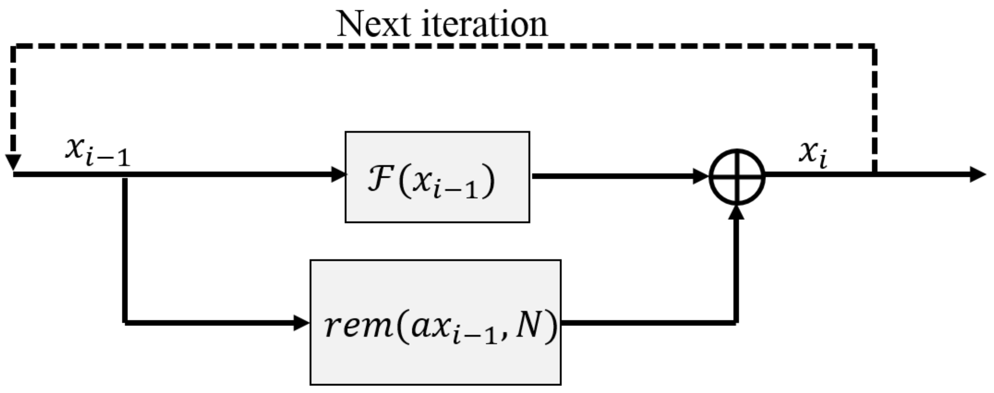
where a is a scaling factor, and N can be chosen to map the remainder result on the interval $(-N,N)$. Thus, in each iteration, the map’s value is scaled by a factor a, and then its remainder by division with N is fed back into $\mathcal{F}\left(x_{i-1}\right)$ by addition, to generate the next value of the map. The process is graphically depicted in Figure 1. The addition of the remainder term is motivated by the use of the Renyi map [36,37]

$$x_i=\mathrm{mod}(a{x}_{i-1},1),$$

(5)

which showcases constant chaos for $a>1$. The Renyi map uses the modulo operator, which limits the result to a positive value. Here, though, this will be generalized by using the remainder operation, which will help in the resulting maps having a uniform distribution on the interval $(-N,N)$.

In the following, it is proven that the technique (4) increases the complexity of the original map (3).

Theorem 1.

The proposed map (4) achieves a higher LE compared to its source map (3), if a is chosen as

$$a>2\underset{x\in \mathbb{D}}{sup}\left|\dot{\mathcal{F}}\left(x\right)\right|,$$

(6)

where $\mathbb{D}$ is the domain of the map (4).

Proof. 

Let ${\lambda }_s$ be the LE of the source map (3). Assuming that $\mathcal{F}$ is almost everywhere differentiable on $(-N,N)$, the LE is given by

$${\lambda }_s=\underset{n\to \infty }{lim}\frac{1}{n}\sum _{i=0}^{n-1}ln\left|\dot{\mathcal{F}}\left(x_i\right)\right|.$$

(7)

Now, assuming that $a{x}_{i-1}\in (-N,N)$, the LE for the proposed map (4) is

$$\begin{array}{ccc}\hfill {\lambda }_{mod}& =& \underset{n\to \infty }{lim}\frac{1}{n}\sum _{i=0}^{n-1}ln|\dot{\mathcal{F}}\left(x_i\right)+a|\hfill \\ & =& \underset{n\to \infty }{lim}\frac{1}{n}\sum _{i=0}^{n-1}ln\left|\dot{\mathcal{F}}\left(x_i\right)\left(1+\frac{a}{\dot{\mathcal{F}}\left(x_i\right)}\right)\right|\hfill \\ & =& \underset{n\to \infty }{lim}\frac{1}{n}\sum _{i=0}^{n-1}ln\left(\left|\dot{\mathcal{F}}\left(x_i\right)\right|\left|1+\frac{a}{\dot{\mathcal{F}}\left(x_i\right)}\right|\right)\hfill \\ & =& \underset{n\to \infty }{lim}\frac{1}{n}\sum _{i=0}^{n-1}ln\left|\dot{\mathcal{F}}\left(x_i\right)\right|+\underset{n\to \infty }{lim}\frac{1}{n}\sum _{i=0}^{n-1}ln\left|1+\frac{a}{\dot{\mathcal{F}}\left(x_i\right)}\right|\hfill \\ & =& {\lambda }_s+\underset{n\to \infty }{lim}\frac{1}{n}\sum _{i=0}^{n-1}ln\left|1+\frac{a}{\dot{\mathcal{F}}\left(x_i\right)}\right|,\hfill \end{array}$$

(8)

where we assume, as usual, $\dot{\mathcal{F}}\left(x_i\right)\ne 0$ for all points in a chaotic trajectory. From the above, when $\left|1+\frac{a}{\dot{\mathcal{F}}\left(x_i\right)}\right|>1$, $\forall x_i$, it will hold that ${\lambda }_{mod}>{\lambda }_s$. For $a>0$, this can be achieved regardless of the sign of $\dot{\mathcal{F}}\left(x_i\right)$ if we choose a as in (6).

A suitable choice would be

$$a=(e^k+1)\underset{x\in \mathbb{D}}{sup}\left|\dot{\mathcal{F}}\left(x\right)\right|,k>0,$$

(9)

for which we obtain

$$\begin{array}{ccc}\hfill \left|1+\frac{a}{\dot{\mathcal{F}}\left(x_i\right)}\right|& =& \left|1+\frac{(e^k+1)sup{|}_{x\in \mathbb{D}}\dot{\mathcal{F}}\left(x\right)|}{\dot{\mathcal{F}}\left(x_i\right)}\right|\hfill \\ & \ge & \left|\left|\frac{(e^k+1){sup}_{x\in \mathbb{D}}\left|\dot{\mathcal{F}}\left(x\right)\right|}{\dot{\mathcal{F}}\left(x_i\right)}\right|-\left|1\right|\right|\hfill \\ & \ge & (e^k+1)-1\hfill \\ & =& e^k.\hfill \end{array}$$

(10)

Thus, for the LE ${\lambda }_{mod}$, it holds that

$$\begin{array}{ccc}\hfill {\lambda }_{mod}& =& {\lambda }_s+\underset{n\to \infty }{lim}\frac{1}{n}\sum _{i=0}^{n-1}ln\left|1+\frac{a}{\dot{\mathcal{F}}\left(x_i\right)}\right|\hfill \\ \hfill & \ge & {\lambda }_s+\underset{n\to \infty }{lim}\frac{1}{n}\sum _{i=0}^{n-1}ln{e}^k\hfill \\ & =& {\lambda }_s+\underset{n\to \infty }{lim}\frac{1}{n}\sum _{i=0}^{n-1}k\hfill \\ \hfill & =& {\lambda }_s+\underset{n\to \infty }{lim}\frac{nk}{n}\hfill \\ \hfill & =& {\lambda }_s+k.\hfill \end{array}$$

(11)

Hence, the exponent can be increased arbitrarily. For an increase of k units, the control parameter a needs to increase exponentially with respect to k. □

Remark 1.

Note that the assumption $\dot{\mathcal{F}}\left(x_i\right)\ne 0$ does not lead to loss of generality. In the special case where there exists a point $x_i$ in the map’s orbit for which $\dot{\mathcal{F}}\left(x_i\right)=0$, the original map (3) would exhibit a superstable orbit with an LE that goes to minus infinity. Superstable periodic orbits are those for which the product of the map’s derivative along the orbit (whose logarithm of the absolute value produces the LE) is zero. It is sufficient that a periodic orbit has one point with zero derivative for it to be a superstable orbit. In this case, though, the LE of the updated map (4) is

$${\lambda }_{mod}=\underset{n\to \infty }{lim}\frac{1}{n}\sum _{i=0}^{n-1}ln\left|a\right|,$$

(12)

which can be treated in the same way considering (9). Hence, the superstable orbits of the original map are vanished. Moreover, the proposed map (4) would exhibit superstable orbits for any point $x_i$ such that

$$\dot{\mathcal{H}}\left(x_i\right)=0\Rightarrow \dot{\mathcal{F}}\left(x_i\right)+a=0$$

(13)

However, for a chosen as (6), the above condition will not hold for any $x_i$. Hence, the superstable orbits of the proposed map will also vanish.

Overall, Theorem 1 provides a sufficient condition for the loss of stability of the periodic orbits. This means that not only the LE is increased, but we also give conditions for which all the superstable periodic orbits are destroyed, and conditions for which periodic orbits are no longer stable. Periodic windows appear in the neighborhood of superstable orbits [38]. Thus, their elimination contributes to making the chaos more robust.

In the following, a result on the stability of the map’s equilibria is provided.

Theorem 2.

The equilibria of the map (4) are unstable, for parameter a chosen as in (9), for a positive $k>0$ that satisfies

$$k>ln\frac{1}{|\dot{\mathcal{F}}\left(x^{\ast }\right)|}$$

(14)

Proof. 

The equilibria $x^{\ast }$ of (4) are given by

$$x^{\ast }=\mathcal{F}\left(x^{\ast }\right)+\mathrm{rem}(a{x}^{\ast },N).$$

(15)

Now, considering the derivative of the map’s function $\mathcal{H}\left(x\right)$, assuming again that $\mathcal{F}$ is almost everywhere differentiable on $(-N,N)$, and $a{x}_{i-1}\in (-N,N)$,

$$\dot{\mathcal{H}}\left(x\right)=\dot{\mathcal{F}}\left(x\right)+a.$$

(16)

For the equilibria (15) to be stable, it should hold that $|\dot{\mathcal{H}}\left(x^{\ast }\right)|<1$. Let a be chosen as in (9). This yields

$$\begin{array}{ccc}\hfill |\dot{\mathcal{H}}\left(x^{\ast }\right)|& =& \left|\dot{\mathcal{F}}\left(x^{\ast }\right)+(e^k+1)\underset{x\in \mathbb{D}}{sup}\left|\dot{\mathcal{F}}\left(x\right)\right|\right|\hfill \\ & \ge & \left|\left|(e^k+1)\underset{x\in \mathbb{D}}{sup}\left|\dot{\mathcal{F}}\left(x\right)\right|\right|-\left|\dot{\mathcal{F}}\left(x^{\ast }\right)\right|\right|\hfill \\ & =& (e^k+1)\underset{x\in \mathbb{D}}{sup}|\dot{\mathcal{F}}\left(x\right)|-|\dot{\mathcal{F}}\left(x^{\ast }\right)|\hfill \\ & \ge & (e^k+1)|\dot{\mathcal{F}}\left(x^{\ast }\right)|-|\dot{\mathcal{F}}\left(x^{\ast }\right)|\hfill \\ & \ge & e^k\left|\dot{\mathcal{F}}\left(x^{\ast }\right)\right|,\hfill \end{array}$$

(17)

for $k>0$. By choosing a positive k that satisfies (14), we obtain

$$\begin{array}{ccc}\hfill |\dot{\mathcal{H}}\left(x^{\ast }\right)|& >& e^{ln\frac{1}{|\dot{\mathcal{F}}\left(x^{\ast }\right)|}}\left|\dot{\mathcal{F}}\left(x^{\ast }\right)\right|\hfill \\ & =& \frac{1}{|\dot{\mathcal{F}}\left(x^{\ast }\right)|}\left|\dot{\mathcal{F}}\left(x^{\ast }\right)\right|\hfill \\ & =& 1\hfill \end{array}$$

(18)

Thus, the equilibria (15) will be unstable. □

2.2. Geometric Interpretation

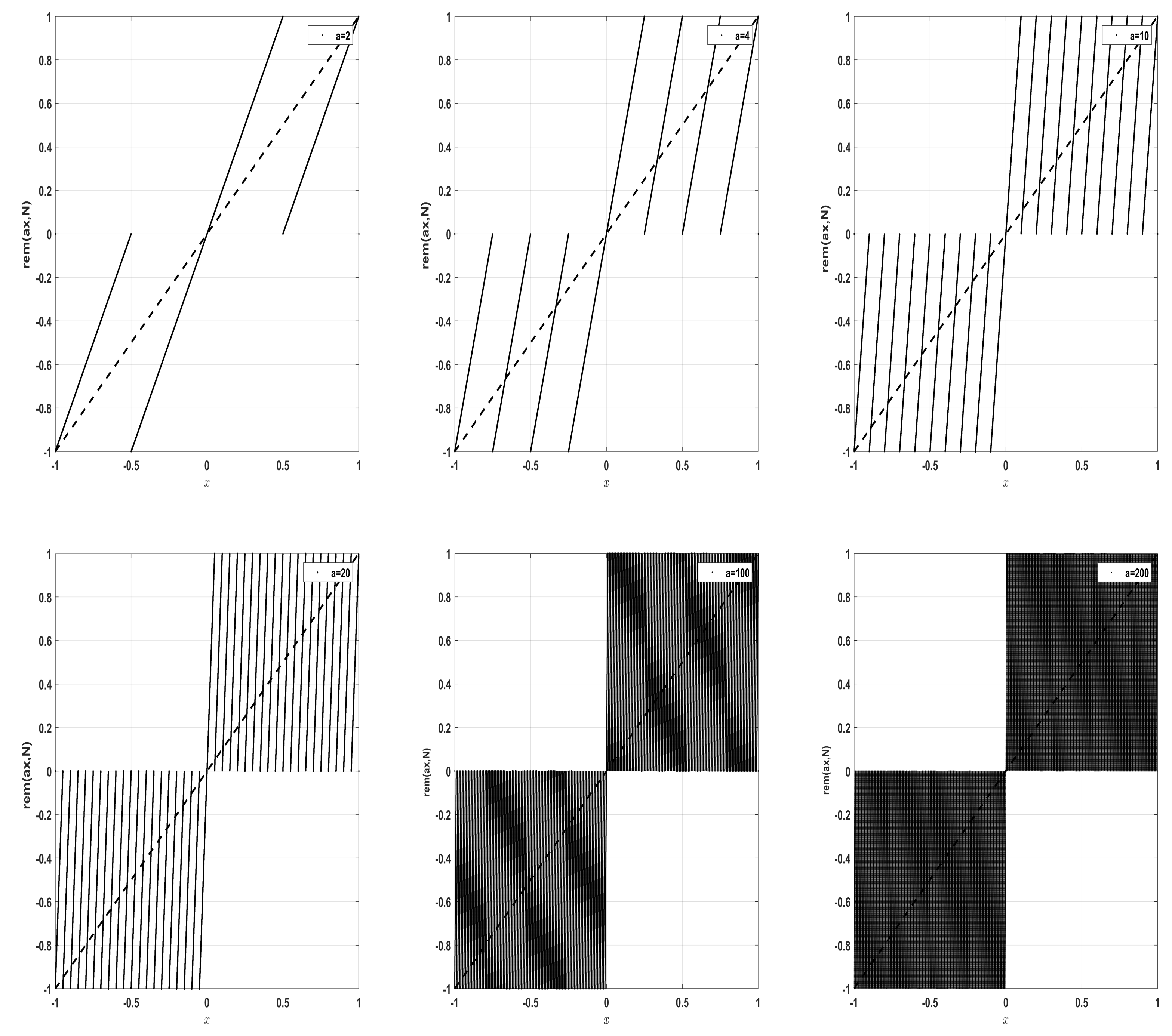
A second approach to study the effect of the addition of the remainder term $\mathrm{rem}(a{x}_{i-1},N)$ on a map is by considering its phase diagram. For discrete maps, the phase diagram depicts pairs of consecutive values $(x_{i-1},x_i)$. The relation between consecutive mappings can equivalently be depicted by plotting the function $\mathcal{F}\left(x\right)$ on the interval $x\in (-N,N)$. Figure 2 depicts the function $\mathrm{rem}(ax,N)$ for different values of the parameter a, and $N=1$. The function consists of discontinuous linear segments, due to the term $a{x}_{i-1}$ mapping outside the interval $(-1,1)$, which increases in number as the parameter a increases. Thus, when added in the map (4), this piecewise linear function will impose discontinuities in the source map’s function $\mathcal{F}\left(x\right)$. As the number of piecewise linear bands increases, the number of periodic orbits (all unstable assuming the condition set by Theorem 1) increases, as well as the derivative of the map, the latter leading to an increase in the LE. As topological entropy is defined by the logarithm of the number of unstable periodic orbits (UPOs) [39], one can see a direct increase in the entropy as well. The above lead to a system with higher complexity, as will be illustrated in Section 4.

2.3. Key Space

The key values of a map, as mentioned earlier in Section 1.2, refer to the set of parameters that are required to reproduce a chaotic trajectory. Based on the key values, the key space $\mathcal{K}$ is the number of all the possible parameter combinations that can be chosen to compute the map’s trajectory. The addition of the term $\mathrm{rem}(a{x}_{i-1},N)$ introduces two new parameters in the new map, $a,N$. Hence, the key space of the map is increased. Assuming an accuracy of 16 digits, this amounts to a multiplicative increase of size ${10}^{2·16}={10}^{32}\approx {\left({10}^3\right)}^{10.6}\approx {\left(2^{10}\right)}^{10.6}=2^{106}$. Thus, for an initial seed map with key space $\mathcal{K}$, the modified map will have a key space of $\mathcal{K}·2^{106}$. In

Table 1. Comparison of key space increase for different chaotification techniques.

Reference	Seed Map(s)	Modified Map
Present work	$\mathcal{K}$	$2^{106}·\mathcal{K}$
[17]	$\mathcal{K}$	$2^{53}·\mathcal{K}$
[18]	$\mathcal{K}$	$\mathcal{K}$
[19]	${\mathcal{K}}_i$	${\prod }_{i=1}^m{\mathcal{K}}_i$
[20]	${\mathcal{K}}_i$	$2^{53}{\prod }_{i=1}^m{\mathcal{K}}_i$
[21]	$\mathcal{K}$	$2^{53}·\mathcal{K}$
[22]	$\mathcal{K}$	$2^{106}·\mathcal{K}$
[24]	$\mathcal{K}$	$2^{53}·\mathcal{K}$
[23]	$\mathcal{K}$	$2^{53}·\mathcal{K}$
[32]	${\mathcal{K}}_i$	$2^{53m}{\prod }_{i=1}^m{\mathcal{K}}_i$

, a comparison of the key space increases for different techniques is provided. The proposed technique is among the most efficient with respect to key space increase. Note that the key space calculations in this table correspond to all possible parameter pairs, some of which may yield non-chaotic behavior. However, in the proposed scheme, chaotic behavior can always be guaranteed.

2.4. Limitations

One drawback that can be identified for the proposed technique inspired by (2) is that it cannot be applied to polynomial maps on an interval to improve their behavior. For example, this technique will fail to improve the behavior of the classic logistic map, as the new map (4) will have a trajectory that goes to infinity. This drawback, however, can be circumvented by adding to (4) an amplitude parameter that decreases the values coming out of the remainder operation, and by choosing a polynomial map parameter that sets the trajectory within an interval smaller than that permitted to the domain of the chaotic map. For example, choosing $\mathcal{F}$ to be as in (1), one can set $k<4$, and the reminder term would be rewritten as $C\mathrm{rem}(a{x}_{i-1},N)$, with $C<1$. This is, however, beyond the scope of this work.

A common issue that emerges when considering digital implementations of chaos-based cryptography schemes is the reproducibility of chaotic maps on different devices [29,40,41]. As nonlinear systems are sensitive to operator accuracy, round-off errors in the least significant digits can quickly blow up over very few iterations, yielding different trajectories across different devices, despite having the same initial conditions and parameter values. Thus, in the application of encryption and secure communications where data are exchanged, to achieve output matching for the same chaotic map that is simulated on different devices, all devices should be adjusted to match the accuracy of the device with the lowest processing power.

Moreover, as the proposed technique is based on mixing the most significant bits of the map with its least significant, it is important to choose the parameter a according to the device capabilities, to avoid overflows. For example, in a microcontroller capable of performing floating point operations using a memory of 6 digits, choosing $a>{10}^7$ will result in overflowing. The above are issues that are under study and will be taken into account for future hardware implementations of the proposed technique.

3. Generalizations

The proposed methodology can be generalized by considering the addition of multiple remainder operators, each with a different parameter, as follows

$$x_i=\mathcal{H}\left(x_{i-1}\right)=\mathcal{F}\left(x_{i-1}\right)+\sum _{j=1}^m\mathrm{rem}(a_j{x}_{i-1},N),$$

(19)

where $a_j>0$ are the control parameters, and $m\in \mathbb{N}$. This would result in an even stronger mixing of the map’s digits in each iteration. This increase in the summation terms would, however, need to take into consideration the computational cost for its implementation in order not to impact the efficiency of the method.

Moreover, the proposed methodology can be extended by considering the addition with the remainder of any nonlinear function $\mathcal{G}$, i.e.,

$$x_i=\mathcal{F}\left(x_{i-1}\right)+\mathrm{rem}(\mathcal{G}\left(x_{i-1}\right),N).$$

(20)

Here, polynomials, sinusoidal functions, or their combination can be used to improve performance. In this work, the choice was made for the simplest linear term, so as to improve complexity but keep the computational load to the minimum. Since the linear term yielded positive results, it can be assumed with relative certainty that other nonlinear functions will also work. This will be explored in future works.

A case of particular interest is that of setting $\mathcal{G}=a\mathcal{F}$. The results for this case are described in the following theorem.

Theorem 3.

The generalized map (20) with $\mathcal{G}=a\mathcal{F}$ achieves a higher LE compared to its source map (3), for $a>0$.

Proof. 

Following a similar procedure to the proof of Theorem 1 yields

$$\begin{array}{ccc}\hfill {\lambda }_{mod}& =& \underset{n\to \infty }{lim}\frac{1}{n}\sum _{i=0}^{n-1}ln|\dot{\mathcal{F}}\left(x_i\right)+\dot{\mathcal{G}}\left(x_i\right)|\hfill \\ & =& {\lambda }_s+\underset{n\to \infty }{lim}\frac{1}{n}\sum _{i=0}^{n-1}ln\left|1+\frac{\dot{\mathcal{G}}\left(x_i\right)}{\dot{\mathcal{F}}\left(x_i\right)}\right|\hfill \\ & =& {\lambda }_s+\underset{n\to \infty }{lim}\frac{1}{n}\sum _{i=0}^{n-1}ln\left|1+a\right|.\hfill \end{array}$$

(21)

Thus, we obtain ${\lambda }_{mod}>{\lambda }_s$ for $a=(e^k+1)$, $k>0$. □

4. Simulations for Different Source Maps

In this section, the proposed chaotification technique will be tested on different one-dimensional maps.

4.1. Simplest Linear Map

Initially, a simple linear map is considered, of the form

$$x_i=\frac{1}{k}{x}_{i-1}.$$

(22)

The above map is linear, and hence cannot exhibit chaotic behavior. The map has a unique solution, the equilibrium point at 0, which is stable if its eigenvalue lies within the unit circle, which holds if $\left|k\right|>1$. The above map is modified based on the proposed technique, yielding

$$x_i=\frac{1}{k}{x}_{i-1}+\mathrm{rem}(a{x}_{i-1},N).$$

(23)

Based on Theorem 1, since $\frac{d}{dx}\left(\frac{1}{k}x\right)=\frac{1}{k}$, we can set $a>2$ to destroy the stability of the equilibrium point and increase the map’s LE.

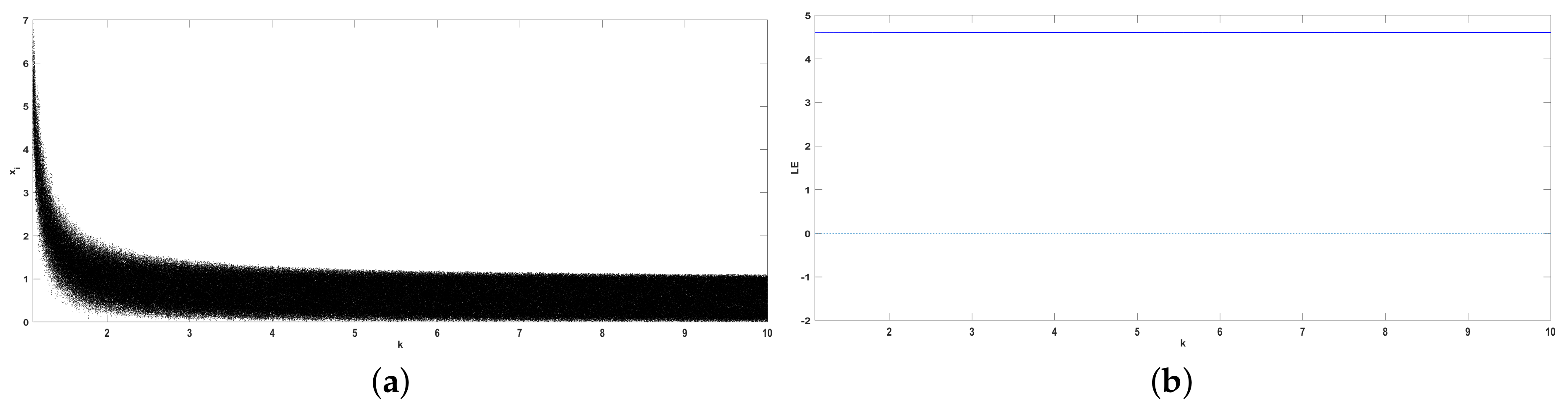
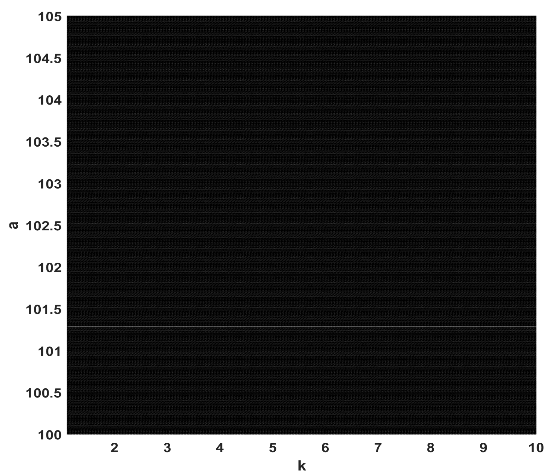
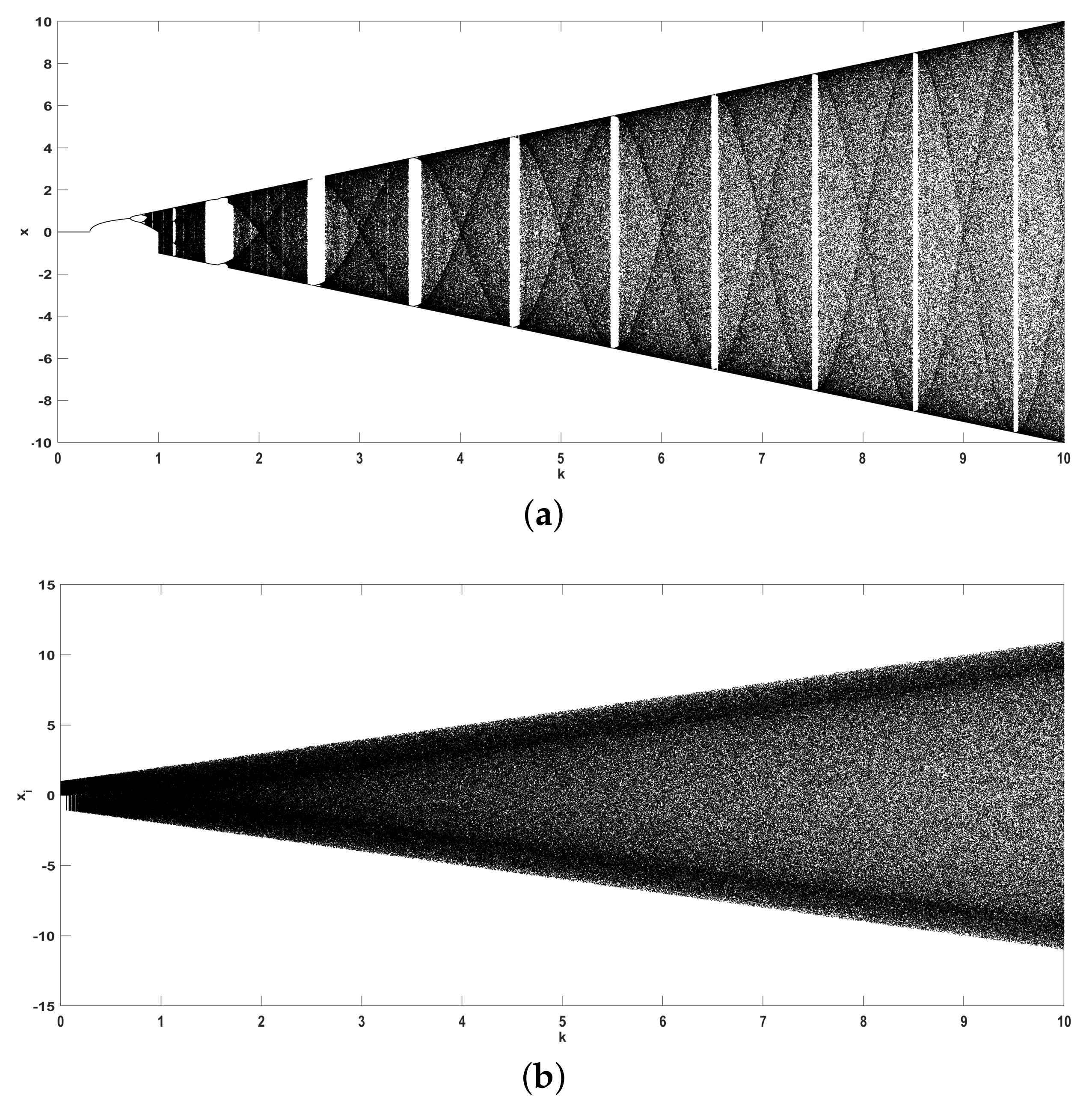
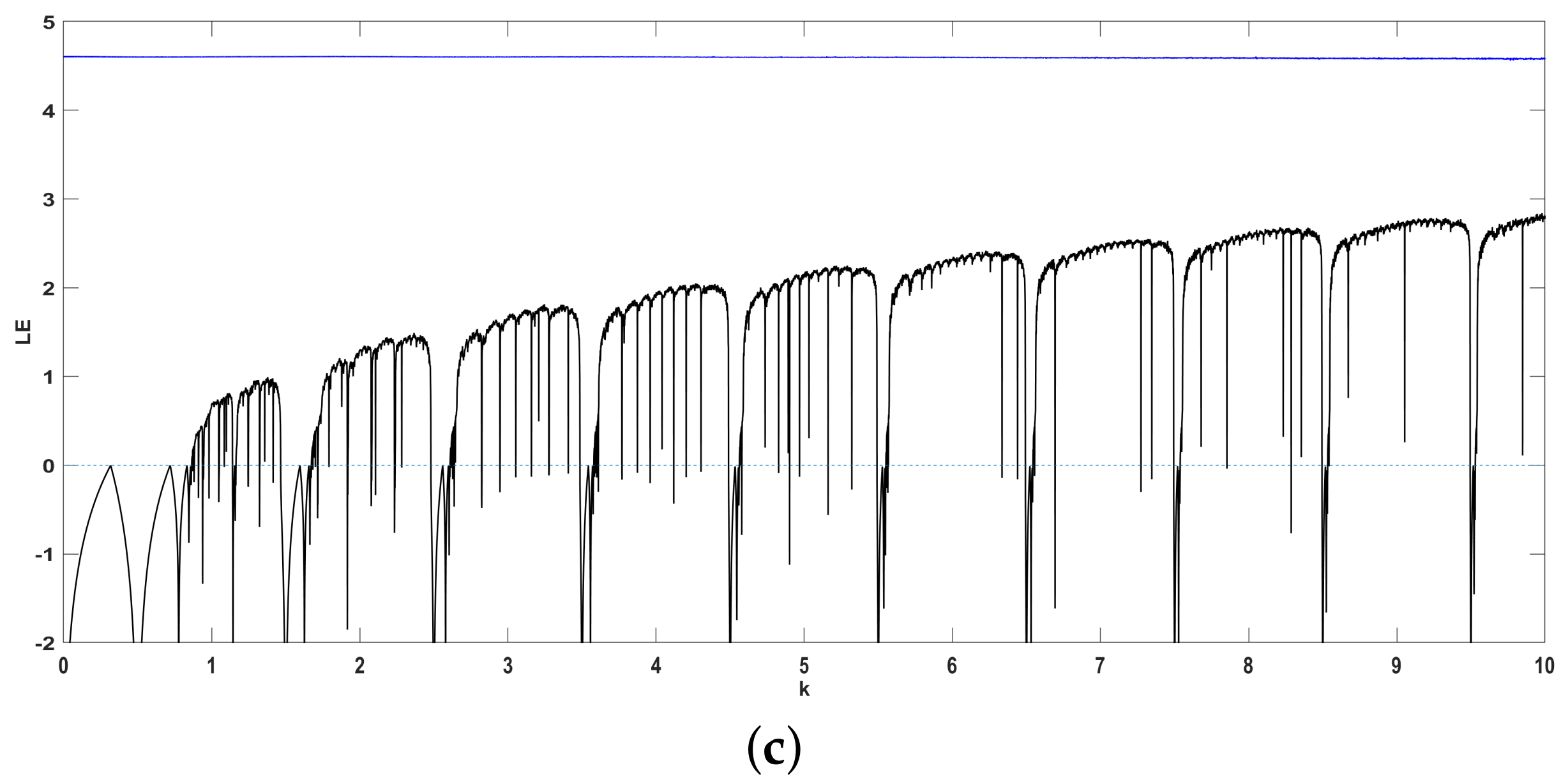
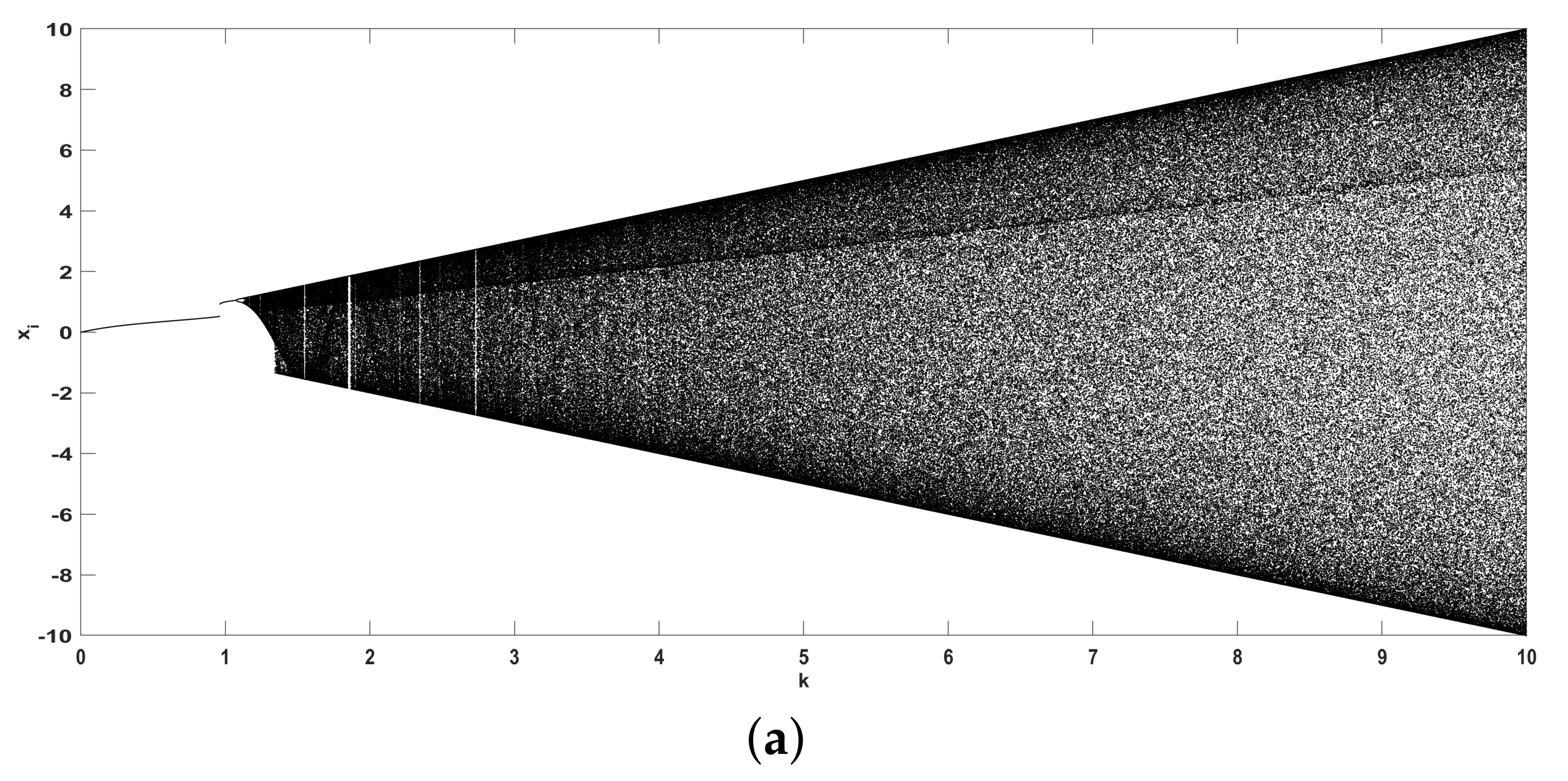
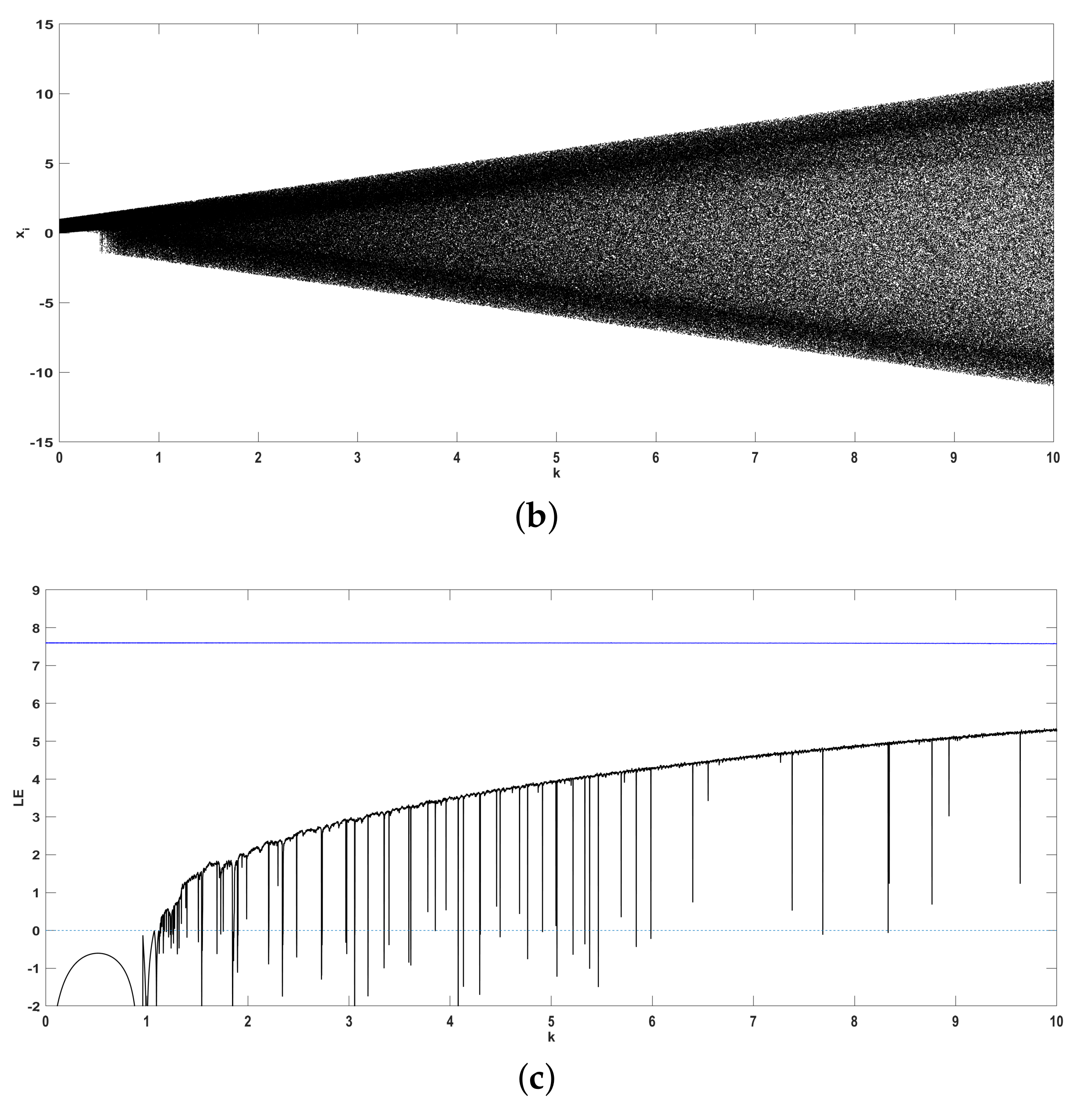
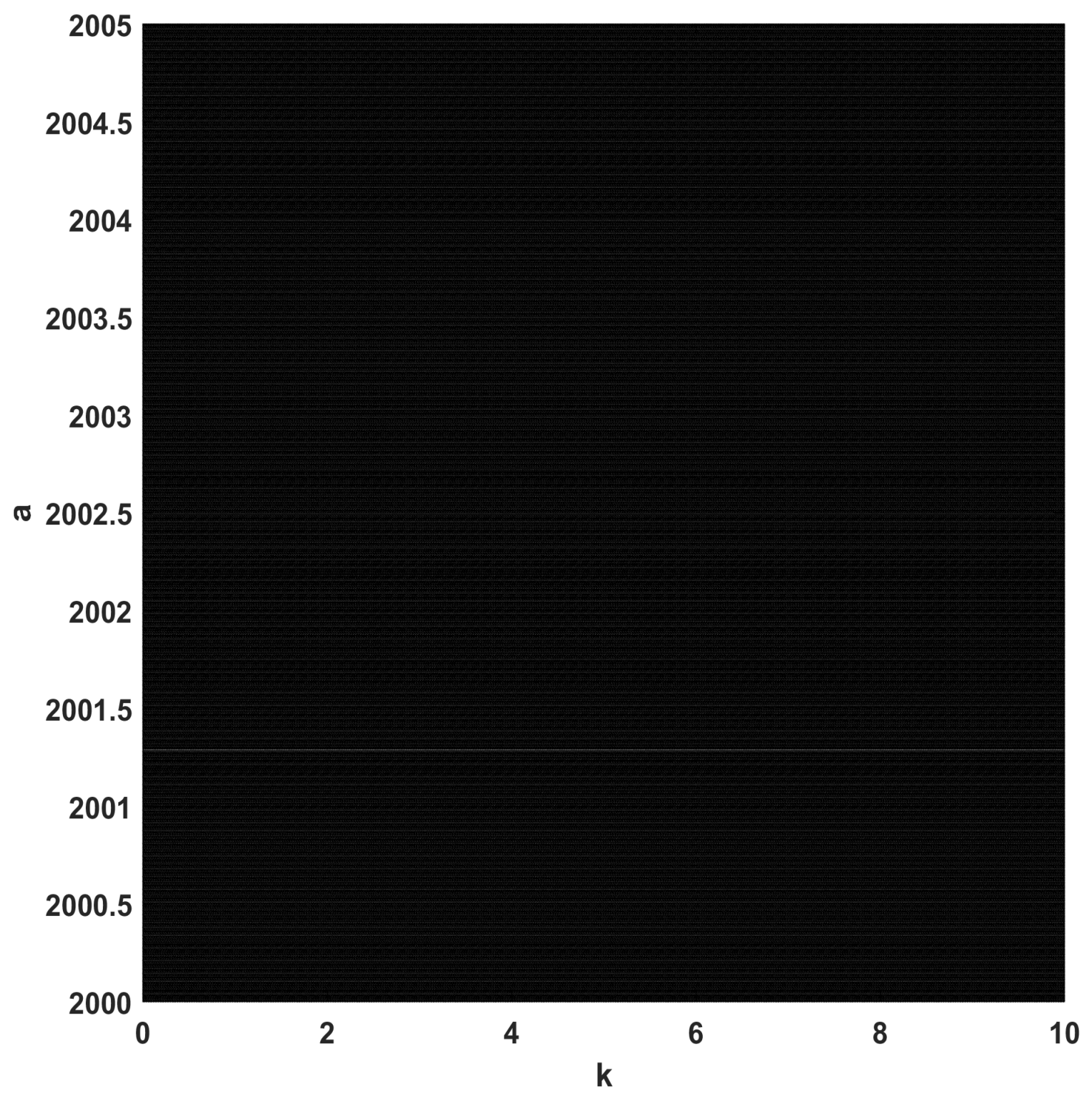
Figure 3a shows the bifurcation diagram of (23) with respect to k, for $a=100$ and $N=1$. It can be seen that the modified map is indeed chaotic. This can be verified from its LE, shown in Figure 3b. In Figure 4, the parameter pairs $(k,a)$ that correspond to chaotic behavior are shown. The parameters are chosen to satisfy the condition in Theorem 1, and, as such, the parameter space is compact, without holes, guaranteeing robust chaos.

Moreover, Figure 5 shows the cobweb plot of the original (22) and modified map (23) for $k=10$, with a very distinct oscillatory pattern.

4.2. Sine Map

Consider the well-known sine map [42,43,44]

$$x_i=ksin\left(\pi x_{i-1}\right),$$

(24)

and the new map based on the proposed technique is

$$x_i=ksin\left(\pi x_{i-1}\right)+\mathrm{rem}(a{x}_{i-1},N).$$

(25)

In the following, we fix $N=1$. Based on the proof of Theorem 1, since $\frac{d}{dx}(ksin\left(\pi x\right))=k\pi cos\left(\pi x\right)$, we can set $a>2k\pi$ to destroy the stability of the periodic orbits, increase the number of UPOs, and increase the map’s LE. Here, we choose $a=100$.

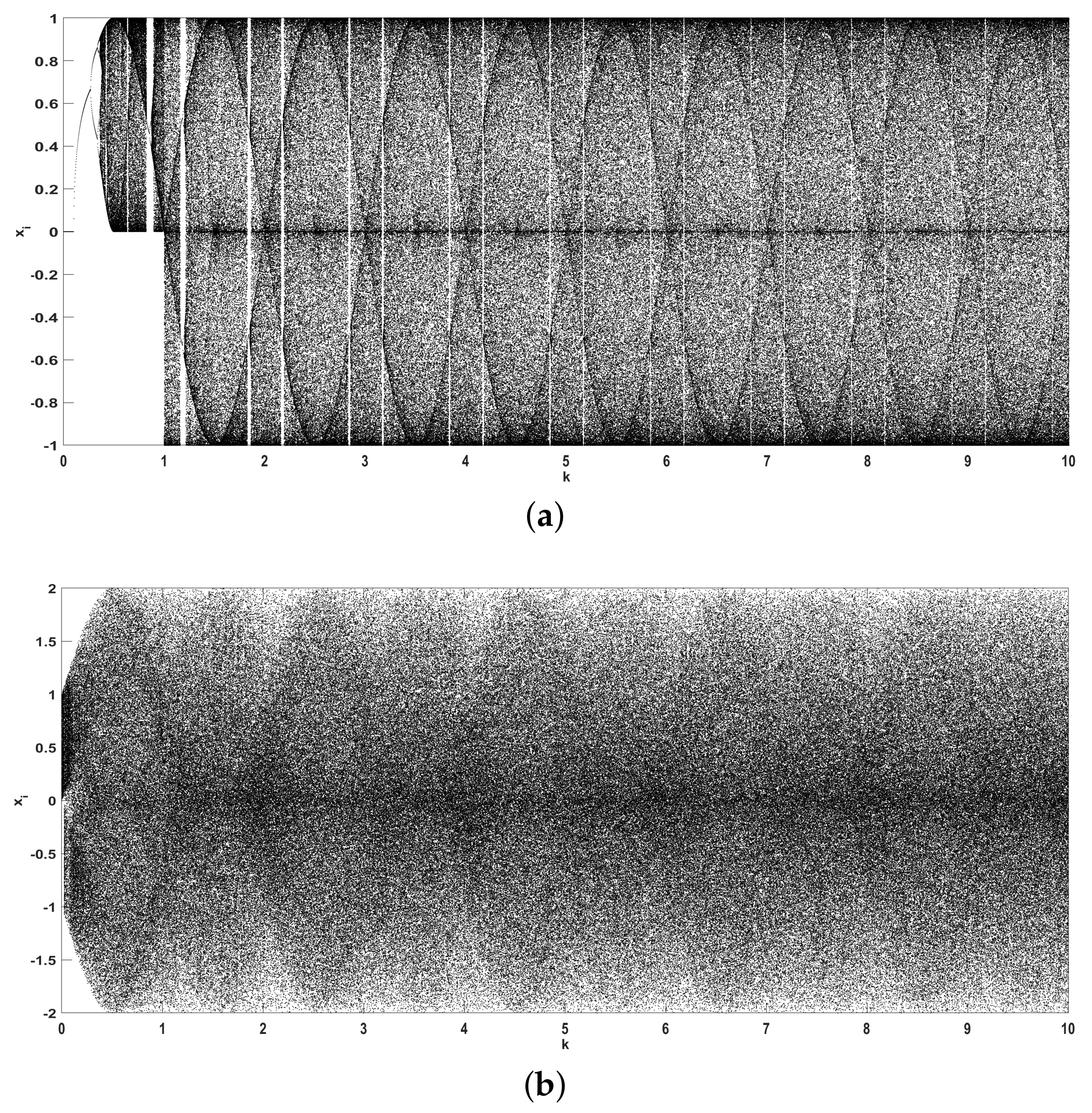
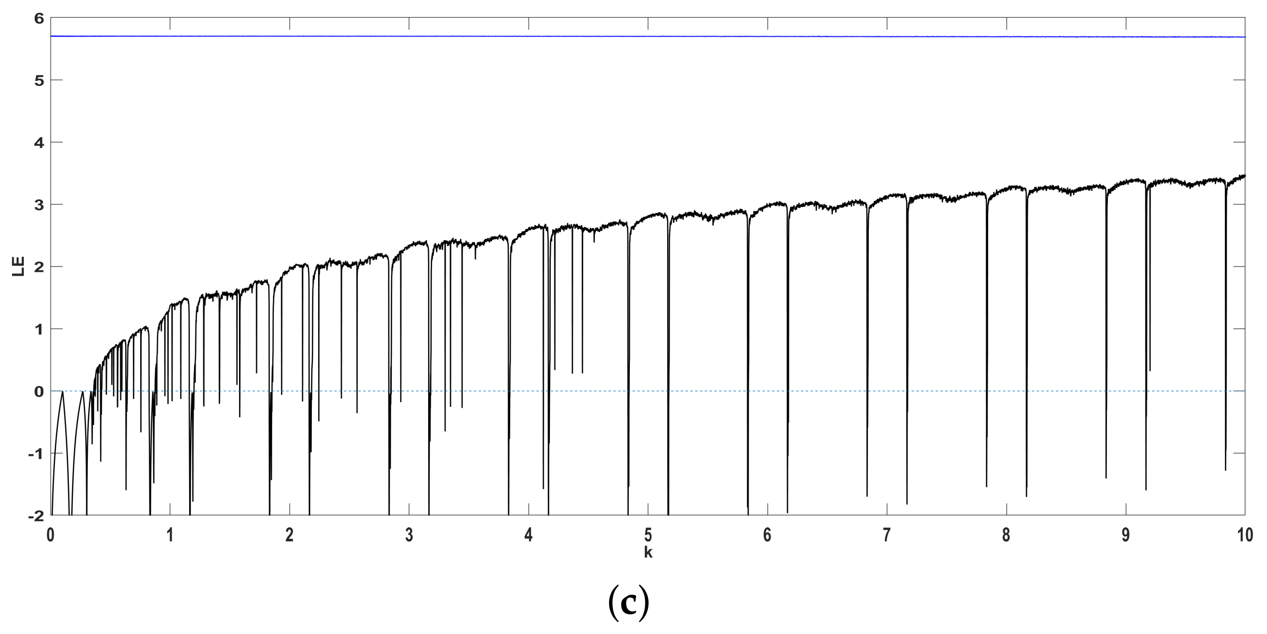
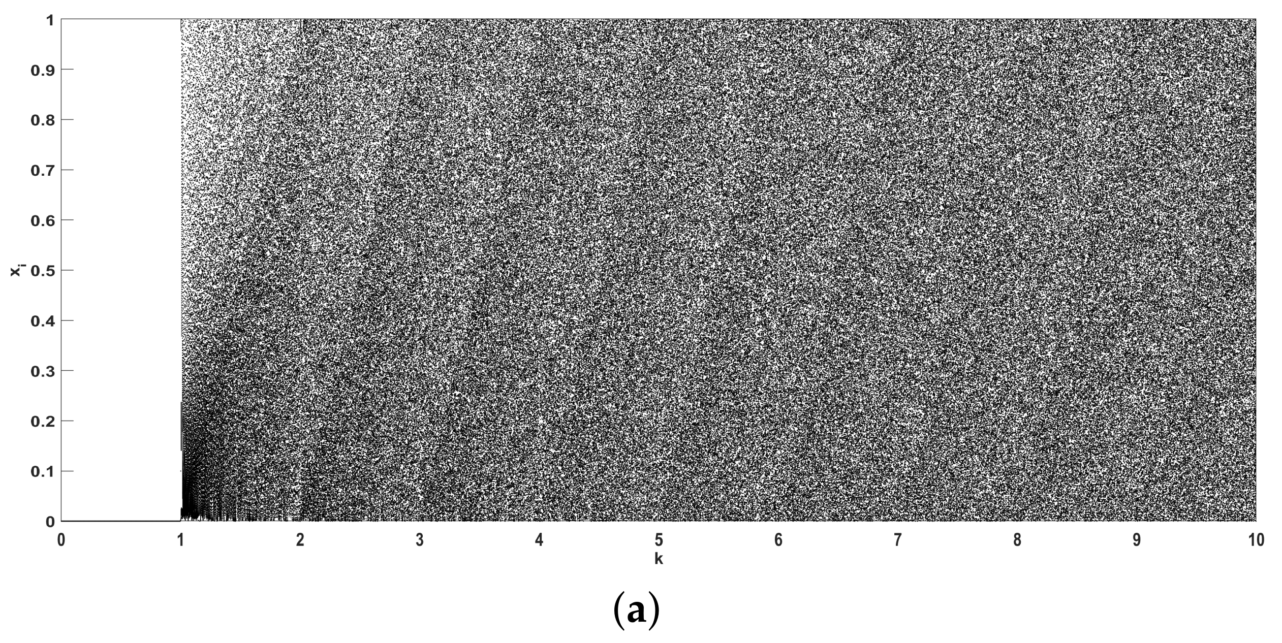
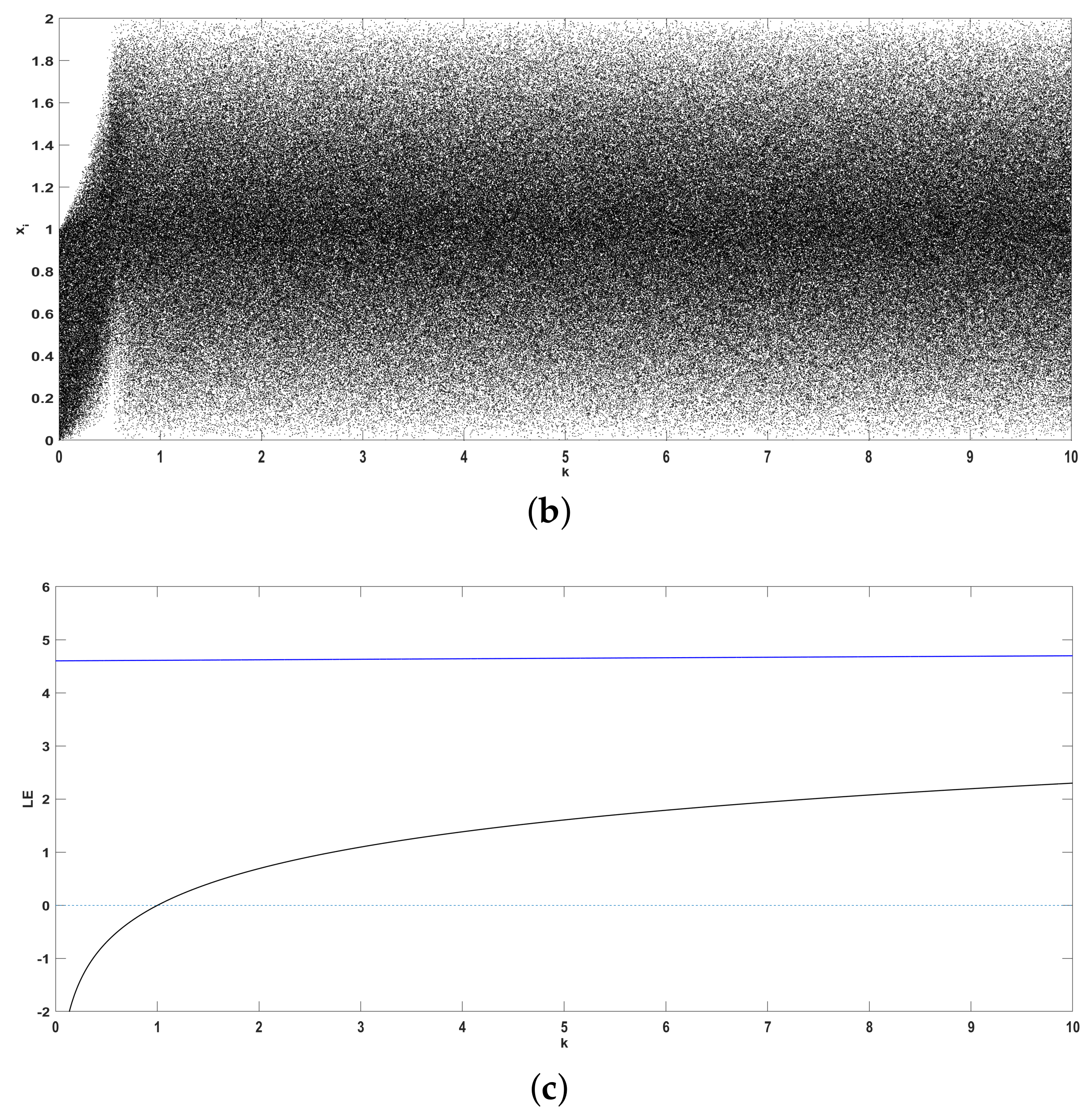
Figure 6a,b depict the bifurcation diagrams of the original sine map (24) and modified sine map (25) with respect to parameter k, for $a=100$. It can be seen that while the sine map exhibits periodic windows, the modified map has uninterrupted chaotic behavior for a dense and compact set of the given parameter range. This can be verified by the LE diagram in Figure 6c. Whereas the LE of the original map (black) has negative values and drops, indicating the location of the superstable periodic orbits, the LE of the modified map is constant for a dense and compact range of the paremeter b.

Moreover, Figure 7 depicts a diagram that showcases the periodic and chaotic regions of the modified map (25), for different parameter pairs $(k,a)$ and $N=1$. All the parameter pairs $(k,a)$ result in chaotic behavior.

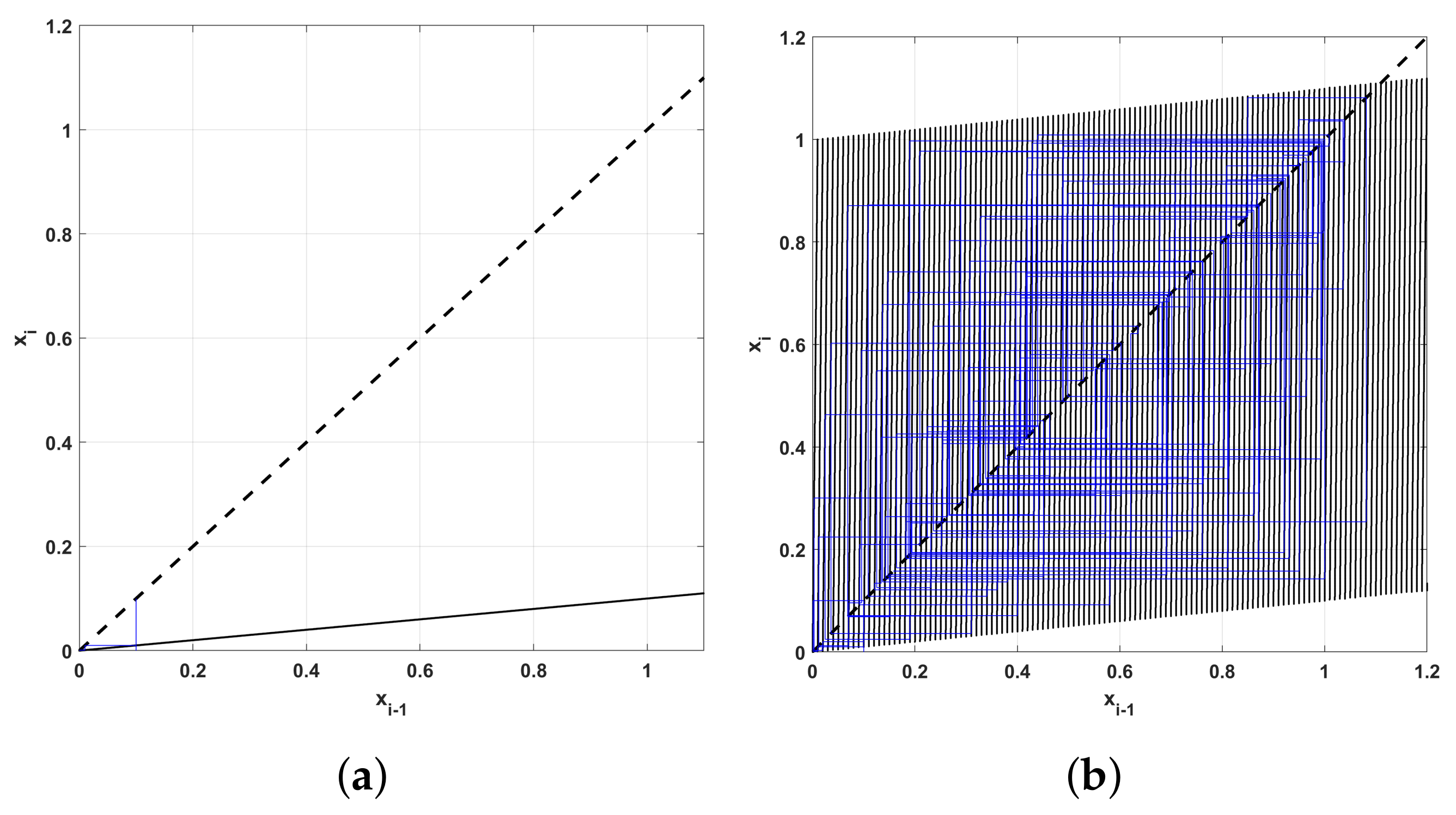
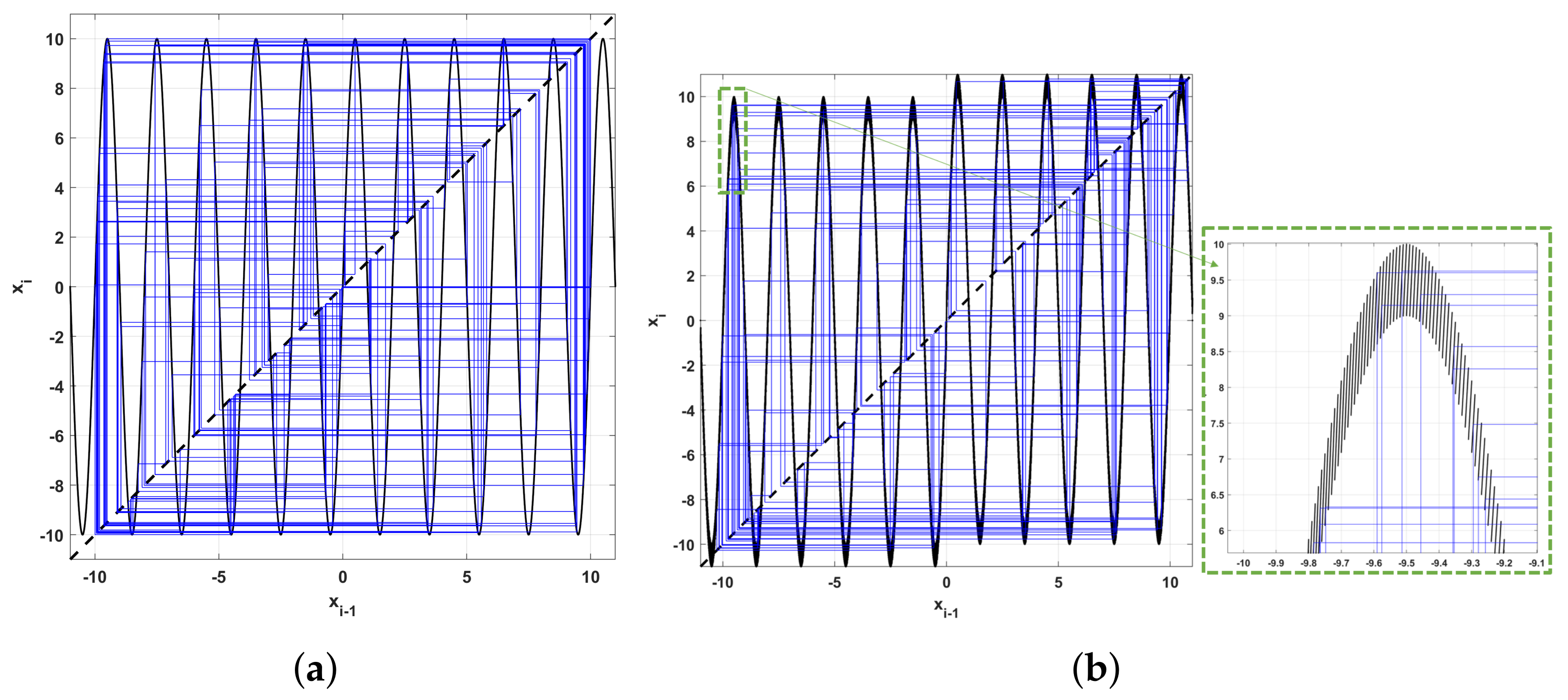
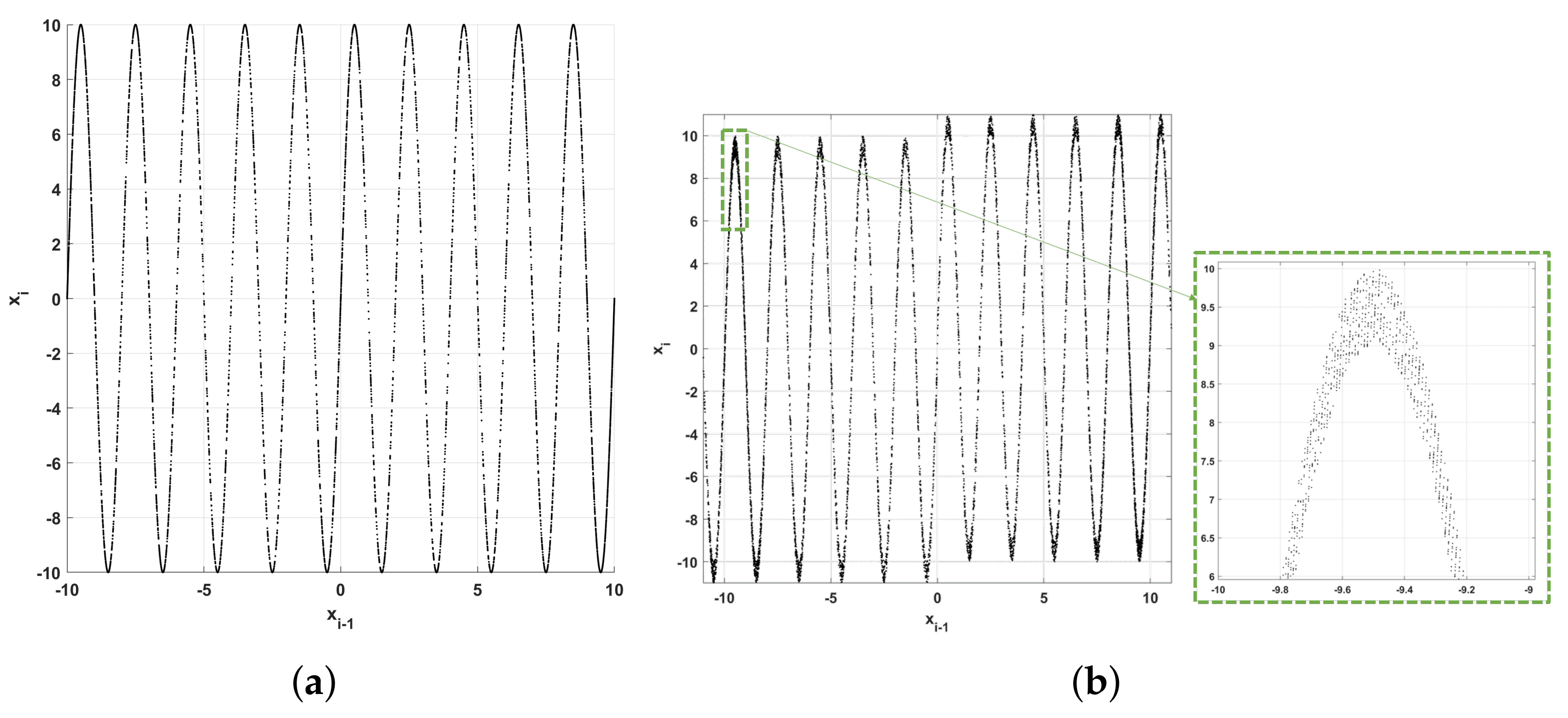
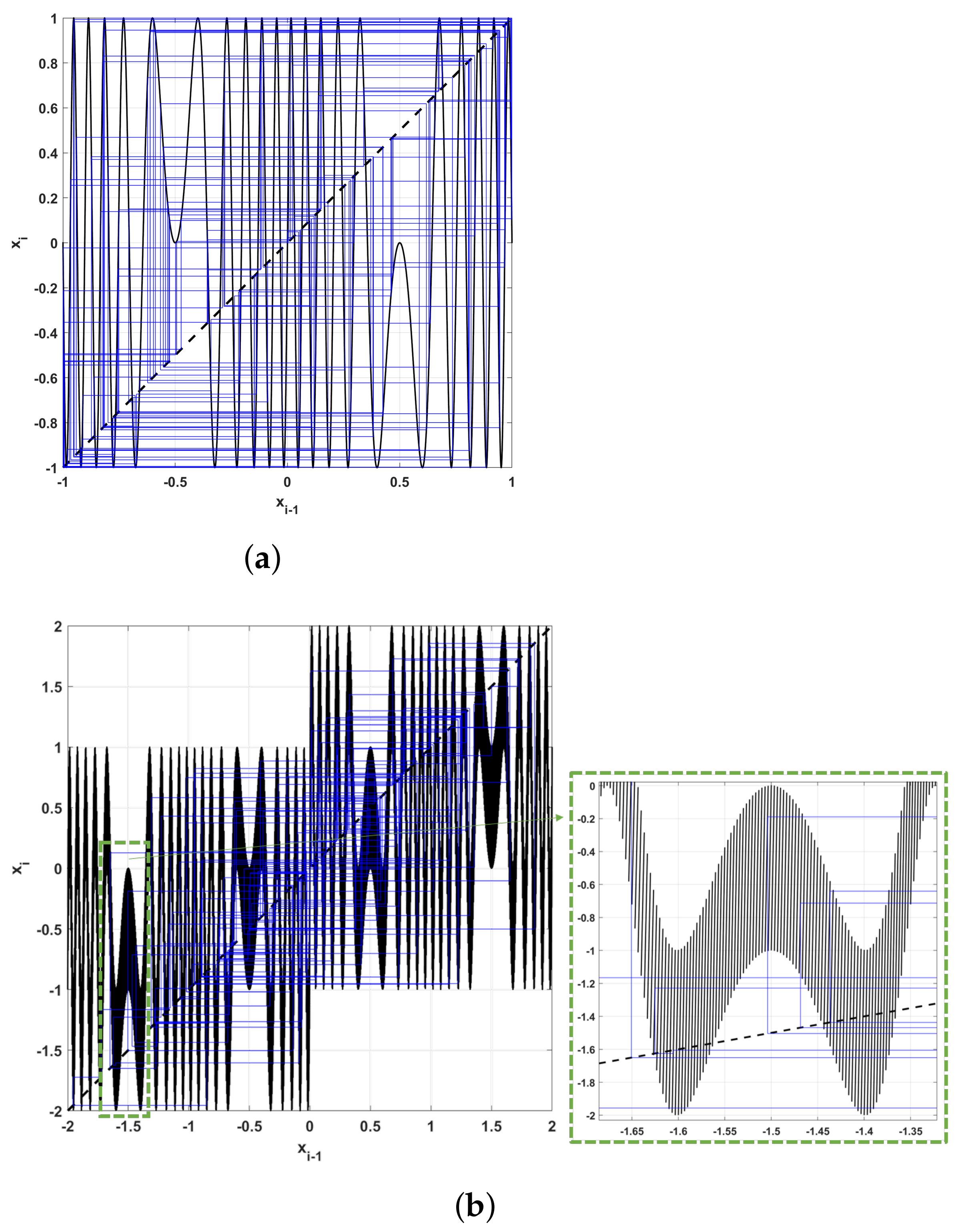
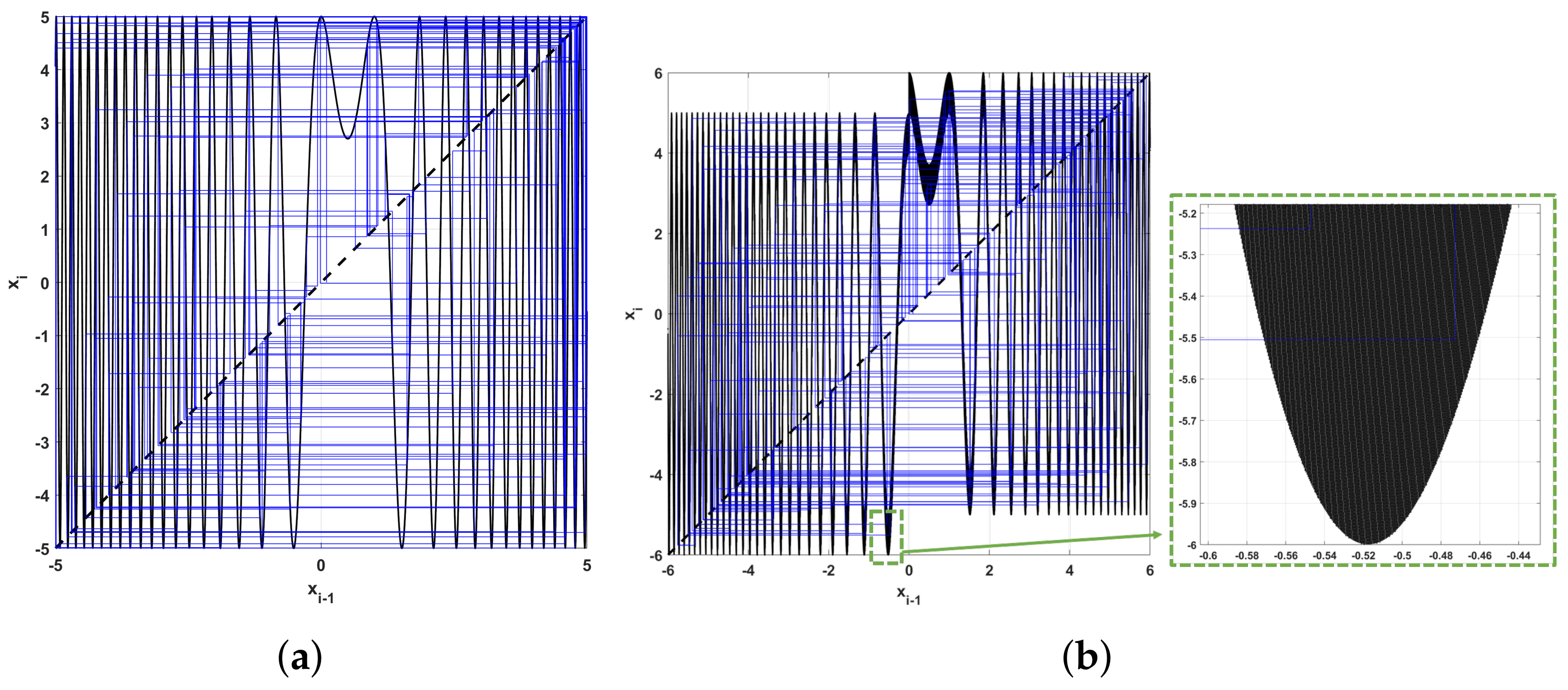
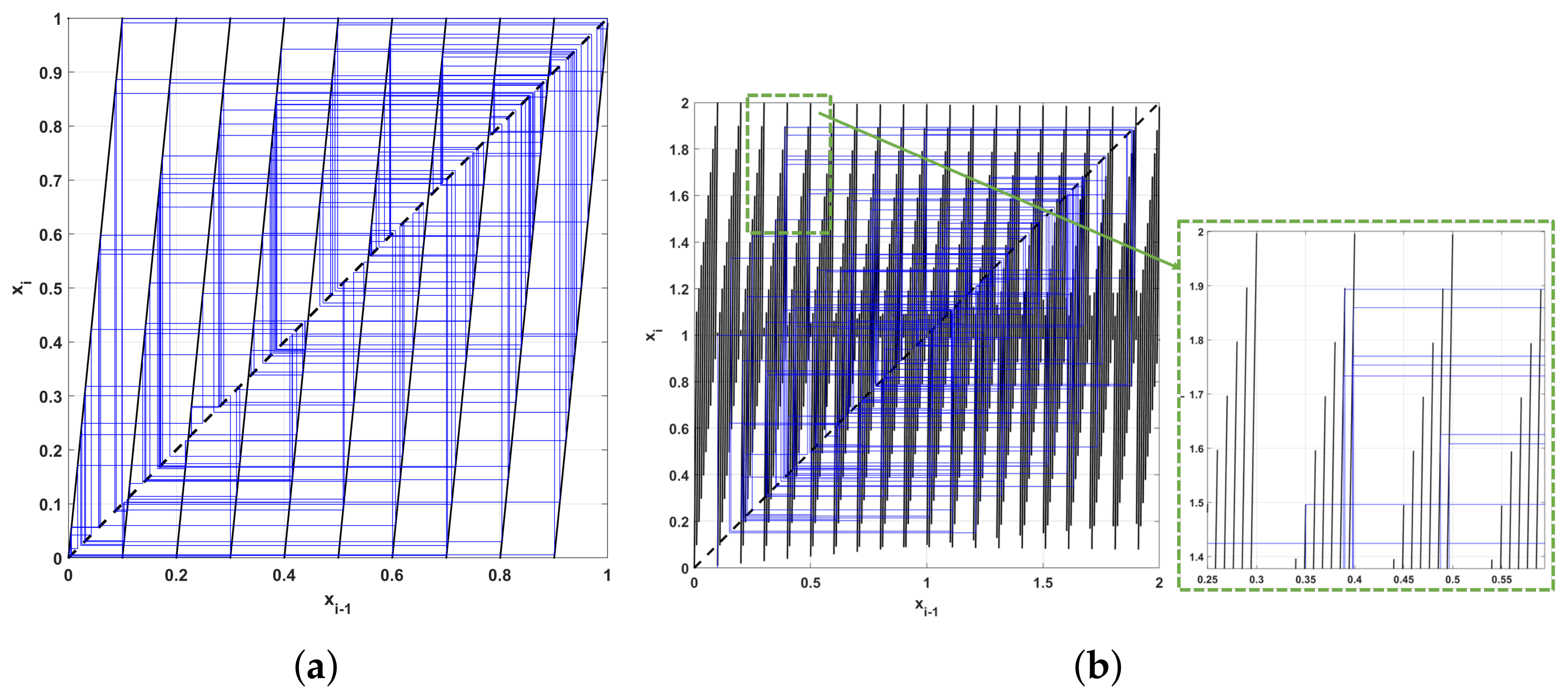
Finally, Figure 8 depicts two cobweb diagrams for the original and modified maps. Here, the effect of the remainder term can be observed clearly in the close-up subregion. While the map attains a diagram similar to the original map, the curve now is discontinuous. Two phase diagrams are also separately depicted in Figure 9 for clarity. Interestingly, both in the cobweb and phase diagrams, the modified map appears to inherit a seemingly stochastic characteristic, where the mapping of a point seems to be mapped at different places. There is no stochasticity, of course, as this phenomenon is due to the multiple piecewise lines very close to each other. This also appears for the rest of the maps that are considered.

4.3. Sine–Sine Map

In [18], a chaotification technique was proposed through the composition of any chaotic map with a sine function. The authors proposed various enhanced versions of existing maps to showcase their results. One of the proposed maps was the sine–sine map described by

$$x_i=sin(\pi ksin\left(\pi x_{i-1}\right)).$$

(26)

Here, the above map is modified as

$$x_i=sin(\pi ksin\left(\pi x_{i-1}\right))+\mathrm{rem}(a{x}_{i-1},N).$$

(27)

Based on Theorem 1, since $\frac{d}{dx}(sin(\pi ksin\left(\pi x\right)))=k{\pi }^{2}cos\left(\pi x\right)cos(k\pi sin\left(\pi x\right))$, we can set $a>2k{\pi }^2$. Thus, for the range $k\in [0,10]$, we require $a>197.3921$, in order for all the periodic orbits to be unstable, and the LE to become positive. Here, we set $a=300$.

Bifurcation diagrams are shown in Figure 10a,b. Observe that the map (27) proposed in [18] has periodic regions, but the map (27) exhibits uninterrupted chaotic behavior for the range of considered parameters, as can be verified by the LE diagram in Figure 10c. The diagram in Figure 11 verifies that all parameter pairs in the chosen range yield chaotic behavior.

Moreover, Figure 12 shows two cobweb diagrams for the original (26) and modified map (27), where the effect of the discontinuities introduced by the remainder addition is graphically seen.

4.4. Cosine-Logistic Map

Similar to the sine chaotification technique in [18], a cosine chaotification was proposed in [20]. The authors presented several enhanced versions of classic maps. As an example, consider the cosine-logistic map

$$x_i=kcos\left(r{x}_{i-1}(1-x_{i-1})\right).$$

(28)

The proposed modified map is

$$x_i=kcos\left(r{x}_{i-1}(1-x_{i-1})\right)+\mathrm{rem}(a{x}_{i-1},N).$$

(29)

Since $\frac{d}{dx}\left(kcos\left(rx(1-x)\right)\right)=kr(2x-1)sin\left(rx(1-x)\right)$, the control parameter can be set as $a>2kr{sup}_{x\in \mathbb{D}}(2x-1)$. Here, we set $r=4$. Thus, for the range $k\in [0,10]$, we can choose $a>1600$, so we set $a=2000$.

The bifurcation diagrams for the two maps are shown in Figure 13a,b, along with the LE diagram in Figure 13c. Again, the periodic regions that were present in the original map have vanished in the proposed one. The double diagram shown in Figure 14 verifies the existence of chaotic behavior for all parameter pairs.

Cobweb diagrams are also shown in Figure 15. Similar to the previous examples, the modified map has multiple discontinuities that increase its confusion property.

4.5. Renyi Map

Consider the Renyi map [36,37]

$$x_i=\mathrm{mod}(k{x}_{i-1},1),$$

(30)

which is modified as

$$x_i=\mathrm{mod}(k{x}_{i-1},1)+\mathrm{rem}(a{x}_{i-1},N).$$

(31)

Bifurcation diagrams are shown in Figure 16a,b, along with the LE diagram in Figure 16c. The modified map again achieves a higher value for its LE. Moreover, for all parameter pairs in the chosen range, chaotic behavior is observed, as shown in Figure 17.

The cobweb diagrams for the two maps are shown in Figure 18. The shape of the two cobweb diagrams is similar, as both maps utilize the modulo/remainder operator, but the modified map introduces a higher amount of discontinuities, which leads to a more complex diagram.

4.6. Simulations Discussion

Overall, it is clear from the previous simulations that the proposed technique can be effectively applied to a wide family of chaotic maps, to construct modified versions that showcase wide regions of chaotic behavior and a higher LE. This is achieved by an appropriate choice of a based on (6). This bound for the parameter can be easily computed for most maps, as it depends on the supremum of $\dot{\mathcal{F}}$, which is generally known. In general, higher values of a will always result in increased complexity, as shown in the proof of Theorem 1.

Moreover, note that the remainder operator was set to $N=1$ as the default value, so that the analysis was performed with respect to two parameters, the parameter of the seed map k and the control parameter a. Choosing higher values of N will affect the domain $\mathbb{D}$ of the map (4), which should be taken into account when computing a in (6).

5. Effect on Random Bit Generation

In this section, the effect of the proposed chaotification technique on the design of PRBGs will be studied.

5.1. Bit Generation Using Chaotic Maps

Many techniques exist for pseudo-random bit generation that utilize one or multiple seed maps, in order to generate either a single bit per iteration, multiple bits per iteration, or a single integer per iteration in a desired interval.

One of the most common techniques is to compare the values of a seed map with a threshold value c and generate a bit based on the result [28,45], i.e.,

$$b_i=\left\{\begin{array}{c}1,x_i\ge c\hfill \\ 0,x_i<c\hfill \end{array}\right.,$$

(32)

where $b_i$ is the generated bit and c the threshold value. From a theoretic standpoint, this technique utilizes a partition of the map’s phase space, and corresponds a bit to each subspace. The above method is considered efficient due to its low number of operations (a single comparison is required per bit), but only works under the condition that the seed map’s values are equally distributed around the threshold value c, which does not hold for most maps. Moreover, it reveals information about the interval where the map’s value $x_i$ lies. Thus, given enough bits, this information could be used to effectively estimate the map’s parameter values and unmask the design.

Thus, to improve performance of the method, the comparison is usually performed on the less significant digits of $x_i$. Therefore, the technique is modified as follows

$$b_i=\left\{\begin{array}{c}1,\mathrm{mod}\left({10}^r\right|x_i|,1)\ge 0.5\hfill \\ 0,\mathrm{mod}\left({10}^r\right|x_i|,1)<0.5\hfill \end{array}\right.,$$

(33)

where r is a positive integer. This way, the randomness of the generator is increased by considering a comparison of the least significant digits of $x_i$ with the threshold of 0.5. In the following, the above technique is tested for different seed maps presented in Section 4, and increasing values of r.

5.2. Statistical Testing

The randomness of the generated bitstream is verified through the National Institute of Standards and Technology (NIST) statistical test package [46]. A set of $100·{10}^6$ bits is generated and tested each time, for different values of the parameter r. For all of the displayed results, a pass indicates that the specific test was successful, while a fail indicates that at least one of the sub-test runs has failed. For the NonOverlappingTemplate test, a parenthesis is used in some cases to indicate that only 1 or 2 sub-tests out of the 148 have failed. When not used, it indicates that there were more sub-test failures.

Initially, the sine map (24) and its modified version (25) are considered. The NIST test results for each map are shown in

Table A1. NIST test results for (33) using map (24) ($x_0=0.1$, $k=10$).

No.	Test	Result
		$\mathit{r}=\mathbf{2}$	$\mathbf{r}=\mathbf{3}$	$\mathit{r}=\mathbf{4}$	$\mathit{r}=\mathbf{5}$	$\mathit{r}=\mathbf{6}$	$\mathit{r}=\mathbf{7}$	$\mathit{r}=\mathbf{8}$	$\mathit{r}=\mathbf{9}$	$\mathit{r}=\mathbf{10}$	$\mathit{r}=\mathbf{11}$	$\mathit{r}=\mathbf{12}$
1	Frequency	fail	fail	fail	pass	pass	fail	pass	fail	pass	fail	pass
2	BlockFrequency	fail	pass	pass	pass	pass	pass	pass	pass	pass	fail	fail
3	CumulativeSums	fail	fail	fail	pass	pass	fail	pass	fail	pass	fail	pass
4	Runs	fail	fail	pass	pass	pass	pass	pass	pass	pass	pass	pass
5	LongestRun	pass	pass	pass	pass	pass	pass	pass	pass	pass	pass	fail
6	Rank	pass	pass	pass	pass	pass	pass	pass	pass	pass	pass	pass
7	FFT	pass	pass	pass	pass	pass	pass	pass	pass	pass	pass	pass
8	NonOverlappingTemplate	fail	fail	fail	fail	fail	fail	fail	fail	fail	fail	fail
9	OverlappingTemplate	fail	pass	pass	pass	pass	pass	pass	pass	pass	pass	pass
10	Universal	pass	pass	pass	pass	pass	pass	pass	pass	pass	pass	pass
11	ApproximateEntropy	fail	fail	pass	pass	pass	pass	pass	pass	pass	pass	pass
12	RandomExcursions	fail	pass	pass	pass	pass	pass	pass	pass	pass	pass	pass
13	RandomExcursionsVariant	fail	pass	pass	pass	pass	pass	pass	pass	pass	pass	pass
14	Serial	pass	pass	fail	pass	pass	pass	fail	pass	fail	pass	pass
15	LinearComplexity	pass	pass	pass	pass	pass	pass	pass	pass	pass	pass	pass
-	Passed Tests	6/15	10/15	11/15	14/15	14/15	12/15	13/15	12/15	13/15	11/15	12/15

and

Table A2. NIST test results for (33) using map (25) ($x_0=0.1$, $k=10$, $a=100$).

No.	Test	Result
		$\mathit{r}=\mathbf{2}$	$\mathit{r}=\mathbf{3}$	$\mathit{r}=\mathbf{4}$	$\mathit{r}=\mathbf{5}$	$\mathit{r}=\mathbf{6}$	$\mathit{r}=\mathbf{7}$	$\mathit{r}=\mathbf{8}$	$\mathit{r}=\mathbf{9}$	$\mathit{r}=\mathbf{10}$	$\mathit{r}=\mathbf{11}$	$\mathit{r}=\mathbf{12}$
1	Frequency	pass	pass	pass	pass	pass	pass	pass	pass	pass	pass	pass
2	BlockFrequency	pass	pass	pass	pass	pass	fail	pass	pass	pass	pass	pass
3	CumulativeSums	pass	fail	pass	pass	pass	pass	pass	pass	pass	pass	pass
4	Runs	pass	pass	pass	pass	pass	pass	pass	pass	pass	pass	pass
5	LongestRun	pass	pass	pass	pass	pass	pass	pass	pass	pass	pass	pass
6	Rank	pass	pass	pass	pass	pass	pass	pass	pass	pass	pass	pass
7	FFT	pass	pass	pass	pass	pass	pass	pass	pass	pass	pass	pass
8	NonOverlappingTemplate	fail (1)	fail (1)	fail (1)	pass	pass	pass	fail (2)	pass	pass	fail (1)	pass
9	OverlappingTemplate	pass	pass	pass	pass	pass	pass	pass	pass	pass	pass	pass
10	Universal	pass	pass	pass	pass	pass	pass	pass	pass	pass	pass	pass
11	ApproximateEntropy	pass	pass	pass	pass	pass	pass	pass	pass	pass	pass	pass
12	RandomExcursions	pass	pass	pass	pass	pass	pass	pass	pass	pass	pass	pass
13	RandomExcursionsVariant	pass	pass	pass	pass	pass	pass	pass	pass	pass	pass	pass
14	Serial	pass	pass	pass	pass	pass	pass	pass	pass	pass	pass	pass
15	LinearComplexity	pass	pass	pass	pass	pass	pass	pass	pass	pass	pass	pass
-	Passed Tests	14/15	13/15	14/15	15/15	15/15	14/15	14/15	15/15	15/15	14/15	15/15

. The parameter values considered are $k=10$, $a=100$, $x_0=0.1$, and the value of the power ${10}^r$ in (33) varies for $r=2,3,\dots ,12$. It can be seen in Table A1 that when the sine map is used as a seed for the PRBG, there is always at least one failed test, so the generator fails to produce statistically random bitstreams for all values of r. Clearly, the sine map for the chosen parameter values is not random enough for such an application. On the other hand, when the sine map is replaced by its modified version (25), the results dramatically improve, as seen in Table A2. Here, the generator passes all tests for $r=5,6,9,10,12$. Even in the failed instances, the results are improved over the original map, with only a few failures. Thus, the effect of the modified map on the performance of the bit generator is clear.

As a second example, the sine–sine map (26) and its modified version (27) are also considered, for parameter values $k=10$, $a=300$, $x_0=0.1$. The results are shown in

Table A3. NIST test results for (33) using map (26) ($x_0=0.1$, $k=10$).

No.	Test	Result
		$\mathit{r}=\mathbf{2}$	$\mathit{r}=\mathbf{3}$	$\mathit{r}=\mathbf{4}$	$\mathit{r}=\mathbf{5}$	$\mathit{r}=\mathbf{6}$	$\mathit{r}=\mathbf{7}$	$\mathit{r}=\mathbf{8}$	$\mathit{r}=\mathbf{9}$	$\mathit{r}=\mathbf{10}$	$\mathit{r}=\mathbf{11}$	$\mathit{r}=\mathbf{12}$
1	Frequency	fail	fail	fail	fail	pass	fail	fail	pass	pass	fail	pass
2	BlockFrequency	fail	pass	fail	fail	fail	pass	pass	pass	pass	pass	pass
3	CumulativeSums	fail	fail	fail	fail	pass	fail	fail	pass	pass	pass	fail
4	Runs	fail	fail	pass	pass	pass	fail	pass	pass	fail	pass	fail
5	LongestRun	fail	pass	pass	pass	pass	pass	pass	pass	pass	pass	fail
6	Rank	pass	pass	pass	pass	pass	pass	pass	pass	pass	pass	pass
7	FFT	pass	fail	pass	pass	pass	pass	pass	pass	pass	pass	pass
8	NonOverlappingTemplate	fail	fail	fail	pass	fail	fail	fail	fail	fail	fail	fail
9	OverlappingTemplate	fail	fail	pass	pass	pass	pass	pass	pass	pass	pass	pass
10	Universal	fail	pass	pass	pass	pass	pass	pass	pass	pass	pass	pass
11	ApproximateEntropy	fail	fail	fail	pass	fail	fail	fail	fail	pass	pass	fail
12	RandomExcursions	fail	fail	pass	pass	pass	pass	pass	pass	pass	pass	pass
13	RandomExcursionsVariant	fail	fail	pass	pass	pass	pass	pass	pass	pass	pass	pass
14	Serial	fail	fail	fail	fail	fail	fail	pass	pass	fail	fail	fail
15	LinearComplexity	pass	pass	pass	pass	pass	pass	pass	pass	pass	pass	pass
-	Passed Tests	3/15	5/15	9/15	11/15	11/15	9/15	11/15	13/15	12/15	12/15	9/15

and

Table A4. NIST test results for (33) using map (27) ($x_0=0.1$, $k=10$, $a=300$).

No.	Test	Result
		$\mathit{r}=\mathbf{2}$	$\mathit{r}=\mathbf{3}$	$\mathit{r}=\mathbf{4}$	$\mathit{r}=\mathbf{5}$	$\mathit{r}=\mathbf{6}$	$\mathit{r}=\mathbf{7}$	$\mathit{r}=\mathbf{8}$	$\mathit{r}=\mathbf{9}$	$\mathit{r}=\mathbf{10}$	$\mathit{r}=\mathbf{11}$	$\mathit{r}=\mathbf{12}$
1	Frequency	fail	pass	pass	pass	pass	pass	pass	pass	pass	pass	pass
2	BlockFrequency	pass	pass	pass	pass	pass	pass	pass	pass	pass	pass	pass
3	CumulativeSums	fail	pass	pass	pass	pass	pass	pass	pass	pass	pass	pass
4	Runs	fail	pass	pass	pass	pass	pass	pass	pass	pass	pass	pass
5	LongestRun	pass	pass	fail	pass	pass	pass	pass	pass	pass	pass	pass
6	Rank	pass	pass	pass	pass	pass	pass	pass	pass	pass	pass	pass
7	FFT	pass	pass	pass	pass	pass	pass	pass	pass	pass	pass	pass
8	NonOverlappingTemplate	fail (1)	fail (1)	pass	fail (2)	pass	pass	fail (1)	pass	pass	fail (1)	fail (1)
9	OverlappingTemplate	pass	pass	pass	pass	pass	pass	pass	pass	pass	pass	pass
10	Universal	pass	pass	pass	pass	pass	pass	pass	pass	pass	pass	pass
11	ApproximateEntropy	pass	pass	pass	pass	pass	pass	pass	pass	pass	pass	pass
12	RandomExcursions	pass	pass	pass	pass	pass	pass	pass	pass	pass	pass	pass
13	RandomExcursionsVariant	pass	pass	pass	pass	pass	pass	pass	pass	pass	pass	pass
14	Serial	pass	pass	pass	pass	pass	pass	pass	pass	pass	pass	pass
15	LinearComplexity	pass	pass	pass	pass	pass	pass	pass	pass	pass	pass	pass
-	Passed Tests	11/15	14/15	14/15	14/15	15/15	15/15	14/15	15/15	15/15	14/15	14/15

. Again, it can be seen in Table A3 that the sine–sine map for the chosen parameters fails as a seed map for the PRBG, as, in all cases, there are many failed tests. On the other hand, when the modified sine–sine map (27) is used, the PRBG passes all tests for $r=6,7,9,10,12$. Similarly to the previous example, in the failed cases, there are significantly less failed tests compared to the sine–sine map. Thus, again, the modified map outperforms the original map when used as a seed for the PRBG.

Overall, it is seen that the performance of the bit generator under study is significantly improved when the proposed modified maps are used as its source of randomness. This effect is attributed to the remainder term mixing the most and least significant digits in each iteration, effectively resulting in a time series that, when applied in (33), results in a phase partition that can generate statistically pseudo-random sequences. Note that the considered examples are illustrative of the effect of the proposed technique on the randomness enhancement that is required for bit generation. This is why a simple technique was considered, and lower values of the parameters $k,a$ were used. As, with higher parameter values or using more complex techniques, both the original and modified maps may be able to pass the tests, using this simple technique and lower parameter values showcases the dramatic randomness improvement between the original and modified maps.

6. Conclusions

In this work, a chaotification technique for one-dimensional maps was proposed that can be applied to a seed map to improve its complexity. Superstable periodic orbits cease to exist, and if the parameters are chosen according to the conditions stated in Theorem 1, the map will not have a single periodic orbit that is stable, leading to robust chaotic behavior. Due to the introduction of two control parameters, the new maps also have an increased key space. The technique was tested on a collection of maps, yielding increased chaotic behavior each time, as was indicated by the bifurcation and LE diagrams. Moreover, it was shown that the increased complexity has a strong effect on the application of PRBG design, as the modified maps showcased an improvement in statistical randomness compared to their original seed maps, when applied to a simple PRBG technique.

The above results indicate that the proposed technique is efficient in generating maps with uninterrupted robust chaotic behavior, increased key space, and improved pseudo-randomness characteristics. These are all desirable features for chaos-based encryption applications, as they can increase complexity and ensure the security of the design. Moreover, this was achieved without a significant increase in the number of operations performed in each iteration, as the added term in (4) performs an addition, a multiplication, and a remainder operation. The limitations of the technique may include the exclusion of some families of chaotic maps as seeds, and the emergence of round-off errors in digital implementations. Overall, due to its efficiency and ease of implementation, this technique can be considered for other chaos-based applications as well, or be further expanded upon, in order to develop new chaotification techniques.

Thus, this work can be extended with a collection of different studies. First of all, the proposed technique can be applied to continuous systems as well, although they are less used in encryption, due to their computational load. The addition of multiple remainder operators can be considered, to increase the mixing of the map’s digits. Moreover, the technique can be modified by considering other nonlinear functions inside the remainder operator. The remainder operator could also be applied as a coupling term between one-dimensional maps, by feeding the remainder term of each map to the other one. The resulting map will be two-dimensional, with increased complexity compared to its seed maps, as, in each iteration, the values of each individual map will be mixed. The generalization of the proposed chaotification technique to two-dimensional maps can also be performed in a straightforward manner, by applying the remainder operator to each individual state. Finally, the implementation of the new maps to microcontrollers is of interest, in order to test their performance, as well as the problem of output matching among different devices. The above constitute topics for future studies.

References

- Strogatz, S.H. Nonlinear Dynamics and Chaos: With Applications to Physics, Biology, Chemistry, and Engineering; CRC Press: Boca Raton, FL, USA, 2018. [Google Scholar]
- Thakur, S.; Singh, A.K.; Ghrera, S.P.; Mohan, A. Chaotic based secure watermarking approach for medical images. Multimed. Tools Appl. 2020, 79, 4263–4276. [Google Scholar] [CrossRef]
- Zhao, H.; Njilla, L. Hardware assisted chaos based iot authentication. In Proceedings of the 2019 IEEE 16th International Conference on Networking, Sensing and Control (ICNSC), Banff, AB, Canada, 9–11 May 2019; pp. 169–174. [Google Scholar]
- Gohari, P.S.; Mohammadi, H.; Taghvaei, S. Using chaotic maps for 3D boundary surveillance by quadrotor robot. Appl. Soft Comput. 2019, 76, 68–77. [Google Scholar] [CrossRef]
- Naik, R.B.; Singh, U. A Review on Applications of Chaotic Maps in Pseudo-Random Number Generators and Encryption. Ann. Data Sci. 2022, 1–26. [Google Scholar] [CrossRef]
- Kumar, M.; Saxena, A.; Vuppala, S.S. A Survey on Chaos Based Image Encryption Techniques. In Multimedia Security Using Chaotic Maps: Principles and Methodologies; Springer: Cham, Switzerland, 2020; pp. 1–26. [Google Scholar]
- Baptista, M.S. Chaos for communication. Nonlinear Dyn. 2021, 105, 1821–1841. [Google Scholar] [CrossRef]
- Saremi, S.; Mirjalili, S.; Lewis, A. Biogeography-based optimisation with chaos. Neural Comput. Appl. 2014, 25, 1077–1097. [Google Scholar] [CrossRef]
- Grassi, G. Chaos in the Real World: Recent Applications to Communications, Computing, Distributed Sensing, Robotic Motion, Bio-Impedance Modelling and Encryption Systems. Symmetry 2021, 13, 2151. [Google Scholar] [CrossRef]
- Merah, L.; Adnane, A.; Ali-Pacha, A.; Ramdani, S.; Hadj-said, N. Real-time implementation of a chaos based cryptosystem on low-cost hardware. Iran. J. Sci. Technol. Trans. Electr. Eng. 2021, 45, 1127–1150. [Google Scholar] [CrossRef]
- Stoyanov, B.; Ivanova, T. CHAOSA: Chaotic map based random number generator on Arduino platform. AIP Conf. Proc. 2019, 2172, 090001. [Google Scholar]
- Belazi, A.; Kharbech, S.; Aslam, M.N.; Talha, M.; Xiang, W.; Iliyasu, A.M.; Abd El-Latif, A.A. Improved Sine-Tangent chaotic map with application in medical images encryption. J. Inf. Secur. Appl. 2022, 66, 103131. [Google Scholar] [CrossRef]
- Ablay, G. Chaotic map construction from common nonlinearities and microcontroller implementations. Int. J. Bifurc. Chaos 2016, 26, 1650121. [Google Scholar] [CrossRef]
- Zang, H.; Yuan, Y.; Wei, X. Research on Pseudorandom Number Generator Based on Several New Types of Piecewise Chaotic Maps. Math. Probl. Eng. 2021, 2021, 1375346. [Google Scholar] [CrossRef]
- Lu, Q.; Yu, L.; Zhu, C. Symmetric Image Encryption Algorithm Based on a New Product Trigonometric Chaotic Map. Symmetry 2022, 14, 373. [Google Scholar] [CrossRef]
- Bovy, J. Lyapunov exponents and strange attractors in discrete and continuous dynamical systems. Theor. Phys. Proj. Cathol. Univ. Leuven Flanders Belg. Tech. Rep. 2004, 9, 1–19. [Google Scholar]
- Mansouri, A.; Wang, X. A novel one-dimensional chaotic map generator and its application in a new index representation-based image encryption scheme. Inf. Sci. 2021, 563, 91–110. [Google Scholar] [CrossRef]
- Hua, Z.; Zhou, B.; Zhou, Y. Sine chaotification model for enhancing chaos and its hardware implementation. IEEE Trans. Ind. Electron. 2018, 66, 1273–1284. [Google Scholar] [CrossRef]
- Wu, Q. Cascade-sine chaotification model for producing chaos. Nonlinear Dyn. 2021, 106, 2607–2620. [Google Scholar] [CrossRef]
- Natiq, H.; Banerjee, S.; Said, M. Cosine chaotification technique to enhance chaos and complexity of discrete systems. Eur. Phys. J. Spec. Top. 2019, 228, 185–194. [Google Scholar] [CrossRef]
- Dong, C.; Rajagopal, K.; He, S.; Jafari, S.; Sun, K. Chaotification of Sine-series maps based on the internal perturbation model. Results Phys. 2021, 31, 105010. [Google Scholar] [CrossRef]
- Khairullah, M.K.; Alkahtani, A.A.; Bin Baharuddin, M.Z.; Al-Jubari, A.M. Designing 1D Chaotic Maps for Fast Chaotic Image Encryption. Electronics 2021, 10, 2116. [Google Scholar] [CrossRef]
- Hua, Z.; Zhang, Y.; Zhou, Y. Two-dimensional modular chaotification system for improving chaos complexity. IEEE Trans. Signal Process. 2020, 68, 1937–1949. [Google Scholar] [CrossRef]
- Ablay, G. Lyapunov Exponent Enhancement in Chaotic Maps with Uniform Distribution Modulo One Transformation. Chaos Theory Appl. 2022, 4, 45–58. [Google Scholar] [CrossRef]
- Murillo-Escobar, M.; Cruz-Hernández, C.; Cardoza-Avendaño, L.; Méndez-Ramírez, R. A novel pseudorandom number generator based on pseudorandomly enhanced logistic map. Nonlinear Dyn. 2017, 87, 407–425. [Google Scholar] [CrossRef]
- Erkan, U.; Toktas, A.; Toktas, F. A New Pi-based Chaotic Map for Image Encryption. In Proceedings of the 2021 International Conference in Advances in Power, Signal, and Information Technology (APSIT), Bhubaneswar, India, 8–10 October 2021; pp. 1–5. [Google Scholar]
- Liu, L.; Miao, S.; Cheng, M.; Gao, X. A pseudorandom bit generator based on new multi-delayed Chebyshev map. Inf. Process. Lett. 2016, 116, 674–681. [Google Scholar] [CrossRef]
- Patidar, V.; Sud, K.K.; Pareek, N.K. A pseudo random bit generator based on chaotic logistic map and its statistical testing. Informatica 2009, 33, 441–452. [Google Scholar]
- Teh, J.S.; Alawida, M.; Sii, Y.C. Implementation and practical problems of chaos-based cryptography revisited. J. Inf. Secur. Appl. 2020, 50, 102421. [Google Scholar] [CrossRef]
- Thunberg, H. Periodicity versus chaos in one-dimensional dynamics. SIAM Rev. 2001, 43, 3–30. [Google Scholar] [CrossRef] [Green Version]
- Hua, Z.; Zhou, Y. Exponential chaotic model for generating robust chaos. IEEE Trans. Syst. Man Cybern. Syst. 2019, 51, 3713–3724. [Google Scholar] [CrossRef]
- Zhu, M.; Wang, C. A novel parallel chaotic system with greatly improved Lyapunov exponent and chaotic range. Int. J. Mod. Phys. B 2020, 34, 2050048. [Google Scholar] [CrossRef]
- Machicao, J.; Bruno, O.M. Improving the pseudo-randomness properties of chaotic maps using deep-zoom. Chaos Interdiscip. J. Nonlinear Sci. 2017, 27, 053116. [Google Scholar] [CrossRef]
- Machicao, J.; Bruno, O.M.; Baptista, M.S. Zooming into chaos as a pathway for the creation of a fast, light and reliable cryptosystem. Nonlinear Dyn. 2021, 104, 753–764. [Google Scholar] [CrossRef]
- Chen, G.; Lai, D. Feedback control of Lyapunov exponents for discrete-time dynamical systems. Int. J. Bifurc. Chaos 1996, 6, 1341–1349. [Google Scholar] [CrossRef]
- Alzaidi, A.A.; Ahmad, M.; Doja, M.N.; Al Solami, E.; Beg, M.S. A New 1D Chaotic Map and β-Hill Climbing for Generating Substitution-Boxes. IEEE Access 2018, 6, 55405–55418. [Google Scholar] [CrossRef]
- Addabbo, T.; Alioto, M.; Fort, A.; Pasini, A.; Rocchi, S.; Vignoli, V. A class of maximum-period nonlinear congruential generators derived from the Rényi chaotic map. IEEE Trans. Circuits Syst. I Regul. Pap. 2007, 54, 816–828. [Google Scholar] [CrossRef]
- Baptista, M.S.; Grebogi, C.; Barreto, E. Topology of windows in the high-dimensional parameter space of chaotic maps. Int. J. Bifurc. Chaos 2003, 13, 2681–2688. [Google Scholar] [CrossRef]
- Collet, P.; Eckmann, J.P. Iterated Maps on the Interval as Dynamical Systems; Springer: Boston, MA, USA, 2009. [Google Scholar]
- Sayed, W.S.; Radwan, A.G.; Fahmy, H.A.; El-Sedeek, A. Software and hardware implementation sensitivity of chaotic systems and impact on encryption applications. Circuits Syst. Signal Process 2020, 39, 5638–5655. [Google Scholar] [CrossRef]
- Nazaré, T.E.; Nepomuceno, E.G.; Martins, S.A.; Butusov, D.N. A note on the reproducibility of chaos simulation. Entropy 2020, 22, 953. [Google Scholar] [CrossRef]
- Belazi, A.; El-Latif, A.A.A. A simple yet efficient S-box method based on chaotic sine map. Optik 2017, 130, 1438–1444. [Google Scholar] [CrossRef]
- Hua, Z.; Zhou, Y. Image encryption using 2D Logistic-adjusted-Sine map. Inf. Sci. 2016, 339, 237–253. [Google Scholar] [CrossRef]
- Pareek, N.; Patidar, V.; Sud, K. Cryptography using multiple one-dimensional chaotic maps. Commun. Nonlinear Sci. Numer. Simul. 2005, 10, 715–723. [Google Scholar] [CrossRef]
- Liu, L.; Miao, S.; Hu, H.; Deng, Y. Pseudorandom bit generator based on non-stationary logistic maps. IET Inf. Secur. 2016, 10, 87–94. [Google Scholar] [CrossRef]
- Rukhin, A.; Soto, J.; Nechvatal, J.; Smid, M.; Barker, E. A Statistical Test Suite for Random and Pseudorandom Number Generators for Cryptographic Applications; Technical Report; Booz-Allen and Hamilton Inc.: Mclean, VA, USA, 2001. [Google Scholar]
Figure 1.
Graphic representation of the chaotification technique (4).
Figure 2.
Plot of the function with respect to x, for different values of a and .
Figure 3.
(a) Bifurcation diagrams for the map (23) with respect to parameter k, for , . (b) LE of the sine map (24) (black) and modified sine map (25) (blue).
Figure 4.
Diagram depicting the parameter pairs of (23) that yield chaotic behavior. Black regions depict chaos, while white regions are non-chaotic. The lack of white regions indicates robust chaotic behavior. The simulation stepsize for each parameter range was set to .
Figure 6.
Bifurcation diagrams for (a) the sine map (24) and (b) the modified sine map (25) with respect to parameter k, for , . (c) LE of the sine map (24) (black) and modified sine map (25) (blue).
Figure 7.
Diagram depicting the parameter pairs of (25) that yield chaotic behavior. Black regions depict chaos, while white regions are non-chaotic. As there are no white regions to be seen in the considered parameter range, the modified map has robust chaos. The simulation stepsize for each parameter was set to .
Figure 9.
Two-dimensional phase diagrams for the sine map (24) and the modified sine map (25), for , , .
Figure 10.
Bifurcation diagrams for (a) the sine–sine map (26) and (b) the modified sine–sine map (27) with respect to parameter k, for , . (c) LE of the sine–sine map (26) (black) and modified sine–sine map (27) (blue).
Figure 11.
Diagram depicting the parameter pairs of (27) that yield chaotic behavior. Black regions depict chaos, while white regions are non-chaotic. The modified map has robust chaos, as no periodic regions appear. The simulation stepsize for each parameter was set to .
Figure 12.
Cobweb diagrams for (a) the sine–sine map (26) and (b) the modified sine–sine map (27), for , , .
Figure 13.
Bifurcation diagrams for (a) the cosine-logistic map (28) and (b) modified cosine-logistic map (29) with respect to parameter k, for , , . (c) LE of the cosine-logistic map (28) (black) and modified cosine-logistic map (29) (blue).
Figure 14.
Diagram depicting the parameter pairs of (29) that yield chaotic behavior, , . Black regions depict chaos, while white regions are non-chaotic. Again, no periodic regions appear. The simulation stepsize for each parameter was set to .
Figure 15.
Cobweb diagrams for (a) the cosine-logistic map (28) and (b) modified cosine-logistic map (29), for , , , .
Figure 16.
Bifurcation diagrams for (a) the Renyi map (30) and (b) modified Renyi map (31) with respect to parameter k, for , . (c) LE of the Renyi map (30) (black) and modified Renyi map (31) (blue).
Figure 17.
Diagram depicting the parameter pairs of (31) that yield chaotic behavior, . Black regions depict chaos, while white regions are non-chaotic. As with previous maps, no periodic regions appear. The simulation stepsize for each parameter was set to .
Publisher’s Note: MDPI stays neutral with regard to jurisdictional claims in published maps and institutional affiliations. |
© 2022 by the authors. Licensee MDPI, Basel, Switzerland. This article is an open access article distributed under the terms and conditions of the Creative Commons Attribution (CC BY) license (https://creativecommons.org/licenses/by/4.0/).
Share and Cite
MDPI and ACS Style
Moysis, L.; Kafetzis, I.; Baptista, M.S.; Volos, C. Chaotification of One-Dimensional Maps Based on Remainder Operator Addition. Mathematics 2022, 10, 2801. https://0-doi-org.brum.beds.ac.uk/10.3390/math10152801
AMA Style
Moysis L, Kafetzis I, Baptista MS, Volos C. Chaotification of One-Dimensional Maps Based on Remainder Operator Addition. Mathematics. 2022; 10(15):2801. https://0-doi-org.brum.beds.ac.uk/10.3390/math10152801
Chicago/Turabian StyleMoysis, Lazaros, Ioannis Kafetzis, Murilo S. Baptista, and Christos Volos. 2022. "Chaotification of One-Dimensional Maps Based on Remainder Operator Addition" Mathematics 10, no. 15: 2801. https://0-doi-org.brum.beds.ac.uk/10.3390/math10152801
Note that from the first issue of 2016, this journal uses article numbers instead of page numbers. See further details here.