Forecasting Crude Oil Future Volatilities with a Threshold Zero-Drift GARCH Model

Abstract

The recent price crash of the New York Mercantile Exchange (NYMEX) crude oil futures contract, which occurred on 20 April 2020, has caused history-writing movements of relative prices. For instance, the West Texas Intermediate (WTI) experienced a negative price. Explosive heteroskedasticity is also evidenced in associated products, such as the Intercontinental Exchange Brent (BRE) and Shanghai International Energy Exchange (INE) crude oil futures. Those movements indicate potential non-stationarity in the conditional volatility with an asymmetric influence of negative shocks. To incorporate those features, which cannot be accommodated by the existing generalized autoregressive conditional heteroskedasticity (GARCH) models, we propose a threshold zero-drift GARCH (TZD-GARCH) model. Our empirical studies of the daily INE returns from March 2018 to April 2020 demonstrate the usefulness of the TZD-GARCH model in understanding the empirical features and in precisely forecasting the volatility of INE. Robust checks based on BRE and WTI over various periods further lead to highly consistent results. Applications of news impact curves and Value-at-Risk (VaR) analyses indicate the usefulness of the proposed TZD-GARCH model in practice. Implications include more effectively hedging risks of crude oil futures for policymakers and market participants, as well as the potential market inefficiency of INE relative to WTI and BRE.

1. Introduction

Crude oil is an essential energy commodity. It is well known that crude oil storage of a country is strategical and can largely affect many critical daily necessities, such as fuel consumption. In addition, the demand for the so-called ‘black gold’ is relatively inelastic to the business cycle of the macro economy, and many traders purchase the oil futures to hedge against financial risks including the inflation risk (see, for example, Tang and Xiong [1] and Sadorsky [2]). Consequently, accurate understanding and precise forecasting of the crude oil volatility are important for both policy makers and financial market participants for various aims.

Despite being the second largest economy in the world, China did not have a crude oil future until 26 March 2018. The novel crude oil derivative was launched at the Shanghai International Energy Exchange (INE), a unit of the Shanghai International Futures Exchange. It is expected that INE will assist Chinese corporations and traders in hedging oil price volatility, establishing an Asian oil pricing system, and developing the Chinese yuan (CNY) internationalization. Compared to the two largest global crude oil futures, the Brent (BRE) and West Texas Intermediate (WTI) futures, there are some essential differences for INE. As concluded in Lv et al. [3], both BRE and WTI are based on light sweet low-sulfur crude oil, whereas the underlying asset of INE is medium sour higher-sulfur crude oil. In terms of the trading hours, the INE has formed a 24-h continuous global trading with a trading time zone of New York and London. Finally, the minimum trading margin of INE is 5% of contract value. Since its launch, INE has rapidly attracted a growing number of investors. By the time this paper was written, the trading volume of INE had exceeded the Oman contract. Although still notably behind BRE and WTI, INE has become the largest crude oil futures contract in the Asia-Pacific region. Nevertheless, INE is becoming an important complementary and alternative oil future of BRE and WTI.

Due to the recent impact of the novel coronavirus disease (COVID-19), the global financial markets experienced dramatically large volatility in early 2020. On 20 April 2020, the price of WTI crashed from $18 a barrel to – $38 in a matter of hours. Although a historically notable negative price did not occur for INE, its volatility has also considerably and quickly increased over the first four months of 2020. To study the volatility of INE, we use the Yang and Zhang [4] method, which employs the open, high, low and close prices and is independent of drift and opening gaps to calculate volatility for a financial asset. The derived daily volatility is plotted in Figure 1a, with a sample period of March 2018 to April 2020. With the observed explosive patterns, it is worth investigating further whether the volatility is non-stationary. According to the autoregressive functions (ACFs) shown in Figure 1b, non-geometrically reducing and significant ACFs at large lags are found for the volatility of INE. According to the augmented Dickey-Fuller (ADF) and Phillips-Perron (PP) tests, the p-values of the null hypothesis of the unit root are 0.495 and 0.446, respectively (Note that when the DF-GLS test is employed, the p-value is 0.338, still indicating the existence of unit root. In all cases, the employed unit root tests are just for motivation purposes. A more rigorous test is related to the stability, which is implemented in the empirical analysis of this paper). Such evidence provides strong motivation to consider the non-stationarity in the volatility modelling and forecasting of the novel INE crude oil future.

As for the econometric methodology, GARCH model, which is proposed in the seminal work of Bollerslev [5], has become a standard approach to studying the conditional heteroskedasticity feature of economic and financial time series. For its attractive characteristics such as the capability of modelling the volatility clustering and the flexibility to incorporate extensions, GARCH model and its extensions have been widely employed in oil volatility modelling and forecasting. Influential studies include Chang et al. [6], Hou and Suardi [7] and Basher and Sadorsky [8], and more recent research is conducted by Hou et al. [9], Lin et al. [10] and Marchese et al. [11], among others. However, despite the popularity, many extensions of GARCH are yet to develop well-established asymptotics for the estimators. This insufficiency seriously affects their reliability and/or efficiency in volatility modelling and forecasting, as the related statistical inferences are either questionable or inefficient. Even for the original GARCH model, no consistent estimator of the intercept of the conditional variance equation can be derived, when the underlying sequence is non-stationary [12]. Therefore, reliable forecasts cannot be produced even with the simplest GARCH(1,1) specification.

To resolve this issue, a recent study by Li et al. [13] proposes a Zero-drift GARCH (ZD-GARCH) model, by setting the intercept of the conditional variance to exactly 0. In particular, the ZD-GARCH process is always non-stationary and has well-established asymptotics of its quasi maximum likelihood estimator (QMLE). Moreover, to study the sample path of the heteroskedasticity, a new feature named stability (instability) is recommended to describe the patterns such that the unconditional variances will oscillate between 0 and infinity (converge to 0 or diverge to infinity). From a practical perspective, the new model nests the famous exponentially weighted moving average (EWMA) model developed by the RiskMetrics. Based on the EWMA model, companies like J.P. Morgan estimate and study the daily volatility of financial equities. Such desirable features make ZD-GARCH a suitable alternative to GARCH in modelling and forecasting the potentially non-stationarity of the INE’s future.

Apart from the non-stationarity, the recent oil price crash draws attention to the asymmetric effect of negative and positive news on the volatility of oil futures. The negative shock that took place on 20 April 2020 has apparently resulted in the largest daily volatility ever recorded for the WTI future. This is over twice as much as the daily volatility ever caused by a positive shock. Among the existing studies, mixed results are reported on the matter whether asymmetric volatility exists in crude oil markets or not (see, for example, Engle [14], Nomikos and Andriosopoulos [15], Žikeš and Baruník [16] and Lin et al. [10], among others). Nevertheless, the ZD-GARCH specification is unable to incorporate such a potential asymmetry. This will limit its appropriateness in modelling and forecasting the volatility of crude oil futures.

Inspired by the important works of Glosten et al. [17] and Zakoian [18], we propose a threshold ZD-GARCH (TZD-GARCH) model to study the INE volatility in this paper. Our baseline empirical results focus on the complete sample of INE returns ranging from its launch date (26 March 2018) to 30 April 2020, contrasting the GARCH, threshold GARCH (T-GARCH), ZD-GARCH and TZD-GARCH models. We provide strong evidence of the non-stationarity of the INE volatility that is preliminarily shown in Figure 1, according to the non-stationarity test [12] based on the GARCH and T-GARCH models. Both ZD-GARCH and TZD-GARCH models further suggest significant stability of the non-stationary volatility. The influence of negative shocks is significant and around 40% larger than that of positive shocks, according to the TZD-GARCH model. Via an expanding window approach, we compare the out-of-sample forecasts of the four models. The superiority of our TZD-GARCH over GARCH, T-GARCH and ZD-GARCH is supported by various forecasting error measures, including the root of mean squared error (RMSE), the mean absolute error (MAE), mean absolute percentage error (MAPE), the mean absolute scaled error (MASE) and the Diebold and Mariano [19] (DM) test. To check the robustness of our baseline findings, we also model BRE and WTI returns over three different sample periods: 2018–2020 (the same as INE), 2016–2020 (1000 observations) and 2008–2020 (3000 observations). Highly consistent results still hold, including the non-stationarity, stability, significant asymmetric influence of negative shocks, and the more accurate forecasting performance of TZD-GARCH. Finally, we present the news impact curves and perform the Value-at-Risk (VaR) analyses over INE, BRE and WTI using the fitted TZD-GARCH models. The inspiring and promising results shed light on the usefulness of the proposed TZD-GARCH model in modelling and forecasting volatility of crude oil futures in practice.

The contributions and implications of this paper are twofold. First, both the in-sample volatility features and out-of-sample forecasting results of the INE, BRE and WTI are well examined. Those empirical results strongly support the superiority of TZD-GARCH over existing GARCH-type and ZD-GARCH models, as for the accuracy of volatility forecasting. Further, using both 95% and 99% VaRs, we demonstrate that the actual extreme negative risks of INE, BRE and WTI are in-line with the risk tolerance of those metrics derived from the TZD-GARCH model. Therefore, since oil future has become one of safe haven assets, which are used by various hedge funds and pension funds, the proposed TZD-GARCH model can assist users in constructing accurate risk appetite and portfolio management practices. Second, the evidenced asymmetric effect and estimated news impact curves have at least two implications. For one thing, negative news is more influential than positive news for the crude oil markets. Thus, policymakers and investors should allocate scarcer resources to negative shocks to achieve the best hedging/risk management results to manage risks of macro-economy and/or micro-portfolios. For another, we notice that different from BRE and WTI, the asymmetric effect of the negative shocks is much weaker for the novel INE product. This might be explained by its comparatively smaller trading volume and liquidity, which has limited the response of INE to the market news. Consequently, the market efficiency of INE might be relatively lower than that of WTI and BRE.

The rest of this paper is organized as follows. Section 2 explains the GARCH and ZD-GARCH models. Section 3 proposes the TZD-GARCH model. Empirical results are presented in Section 4. Section 5 briefly discusses some implications. Section 6 concludes the paper.

2. GARCH and Zero-Drift GARCH Models

The classical GARCH(1,1) model has the following specification:

$$y_t={\eta }_t\sqrt{h_t} \mathrm{and} h_t={\omega }_0+{\alpha }_0{y}_{t-1}^2+{\beta }_0{h}_{t-1} \mathrm{for} t=1,2,\dots ,n$$

(1)

where $y_t$ is the modeled time series, $h_t$ is its conditional variance, $\left\{{\eta }_t\right\}$ is an independently and identically distributed (iid) innovation sequence, and n is the sample size. In the original GARCH(1,1) model developed in Bollerslev [5], $\left\{{\eta }_t\right\}$ is assumed to be Gaussian. To ensure the non-negativity and weak stationarity, the constraints ${\omega }_0>0$, $0\le {\alpha }_0<1$, $0\le {\beta }_0<1$ and $0\le {\alpha }_0+{\beta }_0<1$ are imposed. Further, with the assumption such that $E{\eta }_t=0$ and $E{\eta }_t^2=1$, it can be shown that the unconditional variance of $y_t$ is $s_t^2=\mathrm{var}\left(y_t\right)={\omega }_0/(1-{\alpha }_0-{\beta }_0)$, and ${\alpha }_0+{\beta }_0$ (or more formally defined as ${\alpha }_0\mathrm{var}\left({\eta }_t\right)+{\beta }_0$) is known as the volatility persistence. In general, it measures how fast a shock to the conditional variance will die out.

As for out-of-sample forecasting, the N-step-ahead forecast of the above GARCH(1,1) model can be derived by

$$E_n{h}_{n+N}={\omega }_0+{\alpha }_0{E}_n{y}_{n+N-1}^2+{\beta }_0{E}_n{h}_{n+N-1}$$

(2)

where $E_n{y}_{n+N-1}^2=y_n$ and $E_n{h}_{n+N-1}=h_n$ for $N=1$ and $E_n{y}_{n+N-1}^2=E_n{h}_{n+N-1}$ for $N>1$. In a stationary case, the long-run forecast will converge to $s_t^2$.

However, such a prediction is only valid when ${\gamma }_0<0$, where ${\gamma }_0$ is the top Lyapunov exponent defined by

$${\gamma }_0=Elog({\beta }_0+{\alpha }_0{\eta }_t^2).$$

The reason is that Bougerol and Picard [20] showed that the GARCH(1,1) model is stationary if and only if ${\gamma }_0<0$. Otherwise, $y_t$ defined in (1) is heteroskedastic with an exponentially explosive unconditional variance, since $s_t^2={\omega }_0\mathrm{var}\left({\eta }_t^2\right)+[\mathrm{var}\left({\eta }_t^2\right){\alpha }_0+{\beta }_0]s_{t-1}^2$. In such a case, no consistent estimator of ${\omega }_0$ will be available [12], and thus the out-of-sample forecasting with (2) is not viable.

To resolve this issue, Li et al. [13] propose a novel Zero-drift GARCH (ZD-GARCH) model, which is directly motivated by (1), except that ${\omega }_0$ is set 0 as follows.

$$y_t={\eta }_t\sqrt{h_t} \mathrm{and} h_t={\alpha }_0{y}_{t-1}^2+{\beta }_0{h}_{t-1} \mathrm{for} t=1,2,\dots ,n$$

(3)

This simple modification effectively avoids the dilemma of inconsistent estimator of ${\omega }_0$ when ${\gamma }_0\ge 0$. Also, the iterative relationship of the unconditional variance of $y_t$ defined in (3) is now $s_t^2=[\mathrm{var}\left({\eta }_t^2\right){\alpha }_0+{\beta }_0]s_{t-1}^2$, such that $s_t^2={[\mathrm{var}\left({\eta }_t^2\right){\alpha }_0+{\beta }_0]}^{t-1}{s}_1^2$. Consequently, the ZD-GARCH model is able to incorporate both the unconditional and conditional heteroskedasticity simultaneously.

There are additional attractive merits of the ZD-GARCH model, from both practical and technical aspects. First, it can be straightforwardly shown that (3) nests the famous exponentially weighted moving average (EWMA) model, as proposed in RiskMetrics. The EWMA model is widely employed by financial practitioners. For instance, J.P. Morgan calculates the daily volatility of many assets by EWMA. Second, Li et al. [13] prove that except for a different scale, the sample path of ZD-GARCH has a similar shape as that of the GARCH model. Thus, (3) is an effective alternative of and more convenient than (1). Third, like GARCH, asymptotics of the quasi-maximum likelihood estimator (QMLE) of ${\alpha }_0$ and ${\beta }_0$ exist for the ZD-GARCH model. This enables the related statistical inferences. Fourth, Li et al. [13] define the case ${\gamma }_0=0$ (${\gamma }_0\ne 0$) as stable (unstable) and propose a stability test with good power. The concept of stability/instability comprehensively describes various cases of heteroskedasticity. More specifically, $|y_t|$ converges to zero or diverges to infinity almost surely (a.s.) at an exponential rate when ${\gamma }_0<0$ or ${\gamma }_0>0$, respectively. In contrast, in the stable case, $|y_t|$ oscillates randomly between zero and infinity over time. Finally, an associated portmanteau test is developed for the model diagnostic purpose of the ZD-GARCH model. When testing the standardized residuals (${\eta }_t^2$), this test is analogous to the famous Li and Mak [21] test to diagnose potential misspecification for the original GARCH model. Good power is also evidenced via simulations.

3. Threshold Zero-Drift GARCH Model

Despite the effectiveness of the ZD-GARCH model, it cannot accommodate the asymmetric effects of negative and positive shocks to the volatility, which are studied with mixed results for the crude oil futures [10,14,15,16]. In the case of the GARCH framework, influential early efforts to address this issue are explored in Glosten et al. [17] and Zakoian [18]. In this paper, we discuss the specification examined in Zakoian [18], namely the Threshold GARCH (T-GARCH) model with the (1,1) specification as follows:

$$y_t={\eta }_t\sqrt{h_t} \mathrm{and} h_t={\omega }_0+{\alpha }_0^{+}{\left(y_{t-1}^{+}\right)}^2+{\alpha }_0^{-}{\left(y_{t-1}^{-}\right)}^2+{\beta }_0{h}_{t-1} \mathrm{for} t=1,2,\dots ,n$$

(4)

where $y_{t-1}^{+}=y_{t-1}$ ($y_{t-1}^{-}=y_{t-1}$) when $y_{t-1}>0$ ($y_{t-1}<0$) and otherwise is equal to 0. Note that ${\alpha }_0^{+}$ and ${\alpha }_0^{-}$ are the impacts of positive and negative shocks, respectively. When asymmetric impacts exist, we have that ${\alpha }_0^{+}\ne {\alpha }_0^{-}$.

When $\left\{{\eta }_t\right\}$ is assumed symmetric with unit variance, the volatility persistence is measured by $0.5({\alpha }_0^{+}+{\alpha }_0^{-})+{\beta }_0$. The Lyapunov exponent ${\gamma }_0$ changes to $Elog({\beta }_0+{\alpha }_0^{+}{\left({\eta }_t^{+}\right)}^2+{\alpha }_0^{-}{\left({\eta }_t^{-}\right)}^2)$. To ensure the stationarity and non-negativity, we require that $0\le 0.5({\alpha }_0^{+}+{\alpha }_0^{-})+{\beta }_0<1$.

Similar to the GARCH model, T-GARCH shares those drawbacks discussed in Section 2, including the non-existence of the consistent estimator of ${\omega }_0$. A natural solution is to extend the idea of the ZD-GARCH to develop a threshold Zero-drift GARCH (TZD-GARCH) model by letting ${\omega }_0=0$. With the usual (1,1) order, the specification is described below

$$y_t={\eta }_t\sqrt{h_t} \mathrm{and} h_t={\alpha }_0^{+}{\left(y_{t-1}^{+}\right)}^2+{\alpha }_0^{-}{\left(y_{t-1}^{-}\right)}^2+{\beta }_0{h}_{t-1} \mathrm{for} t=1,2,\dots ,n.$$

(5)

Let $\theta \stackrel{\mathrm{def}}{=}{({\alpha }_0^{+},{\alpha }_0^{-},{\beta }_0)}^{\prime }\in \Theta$ be the unknown parameter of TZD-GARCH(1,1) model described by (5), and $\Theta$ is the parametric space. Assume that $\left\{y_t\right\}$ with a sample size of n is an TZD-GARCH(1,1) process, the Gaussian QMLE is defined as follows

$${\widehat{\theta }}_n=\underset{\theta \in \Theta }{argmin}\sum _{t=1}^n{l}_n\left(\theta \right),\mathrm{where} l_n\left(\theta \right)=log\left({\sigma }_t^2\left(\theta \right)\right)+{\displaystyle \frac{y_t^2}{{\sigma }_t^2\left(\theta \right)}}$$

and ${\sigma }_t^2\left(\theta \right)={\alpha }_0^{+}{\left(y_{t-1}^{+}\right)}^2+{\alpha }_0^{-}{\left(y_{t-1}^{-}\right)}^2+{\beta }_0{\sigma }_{t-1}^2\left(\theta \right)$ for all $t=1,\dots ,n$. The asymptotics of which would follow naturally from the discussions in Li et al. [13]. As for the initial values, without loss of generality, $y_0$ may be chosen as the first non-zero observation, whereas ${\sigma }_0^2\left(\theta \right)=0$.

As stated in Section 2, the Lyapunov exponent ${\gamma }_0$ is critical to determining the stationarity (stability) for GARCH-type (ZD-GARCH-type) models. For the GARCH scenario, Francq and Zakoïan [12] propose a stationarity test to examine $H_0:{\gamma }_0\ge 0$ (non-stationary) against $H_1:{\gamma }_0<0$ (stationary). As for the ZD-GARCH framework, which only considers the non-stationary process, Li et al. [13] develop a stability test to investigate $H_0:{\gamma }_0=0$ (stable) against $H_1:{\gamma }_0\ne 0$. For both tests, a natural plug-in estimator of ${\gamma }_0$ is defined below

$${\widehat{\gamma }}_n={\displaystyle \frac{1}{n}}\sum _{t=1}^{n}log({\widehat{\beta }}_n+{\widehat{\alpha }}_n{\widehat{\eta }}_t^2)$$

where ${\widehat{\alpha }}_n$ and ${\widehat{\beta }}_n$ are the QMLE of ${\alpha }_0$ and ${\beta }_0$, respectively.

Analogous to this specification, we derive the following estimator of ${\gamma }_0$, which will be used in both the T-GARCH and TZD-GARCH models

$${\widehat{\gamma }}_n={\displaystyle \frac{1}{n}}\sum _{t=1}^{n}log({\widehat{\beta }}_n+{\widehat{\alpha }}_n^{+}{\left({\widehat{\eta }}_t^{+}\right)}^2+{\widehat{\alpha }}_n^{-}{\left({\widehat{\eta }}_t^{-}\right)}^2).$$

Its asymptotics in the case of T-GARCH model may be derived following the proof of Theorem 3.1 in Francq and Zakoïan [12]. The asymptotics of TZD-GARCH can be shown using the results of Li et al. [13].

To implement the stability test, a t-type test statistic can be constructed to detect $H_0:{\gamma }_0=0$:

$$T_n=\sqrt{n}{\displaystyle \frac{{\widehat{\gamma }}_n}{{\widehat{\sigma }}_{\eta }}}\mathrm{where} {\widehat{\sigma }}_{\eta }^2={\displaystyle \frac{1}{n}}\sum _{t=1}^n{[log({\widehat{\beta }}_n+{\widehat{\alpha }}_n^{+}{\left({\widehat{\eta }}_t^{+}\right)}^2+{\widehat{\alpha }}_n^{-}{\left({\widehat{\eta }}_t^{-}\right)}^2)]}^2-{\widehat{\gamma }}_n^2.$$

Since $T_n$ defined above asymptotically follows $N(0,1)$, we will then reject $H_0$ as for a usual t-type test. For instance, at the 5% level, we will reject $H_0$ and argue the instability when $|T_n|>1.96$.

Note that in the case of the non-stationarity test for GARCH-type models, we will perform a one-way test. Therefore, although $T_n$ will be constructed with analogous formulas to those of ZD-GARCH-type models under $H_0:{\gamma }_0\ge 0$, we will only claim stationarity at 5% when $T_n<-1.645$.

Finally, we now check the adequacy of the proposed TZD-GARCH model with a portmanteau test. We firstly follow Li et al. [13] and define the lag-k autocorrelation function (ACF) of the r-th power of the absolute residuals $\left\{\right|{\widehat{\eta }}_t{|}^r\}$ as

$${\widehat{\rho }}_r\left(k\right)={\displaystyle \frac{{\sum }_{t=k+1}^n\left(\right|{\widehat{\eta }}_t{|}^r-{\widehat{a}}_r\left)\right(|{\widehat{\eta }}_{t-k}{|}^r-{\widehat{a}}_r)}{{\sum }_{t=k+1}^n\left(\right|{\widehat{\eta }}_t{{|}^r-{\widehat{a}}_r)}^2}},$$

where $r>0$, k is a positive integer, and ${\widehat{a}}_r=n^{-1}{\sum }_{t=1}^n{\left|{\widehat{\eta }}_t\right|}^r$. The limiting distribution of our portmanteau test is discussed in the following theorem.

To perform the proposed portmanteau test, firstly note that ${\widehat{\Omega }}_2\left(m\right)$ defined in Theorem 4 is just its sample counterpart using ${\widehat{\eta }}_t$ (We do not explicitly discuss the case ${\beta }_0=0$ in this paper. For the interested readers, ${\widehat{\Omega }}_2\left(m\right)$ reduces to ${\mathbb{I}}_m$ in such a scenario). The test statistic is then defined by

$$Q^2\left(m\right)=n(n+2)\left({\displaystyle \frac{{\widehat{\rho }}_2\left(1\right)}{n-1}},\dots ,{\displaystyle \frac{{\widehat{\rho }}_2\left(m\right)}{n-m}}\right){\left[{\widehat{\Omega }}_2\left(m\right)\right]}^{-1}{\left({\displaystyle \frac{{\widehat{\rho }}_2\left(1\right)}{n-1}},\dots ,{\displaystyle \frac{{\widehat{\rho }}_2\left(m\right)}{n-m}}\right)}^{\prime }$$

where m is then the tested order of lags, the common choices of which are 6 and 12 in practice [13]. From Theorem 4, it is straightforward to see that $Q^2\left(m\right)$ asymptotically follows a ${\chi }_m^2$ distribution. The rejection of $H_0$ such that the fitted model is adequate (with no ARCH errors left for the standardized residuals) will be stated as a standard one-way ${\chi }^2$-test. For instance, when $m=6$, we will not reject $H_0$ when $Q^2\left(6\right)<12.59$ at 5% significant level.

4. Empirical Results

In this section, we study the novel crude oil future traded at the Shanghai International Energy Exchange (INE) using the four GARCH- and ZD-GARCH-type models discussed in this paper. We focus on the daily returns ranging from 26 March 2018 (the launch date of INE) to 30 April 2020. For comparison and robustness check purposes, we also discuss the modelling results of the two popular international oil futures: Brent crude oil (BRE) and West Texas Intermediate crude oil (WTI). The same range of 2018–2020 is used for comparison against the results of INE. In addition, we also consider larger sample sizes of BRE and WTI, the starting date goes back to mid-2008.

To be consistent with Figure 1 for the case of INE, we present the volatilities of BRE and WTI, both calculated via the Yang and Zhang [4] method, in Figure 2. For both contracts, their volatilities exhibit much similar temporal trend: oscillating between 0 and 1 from mid-2008 to early-2020, and growing rapidly up to 1.5 for BRE and 5 for WTI by the end of April 2020. This indicates the potential non-stationarity, as observed for the volatility of INE and described in Section 1. In Panel A of

Table 1. Descriptive statistics.

	Mean	Std. Dev.	Median	${\mathit{Q}}_{0.05}$	${\mathit{Q}}_{0.25}$	${\mathit{Q}}_{0.75}$	${\mathit{Q}}_{0.95}$
Panel A: 2018–2020
INE	−0.1088	2.2126	0.0239	−3.9135	−1.0391	1.0590	2.8180
BRE	−0.2174	3.1299	0.0146	−4.4388	−1.2353	0.9772	3.1626
WTI	−0.2354	4.2435	0.0156	−5.0563	−1.1994	1.0993	3.5455
Panel B: 2008–2020
BRE	−0.0517	2.2569	0.0000	−3.5725	−1.0905	0.9954	3.2039
WTI	−0.0604	2.8070	0.0214	−3.9148	−1.1797	1.1254	3.6384

Note: this table presents the descriptive statistics of the INE, BRE and WTI daily returns over 2018–2020 and 2008–2020. Std. Dev. is the standard deviation. Q_0.05, Q_0.25, Q_0.75 and Q_0.95 are the 5th, 25th, 75th and 95th percentiles, respectively.

, we present descriptive statistics of the three daily returns in percentages (log-differences of daily closing price times 100) over 2018–2020 and 2008–2020 (for BRE and WTI only). All returns demonstrate fairly similar features. When contrasting INE, BRE and WTI over the same sample period of 2018–2020, it can be seen that returns of BRE and WTI are more volatile than those of INE. This may be explained by the differences in trading volumes and liquidities of the three products.

4.1. Volatility Modelling and Forecasting Results: 2018–2020

We now analyze our baseline results of the INE volatility. The daily returns of INE are firstly demeaned, and then fitted by each of the GARCH, T-GARCH, ZD-GARCH and TZD-GARCH models individually, all with the (1,1) specification described in Section 2. The fitted results are presented in

Table 2. Empirical results: INE.

	GARCH	T-GARCH	ZD-GARCH	TZD-GARCH
${\widehat{\omega }}_n$	0.2475 *	0.3649 *
	(0.1129)	(0.1223)
${\widehat{\alpha }}_n$ or ${\widehat{\alpha }}_n^{+}$	0.1667 *	0.0606	0.1319 *	0.1088 *
	(0.0454)	(0.0354)	(0.0358)	(0.0382)
${\widehat{\beta }}_n$	0.7843 *	0.7491 *	0.8902 *	0.8930 *
	(0.0582)	(0.0598)	(0.0268)	(0.0290)
${\widehat{\alpha }}_n^{-}$		0.2748 *		0.1491 *
		(0.0752)		(0.0132)
${\widehat{v}}_n$	0.9511	0.9116	1.0217	1.0204
${\widehat{\gamma }}_n$	−0.0131	−0.0164	0.0027	0.0026
	(0.2224)	(0.2601)	(0.1759)	(0.1742)
$T_n$	−1.3135	−1.4108	0.3432	0.3337
log lik.	−1060	−1054	−1063	−1055
AIC	2127	2115	2130	2116
BIC	2140	2132	2138	2129
$Q^2\left(6\right)$	3.50	5.63	5.33	2.78
$Q^2\left(12\right)$	8.47	9.14	8.26	8.10

Note: this table presents empirical results of the fitted GARCH, T-GARCH, ZD-GARCH and TZD-GARCH models of INE daily returns over 2018–2020. ${\widehat{\omega }}_n$, ${\widehat{\alpha }}_n$, ${\widehat{\alpha }}_n^{+}$, ${\widehat{\alpha }}_n^{-}$ and ${\widehat{\beta }}_n$ are the model parameters. ${\widehat{v}}_n$ is the sample volatility persistence. ${\widehat{\gamma }}_n$ is the Lyapunov exponent. Values in the parentheses are the corresponding standard errors. T_n is the stationarity (GARCH and T-GARCH) and stability (ZD-GARCH and TZD-GARCH) test statistic. log lik. is the log likelihood. AIC and BIC are the Akaike Information Criterion and Bayesian Information Criterion, respectively. Q²(6) and Q²(12) are the portmanteau test statistics at the 6th and 12th lags of standardized residuals, respectively. * denotes that the corresponding test is significant at 5% level.

.

All parameters of the GARCH model are significant at 5% level. In particular, the volatility persistence is over 0.95, indicating potential non-stationarity, which is consistent with our observation of Figure 1. When testing the non-stationarity (${\gamma }_0\ge 0$) using the test developed in Francq and Zakoïan [12], we observe that the ${\widehat{\gamma }}_n$ is close to 0, and $T_n=-1.31>-1.65$, leading to non-rejection of the non-stationary hypothesis. Consequently, the estimate of ${\widehat{\omega }}_n$ is inconsistent, and forecasting with it may cause inaccuracy. The same conclusions mostly hold for the fitted T-GARCH model. It is notable that the estimate of ${\widehat{\alpha }}_n^{+}$ is only 0.06 and insignificantly different from 0. In contrast, the estimate of ${\widehat{\alpha }}_n^{-}$ is quite large at 0.27 and significant at 5% level. This suggests that only negative shocks can significantly influence the conditional variance. Nevertheless, the Li and Mak [21] test statistics $Q^2\left(6\right)$ and $Q^2\left(12\right)$ suggest no model misspecification in both cases, whereas the Akaike Information Criterion (AIC) and Bayesian Information Criterion (BIC) prefer T-GARCH to GARCH.

Since all the unit root test (described in Section 1) and stationarity tests support the non-stationarity, it is more appropriate to employ the ZD-GARCH-type models. From Table 2, the estimated volatility persistences of both ZD-GARCH and TZD-GARCH are slightly over 1, suggesting that the unconditional variance $s_t^2$ is increasing over time. The stability test, however, supports the null hypothesis of ${\gamma }_0=0$. Thus, as expected for financial products including the oil futures, volatility of INE will not diverge to infinity in the long run. As for the asymmetric impacts, TZD-GARCH indicates that the negative shocks have greater influence on the conditional variance, comparing to the positive shocks. On average, with the same magnitude, the influence of a negative shock is around 40% larger than that of a positive shock. Finally, according to our proposed portmanteau test statistics, both ZD-GARCH and TZD-GARCH models are adequate, with the results of TZD-GARCH comparatively better. The same conclusion also holds when the AIC and BIC are employed. Overall, the TZD-GARCH model is the most preferred model among the four competing specifications, when the BIC is employed.

To compare with the results of INE, we now consider modelling BRE and WTI volatilities by all the four investigated models over the same period of 2018–2020. The results are reported in

Table 3. Empirical results: BRE and WTI (2018–2020).

	BRE				WTI
	GARCH	T-GARCH	ZD-GARCH	TZD-GARCH	GARCH	T-GARCH	ZD-GARCH	TZD-GARCH
${\widehat{\omega }}_n$	0.2382 *	0.5935 *			0.3151 *	0.4291 *
	(0.1111)	(0.2290)			(0.1497)	(0.1775)
${\widehat{\alpha }}_n$ or ${\widehat{\alpha }}_n^{+}$	0.2081 *	0.0556	0.1629 *	0.0816 *	0.2295 *	0.0303	0.1796 *	0.0686 *
	(0.0474)	(0.0352)	(0.0307)	(0.0324)	(0.0475)	(0.0353)	(0.0308)	(0.0300)
${\widehat{\beta }}_n$	0.7947 *	0.6653 *	0.8826 *	0.9058 *	0.7743 *	0.7693 *	0.8718 *	0.9017 *
	(0.0472)	(0.0912)	(0.0187)	(0.0190)	(0.0506)	(0.0660)	(0.0186)	(0.0188)
${\widehat{\alpha }}_n^{-}$		0.5406 *		0.1885 *		0.4038 *		0.2096 *
		(0.1485)		(0.0323)		(0.0959)		(0.0361)
${\widehat{v}}_n$	1.0015	0.9334	1.0438	1.0287	1.0016	0.9587	1.0486	1.0295
${\widehat{\gamma }}_n$	−0.0110	−0.0117	0.0044	0.0046	−0.0063	−0.0099	0.0056	0.0059
	(0.2820)	(0.2958)	(0.2311)	(0.2100)	(0.2994)	(0.3412)	(0.2429)	(0.2229)
$T_n$	−0.8769	−0.9275	0.4258	0.4898	−0.4723	−0.6505	0.5155	0.5918
log lik.	−1121	−1107	−1123	−1110	−1171	−1159	−1176	−1163
AIC	2248	2221	2250	2226	2348	2325	2356	2332
BIC	2261	2238	2258	2239	2360	2342	2364	2344
$Q^2\left(6\right)$	6.47	6.86	6.07	5.44	7.03	7.11	6.61	5.62
$Q^2\left(12\right)$	8.59	8.69	8.33	7.29	8.83	8.69	8.88	7.62

Note: this table presents empirical results of the fitted GARCH, T-GARCH, ZD-GARCH and TZD-GARCH models of BRE and WTI daily returns over 2018–2020. ${\widehat{\omega }}_n$, ${\widehat{\alpha }}_n$, ${\widehat{\alpha }}_n^{+}$, ${\widehat{\alpha }}_n^{-}$ and ${\widehat{\beta }}_n$ are the model parameters. ${\widehat{v}}_n$ is the sample volatility persistence. ${\widehat{\gamma }}_n$ is the Lyapunov exponent. Values in the parentheses are the corresponding standard errors. T_n is the stationarity (GARCH and T-GARCH) and stability (ZD-GARCH and TZD-GARCH) test statistic. log lik. is the log likelihood. AIC and BIC are the Akaike Information Criterion and Bayesian Information Criterion, respectively. Q²(6) and Q²(12) are the portmanteau test statistics at the 6th and 12th lags of standardized residuals, respectively. * denotes that the corresponding test is significant at 5% level.

. It can be seen that all our previous conclusions are robust for both BRE and WTI volatilities. In short, non-stationarity is supported by GARCH-type models in both cases. T-GARCH model suggests that only negative shocks can significantly influence the conditional variance. Stability significantly holds, as argued by the ZD-GARCH-type models. The TZD-GARCH model produces preferable results to ZD-GARCH, in terms of the model misspecification test and information criteria. There are only one outstanding difference, comparing to the results of Table 2. With the same magnitude, a negative shock of BRE (WTI) is expected to be 120% (200%) more influential than a positive shock. This suggests that the asymmetric effects are much more significant for the BRE and WTI than for the INE.

As argued above, the two GARCH-type models may not produce accurate forecasts, since the INE exhibits non-stationarity. To examine this, we produce out-of-sample forecasting results via an expanding window approach. Altogether, there are around 500 observations of the INE daily returns. We use the first 400 as the starting training sample to fit each of the GARCH, T-GARCH, ZD-GARCH and TZD-GARCH models. Following the descriptions in Section 2 and Section 3, we then calculate the one-step-ahead out-of-sample forecast of the conditional variance. Next, we include the $t=401$ observation in the training sample and produce another one-step-ahead out-of-sample forecast at time $t=402$. We continue this procedure until the 100 out-of-sample forecasts are all collected. Finally, assume that the true values of volatility are those estimated via the Yang and Zhang [4] method, we derive four forecasting error measures as follows:

$$\begin{array}{cc}\hfill \mathrm{RMSE}& =\sqrt{{\displaystyle \frac{1}{100}}\sum _{N=1}^{100}{\widehat{e}}_{n+N}^2}\hfill \\ \hfill \mathrm{MAE}& ={\displaystyle \frac{1}{100}}\sum _{N=1}^{100}\left|{\widehat{e}}_{n+N}\right|\hfill \\ \hfill \mathrm{MAPE}& ={\displaystyle \frac{1}{100}}\sum _{N=1}^{100}{\displaystyle \frac{|{\widehat{e}}_{n+N}|}{A_{n+N}}}\hfill \\ \hfill \mathrm{RMSE}& =\left({\displaystyle \frac{1}{100}}\sum _{N=1}^{100}\left|{\widehat{e}}_{n+N}\right|\right)/\left({\displaystyle \frac{1}{n-1}}\sum _{t=2}^n|A_t-A_{t-1}|\right)\hfill \end{array}$$

where $A_t$ is the actual volatility at time t, ${\widehat{e}}_{n+N}$ is the forecast error (actual value-forecast value) at time $n+N$, RMSE is the root of mean squared error, MAE is the mean absolute error, MAPE is the mean absolute percentage error, and MASE is the mean absolute scaled error. The results of the four measures are presented in

Table 4. Out-of-sample forecasting results: INE.

	GARCH	T-GARCH	ZD-GARCH	TZD-GARCH
RMSE	0.4094	0.6032	0.3028	0.2849
MAE	0.2961	0.4167	0.2217	0.2169
MAPE	4.4705	4.8082	2.1203	2.2031
MASE	1.8989	2.6727	1.4221	1.3915
DM	0.0028 *	0.0002 *	0.0209 *	-

Note: this table presents the out-of-sample forecasting results of INE volatility between the end of November 2019 and the end of April 2020. The training sample ranges from the end of March 2018 to the end of November 2019. The benchmark volatility is produced via the model described in Yang and Zhang [4]. RMSE is the root of mean squared error. MAE is the mean absolute error. MAPE is the mean absolute percentage error. MASE is the mean absolute scaled error. Bold numbers indicate the smallest forecasting errors for each criterion. DM is the p-value of the Diebold and Mariano [19] test, which is performed pair-wisely by contrasting forecasts of TZD-GARCH to those of one of the rest three models. In each case, the null (alternative) hypothesis is that the forecasts of TZD-GARCH are as accurate as (more accurate than) those of the tested model. * denotes that the corresponding test is significant at 5% level.

.

From Table 4, we observe that TZD-GARCH is the best performing model out of the four competing specifications, as recognized by all error measures except MAPE. It is also worth noting that the ZD-GARCH-type models are preferred to the GARCH-type models in all cases, which is consistent with the tested non-stationarity in volatility. In particular, T-GARCH model leads to the worst performance, despite its better AIC and BIC than those of the GARCH and ZD-GARCH models. To statistically test the differences in out-of-sample forecasting, we employ the famous Diebold and Mariano [19] (DM) test. For its pairwise nature, we employ the DM test to evaluate the relative forecasting accuracy of TZD-GARCH against each of the GARCH, T-GARCH and ZD-GARCH models. According to the p-values presented in Table 4, the null hypothesis of identical performance is rejected in all cases, and our proposed TZD-GARCH model significantly beats the GARCH, T-GARCH and ZD-GARCH counterparties at 5% level.

Finally, we examine the out-of-sample forecast results of BRE and WTI using the same setting as INE. The four forecasting error measures are presented in

Table 5. Out-of-sample forecasting results (2018–2019): BRE and WTI.

	BRE				WTI
	GARCH	T-GARCH	ZD-GARCH	TZD-GARCH	GARCH	T-GARCH	ZD-GARCH	TZD-GARCH
RMSE	0.5779	0.7863	0.4103	0.3751	0.4196	0.4652	0.3783	0.3740
MAE	0.3588	0.5152	0.2752	0.2350	0.2412	0.2459	0.2519	0.2511
MAPE	0.3684	0.5027	0.2786	0.2329	0.4621	0.4666	0.4462	0.4096
MASE	3.4682	4.9798	2.6603	2.2716	2.8925	2.9016	2.8318	2.7779
DM	0.0029 *	0.0003 *	0.0014 *	-	0.0491 *	0.0410 *	0.0654	-

Note: this table presents the out-of-sample forecasting results of BRE and WTI volatility between the end of November 2019 and the end of April 2020. The training sample ranges from the end of March 2018 to the end of November 2019. The benchmark volatility is produced via the model described in Yang and Zhang [4]. RMSE is the root of mean squared error. MAE is the mean absolute error. MAPE is the mean absolute percentage error. MASE is the mean absolute scaled error. Bold numbers indicate the smallest forecasting errors for each criterion. DM is the p-value of the Diebold and Mariano [19] test, which is performed pair-wisely by contrasting forecasts of TZD-GARCH to those of one of the rest three models. In each case, the null (alternative) hypothesis is that the forecasts of TZD-GARCH are as accurate as (more accurate than) those of the tested model. * denotes that the corresponding test is significant at 5% level.

. Our conclusions of Table 4 largely hold here. In almost all cases, the TZD-GARCH model beats the rest according to various forecasting error measures. In all scenarios, the pairwise DM test further supports that the forecasts of TZD-GARCH are significantly more accurate than those of the other competing models at 10% level.

4.2. Additional Robustness Check

We now consider additional robustness checks of the modelling results. Note that the period over 2018–2020 has around 500 observations, which may be treated as the small sample case. Thus, we further explore the scenarios with 1000 observations (2016–2020) and 3000 observations (2008–2020), the fitted results of which are presented in

Table 6. Empirical results: BRE and WTI (2016–2020).

	BRE				WTI
	GARCH	T-GARCH	ZD-GARCH	TZD-GARCH	GARCH	T-GARCH	ZD-GARCH	TZD-GARCH
${\widehat{\omega }}_n$	0.1765 *	0.1909 *			0.2186 *	0.1694 *
	(0.0710)	(0.0835)			(0.0907)	(0.0774)
${\widehat{\alpha }}_n$ or ${\widehat{\alpha }}_n^{+}$	0.1422 *	0.0091	0.1075 *	0.0135	0.1575 *	0.0051	0.1160 *	0.0225
	(0.0289)	(0.0149)	(0.0159)	(0.0128)	(0.0299)	(0.0174)	(0.0170)	(0.0158)
${\widehat{\beta }}_n$	0.8331 *	0.8513 *	0.9131 *	0.9478 *	0.8192 *	0.8736 *	0.9074 *	0.9392 *
	(0.0376)	(0.0482)	(0.0113)	(0.0092)	(0.0399)	(0.0400)	(0.0120)	(0.0114)
${\widehat{\alpha }}_n^{-}$		0.2205 *		0.1116 *		0.2058 *		0.1253 *
		(0.0567)		(0.0157)		(0.0442)		(0.0179)
${\widehat{v}}_n$	0.9758	0.9579	1.0209	1.0083	0.9760	0.9664	1.0227	1.0087
${\widehat{\gamma }}_n$	−0.0054	−0.0064	0.0025	0.0027	−0.0057	−0.0046	0.0032	0.0033
	(0.2083)	(0.2227)	(0.1643)	(0.1386)	(0.2203)	(0.2121)	(0.1703)	(0.1517)
$T_n$	−0.8248	−0.9085	0.4811	0.6162	−0.8187	−0.6919	0.5942	0.6881
log lik.	−2089	−2068	−2094	−2071	−2171	−2153	−2178	−2157
AIC	4185	4143	4192	4148	4347	4313	4361	4320
BIC	4199	4163	4202	4162	4362	4333	4371	4333
$Q^2\left(6\right)$	11.48	11.80	9.69	9.58	9.61	9.55	9.57	9.37
$Q^2\left(12\right)$	12.39	15.18	10.97	11.30	11.36	11.43	11.77	11.31

Note: this table presents empirical results of the fitted GARCH, T-GARCH, ZD-GARCH and TZD-GARCH models of BRE and WTI daily returns over 2016–2020. ${\widehat{\omega }}_n$, ${\widehat{\alpha }}_n$, ${\widehat{\alpha }}_n^{+}$, ${\widehat{\alpha }}_n^{-}$ and ${\widehat{\beta }}_n$ are the model parameters. ${\widehat{v}}_n$ is the sample volatility persistence. ${\widehat{\gamma }}_n$ is the Lyapunov exponent. Values in the parentheses are the corresponding standard errors. T_n is the stationarity (GARCH and T-GARCH) and stability (ZD-GARCH and TZD-GARCH) test statistic. log lik. is the log likelihood. AIC and BIC are the Akaike Information Criterion and Bayesian Information Criterion, respectively. Q²(6) and Q²(12) are the portmanteau test statistics at the 6th and 12th lags of standardized residuals, respectively. * denotes that the corresponding test is significant at 5% level.

and

Table 7. Empirical results: BRE and WTI (2008–2020).

	BRE				WTI
	GARCH	T-GARCH	ZD-GARCH	TZD-GARCH	GARCH	T-GARCH	ZD-GARCH	TZD-GARCH
${\widehat{\omega }}_n$	0.0316 *	0.0346 *			0.1277 *	0.1224 *
	(0.0111)	(0.0113)			(0.0276)	(0.0228)
${\widehat{\alpha }}_n$ or ${\widehat{\alpha }}_n^{+}$	0.0831 *	0.0172 *	0.0749 *	0.0184 *	0.1226 *	0.0154 *	0.1142 *	0.0342 *
	(0.0095)	(0.0070)	(0.0078)	(0.0053)	(0.0143)	(0.0097)	(0.0125)	(0.0119)
${\widehat{\beta }}_n$	0.9158 *	0.9281 *	0.9344 *	0.9503 *	0.8651 *	0.8872 *	0.9069 *	0.9318 *
	(0.0102)	(0.0106)	(0.0061)	(0.0043)	(0.0152)	(0.0141)	(0.0090)	(0.0096)
${\widehat{\alpha }}_n^{-}$		0.1114 *		0.1061 *		0.1735 *		0.1259 *
		(0.0147)		(0.0090)		(0.0206)		(0.0132)
${\widehat{v}}_n$	0.9989	0.9943	1.0094	1.0055	0.9877	0.9806	1.0211	1.0117
${\widehat{\gamma }}_n$	−0.0011	−0.0013	0.0009	0.0009	−0.0035	−0.0034	0.0012	0.0012
	(0.1272)	(0.1309)	(0.1166)	(0.1105)	(0.1791)	(0.1891)	(0.1673)	(0.1539)
$T_n$	−0.4834	−0.5324	0.4227	0.4463	−1.0551	−0.9973	0.3928	0.4269
log lik.	−6117	−6078	−6123	−6082	−6550	−6505	−6560	−6508
AIC	12,239	12,163	12,250	12,169	13,106	13,018	13,124	13,022
BIC	12,257	12,187	12,262	12,187	13,124	13,042	13,136	13,040
$Q^2\left(6\right)$	15.09 *	15.42 *	13.69 *	10.98	2.96	3.04	2.58	1.99
$Q^2\left(12\right)$	18.32	18.28	16.84	14.90	7.28	7.95	6.10	6.14

Note: this table presents empirical results of the fitted GARCH, T-GARCH, ZD-GARCH and TZD-GARCH models of BRE and WTI daily returns over 2008–2020. ${\widehat{\omega }}_n$, ${\widehat{\alpha }}_n$, ${\widehat{\alpha }}_n^{+}$, ${\widehat{\alpha }}_n^{-}$ and ${\widehat{\beta }}_n$ are the model parameters. ${\widehat{v}}_n$ is the sample volatility persistence. ${\widehat{\gamma }}_n$ is the Lyapunov exponent. Values in the parentheses are the corresponding standard errors. T_n is the stationarity (GARCH and T-GARCH) and stability (ZD-GARCH and TZD-GARCH) test statistic. log lik. is the log likelihood. AIC and BIC are the Akaike Information Criterion and Bayesian Information Criterion, respectively. Q²(6) and Q²(12) are the portmanteau test statistics at the 6th and 12th lags of standardized residuals, respectively. * denotes that the corresponding test is significant at 5% level.

, respectively. Overall, the findings are largely robust against those described above in both cases, with several notable differences. First, the results of TZD-GARCH indicate that the asymmetric effects of negative shocks are stronger when the sample size increases to 1000 and/or 3000, compared to those observed in Table 3. Second, TZD-GARCH is the only model that can pass the model misspecification test at 5%, according to both the $Q^2\left(6\right)$ and $Q^2\left(12\right)$, when the full sample of 2008–2020 for BRE is fitted. Third, despite the potentially unreliability of the estimate of ${\widehat{\omega }}_n$, both GARCH and T-GARCH models suggest that the estimates reduce rapidly with the sample size. For instance, contrasting Table 3 and Table 7, the reduction of ${\widehat{\omega }}_n$ is nearly 90% and over 90% for BRE and WTI, respectively. This may further support the preference of the ZD-GARCH-type models to GARCH-type competitors, when the sample size of the crude oil futures increases. Last but not least, the standard errors of QMLE of all parameters in the TZD-GARCH model almost uniformly decline with the increase of sample coverage. This provides additional empirical evidence of the asymptotics of QMLE as argued in Section 3.

Finally, we examine the robustness of the out-of-sample forecast results. Similar to the in-sample modelling analyses, we consider another two different starting size of the training sample: 900 (2016–2019) and 2900 (2008–2019). In both cases, the test sample is the same (i.e., the last 100 observations, ranging from the end of November 2019 to the end of April 2020). The four forecasting error measures are presented in

Table 8. Out-of-sample forecasting results (2016–2019 and 2008–2019): BRE and WTI.

	BRE					WTI
	GARCH	T-GARCH	ZD-GARCH	TZD-GARCH		GARCH	T-GARCH	ZD-GARCH	TZD-GARCH
Panel A: 2016–2019 (900 observations)
RMSE	0.4895	0.5667	0.3906	0.3767		0.3892	0.4031	0.3822	0.3722
MAE	0.3165	0.3641	0.2642	0.2501		0.2664	0.2713	0.2302	0.2118
MAPE	0.2959	0.3268	0.2514	0.2333		0.4942	0.5069	0.4294	0.3641
MASE	3.0593	3.5193	2.5538	2.4172		3.0678	3.1241	2.6514	2.4394
DM	0.0006 *	0.0001 *	0.0831	-		0.0473 *	0.0150 *	0.0513	-
Panel B: 2008–2019 (2900 observations)
RMSE	0.4155	0.4828	0.3881	0.3719		0.3809	0.3901	0.3791	0.3707
MAE	0.2633	0.3010	0.2584	0.2443		0.2662	0.2691	0.2416	0.2411
MAPE	0.2392	0.2655	0.2423	0.2256		0.4904	0.4980	0.4376	0.4205
MASE	2.5447	2.9091	2.4974	2.3608		3.0662	3.0997	2.7831	2.7767
DM	0.0024 *	0.0002 *	0.0389 *	-		0.0391 *	0.0272 *	0.0429 *	-

Note: this table presents the out-of-sample forecasting results of BRE and WTI volatility between the end of November 2019 and the end of April 2020. The training samples are classified in to two cases: 2016–2019 (900 observations) and 2008–2019 (2900 observations). The benchmark volatility is produced via the model described in Yang and Zhang [4]. RMSE is the root of mean squared error. MAE is the mean absolute error. MAPE is the mean absolute percentage error. MASE is the mean absolute scaled error. Bold numbers indicate the smallest forecasting errors for each criterion. DM is the p-value of the Diebold and Mariano [19] test, which is performed pair-wisely by contrasting forecasts of TZD-GARCH to those of one of the rest three models. In each case, the null (alternative) hypothesis is that the forecasts of TZD-GARCH are as accurate as (more accurate than) those of the tested model. * denotes that the corresponding test is significant at 5% level.

. Our conclusions of Table 4 and Table 5 largely hold here. Nevertheless, it is interesting to note that when more observations are included, the performances of GARCH and T-GARCH models almost uniformly improve. When the complete period (2008–2019) is considered, the measures of GARCH and T-GARCH models are not too much worse than those of ZD-GARCH and TZD-GARCH models. This is as expected, since the estimated ${\widehat{\omega }}_n$ of the GARCH-type models are close to 0 in this case, as observed in Table 7. However, comparing the results of Panels A, B and C of Table 8, ZD-GARCH-type models demonstrate relatively similar results. Hence, it may indicate that the proposed TZD-GARCH model is not ‘hungry for data’ in order to precisely forecast volatility of crude oil futures. Therefore, when a new product, such as INE, becomes available at the market, the corresponding sample size is limited. In such a case, the market participants are more motivated to use the TZD-GARCH model to obtain reliable volatility forecasts.

To sum up, with various sample sizes, the analyses of BRE and WTI volatilities lead to largely robust results against those of the INE volatility. The only outstanding difference is the much stronger additional influence of the negative shocks on the conditional variance of BRE and WTI returns than that of INE. The out-of-sampling forecasting results support the superiority of the proposed TZD-GARCH model over the other competitors. This is particularly important when market participants are facing a new oil product, and need to build up their strategies for hedging, speculating and portfolio management with limited data.

4.3. Other Practical Applications: News Impact Curves and Value-at-Risk Analyses

For its outstanding in-sample and out-of-sample performance, we now discuss other practical applications of the TZD-GARCH model when employed to study the oil volatilities. For the seek of the maximized data availability, we use the TZD-GARCH model fitted with the INE data spanning 2018–2020 (Table 2), and BRE and WTI data ranging over 2008–2020 (Table 7). We discuss two common practical applications in this section, including the news impact curves and Value-at-Risk (VaR) analyses.

The news impact curve is proposed in Engle and Ng [22] to study the (asymmetric) influences of news (standardized shocks) on the conditional volatility. For the case of the TZD-GARCH model, we investigate the case such that the conditional variance is evaluated at the magnitude of the sample variance. This is slightly different from the original news impact curve for the GARCH model, where the unconditional variance is assumed homoskedastic. For a given value of ${\eta }_t$, the curve of the TZD-GARCH is calculated as follows

$$\sqrt{{\widehat{\beta }}_n{h}_t+{\widehat{\alpha }}_n^{+}{\left({\widehat{\eta }}_t^{+}\right)}^2+{\widehat{\alpha }}_n^{-}{\left({\widehat{\eta }}_t^{-}\right)}^2}$$

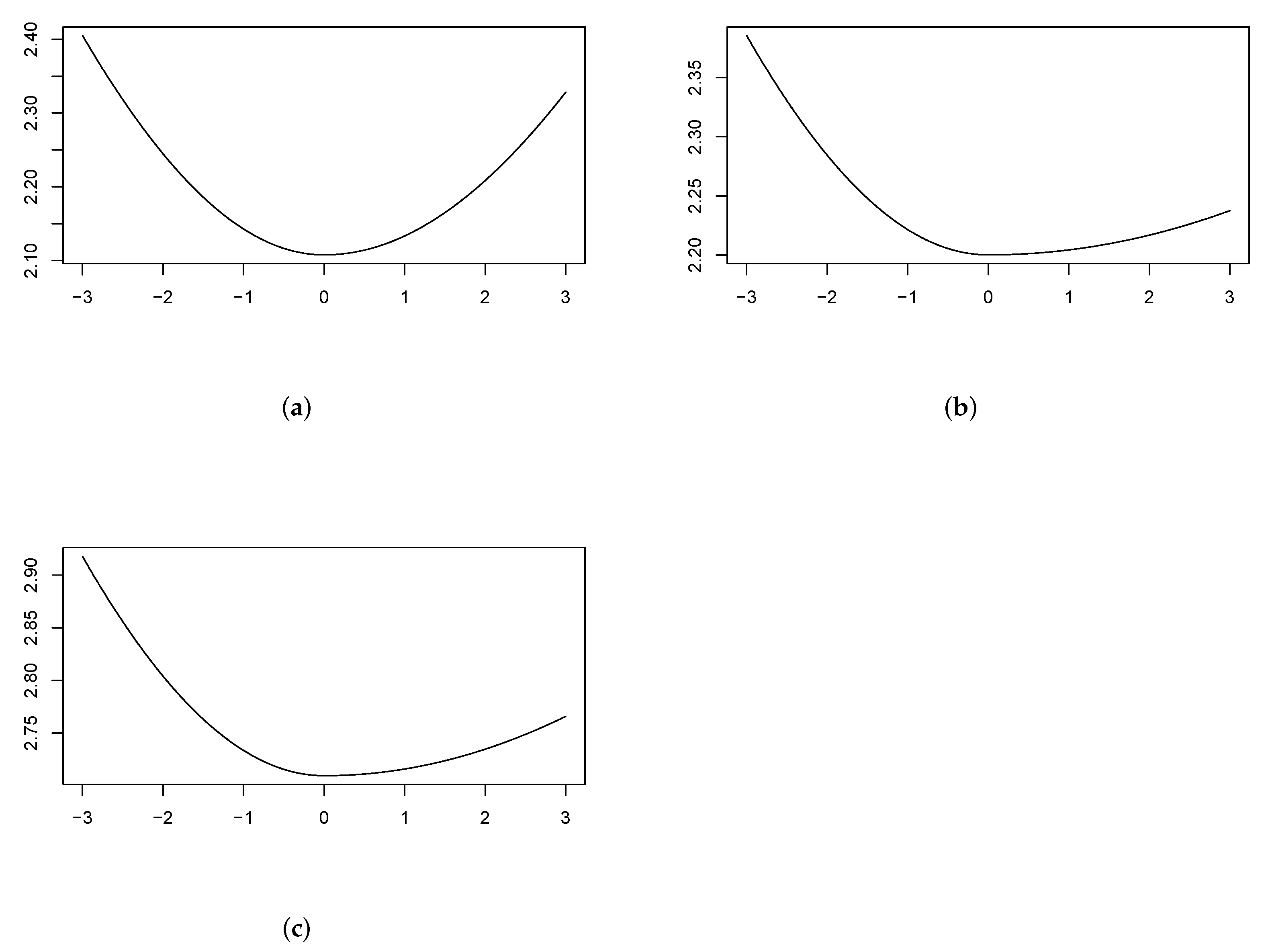
where $h_t$ is set to the sample variance of the returns, and ${\eta }_t$ ranges from −3 to 3, which covers 99.7% of the Gaussian distributed shocks. The results of INE, BRE and WTI are plotted in Figure 3.

From Figure 3, we observe that when ${\eta }_t=0$, the starting influence ranges from 2.1 (INE) to 2.2 (BRE) and 2.7 (WTI). With ${\eta }_t$ being more negative, the accelerations of the three curves are much similar. When ${\eta }_t$ reaches −3, the news impact curve increases to 2.4 for INE and BRE and 2.9 for WTI. As for the positive news, the increase in slopes is much faster for INE than for BRE and WTI. This is consistent with the observed smaller relative asymmetric effect of INE than those of BRE and WTI, as discussed above. When ${\eta }_t$ is 3, the news impact varies from around 2.35 for INE, 2.25 for BRE and 2.75 for WTI.

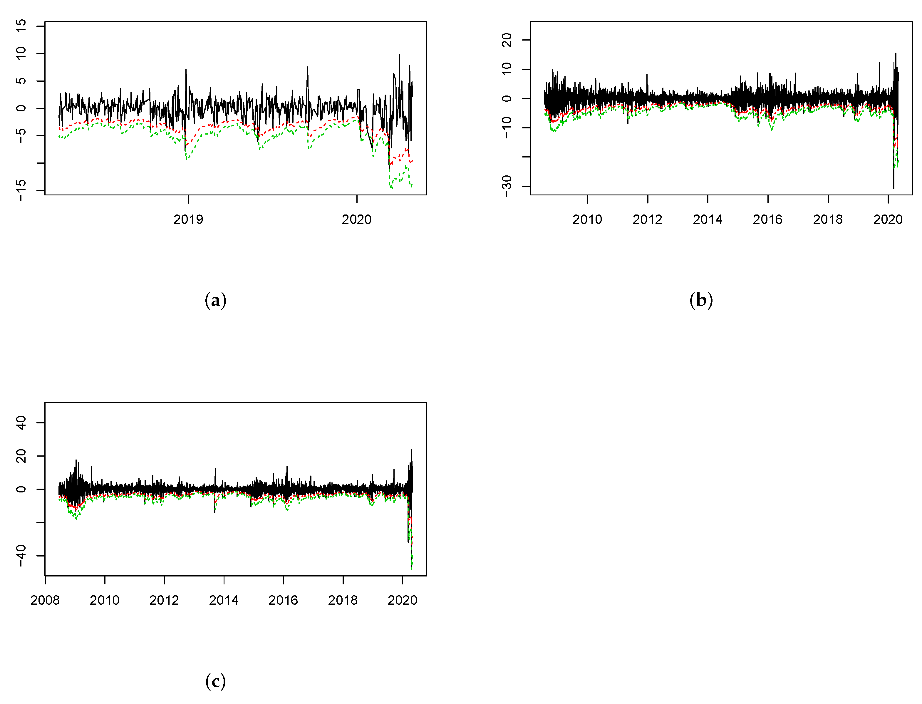
The second application considered here is the popular VaR analysis. We calculate both the 95% and 99% VaRs using the fitted conditional volatilities of TZD-GARCH for INE, BRE and WTI. More specifically, the 95% (99%) VaR at time t is the estimated ${\widehat{\sigma }}_t$ times −1.96 (−2.33). We plot the results in Figure 4, together with the demeaned daily returns. Overall, the VaRs well capture the temporal patterns of volatilities in all cases. When counting the percentages of observations that exceed the 95% VaR and 99% VaRs, the results are 6.4% and 1.2% for INE, 4.7% and 1.8% for BRE and 4.9% and 1.7% for WTI. It is also worth mentioning that the negative daily return of INE does not exceed the estimated 95% VaR on 20 April 2020, the date of the crash in WTI. Consequently, even with a Gaussian distribution, the resulting VaRs of the TZD-GARCH are satisfactorily accurate for all the three oil future volatilities.

5. Discussion

Our empirical results, especially those in Section 4.3, demonstrate implications that are of key importance for both policymakers and investors. First, consistent with the estimated strong asymmetric effects, the news impact curve indicates the importance to monitor the negative news on the oil markets. This is especially critical for the BRE and WTI, since the asymmetric effect is stronger than that of INE. For policymakers to hedge the risks of oil future movements to the macro-economy, this suggests that an uneven allocation of scarce resource should be made for the positive and negative shocks. Specifically, comparatively more resource should be distributed to monitor the arrival of negative shocks to the market to achieve the best hedging effectiveness.

In addition, the relatively more important role of negative news for BRE and WTI may be explained by their much larger trading volumes and liquidities than those of the INE. Thus, when negative news of crude oil is received, prices of BRE and WTI will respond faster with more volatilities. For policymakers and market participants, this might indicate the less market efficiency of INE, compared to BRE and WTI for the crude oil future. A quantitative comparison of this will involve the price discovery and information share [23], which remains for future works. Nevertheless, relevant trading limitations/conditions of INE may need to be redesigned by the policymaker to improve its market efficiency to attract more investors.

Last but not least, our results suggest that performing the VaR analyses with TZD-GARCH can assist policymakers and market traders in constructing accurate risk measures and other risk/portfolio management applications. For instance, studies including Van Eyden et al. [24] argue that changes in conditional volatility of crude oil could indicate recession in the economic growth globally. Further, as suggested by research such as Bampinas and Panagiotidis [25], the share of crude oil future has steadily increased in various global hedge funds, pension funds, and insurance companies, as alternative assets of safe heaven. Understanding the tail risks of crude oil futures using VaR and the proposed TZD-GARCH model would therefore be critical to the effectiveness of portfolio management. This is particularly important in the response of accelerated uncertainty over recent periods, especially after the pandemic caused by COVID-19.

6. Conclusions

This paper proposes a threshold zero-drift GARCH (TZD-GARCH) model to study and forecast the potentially non-stationary volatility of oil futures. Nesting the recent ZD-GARCH model [13] as a special case, the new TZD-GARCH model can incorporate the asymmetric influence of positive and negative news on the conditional variance. The key conclusions of this paper are summarized below. First, for the three examined crude oil futures, the INE returns over 2018–2020, and the BRE and WTI returns over 2018–2020, 2016–2020 and 2008–2020, the significant non-stationarity (stability) is evidenced by GARCH and T-GARCH (ZD-GARCH and TZD-GARCH) models. This is consistent with the empirical observations, as all three oil futures have demonstrated explosive volatilities over early-2020, which, however, is not expected to last long from a practical perspective. Second, the TZD-GARCH model almost uniformly beats the GARCH, T-GARCH and ZD-GARCH models for volatility modelling and forecasting. This is robust across various forecasting performance valuation criteria/test, oil future products, model diagnostics and sample periods. Finally, practical applications such as the Value-at-Risk analyses can be performed with the TZD-GARCH model for both policy makers and oil market participants for market monitoring and risk management purposes.

The limitation of this research is in the employed univariate methodological framework. To address this, there are two potential future directions to extend this paper. First, as examined in Chang et al. [6] and Marchese et al. [11], multivariate GARCH-type models are employed to study multiple oil futures simultaneously. From a technical point of view, it is worth extending the current univariate ZD-GARCH-type framework to be multivariate, which enables the empirical analyses such as the existence of volatility spillovers. Second, as shown in Section 4, the role of negative news is much less important for INE than those for BRE and WTI. This might be due to the slower response speed of INE with respect to the market news. Future works may consider quantitative comparison of this speed, which could adopt the price discovery method and information share [23].

References

- Tang, K.; Xiong, W. Index investment and the financialization of commodities. Financ. Anal. J. 2012, 68, 54–74. [Google Scholar] [CrossRef]
- Sadorsky, P. Modeling volatility and correlations between emerging market stock prices and the prices of copper, oil and wheat. Energy Econ. 2014, 43, 72–81. [Google Scholar] [CrossRef]
- Lv, F.; Yang, C.; Fang, L. Do the crude oil futures of the Shanghai International Energy Exchange improve asset allocation of Chinese petrochemical-related stocks? Int. Rev. Financ. Anal. 2020, 71, 101537. [Google Scholar] [CrossRef]
- Yang, D.; Zhang, Q. Drift-independent volatility estimation based on high, low, open, and close prices. J. Bus. 2000, 73, 477–492. [Google Scholar] [CrossRef] [Green Version]
- Bollerslev, T. Generalized autoregressive conditional heteroskedasticity. J. Econom. 1986, 31, 307–327. [Google Scholar] [CrossRef] [Green Version]
- Chang, C.L.; McAleer, M.; Tansuchat, R. Crude oil hedging strategies using dynamic multivariate GARCH. Energy Econ. 2011, 33, 912–923. [Google Scholar] [CrossRef] [Green Version]
- Hou, A.; Suardi, S. A nonparametric GARCH model of crude oil price return volatility. Energy Econ. 2012, 34, 618–626. [Google Scholar] [CrossRef]
- Basher, S.A.; Sadorsky, P. Hedging emerging market stock prices with oil, gold, VIX, and bonds: A comparison between DCC, ADCC and GO-GARCH. Energy Econ. 2016, 54, 235–247. [Google Scholar] [CrossRef] [Green Version]
- Hou, Y.; Li, S.; Wen, F. Time-varying volatility spillover between Chinese fuel oil and stock index futures markets based on a DCC-GARCH model with a semi-nonparametric approach. Energy Econ. 2019, 83, 119–143. [Google Scholar] [CrossRef]
- Lin, Y.; Xiao, Y.; Li, F. Forecasting crude oil price volatility via a HM-EGARCH model. Energy Econ. 2020, 87, 104693. [Google Scholar] [CrossRef]
- Marchese, M.; Kyriakou, I.; Tamvakis, M.; Di Iorio, F. Forecasting crude oil and refined products volatilities and correlations: New evidence from fractionally integrated multivariate GARCH models. Energy Econ. 2020, 88, 104757. [Google Scholar] [CrossRef]
- Francq, C.; Zakoïan, J.M. Strict stationarity testing and estimation of explosive and stationary generalized autoregressive conditional heteroscedasticity models. Econometrica 2012, 80, 821–861. [Google Scholar]
- Li, D.; Zhang, X.; Zhu, K.; Ling, S. The ZD-GARCH model: A new way to study heteroscedasticity. J. Econom. 2018, 202, 1–17. [Google Scholar] [CrossRef] [Green Version]
- Engle, R.F. Long-term skewness and systemic risk. J. Financ. Econom. 2011, 9, 437–468. [Google Scholar] [CrossRef]
- Nomikos, N.; Andriosopoulos, K. Modelling energy spot prices: Empirical evidence from NYMEX. Energy Econ. 2012, 34, 1153–1169. [Google Scholar] [CrossRef]
- Žikeš, F.; Baruník, J. Semi-parametric conditional quantile models for financial returns and realized volatility. J. Financ. Econom. 2015, 14, 185–226. [Google Scholar] [CrossRef] [Green Version]
- Glosten, L.R.; Jagannathan, R.; Runkle, D.E. On the relation between the expected value and the volatility of the nominal excess return on stocks. J. Financ. 1993, 48, 1779–1801. [Google Scholar] [CrossRef]
- Zakoian, J.M. Threshold heteroskedastic models. J. Econ. Dyn. Control 1994, 18, 931–955. [Google Scholar] [CrossRef]
- Diebold, F.X.; Mariano, R.S. Comparing predictive accuracy. J. Bus. Econ. Stat. 2002, 20, 134–144. [Google Scholar] [CrossRef]
- Bougerol, P.; Picard, N. Stationarity of GARCH processes and of some nonnegative time series. J. Econom. 1992, 52, 115–127. [Google Scholar] [CrossRef]
- Li, W.; Mak, T. On the squared residual autocorrelations in non-linear time series with conditional heteroskedasticity. J. Time Ser. Anal. 1994, 15, 627–636. [Google Scholar] [CrossRef]
- Engle, R.F.; Ng, V.K. Measuring and testing the impact of news on volatility. J. Financ. 1993, 48, 1749–1778. [Google Scholar] [CrossRef]
- Hasbrouck, J. One security, many markets: Determining the contributions to price discovery. J. Financ. 1995, 50, 1175–1199. [Google Scholar] [CrossRef]
- Van Eyden, R.; Difeto, M.; Gupta, R.; Wohar, M.E. Oil price volatility and economic growth: Evidence from advanced economies using more than a century’s data. Appl. Energy 2019, 233, 612–621. [Google Scholar] [CrossRef] [Green Version]
- Bampinas, G.; Panagiotidis, T. Oil and stock markets before and after financial crises: A local Gaussian correlation approach. J. Futur. Mark. 2017, 37, 1179–1204. [Google Scholar] [CrossRef]
Figure 1.
Volatility of INE and associated ACFs. (a) Volatility. (b) ACFs. Note: this figure presents the estimated volatility of the INE returns from the period 2018–2020 via the Yang and Zhang [4] method. The associated ACFs of the volatility are also reported.
Figure 2.
Volatility of BRE and WTI: 2008–2020. (a) BRE. (b) WTI. Note: this figure presents the estimated volatility of the BRE and WTI returns over 2008–2020 via the Yang and Zhang [4] method.
Figure 3.
News impact curves. (a) INE. (b) BRE. (c) WTI. Note: this figure presents the fitted news impact curves of INE, BRE and WTI via the TZD-GARCH model. The sample ranges from 2018 to 2020 for INE, and from 2008 to 2020 for BRE and WTI.
Figure 4.
Value-at-Risk analyses. (a) INE. (b) BRE. (c) WTI. Note: this figure presents the Value-at-Risk results of INE, BRE and WTI via the TZD-GARCH model. The sample ranges from 2018 to 2020 for INE, and from 2008 to 2020 for BRE and WTI. Dashed red and dashed green curves are the fitted 95% and 99% Value-at-Risk, respectively.