Energy Management of Refrigeration Systems with Thermal Energy Storage Based on Non-Linear Model Predictive Control

Abstract

This work addresses the energy management of a combined system consisting of a refrigeration cycle and a thermal energy storage tank based on phase change materials. The storage tank is used as a cold-energy buffer, thus decoupling cooling demand and production, which leads to cost reduction and satisfaction of peak demand that would be infeasible for the original cycle. A layered scheduling and control strategy is proposed, where a non-linear predictive scheduler computes the references of the main powers involved (storage tank charging/discharging powers and direct cooling production), while a low-level controller ensures that the requested powers are actually achieved. A simplified model retaining the dominant dynamics is proposed as the prediction model for the scheduler. Economic, efficiency, and feasibility criteria are considered, seeking operating cost reduction while ensuring demand satisfaction. The performance of the proposed strategy for the system with energy storage is compared in simulation with that of a cycle without energy storage, where the former is shown to satisfy challenging demands while reducing the operating cost by up to 28%. The proposed approach also shows suitable robustness when significant uncertainty in the prediction model is considered.

1. Introduction

Vapour-compression refrigeration systems represent the most used technique worldwide to provide cooling power, including freezing, cooling, and air conditioning applications. The amount of energy involved in such processes is huge, both for industrial and commercial/residential purposes [1]. It is reported that up to 30% of total energy needs around the world are due to Heating, Ventilating, and Air Conditioning (HVAC) systems, among which refrigeration processes represent a significant share [2].

Energy efficiency of current mechanical compression refrigeration systems has been highly improved over time, while their environmental impact has been reduced due to diverse factors. Firstly, more effective design of heat exchangers, variable-speed compressors, and electronic expansion valves (EEV) have improved heat transfer efficiency and controllability. Secondly, more efficient control strategies have been applied to satisfy cooling demand while rejecting disturbances and achieving the highest energy efficiency possible with a direct environmental impact. For instance, Jain and Alleyne developed a model predictive controller using a dynamic exergy-based objective function to maximize exergetic efficiency of a basic refrigeration cycle [3]. Concerning HVAC systems in buildings, Espejel-Blanco et al. have recently presented an HVAC temperature control system based on the Predicted Mean Vote (PMV) index calculation, which combines the values of humidity and temperature to define comfort zones and achieves energy savings ranging from 33% to 44% against the built-in control of the HVAC equipment [4]. Kou et al. develop both model-based and data-driven HVAC control strategies to determine the optimal control actions for HVAC systems, highlighting a significant trade-off between electricity costs and computational speed between both strategies [5]. Furthermore, Macieira et al. have also presented an energy management model for HVAC control based on reinforcement learning, to manage the HVAC units in smart buildings according to the prediction of users, current environmental context, and current energy prices [6].

In recent years, a novel line of research regarding cold-energy management has been introduced which involves the addition of thermal energy storage (TES) systems to the standard refrigeration cycle. Accordingly, cooling production and demand can be decoupled, since excess cold energy may be stored in the TES system, being released when required, as common storage strategies applied to solar plants [7]. This setup makes it possible to use lower capacity systems, since they need not be oversized to face peak-demand periods [8], and thus the investment cost may be reduced. Moreover, the cycle may be operated in more favourable terms, which improves efficiency and reduces energy usage. Furthermore, it is possible to schedule the cooling production according to the variable cost of electricity given by the energy market. Thus, an optimal strategy (peak-shifting) would be to produce as much cold energy as possible during the low-priced periods, while storing the excess in the TES system, and to produce as little as possible during the high-priced periods, releasing the cold energy previously stored [9].

Concerning the design of the storage system, most commercial and developing systems rely on phase change materials (PCM) [10]. The main reason is that their thermodynamic properties are more suitable for energy storage than those of sensible-heat materials [11]. PCM are able to store larger amount of energy per unit volume and their temperature remains approximately constant in latent state, which improves heat transfer efficiency. Concerning domestic refrigerators, Bista et al. published a thorough review [12], regarding PCM selection and placement inside the refrigerator, where the use of PCM is shown to increase the Coefficient of Performance (COP) with a relatively significant margin. Among the PCM-based systems, there are several factors defining the storage configuration, such as the PCM encapsulation and the heat exchanger layout where the PCM and the heat transfer fluid (HTF) meet, the packed bed technology being one of the most used configurations [13]. Regarding the latter, Berdja et al. proposed a novel approach to optimize the dimensions of the packed bed heat exchanger, according to the technical features and operating conditions of a standard refrigerator [14].

Many works in the literature have addressed cold-energy management of refrigeration systems with energy storage. For instance, three works by Wang et al. cover the design [15], modelling [16], and control [17] of a large-scale HVAC plant, where a ring of PCM-based TES tanks acts as a cold-energy reservoir. Control policies are proposed to activate/deactivate the TES tanks, seeking high performance. Other works implement management strategies based on exergy analysis, where a combined use of the different PCM modules is applied [18]. Furthermore, model predictive control (MPC) also represents a successful strategy. Indeed, it has been applied for HVAC without energy storage [19,20], but the potential of predictive strategies for TES-backed-up systems is much higher. For instance, Shafiei et al. [21] propose a MPC framework to minimize the divergence in electric energy usage with respect to a given reference, in a large-scale refrigeration plant. For that purpose, energy collected by and retrieved from the TES is estimated, and an optimization problem is formulated by introducing the reference of the evaporation temperature as a virtual control variable. Shafiei et al. [22] also apply predictive control to TES-backed-up refrigerated freight transport, where the TES tank is embedded in parallel with the refrigeration cycle. The prescribed delivery route profile, along with traffic and environmental information, are incorporated into the algorithm to predict the cooling demand. Furthermore, Schalbart et al. present an MPC strategy to the management of an ice-cream warehouse refrigeration system coupled to a TES tank [23]. The controller is based on a steady-state refrigeration cycle model and energy balances on the TES tank and the warehouse.

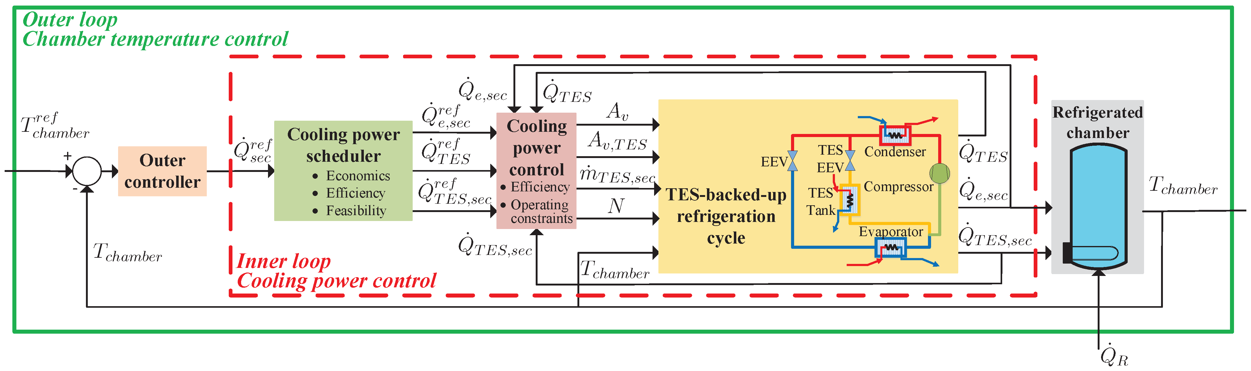
In this work, a novel hybrid configuration, that comprises a PCM-based TES tank especially designed to complement an existing refrigeration system, is analysed from the point of view of energy management. The layout, shown in Figure 1, is slightly different to that usually applied in the aforementioned works, due to the features of the original refrigeration facility.

As depicted in Figure 1, the fluid to be cooled (hereinafter referred to as secondary fluid) is pumped from a tank, which represents the refrigerated chamber, both to the evaporator and to the TES tank, and it is then recirculated to the chamber. An electric resistance is used at this tank to produce heat and simulate the cooling demand, which must be satisfied by both secondary fluid streams. The vapour-compression cycle transfers cold energy to the evaporator by cooling the secondary fluid, but the refrigerant also circulates through the TES tank while charging it, being the latter the cold HTF in this case. The secondary fluid also circulates through the TES tank while discharging it, and thus the warm HTF does not match the cold HTF, as a very relevant difference with respect to the packed bed technology. The layout of the TES tank comprises a number of PCM cylinders and two bundles of pipes, one corresponding to the refrigerant and the other to the secondary fluid, all of them bathed in the so-called intermediate fluid. This TES setup is very similar to that described in a recent work by Bejarano et al. [24], the PCM encapsulation being the only relevant difference. To the authors’ knowledge, this setup is novel and the cold-energy management and economic potential offered to industrial refrigeration facilities is first analysed in this work, which represents one of the main contributions of the article. This configuration involves several operating modes, according to the manipulation of the expansion valves and pumps, that enable/disable the different fluid streams and make the system hybrid, in addition to its inherent non-linear features.

As previously mentioned, cold-energy storage allows decoupling of cooling demand and production. Moreover, given the parallel arrangement between the evaporator and the TES tank, the cooling demand at the refrigerated chamber may be satisfied using both secondary fluid streams. It implies that the TES-backed-up refrigeration system is able to satisfy peak cooling demand that might be infeasible for the original standard refrigeration cycle, due to the double contribution provided by both secondary fluid streams. The economic and feasibility potential offered by the addition of the TES tank to the original refrigeration cycle is explored by proposing a scheduling and control strategy based on non-linear MPC to satisfy the cooling demand while minimizing the daily operating cost.

The main contribution of this work regarding the scheduling is the application of non-linear model predictive control (NMPC) to this hybrid system, where the computational cost of the prediction model is also considered. A non-linear model describing the dominant dynamics of the TES tank is proposed to be used as the prediction model. The latter is developed from the frequency analysis performed in the work by Rodríguez et al. [25], where it is stated that two very different time scales arise in the combined system: one related to the fastest dynamics of the refrigeration cycle, and another, slower one, related to heat transfer within the TES tank. In that work, a detailed model of the TES-backed-up refrigeration cycle was presented, focusing on the faster dynamics caused by the refrigerant circulation, which must be integrated using a small sampling time, in the order of a few seconds. However, such complexity is not affordable or even necessary when addressing the scheduling stage, according to the desired sampling time of several minutes, given the slower dynamics related to heat transfer within the TES tank. Therefore, in this work a simplified non-linear model is proposed, focusing on the dominant dynamics related to the TES tank, which turns out to be far from trivial but more suitable to model-based predictive strategies, especially concerning computational load. This is one of the main contributions of the work, since the reduced computational cost of the prediction model allows direct application of a non-linear model predictive control strategy while ensuring reasonable computation times. The performance of the proposed scheduler for the TES-backed-up system is compared in simulation with the refrigeration cycle without energy storage, while an analysis on the operating cost and constraint meeting is also performed, even when considering significant parametric uncertainty in the prediction model.

Therefore, the main contributions of the work are summarised below:

• A novel setup of a TES-backed-up refrigeration system is presented, where the TES tank is inserted within the refrigeration cycle, causing the heat transfer fluid to differ between charging and discharging processes. This is an essential and relevant difference with respect to the dominant packed bed technology [13,14].
• A layered NMPC-based scheduling and control strategy is applied to the TES-backed-up refrigeration system, which explores the economic and feasibility potential of such a setup, where the control of the compressor and expansion valves is directly affected by the embedding of the TES tank within the refrigeration cycle, in contrast with the packed bed technology, where the refrigerant circulation is not affected by the state of the storage tank [13]. Thus, the existing control strategies previously detailed [17,18,21,22,23] cannot be applied to the configuration under study.
• A simplified and computationally efficient non-linear prediction model describing the dominant dynamics of the system is presented, which allows the application of the previously mentioned non-linear predictive strategy with reasonable computational load, when compared with the accurate but computationally expensive existing dynamic model [25].

The work is organised as follows. Section 2 describes the main characteristics of the designed TES tank and its embedding in the existing facility. Section 3 addresses the modelling of the combined system, focusing on the dominant dynamics related to heat transfer within the TES tank. The overall control strategy is presented in Section 4, focusing on the NMPC-based scheduling algorithm. Section 5 describes a case study for a demanding load profile, where the need for operating mode scheduling is justified according to the power constraints. The economic performance and demand satisfaction of the scheduling strategy are compared to that of the original cycle without energy storage in simulation. Finally, Section 6 summarises the main conclusions and some future work is proposed.

2. Combined System Description

2.1. Terminology

All abbreviations, symbols, and subscripts/superscripts used in the work are detailed in

Table 1. Abbreviations, symbols, and subscript/superscript notation.

Italic Symbols			Subscripts
Symbol	Description	Units	Symbol	Description
A	Opening	%	$chamber$	refrigerated chamber
$CAPEX$	Capital Expenditure	€	$coat$	coating
$COP$	Coefficient of Performance	–	$cost$	economic cost
$c_p$	Specific heat at constant pressure	J kg−1 K−1	e	evaporator
D	Diameter	m	$in$	inlet/input
$EEV$	Electronic Expansion Valve	–	$int$	intermediate fluid
e	Thickness	m	$lay$	cylindrical layer
g	Non-linear dynamic model of the TES tank	–	$out$	outlet/output
$HVAC$	Heating, Ventilating, and Air Conditioning	–	$pcm$	PCM
$HTF$	Heat Transfer Fluid	–	R	electric resistance
h	Specific enthalpy	J kg−1	$ratio$	related to the charge ratio
J	Objective function	–	$refr$	refrigerant
k	Discrete step time	–	$SH$	superheating
L	Length	m	$sec$	secondary fluid
$MPC$	Model Predictive Control	–	$surr$	surroundings
$\dot{m}$	Mass flow rate	kg s−1	$tank$	tank
m	Mass	kg	$TES$	Thermal Energy Storage
N	Compressor speed	Hz	v	expansion valve
$NMPC$	Non-linear Model Predictive Control	–	Superscripts
n	Number of elements	–	$cond$	thermal conduction
P	Pressure	Pa	$conv$	convection
$PCM$	Phase Change Material	–	$ext$	external
$PH$	Prediction horizon	–	$lat$	latent state
$\dot{Q}$	Cooling power	W	$lat+$	maximum latency point
R	Thermal resistance	K W−1	$lat-$	minimum latency point
T	Temperature	K	$max$	maximum
$TES$	Thermal Energy Storage	–	$min$	minimum
t	Time	h	$ref$	reference
U	Internal energy	J	$uncer$	uncertain
V	Volume	m3	$wall$	wall
w	Weight in the objective function	€ MWh−1
x	State vector	–
Greek Symbols
$\alpha$	Coefficient of thermal losses	W m−2 K−1
$\gamma$	Charge ratio	–
$\kappa$	Thermal conductivity	W m−1 K−1
$\rho$	Density	kg m−3

. The CoolProp tool [26] has been used to compute the thermodynamic properties of all involved fluids.

2.2. TES Tank Embedding

The designed TES tank is intended to complement a two-compression-stage, two-load-demand experimental refrigeration facility located at the Department of Systems Engineering and Automatic Control at the University of Seville (Spain) [25,27], which works with R404a as refrigerant and a 60% in volume propylene glycol aqueous solution as the secondary fluid. The models and parameters of the refrigeration cycle elements are described in detail in [28]. Figure 2 shows only a section of this facility, including a one-stage, one-load-demand refrigeration cycle where the TES tank is arranged in parallel with the evaporator.

Two bundles of pipes run through the TES tank, corresponding to the refrigerant and the secondary fluid, respectively. An additional expansion valve is added to drive the refrigerant from the condenser (labelled as TES EEV in Figure 2), whereas an additional pump is needed to impulse the secondary fluid from the refrigerated chamber (labelled as TES Pump). Notice that the elements defined in [28] as the main compressor, the air condenser, the evaporator related to the refrigerated chamber at −20 °C, and the corresponding expansion valve EEV2 are considered in this configuration, whereas the TES EEV is assumed to be identical to EEV2. Further technical details about the embedding of the TES tank are described in [24].

2.3. TES Tank Configuration

The TES tank setup is shown in Figure 3, where the relevant inputs, outputs, and states are highlighted. A number of steel cylinders enclose the PCM, while two bundles of pipes distribute the refrigerant and secondary fluid streams in a counter-current configuration, in such a way that homogeneous heat transfer is achieved. The intermediate fluid (featuring high thermal conductivity and low heat capacity) bathes all cylinders and pipes to homogenise heat transfer.

The physical and thermodynamic parameters of the TES tank are included in

Table 2. Design parameters of the TES tank.

Symbol	Description	Value	Units
$L_{tank}$	Length of the TES tank	1.4	m
$D_{tank}$	Internal diameter of the TES tank	0.4	m
$e_{tank}$	Thickness of the TES tank wall	0.005	m
$n_{pcm}$	Number of PCM cylinders	17	–
$D_{pcm}$	External diameter of the PCM cylinders	0.0445	m
$e_{pcm}$	Thickness of the PCM cylinder coating	0.001	m
${\kappa }_{coat,pcm}$	Thermal conductivity of the PCM cylinder coating	16.3	W m−1 K−1
$n_{refr}$	Number of refrigerant pipes	36	–
$D_{refr}$	External diameter of the refrigerant pipes	0.020	m
$e_{refr}$	Thickness of the refrigerant pipe wall	0.001	m
${\kappa }_{coat,refr}$	Thermal conductivity of the refrigerant pipe wall	16.3	W m−1 K−1
$n_{sec}$	Number of secondary fluid pipes	32	–
$D_{sec}$	External diameter of the secondary fluid pipes	0.020	m
$e_{sec}$	Thickness of the secondary fluid pipe wall	0.001	m
${\kappa }_{coat,sec}$	Thermal conductivity of the secondary fluid pipe wall	16.3	W m−1 K−1
$V_{TES,int}$	Volume of the intermediate fluid	0.109	m3
${\alpha }_{surr}$	Coefficient of thermal losses	0.1	W m−2 K−1

, while the thermodynamic properties of the PCM are shown in

Table 3. Phase change material properties.

Symbol	Description	Value	Units
${c_p}_{pcm}$	Specific heat at constant pressure	3690	J kg−1 K−1
$h_{pcm}^{lat}$	Specific enthalpy of fusion (latent phase)	222,000	J kg−1
$T_{pcm}^{lat}$	Phase change temperature	−29	°C
${\kappa }_{pcm}$	Thermal conductivity	0.64	W m−1 K−1
${\rho }_{pcm}$	Density	1420	kg m−3

. The intermediate fluid is a 60% in volume ethylene glycol aqueous solution featuring high thermal conductivity.

Regarding the inputs, the description of the inlet flows includes extensive (${\dot{m}}_{TES}$ and ${\dot{m}}_{TES,sec}$) and intensive variables (the {$P_{TES,in}$ – $h_{TES,in}$} pair for the refrigerant and $T_{TES,sec,in}$ for the secondary fluid). The latter describe the thermodynamic state of the corresponding fluid, whereas the surroundings temperature $T_{surr}$ represents a measurable disturbance. Concerning the outputs, the thermodynamic state of the outlet flows is determined by $T_{TES,sec,out}$ and the {$P_{TES,out}-h_{TES,out}$} pair. The variables ${\dot{Q}}_{TES}$ and ${\dot{Q}}_{TES,sec}$ refer to the cooling powers transferred between the refrigerant/secondary fluid and the intermediate fluid. The TES tank state vector $x_{TES}$ is made up of the temperature of the intermediate fluid $T_{int}$ and an enthalpy description of the cold energy stored inside every PCM cylinder. Notice that the cold-energy storage ratio ${\gamma }_{TES}$ (also called as charge ratio) is not actually a state variable, since it can be computed from the cold-energy distribution of the PCM cylinders.

3. Modelling

3.1. Simplified Dynamic Modelling

In this section a simplified dynamic model describing the dominant plant dynamics as straightforwardly as possible is intended to be developed, so that it can be used as the prediction model in the cooling power scheduling strategy. It is to be noted that the simplified model is used only for the sake of scheduling, while the plant is simulated using the detailed and more realistic model described in [25].

In that work, it was shown that two different time scales arise in the combined system, one related to the faster intrinsic dynamics of the refrigeration cycle, and a slower one related to the states of the TES tank. Indeed, since it is the intermediate fluid that transfers heat to the refrigerant pipes, the secondary fluid pipes, and the PCM cylinders, its low heat capacity is the main cause of those slower dynamics. A detailed model of the combined system, focused on the fastest dynamics caused by the refrigerant circulation, was proposed in [25]. That model also describes the slower dynamics related to heat transfer within the TES tank, but the sampling time needed to be small enough to properly describe the refrigerant dynamics.

Since the scheduling strategy is intended to be performed using a much greater sampling time that fits the dynamics of the cooling demand profile and the TES tank, such a detailed model becomes unsuitable and computationally unaffordable for the scheduling strategy. Therefore, in this work we are interested in developing a simplified version of the previous detailed model, focusing on the thermal behaviour of the intermediate fluid and the energy distribution of the PCM cylinders, that are indeed the slow TES states of the detailed model.

Concerning the slower time scale, since the refrigeration cycle intrinsic dynamics become negligible, the whole TES-backed-up vapour-compression cycle can be statically modelled. Then, the intermediate fluid and its heat transfer to the PCM cylinders represent the dominant dynamics. As a consequence, in the simplified model, the TES tank charging ${\dot{Q}}_{TES}$ and discharging ${\dot{Q}}_{TES,sec}$ cooling powers are considered as virtual manipulated inputs, whereas the refrigeration cycle is implicit and supposed to somehow provide these cooling powers, within some feasible ranges. The simplified model is schematically described in Figure 4, where the surroundings temperature $T_{surr}$ is considered as a measurable disturbance.

Then, the simplified model just describes the non-linear dynamics of the intermediate fluid and its heat transfer to the PCM cylinders. The highly time-efficient dynamic modelling approach proposed in [29] is applied, due to the high speed requirements imposed by the predictive scheduler, since the model is expected to run countless times over a certain horizon within the optimization procedure.

In the modelling approach presented in [29], the PCM elements (in this case, cylinders) are divided into a certain number of layers $n_{lay}$, each one of them featuring the same mass $m_{lay}$. The number of considered layers represents a trade-off between accuracy and computational load. Some assumptions have been made to develop the time-efficient discrete model. On the one hand, the intrinsic dynamics of the layers in the sensible zone are assumed to be negligible, thus their temperatures are computed according to a steady-state thermal conduction model. On the other hand, cold energy is considered to be transferred at constant rate, provided that the set of layers in latent and sensible zone does not vary.

As mentioned above, the TES tank state vector $x_{TES}$ is made up of the temperature of the intermediate fluid $T_{int}$ and an enthalpy description of the cold energy stored inside every PCM cylinder, which may be defined as indicated in Equation (1):

$$x_{TES}=\left[\begin{array}{c}{h}_{pcm,1}\\ h_{pcm,2}\\ \cdots \\ h_{pcm,n_{lay}}\\ T_{int}\end{array}\right]\in {\mathbb{R}}^{n_{lay}+1},$$

(1)

where the specific enthalpies $h_{pcm,j}\forall j=1,...,n_{lay}$ of all the cylindrical layers are included in the state vector. The description of the recursive algorithm implementing the simplified dynamic model of the TES tank, given the TES tank charging ${\dot{Q}}_{TES}$ and discharging ${\dot{Q}}_{TES,sec}$ cooling powers as virtual manipulated inputs and the surroundings temperature $T_{surr}$ as a measurable disturbance, is given in a step-by-step sketch, similarly to the original time-efficient discrete model described in [29]:

1.

From a given state vector $x_{TES}\left(t\right)$, an inward scanning sequence of the PCM layers is performed, looking for the first layer $j_0$ in latent zone, as indicated in Equation (2):

$$j_0=max\left\{j\in \{1,\dots n_{lay}\}\mid h_{pcm}^{lat-}\le h_{pcm,j}\left(t\right)\le h_{pcm}^{lat+}\right\}.$$

(2)

2.

The thermal resistance $R_{pcm,j_0}^{cond}$, corresponding to the spherical shell including all PCM layers exterior to layer $j_0$: $j\in \{j_0+1,\dots ,n_{lay}\}$, is computed as if it was a single, clustered thermal-conduction layer.

3.

The cooling power transferred between the intermediate fluid and $j_0$ layer is computed as shown in Equation (3):

$${\dot{Q}}_{pcm,j_0}\left(t\right)={\displaystyle \frac{T_{int}\left(t\right)-T_{pcm,j_0}\left(t\right)}{R_{pcm,j_0}^{cond}+R_{pcm}^{cond,wall}+R_{pcm}^{conv,ext}}},$$

(3)

where $R_{pcm}^{cond,wall}$ refers to the thermal conduction resistance due to the PCM cylinder coating, and $R_{pcm}^{conv,ext}$ represents the thermal resistance caused by external natural convection with the intermediate fluid.

4.

Layer $j_0$ is initially considered to remain in latent zone during the complete time period $\Delta t$, in such a way that cold energy is assumed to be transferred at the constant rate ${\dot{Q}}_{pcm,j_0}\left(t\right)$, as shown in Equation (4):

$$\Delta U_{pcm,j_0}={\int }_t^{t+\Delta t}{\dot{Q}}_{pcm,j_0}dt\approx {\dot{Q}}_{pcm,j_0}\left(t\right)\Delta t.$$

(4)

5.

The specific enthalpy of layer $j_0$ is updated accordingly at the end of the considered time period $\Delta t$, as indicated in Equation (5):

$$h_{pcm,j_0}(t+\Delta t)=h_{pcm,j_0}\left(t\right)+{\displaystyle \frac{\Delta U_{pcm,j_0}}{m_{lay}}}.$$

(5)

6.

Having reached this point, two possibilities may arise:

• Layer $j_0$ remains in latent zone: $h_{pcm}^{lat-}\le h_{pcm,j_0}(t+\Delta t)\le h_{pcm}^{lat+}$. Therefore, the assumption made in Step 4 is confirmed and the specific enthalpy of the layers interior to $j_0$ is not affected during the time period under study, as described in Equation (6):

  $$h_{pcm,j}(t+\Delta t)=h_{pcm,j}\left(t\right)\forall j<j_0.$$

  (6)
  However, layers exterior to $j_0$ are shown to be already in the sensible zone. To compute their specific enthalpy, their temperature is first estimated as indicated in Equation (7), applying a steady-state thermal conduction model, where $R_{pcm,j}^{cond}$ for every layer j is computed in a similar way to $R_{pcm,j_0}^{cond}$ in Step 2:

  $$T_{pcm,j}(t+\Delta t)=T_{pcm,j-1}(t+\Delta t)+{\dot{Q}}_{pcm,j_0}{R}_{pcm,j}^{cond}\forall j>j_0.$$

  (7)
  Then, the specific enthalpy of the layers exterior to $j_0$ is computed at the end of the time period under study, depending on whether the layer is superheated or subcooled, as shown in Equation (8):

  $$\begin{array}{cc}\hfill h_{pcm,j}(t+\Delta t)& =h_{pcm}^{lat-}-c_{p,pcm}\left(T_{pcm}^{lat}-T_{pcm,j}(t+\Delta t)\right)\hfill \\ \hfill & \mathrm{if}j\mathrm{is}\mathrm{subcooled}\mathrm{layer},\hfill \\ \hfill h_{pcm,j}(t+\Delta t)& =h_{pcm}^{lat+}+c_{p,pcm}\left(T_{pcm,j}(t+\Delta t)-T_{pcm}^{lat}\right)\hfill \\ & \mathrm{if}j\mathrm{is}\mathrm{superheated}\mathrm{layer}.\hfill \end{array}$$

  (8)
  The cooling power that the whole PCM cylinder transfers to the intermediate fluid, ${\dot{Q}}_{pcm}\left(t\right)$, matches the cooling power transferred between the intermediate fluid and $j_0$ layer, ${\dot{Q}}_{pcm,j_0}\left(t\right)$. Eventually, the temperature of the intermediate fluid is updated using the discrete approximation given in Equation (9):

  $$\begin{array}{cc}\hfill & T_{int}(t+\Delta t)=T_{int}\left(t\right)-{\displaystyle \frac{\Delta t}{m_{int}{c}_{p,int}}}\left[{\dot{Q}}_{TES}+{\dot{Q}}_{TES,sec}+n_{pcm}{\dot{Q}}_{pcm}\left(t\right)+{\dot{Q}}_{surr}\right],\hfill \end{array}$$

  (9)

  where the following sign criteria is considered:

  −

  ${\dot{Q}}_{TES}$: Cooling power transferred from the refrigerant to the intermediate fluid (typically positive).

  −

  ${\dot{Q}}_{TES,sec}$: Cooling power transferred from the secondary fluid to the intermediate fluid (typically negative).

  −

  ${\dot{Q}}_{pcm}\left(t\right)$: Cooling power transferred from each PCM cylinder to the intermediate fluid (positive during discharging cycle, negative during charging cycle).

  −

  ${\dot{Q}}_{surr}$: Cooling power transferred from the intermediate fluid to the surroundings (typically negative). This cooling power can be easily estimated from the temperature gradient between the intermediate fluid and the surroundings and the thermal insulation features of the TES tank.

• Layer $j_0$ leaves latent zone. In other words, the latent energy of layer $j_0$ run out some time before the period under study finished, $\Delta t_{j_0}\le \Delta t$, and then the layer $j_0$ got into sensible zone. The precise instant is estimated, considering a constant rate, ${\dot{Q}}_{pcm,j_0}\left(t\right)$, and the remaining latent energy of layer $j_0$ at instant t, as shown in Equation (10) for a charging process or Equation (11) for a discharging process:

  $$\Delta t_{j_0}={\displaystyle \frac{m_{lay}(h_{pcm,j_0}\left(t\right)-h_{pcm}^{lat-})}{{\dot{Q}}_{pcm,j_0}}},$$

  (10)

  $$\Delta t_{j_0}={\displaystyle \frac{m_{lay}(h_{pcm}^{lat+}-h_{pcm,j_0}\left(t\right))}{{\dot{Q}}_{pcm,j_0}}}.$$

  (11)
  Then, a shorter time interval, $\Delta t_{j_0-1}$, can be computed as shown in Equation (12):

  $$\Delta t_{j_0-1}=\Delta t-\Delta t_{j_0}.$$

  (12)
  This time interval $\Delta t_{j_0-1}$ is used for successive estimation, in which the next inner layer, $j_0-1$, is considered as the new first layer in the latent zone, and the algorithm restarts from Step 2, but using the corresponding time period $\Delta t_{j_0-1}$, instead of $\Delta t$.
  Then, the cooling power transferred between each PCM cylinder and the intermediate fluid, ${\dot{Q}}_{pcm}$ eventually has several successive contributions along the original time period $\Delta t$, as shown in Equation (13):

  $$\begin{array}{c}\hfill {\dot{Q}}_{pcm}=\left\{{\dot{Q}}_{pcm,j_0},{\dot{Q}}_{pcm,j_0-1},\dots {\dot{Q}}_{pcm,j_0-i}\right\},\end{array}$$

  (13)
  $j_0-i$ being the most inner layer found in the latent state during the time period under study $\Delta t$. Obviously, the addition of the partial time intervals matches the complete interval, as shown in Equation (14):

  $$\sum _{l=0}^{l=i}\Delta t_{j_0-l}=\Delta t.$$

  (14)
  For each one of the partial time intervals, $T_{int}$ is updated using Equation (9), giving rise to the succession shown in Equation (15):

  $$\begin{array}{c}\hfill T_{int}(t+\Delta t_{j_0})=T_{int}(t)-{\displaystyle \frac{\Delta t_{k_0}}{m_{int}{c}_{p,int}}}\left[{\dot{Q}}_{TES}+{\dot{Q}}_{TES,sec}+n_{pcm}{\dot{Q}}_{pcm,j_0}+{\dot{Q}}_{surr}\right]\\ \hfill T_{int}(t+\sum _{l=0}^{l=1}\Delta t_{j_0-l})=T_{int}(t+\Delta t_{j_0})-{\displaystyle \frac{\Delta t_{j_0-1}}{m_{int}{c}_{p,int}}}\left[{\dot{Q}}_{TES}+{\dot{Q}}_{TES,sec}+n_{pcm}{\dot{Q}}_{pcm,j_0-1}+{\dot{Q}}_{surr}\right]\\ \hfill \cdots \\ \hfill T_{int}(t+\sum _{l=0}^{l=i}\Delta t_{j_0-l})=T_{int}(t+\sum _{l=0}^{l=i-1}\Delta t_{j_0-i})-{\displaystyle \frac{\Delta t_{j_0-i}}{m_{int}{c}_{p,int}}}\left[{\dot{Q}}_{TES}+{\dot{Q}}_{TES,sec}+n_{pcm}{\dot{Q}}_{pcm,j_0-i}+{\dot{Q}}_{surr}\right]\\ \hfill T_{int}(t+\sum _{l=0}^{l=i}\Delta t_{j_0-l})\equiv T_{int}(t+\Delta t).\end{array}$$

  (15)

The proposed model can be expressed as shown in Equation (16), where the function g stands for the complete discrete model, also shown in Figure 4:

$$x_{TES}(t+\Delta t)=g(x_{TES}\left(t\right),{\dot{Q}}_{TES}^{ref}\left(t\right),{\dot{Q}}_{TES,sec}^{ref}\left(t\right),T_{surr}\left(t\right)).$$

(16)

As stated before, since the dynamic model presented in [25] involves a small sampling time to properly describe the fastest system dynamics, it does not turn out to be suitable or even computationally affordable to be used as the prediction model within a predictive scheduling strategy. This is where the simplified dynamic model proposed in this section, which retains the dominant dynamics while allowing a much greater sampling time, comes handy. Therefore, the computational complexity of the proposed model is not compared with the one in [25] due to impracticability, but the benefits provided in terms of computational cost are evident.

3.2. Operating Modes

Diverse operating modes can be defined, according to all possible combinations of the three main cooling powers involved in the problem: the cooling power provided to the secondary fluid at the evaporator ${\dot{Q}}_{e,sec}$, the TES charging cooling power ${\dot{Q}}_{TES}$, and the TES discharging cooling power ${\dot{Q}}_{TES,sec}$ [25]. Up to eight operating modes have been defined and discussed in the aforementioned work, though the most useful operating modes might be modes 1 to 4, since modes 5 and 8 require no cooling demand, whereas modes 6 and 7 involve simultaneous TES tank charging and discharging, which may not make sense from the operating point of view. The most interesting operating modes are graphically described in Figure 5.

Mode 1 may be scheduled when the cooling demand can be satisfied by using only the refrigeration cycle and it is interesting to simultaneously charge the TES tank. Mode 2 might be scheduled in the same situation, but when the TES tank is fully charged or it is not economically interesting to continue charging it. Mode 3 is useful when the cooling demand is greater than the maximum power achievable by using only the refrigeration cycle. Mode 4 requires that the demand can be satisfied by only discharging the TES tank, thus the refrigeration cycle is stopped.

4. Scheduling and Control Strategy

4.1. Overview

Figure 6 represents the proposed scheduling and control strategy. The main objective is to track a certain reference of the chamber temperature $T_{chamber}^{ref}$, which, by means of the so-called outer controller, may result in a reference of the overall cooling power that must be provided to the secondary fluid ${\dot{Q}}_{sec}^{ref}$, since an electric resistance transfers a certain heat ${\dot{Q}}_R$ to the secondary fluid to simulate the thermal load. This controller is not addressed in this work due to its simplicity, since it tackles a single reference $T_{chamber}^{ref}$ and a single control action ${\dot{Q}}_{sec}^{ref}$. A simple PID control could be applied without difficulty, thus the development of such a control law has not been considered of interest for this work.

Given a certain demand ${\dot{Q}}_{sec}^{ref}$, the scheduler is intended to compute the references of the three cooling powers involved: ${\dot{Q}}_{e,sec}^{ref}$, ${\dot{Q}}_{TES}^{ref}$, and ${\dot{Q}}_{TES,sec}^{ref}$, according to efficiency, economic, and feasibility criteria. The cooling power controller is then responsible for getting the TES-backed-up refrigeration system to actually provide the three required cooling powers by manipulating the four manipulated variables available, namely, the compressor speed N, both expansion valve openings $A_v$ and $A_{v,TES}$, and the TES pump. In Figure 6, the secondary mass flow that circulates through the TES tank ${\dot{m}}_{TES,sec}$ is considered as a virtual manipulated variable, while the actual one is the TES pump speed/power. Anyway, for a certain required value of ${\dot{m}}_{TES,sec}$, a simple regulator is intended to drive the TES pump to actually provide the desired secondary mass flow.

Therefore, four manipulated variables are available in the cooling power control, whereas only three references must be tracked. These three set points define the desired operating mode, according to Figure 5, in such a way that if one is zero, it involves one of the extensively manipulated variables ($A_v$, $A_{v,TES}$, or ${\dot{m}}_{TES,sec}$) also being zero. However, when the refrigerant circulates through the compressor (all operating modes considered in Figure 5 except mode 4), the degree of superheating at the compressor intake $T_{SH}$ must be positive, in order to avoid mechanical breakdowns. Since the fourth manipulated variable is thus responsible for getting the degree of superheating $T_{SH}$ over a certain security limit, in this case the control problem is fully actuated.

Concerning the scheduler, given a certain cooling demand forecast, a NMPC-based strategy is applied. In view of the demand forecast and the expected energy prices throughout the day, an operating mode scheduling is proposed, and then the cooling power references are scheduled by solving a non-linear optimization problem. The simplified TES tank dynamic model proposed in Section 3.1 is used as the prediction model, since the scheduling strategy is focused on demand satisfaction and the TES tank cold-energy management, not on the actual production of the required powers, to be addressed by the cooling power controller. Nevertheless, some constraints on the scheduled powers (that turn out to be the decision variables of the optimization problem) must be imposed in order to ensure that the cooling power control problem is feasible and the references are indeed achievable. Additional constraints aimed to keep the PCM cylinders within latent zone are imposed, while the objective function of the optimization problem is based on economic and efficiency criteria.

One important issue is related to time scales. The scheduling strategy is intended to be solved with a sampling time suitable to fit the demand profile, whereas the cooling power control is intended to be performed at the baseline sampling rate, fitting the fastest dynamics related to the refrigeration cycle.

4.2. Cooling Power Control

As stated in Section 4.1, the cooling power control is a multivariable problem with four inputs (N, $A_v$, $A_{v,TES}$, and ${\dot{m}}_{TES,sec}$) and four outputs to be controlled (${\dot{Q}}_{e,sec}$, ${\dot{Q}}_{TES}$, ${\dot{Q}}_{TES,sec}$, and $T_{SH}$). The decentralised strategy presented in [25] is applied, thus only a few details will be remarked below.

Firstly, a cascade strategy is applied to manipulate the expansion valves, in such a way that the refrigerant mass flows ${\dot{m}}_e$ and ${\dot{m}}_{TES}$ are used as virtual manipulated variables. The same strategy would be applied if considering the TES pump power/speed as the actual manipulated variable, in such a way that the secondary mass flow that circulates through the TES tank ${\dot{m}}_{TES,sec}$ would be considered as a virtual manipulated variable. Secondly, a supervisory strategy is applied for the degree of superheating $T_{SH}$, when applicable (modes 1–3), to ensure that it never decreases under a certain security limit. Regarding energy efficiency issues, the set point $T_{SH}^{ref}$ is computed following the strategy applied to the original refrigeration facility described in [30], where the compressor speed N is forced to be as low as possible while holding $T_{SH}$ over a certain security limit. Finally, a decoupling strategy is applied to the control of the most coupled cooling powers, i.e., ${\dot{Q}}_{e,sec}$ and ${\dot{Q}}_{TES}$ in mode 1.

4.3. Scheduling Strategy

As stated in Section 4.1, the scheduling problem is posed as a non-linear optimization, whose main features are detailed below.

• Decision variables: The decision variables are the references of the three relevant cooling powers along the prediction horizon $PH$: {${\dot{Q}}_{e,sec}^{ref}(t-1+k)$, ${\dot{Q}}_{TES}^{ref}(t-1+k)$, ${\dot{Q}}_{TES,sec}^{ref}(t-1+k)$} $\forall k\in [1,PH]$, once an operating mode scheduling is proposed based on the cooling demand profile and the energy prices along the day.
• Prediction model: The simplified dynamic model proposed in Section 3.1 is applied to obtain predictions on the evolution of the TES tank state vector $x_{TES}$ along the prediction horizon, as shown in Equation (17):

  $$\begin{array}{c}\hfill x_{TES}(t+k)=g(x_{TES}(t-1+k),{\dot{Q}}_{TES}^{ref}(t-1+k),{\dot{Q}}_{TES,sec}^{ref}(t-1+k),T_{surr}(t-1+k))\forall k\in [1,PH].\end{array}$$

  (17)
• Constraints:

  Cooling demand: An overall power forecast is known, ${\dot{Q}}_{sec}^{ref}(t-1+k)\forall k\in [1,PH]$. Therefore, the constraint described in Equation (18) must be imposed along the prediction horizon:

  $${\dot{Q}}_{e,sec}^{ref}(t-1+k)+{\dot{Q}}_{TES,sec}^{ref}(t-1+k)={\dot{Q}}_{sec}^{ref}(t-1+k)\forall k\in [1,PH].$$

  (18)

  −

  Power feasibility: The maximum and minimum values of all cooling powers must be imposed along the prediction horizon, according to the selected operating mode, resulting in the constraints shown in Equation (19):

  $$\begin{array}{ccc}\hfill {\dot{Q}}_{e,sec}^{ref}(t-1+k)& \in [{\dot{Q}}_{e,sec}^{ref,min}(t-1+k),\hfill & \hfill {\dot{Q}}_{e,sec}^{ref,max}(t-1+k)],\\ \hfill {\dot{Q}}_{TES}^{ref}(t-1+k)& \in [{\dot{Q}}_{TES}^{ref,min}(t-1+k),\hfill & \hfill {\dot{Q}}_{TES}^{ref,max}(t-1+k)],\\ \hfill {\dot{Q}}_{TES,sec}^{ref}(t-1+k)& \in [{\dot{Q}}_{TES,sec}^{ref,min}(t-1+k),\hfill & \hfill {\dot{Q}}_{TES,sec}^{ref,max}(t-1+k)],\\ \hfill & \hfill & \hfill \forall k\in [1,PH].\end{array}$$

  (19)

  Notice that, when a certain cooling power is forced to be zero at a given operating mode, the minimum and maximum values for the corresponding cooling power are also zero in Equation (19). The maximum and minimum values of the cooling powers are also shown to depend in some cases on the TES tank state vector [25]; thus, they may vary along the prediction horizon due to the evolution of $x_{TES}$.

  −

  Latent zone: The PCM cylinders are not desired to reach subcooled solid or superheated liquid state at any instant, thus the charge ratio constraints indicated in Equation (20) are also imposed:

  $$\begin{array}{c}\hfill \left.\begin{array}{c}{\gamma }_{TES}(t+k)\ge {\gamma }_{TES}^{min}>0\\ {\gamma }_{TES}(t+k)\le {\gamma }_{TES}^{max}<1\end{array}\right\}\forall k\in [1,PH].\end{array}$$

  (20)

  As mentioned in Section 2.3 and Section 3.1, the overall charge ratio can be computed from the specific enthalpies of the cylindrical layers included in the TES tank vector $x_{TES}$ defined in Equation (1). Specifically, Equation (21) allows computation of ${\gamma }_{TES}$ from some of the state variables included in $x_{TES}$:

  $$\begin{array}{cc}\hfill {\gamma }_{TES}& =\frac{U_{TES}^{max}-U_{TES}}{U_{TES}^{max}-U_{TES}^{min}},\hfill \\ \hfill U_{TES}^{max}& =n_{pcm}{U}_{pcm}^{max},\hfill \\ \hfill U_{TES}^{min}& =n_{pcm}{U}_{pcm}^{min},\hfill \\ \hfill U_{TES}& =n_{pcm}{U}_{pcm},\hfill \\ \hfill U_{pcm}^{max}& =V_{pcm}{\rho }_{pcm}{h}_{pcm}^{lat+},\hfill \\ \hfill U_{pcm}^{min}& =V_{pcm}{\rho }_{pcm}{h}_{pcm}^{lat-},\hfill \\ \hfill U_{pcm}& =m_{lay}\sum _{k=1}^{n_{lay}}{h}_{pcm,k},\hfill \\ \hfill {\gamma }_{TES}& =\frac{U_{pcm}^{max}-U_{pcm}}{U_{pcm}^{max}-U_{pcm}^{min}}.\hfill \end{array}$$

  (21)

• Objective function: The function J to be minimized in the optimization problem includes a term related to economic cost of cooling power production, as well as an additional term related to the charge ratio, that allows promotion of the TES tank charging/discharging according the operating mode scheduling, to be proposed once the cooling demand profile and the energy price variation have been analysed. Both terms included in the objective function J are detailed below:

  $$\begin{array}{c}\hfill J=J_{cost}+J_{ratio},\end{array}$$

  (22a)

  $$\begin{array}{c}\hfill J_{cost}=\sum _{k=1}^{PH}{w}_{e,sec}(t-1+k){\dot{Q}}_{e,sec}^{ref}(t-1+k)+w_{TES}(t-1+k){\dot{Q}}_{TES}^{ref}(t-1+k)+w_{TES,sec}(t-1+k){\dot{Q}}_{TES,sec}^{ref}(t-1+k),\end{array}$$

  (22b)

  $$\begin{array}{c}\hfill J_{ratio}=\sum _{k=1}^{PH}{c}_{{\gamma }_{TES}}(t+k){\gamma }_{TES}(t+k).\end{array}$$

  (22c)

5. Case Study

This section is devoted to the analysis of a case study, focusing on the scheduling problem. A challenging load profile is proposed, where the need for operating mode scheduling is highlighted. The presented simulation results compare the performance of the proposed scheduling strategy to a that of the same refrigeration cycle without TES, regarding economic cost and constraint meeting. A sensitivity analysis is also performed, where the performance of the proposed strategy is assessed when significant parametric uncertainty in the prediction model is considered.

5.1. Demand Profile

Consider the cooling demand profile ${\dot{Q}}_{sec}^{ref}$ represented in Figure 7. The shape could be similar to a typical supermarket load profile, but the specific power values have been tailored to the system under study described in Section 2.

Please notice that the time window has been set to 12 h instead of considering a complete day due to the maximum charging/discharging periods for which the TES tank has been designed. As stated in [24], the latter has been devised to ensure full charge/discharge in 3 or 4 h periods at full charging/discharging power, that were regarded as most desirable due to the research aim of the refrigeration facility. Therefore, longer charging/discharging periods cannot be fulfilled by this TES tank, which would be necessary to address actual 24-h time periods. However, notice that it is only a scaling factor, since, provided that the TES tank volume was high enough, 24-h time periods could be addressed following the same control strategy.

5.2. Cooling Power Ranges

Table 4. Cooling power ranges corresponding to operating modes 1 to 4.

Mode 1
Freezing/Melting Boundary Location	${\dot{Q}}_{e,sec}$ [W]	${\dot{Q}}_{TES}$ [W]	${\dot{Q}}_{TES,sec}$ [W]
Edge	[138, 759]	[103, 808]	–
Halfway	[142, 695]	[82, 705]	–
Centre	[144, 621]	[71, 611]	–
Mode 2
Freezing/Melting Boundary Location	${\dot{Q}}_{e,sec}$ [W]	${\dot{Q}}_{TES}$ [W]	${\dot{Q}}_{TES,sec}$ [W]
Edge	[128, 810]	–	–
Halfway	[128, 810]	–	–
Centre	[128, 810]	–	–
Mode 3
Freezing/Melting Boundary Location	${\dot{Q}}_{e,sec}$ [W]	${\dot{Q}}_{TES}$ [W]	${\dot{Q}}_{TES,sec}$ [W]
Edge	[128, 810]	–	[610, 1036]
Halfway	[128, 810]	–	[483, 704]
Centre	[128, 810]	–	[327, 406]
Mode 4
Freezing/Melting Boundary Location	${\dot{Q}}_{e,sec}$ [W]	${\dot{Q}}_{TES}$ [W]	${\dot{Q}}_{TES,sec}$ [W]
Edge	–	–	[610, 1036]
Halfway	–	–	[483, 704]
Centre	–	–	[327, 406]

gathers the maximum and minimum values of the different cooling powers for the system under study [25], regarding operating modes 1 to 4, which have been justified in Section 3.2 to be the simplest and most likely to be scheduled. Notice that a minimum admissible value $T_{SH}^{min}$ = 2 °C has been imposed on the degree of superheating when obtaining the cooling power limits in mode 1.

As discussed in [25], most cooling power limits depend on ${\gamma }_{TES}$, since the cylindrical shell in sensible zone grows as the TES is charged/discharged. This growth involves higher thermal resistance, that modifies the achievable cooling powers as ${\gamma }_{TES}$ evolves. Power ranges when the freezing/melting boundary is located approximately at the cylinder edge, halfway, and at the centre are detailed in Table 4.

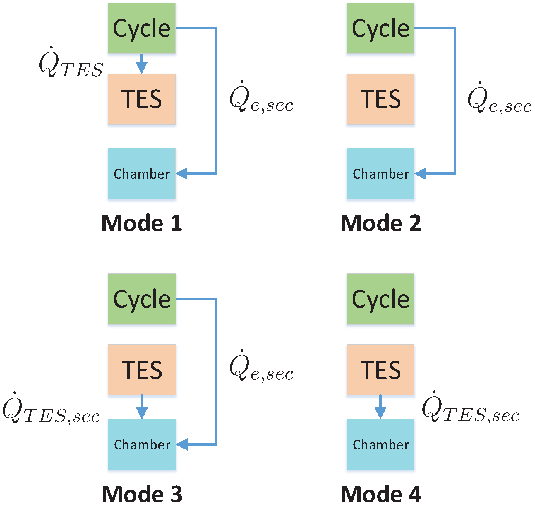
It must be remarked that, in the case of mode 2, the cooling demand is provided exclusively at the evaporator, and thus the TES tank is not involved and that is why the cooling power range does not depend on the freezing/melting boundary location. However, in mode 4, ${\dot{Q}}_{TES,sec}$ depends on the charge ratio, which decreases as the TES is discharged. Operating mode 3 is merely a combination of the previously described modes, where two independent secondary fluid circuits are used, and thus the cooling power ranges are the same as those presented for modes 2 and 4. Nevertheless, when operating in mode 1, ${\dot{Q}}_{e,sec}$ and ${\dot{Q}}_{TES}$ are strongly correlated, because the refrigerant circulates through the evaporator and the TES tank, then both flows merge at the compressor intake (point A in Figure 1). 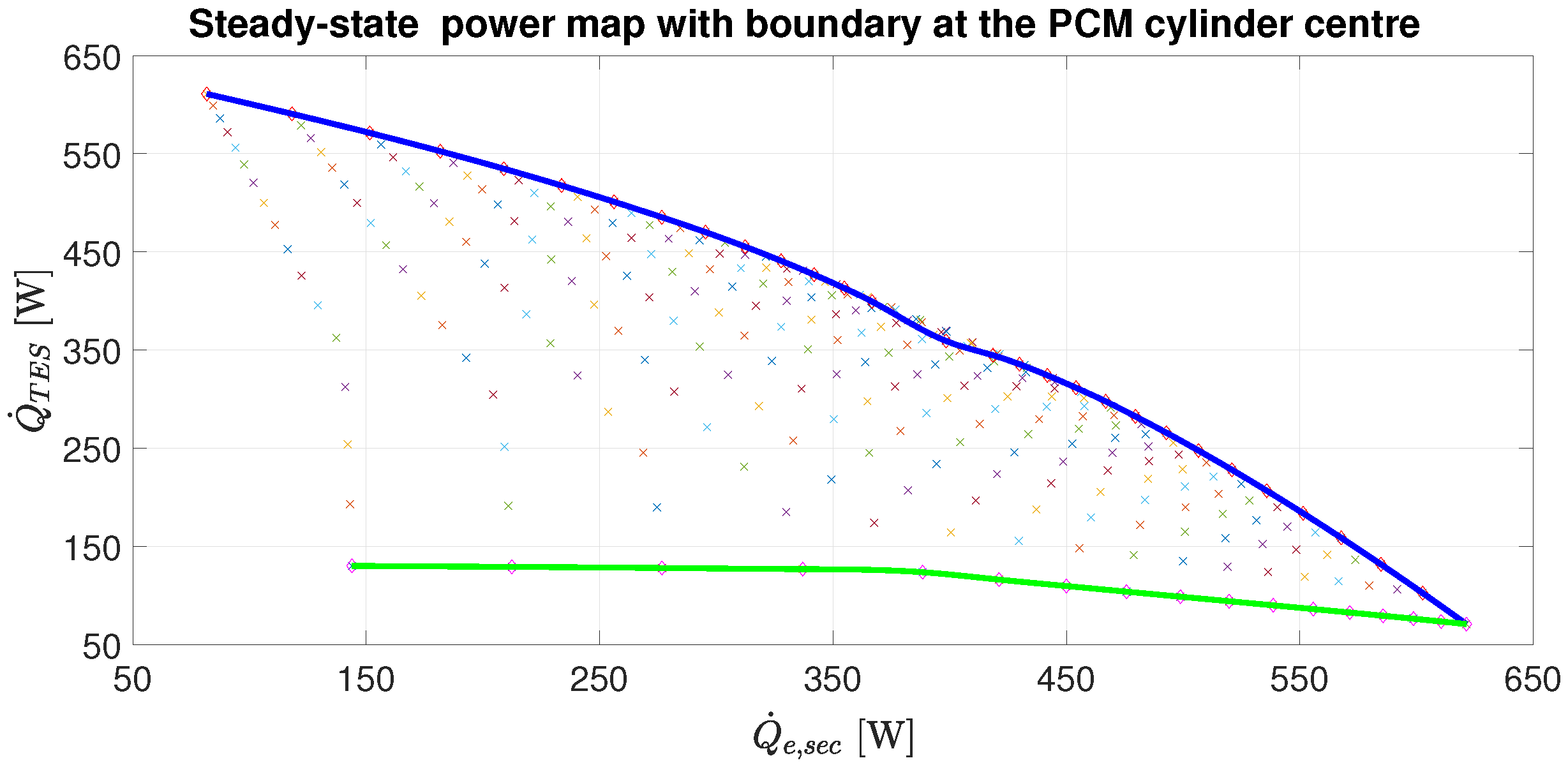Therefore, the ranges indicated in Table 4 are not completely rigorous, since they include some unachievable points. As an illustrative example, Figure 8 shows the steady-state map between ${\dot{Q}}_{e,sec}$ and ${\dot{Q}}_{TES}$ when the freezing boundary locates at the PCM cylinder centre, where the continuous lines represent the overall limits and the small crosses indicate a number of steady-state achievable points.

Similar plots have been obtained for different locations of the freezing boundary, which are not included here for the sake of brevity. Notice that the cooling demand ${\dot{Q}}_{sec}$ in operating mode 1 must be completely satisfied by ${\dot{Q}}_{e,sec}$, since ${\dot{Q}}_{TES,sec}$ is zero. Therefore, the maximum charging power ${\dot{Q}}_{TES}$ is shown to be constrained by the cooling demand.

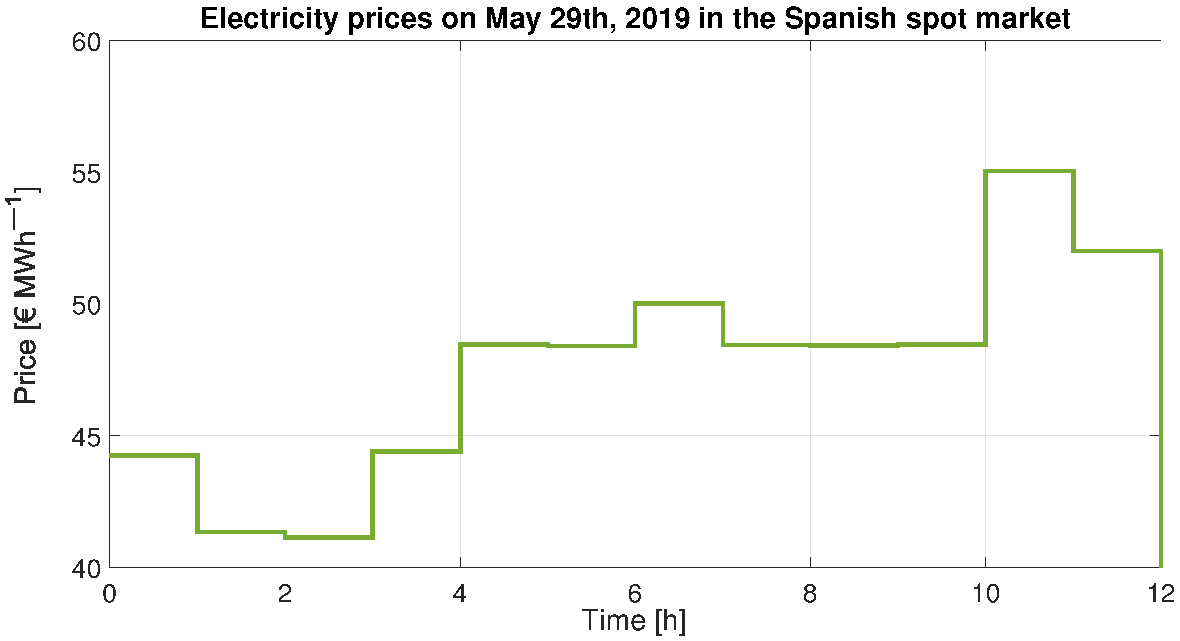
5.3. Energy Price

Realistic energy price evolution throughout the day is applied to the optimization problem. Figure 9 depicts the electricity prices corresponding to a given day (29 May 2019) in the Spanish spot market [31].

These prices, once scaled, are considered as the cost of the cooling power production at the evaporator, $w_{e,sec}$ in Equation (22), as well as the cost of the TES charging power, $w_{TES}$. However, $w_{TES,sec}$ is assumed to be zero, given that no extra cost is involved when using the previously produced cold energy, beyond the electric power devoted to pumping the secondary fluid, which is not considered in the objective function detailed in Equation (22).

5.4. Operating Mode Scheduling

If the demand profile shown in Figure 7 is analysed together with the cooling power constraints shown in Table 4 and the energy prices shown in Figure 9, it can be observed that, approximately, during the first 5 h, the cooling demand ${\dot{Q}}_{sec}$ can be satisfied by using only ${\dot{Q}}_{e,sec}$, given the power ranges for modes 1 and 2 presented in Table 4. It may be interesting to charge the TES tank during this period, taking advantage of the low energy price, but in any case the maximum charging power is constrained by the cooling demand, which must be satisfied in mode 1 by the refrigeration cycle. However, from $t=$ 5 h, the cooling demand ${\dot{Q}}_{sec}$ is too high to be satisfied only by ${\dot{Q}}_{e,sec}$, being necessary to turn to ${\dot{Q}}_{TES,sec}$ to complement the cooling power produced at the evaporator. Then, during the peak period until $t=$ 8 h, the TES tank is intended to be discharged, avoiding as much as possible the direct cooling power production due to the high price corresponding to this period. That is when the high charge ratio achieved previously comes handy. Finally, at the end of the day, the cooling demand is again low enough to allow modes 1 and 2 to be scheduled, thus the TES tank might be also charged during this off-peak period.

In the light of the previous analysis, a certain operating mode scheduling must be proposed to make use of the TES tank as a cold-energy storage unit, as efficiently as possible, according to economic criteria. This operating mode scheduling affects the optimization problem posed in Section 4.3 through the feasibility constraints described in (19), as schematically shown in Figure 10.

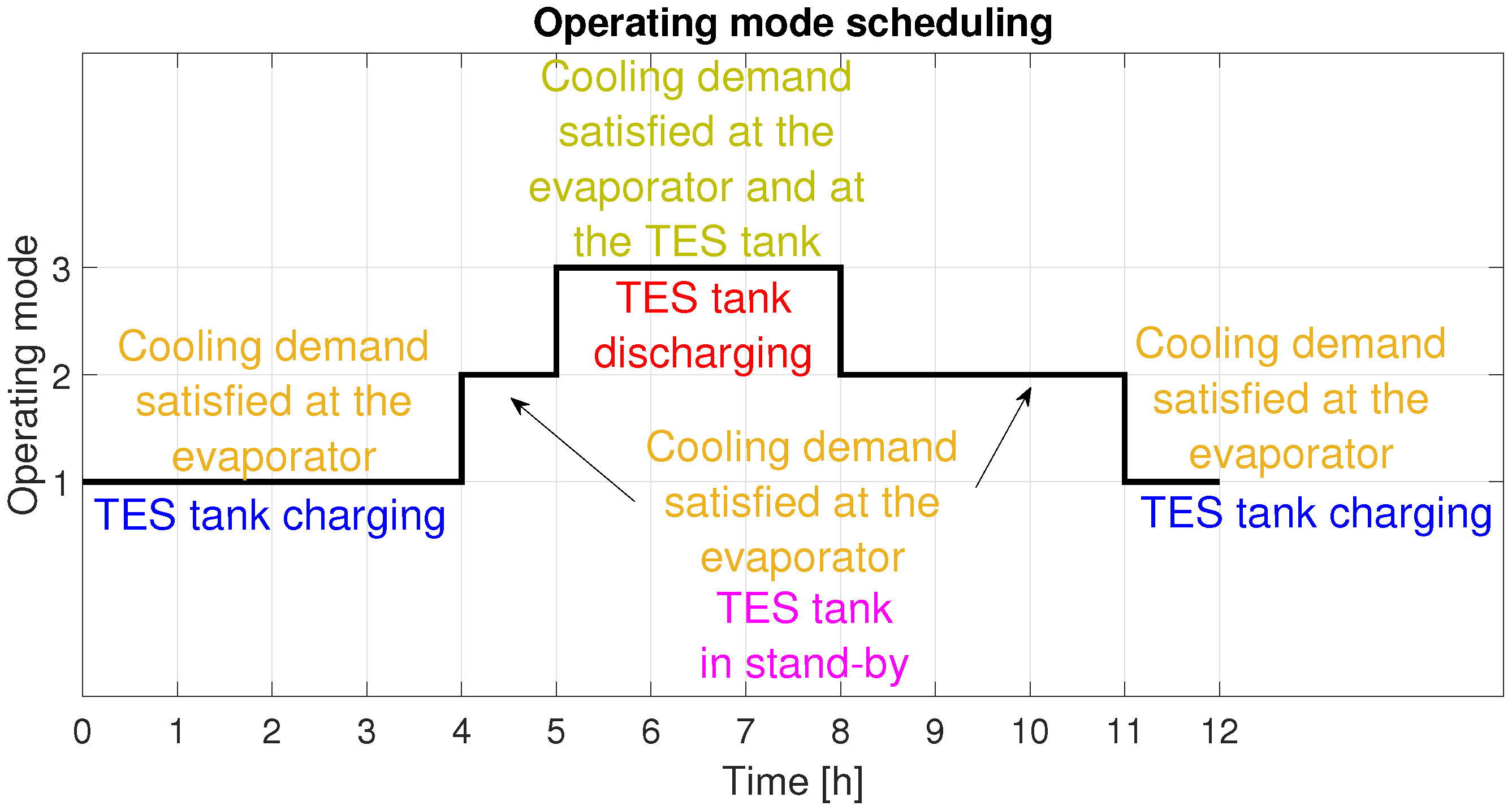
Figure 11 shows a proposed operating mode scheduling for the specific demand profile introduced in Figure 7, according to the power constraints analysed in Section 5.2 and the energy price profile shown in Figure 9.

As observed in Figure 11, the TES tank is scheduled to be charged during the off-peak periods at the beginning and at the end of the day, when the cost of cooling power production is lower. Given that the demand is low but not zero during these periods, operating mode 1 is scheduled, in such a way that the cooling demand is satisfied exclusively at the evaporator. Furthermore, the cold-energy stored in the TES tank is scheduled to be released during the peak period, complementing the cooling power provided to the secondary fluid at the evaporator to meet the cooling demand (operating mode 3). Two intermediate periods when the TES tank is not charged nor discharged, but in stand-by (operating mode 2), have been inserted between the charging and discharging periods, given that the cooling demand can be satisfied at the evaporator and it is certainly more interesting from an economic point of view to ensure the cooling demand satisfaction during all the peak period, when the contribution of the TES tank is imperative. Moreover, once the peak period is finished, it might be more interesting to concentrate the TES tank charging during the central hours of the off-peak period, when the economic cost of cooling power production is lowest.

5.5. Simulation Results

Some simulation results of the proposed scheduling strategy are presented in this subsection, where they are also compared to the performance of the original refrigeration system without energy storage, regarding both economic cost and constraint meeting.

Given the cooling demand shown in Figure 7 and the energy price profile shown in Figure 9, the references of the cooling powers are computed every hour. However, the dynamics related to heat transfer within the TES tank require an internal sampling time of the prediction model of 10 min. The latter could be reduced to increase accuracy, at the expense of greater computational load of the predictive scheduling strategy. Safety limits ${\gamma }_{TES}^{min}$ = 0.05 and ${\gamma }_{TES}^{max}$ = 0.95 have been considered, while a prediction horizon $PH$ = 4 is set. At the initial state of the TES tank, the intermediate fluid is assumed to be in thermal equilibrium with the PCM cylinders ($T_{int}(t=0)=T_{pcm}^{lat}$), whereas the initial enthalpy distribution of the latter is such that ${\gamma }_{TES}(t=0)$ = 0.35.

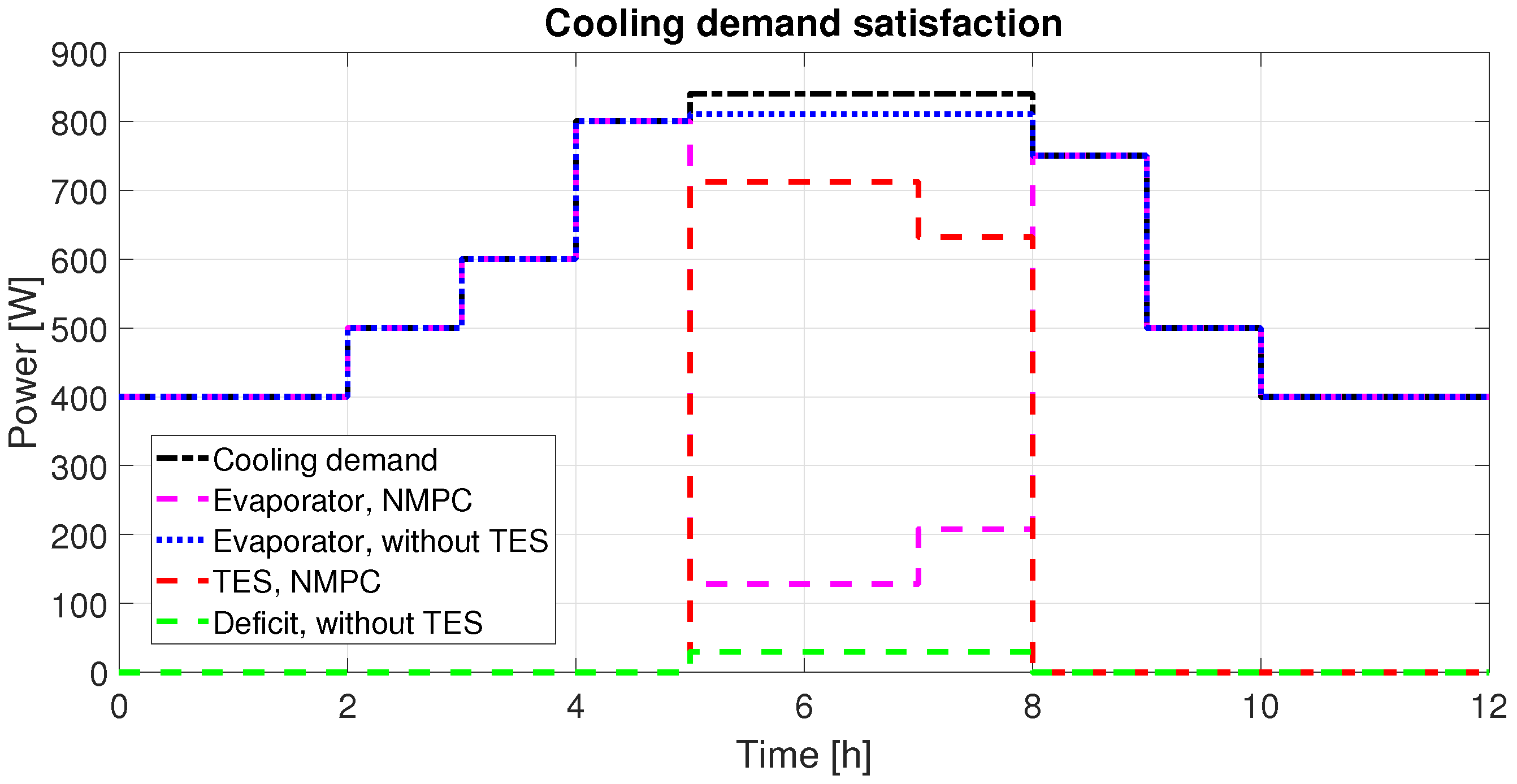
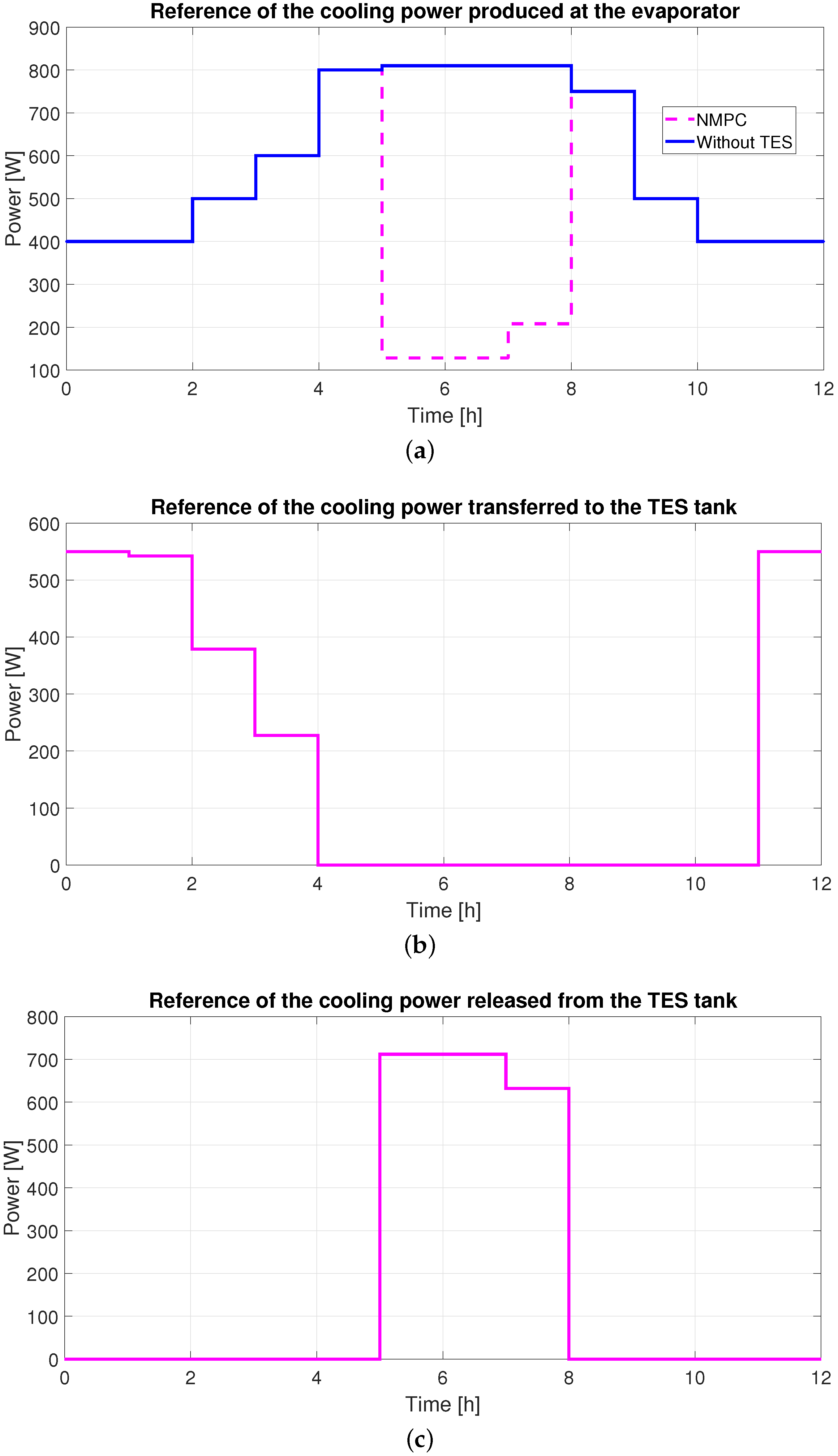
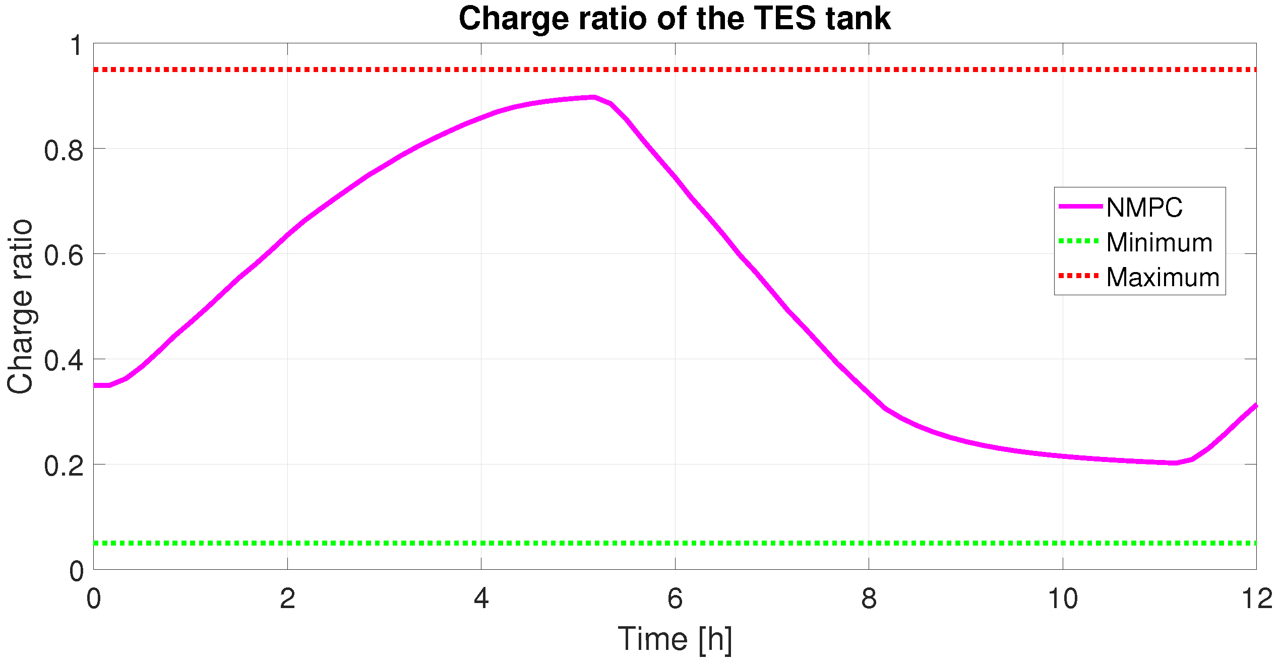
Figure 12 shows the performance of both the proposed scheduling strategy for the TES-backed-up system and the refrigeration cycle without TES, concerning the satisfaction of the cooling demand. Furthermore, Figure 13 shows the three references of the relevant cooling powers, whereas Figure 14 represents the charge ratio of the TES tank in the proposed scheduling strategy. Moreover, Figure 15 shows the temperature of the intermediate fluid, as well as the distribution of the temperature field of the PCM cylinders in the cooling, charging, and discharging processes.

Figure 12 shows that the refrigeration cycle without energy storage is not able to satisfy the cooling demand peak from t = 5 h to t = 8 h, thus incurring in some cooling power deficit, which is remarked in Figure 12. However, the TES-backed-up refrigeration cycle operated according to the proposed scheduling strategy is shown to provide the required cooling power to the secondary fluid by combining the power produced at the evaporator and the TES tank contribution during the peak period. To do this, the TES tank is charged during the off-peak periods, as shown in Figure 13b. The charge ratio is shown to be kept within the safety limits, as depicted in Figure 14, whereas a great deal of the energy capacity of the TES tank is used along the day. Notice in Figure 15a that, during the charging processes, the temperature of the intermediate fluid is below $T_{pcm}^{lat}$, being over $T_{pcm}^{lat}$ in the discharging process; in the stand-by processes, the thermal inertia of the intermediate fluid causes that, while approaching the thermal equilibrium with the PCM cylinders at $T_{pcm}^{lat}$, the latter continues charging/discharging while the residual cold energy is transferred. The distribution of temperatures within the PCM cylinders represented in Figure 15b show how the layers are quitting the latent zone from the outermost layer to the innermost, both in charging and discharging processes, as their latent energy depletes.

The performance of the low-level cooling power controller is not analysed in this work for the sake of brevity, since it is analysed in depth in [25], thus no plots of the actual control actions are included in this work. In any case, some important issues concerning this control layer will be remarked upon. The settling time of the cooling power closed loop turns out to be small enough to assume, given the scheduling time, that the required cooling powers are almost immediately provided, as long as the computed references are feasible, which is ensured by the power constraints met by the scheduler. The hypothesis about the separation between the time scales considered in the modelling stage is confirmed in the aforementioned work. Concerning the charging and discharging cooling powers, constant cold energy supply/release is achieved by increasing the mass flow of the refrigerant/secondary fluid as the thermal resistance caused by the cylindrical shell in sensible zone grows. Further details about the performance of the cooling power controller can be found in [25].

Regarding economic cost, the overall energy costs along the day of both the proposed scheduling strategy for the TES-backed-up cycle and the original system are gathered in

Table 5. Economic cost comparison of the proposed scheduling strategy for the TES-backed-up cycle and the original system without TES.

System	Economic Cost [Monetary Unit]	Reduction [%]
Refrigeration system without TES	20.82	–
TES-backed-up cycle	14.84	28.72

, as well as the achieved reduction. Notice that, in the case of the refrigeration cycle without storage, it is assumed that the energy deficit shown in Figure 12 must be bought at the market price detailed in Figure 9.

Obviously, the achieved reduction on the operating cost would come at a certain price in terms of CAPEX (capital expenditure). The economic analysis performed in this work is not intended to be comprehensive, but to throw some light on the high economic potential of such energy storage systems, which not only can ensure the satisfaction of demanding cooling load profiles, but they can also lead to significant cost reduction when properly operated. However, the simulation results highlight the need for suitable predictive scheduling strategies to manage the stored cold energy within the latent zone and fit the cooling power limits of a given facility. Indeed, the latter have been shown to vary significantly when the energy storage system is added to the original refrigeration cycle, both in charging and discharging processes.

5.6. Sensitivity Analysis

Some simulations of the proposed scheduling strategy considering parametric uncertainty are presented in this subsection. Given the design of the TES tank described in Section 2, minor uncertainty is expected to be devoted to geometry, constructive materials, working fluids, and their thermodynamic properties. Nevertheless, a simple heat transfer model is used to compute the cooling power transferred between the PCM cylinders and the intermediate fluid ${\dot{Q}}_{pcm}$, where a probably uncertain heat transfer coefficient computed by classical correlations for natural convection [32] has been considered to compute the thermal resistance $R_{pcm}^{conv,ext}$ in Equation (3). Moreover, the assumption of homogeneous heat transfer between the PCM cylinders and the intermediate fluid could lead to some degree of uncertainty regarding the cooling power calculation and then the evolution of the temperature of the intermediate fluid $T_{int}$. In order to assess the robustness of the proposed scheduling strategy against this kind of uncertainty, the latent temperature $T_{pcm}^{lat}$ considered by the prediction model will be artificially modified. The latter is usually precisely known by design, but if an uncertain value was considered in the prediction model, it would strongly affect the calculation of both TES charging and discharging cooling powers, which in turn determine how the intermediate fluid evolves. Therefore, the consideration of some uncertainty in the latent temperature $T_{pcm}^{lat}$ is just a simplified way of inducing uncertainty in all cooling power calculation within the TES tank.

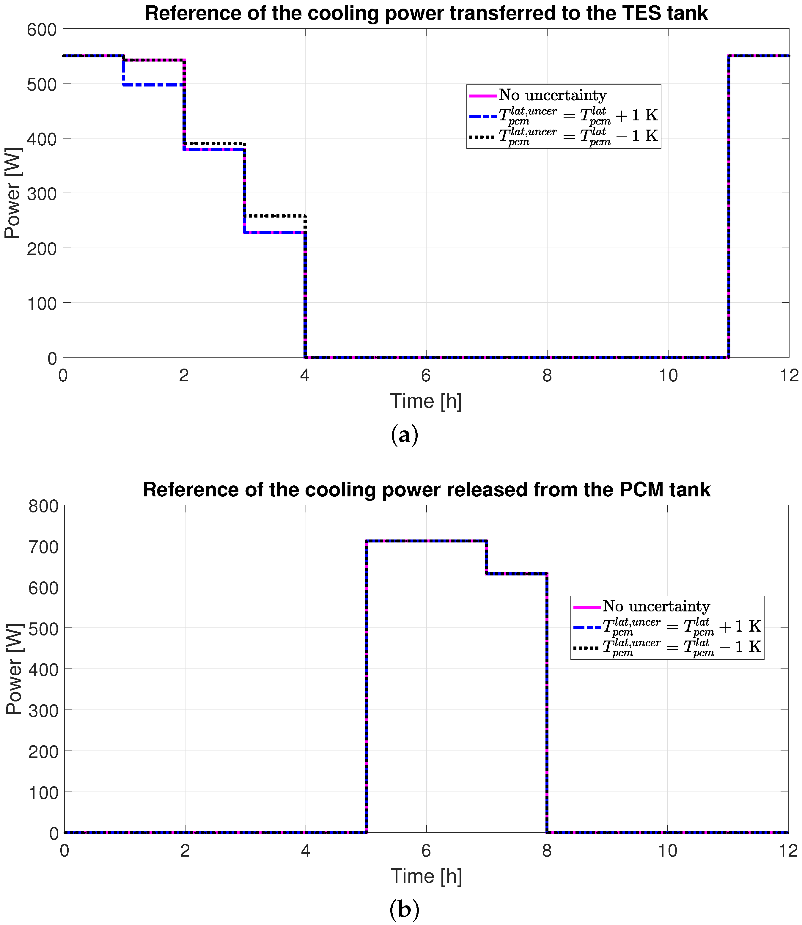
Figure 16 shows the references of the TES charging/discharging cooling powers ${\dot{Q}}_{TES}$ and ${\dot{Q}}_{TES,sec}$, when some uncertainty in $T_{pcm}^{lat}$ is considered. This temperature has been increased/decreased in 1 K from the nominal value in the prediction model. Given the variations of the intermediate temperature for the nominal case shown in Figure 15a, the considered increment/decrement is high enough to cause significant uncertainty in the prediction model with respect to the accurate model used for the plant simulation. Furthermore, Figure 17 compares the TES charge ratio for the three cases.

It is shown in Figure 17 that the proposed scheduling strategy provides very similar results for the references of the charging and discharging cooling powers, in spite of the significant uncertainty in the cooling power calculation and thus in the estimated charge ratio. In the case of ${\dot{Q}}_{TES,sec}$, the references are identical, as shown in Figure 16b, but some appreciable differences appear in Figure 16a regarding the charging power. The latter variations are due to the greater closeness to the upper limit imposed on the charge ratio in the case of the charging process, as represented in Figure 17. Therefore, the proposed scheduling strategy presents a suitable degree of robustness to significant modelling errors, ensuring cooling demand is satisfied and that the limits of the latent zone are met even if significant errors are introduced in the cooling power calculation.

6. Conclusions and Future Work

In this work, cold-energy management of a novel setup including a thermal energy storage tank based on phase change materials that complements a refrigeration facility has been addressed. The design of the upgrading process undertaken on the refrigeration facility to include the storage tank has been summarily described, along with the main features of the storage unit. Concerning the modelling, from a very detailed dynamic model previously developed, a simplified model focused on the slower dynamics related to heat transfer within the storage tank has been proposed to act as the prediction model in the scheduling optimization.

A layered scheduling and control strategy has been proposed, where a non-linear predictive scheduler computes the references of the main cooling powers involved, whereas the low-level controller ensures the achievement of the required cooling powers. The predictive scheduling problem is posed as a non-linear optimization with constraints due to cooling demand satisfaction, power feasibility, and latency limits, while considering economic criteria in the objective function.

A case study has been analysed, where a challenging load forecast that requires scheduling of different operating modes must be satisfied. The proposed strategy has been shown to ensure the cooling demand satisfaction and meeting of constraints while reducing the daily operating cost by up to 28% when compared to the refrigeration cycle without TES. Moreover, the latter fails in satisfying the cooling load during the entire day. A sensitivity analysis of the proposed strategy has shown it to provide satisfactory performance even when significant uncertainty in the prediction model is considered.

As future work, the application of the proposed strategy to the experimental plant is scheduled to be performed as soon as the upgrading process undertaken on the facility is finished. Furthermore, the development of an economic NMPC strategy is devised [33], as well as the stability analysis of the proposed NMPC-based scheduling strategy.

References

1. Raveendran, P.S.; Sekhar, S.J. Performance studies on a domestic refrigerators retrofitted with building-integrated water-cooled condenser. Energy Build. 2017, 134, 1–10. [Google Scholar] [CrossRef]
2. Ruz, M.L.; Garrido, J.; Vázquez, F.; Morilla, F. A hybrid modeling approach for steady-state optimal operation of vapor compression refrigeration cycles. Appl. Therm. Eng. 2017, 120, 74–87. [Google Scholar] [CrossRef]
3. Jain, N.; Alleyne, A.G. Exergy-based optimal control of a vapor compression system. Energy Convers. Manag. 2015, 92, 353–365. [Google Scholar] [CrossRef]
4. Espejel-Blanco, D.F.; Hoyo-Montaño, J.A.; Arau, J.; Valencia-Palomo, G.; García-Barrientos, A.; Hernández-De-León, H.R.; Camas-Anzueto, J.L. HVAC Control System Using Predicted Mean Vote Index for Energy Savings in Buildings. Buildings 2022, 12, 38. [Google Scholar] [CrossRef]
5. Kou, X.; Du, Y.; Li, F.; Pulgar-Painemal, H.; Zandi, H.; Dong, J.; Olama, M.M. Model-Based and Data-Driven HVAC Control Strategies for Residential Demand Response. IEEE Open Access J. Power Energy 2021, 8, 186–197. [Google Scholar] [CrossRef]
6. Macieira, P.; Gomes, L.; Vale, Z. Energy Management Model for HVAC Control Supported by Reinforcement Learning. Energies 2021, 14, 8210. [Google Scholar] [CrossRef]
7. Navas, S.J.; Rubio, F.R.; Ollero, P.; Lemos, J.M. Optimal control applied to distributed solar collector fields with partial radiation. Sol. Energy 2018, 159, 811–819. [Google Scholar] [CrossRef]
8. MacCracken, M.M. Thermal energy storage myths. Energy Eng. 2004, 101, 69–80. [Google Scholar] [CrossRef]
9. Rismanchi, B.; Saidur, R.; BoroumandJazi, G.; Ahmed, S. Energy, exergy and environmental analysis of cold thermal energy storage (CTES) systems. Renew. Sustain. Energy Rev. 2012, 16, 5741–5746. [Google Scholar] [CrossRef]
10. Oró, E.; De Gracia, A.; Castell, A.; Farid, M.; Cabeza, L. Review on phase change materials (PCMs) for cold thermal energy storage applications. Appl. Energy 2012, 99, 513–533. [Google Scholar] [CrossRef] [Green Version]
11. Mehling, H.; Cabeza, L.F. Heat and Cold Storage with PCM; Springer: Berlin/Heidelberg, Germany, 2008. [Google Scholar]
12. Bista, S.; Hosseini, S.E.; Owens, E.; Phillips, G. Performance improvement and energy consumption reduction in refrigeration systems using phase change material (PCM). Appl. Therm. Eng. 2018, 142, 723–735. [Google Scholar] [CrossRef]
13. Dutil, Y.; Rousse, D.R.; Salah, N.B.; Lassue, S.; Zalewski, L. A review on phase-change materials: Mathematical modeling and simulations. Renew. Sustain. Energy Rev. 2011, 15, 112–130. [Google Scholar] [CrossRef]
14. Berdja, M.; Hamid, A.; M’ahmed, C.; Sari, O. Novel approach to optimize the dimensions of phase change material thermal storage heat exchanger in refrigeration systems. Int. J. Energy Res. 2019, 43, 231–242. [Google Scholar] [CrossRef]
15. Wang, F.; Maidment, G.; Missenden, J.; Tozer, R. The novel use of phase change materials in refrigeration plant. Part 1: Experimental investigation. Appl. Therm. Eng. 2007, 27, 2893–2901. [Google Scholar] [CrossRef]
16. Wang, F.; Maidment, G.; Missenden, J.; Tozer, R. The novel use of phase change materials in refrigeration plant. Part 2: Dynamic simulation model for the combined system. Appl. Therm. Eng. 2007, 27, 2902–2910. [Google Scholar] [CrossRef]
17. Wang, F.; Maidment, G.; Missenden, J.; Tozer, R. The novel use of phase change materials in refrigeration plant. Part 3: PCM for control and energy savings. Appl. Therm. Eng. 2007, 27, 2911–2918. [Google Scholar] [CrossRef]
18. Mosaffa, A.; Farshi, L.G.; Ferreira, C.I.; Rosen, M. Advanced exergy analysis of an air conditioning system incorporating thermal energy storage. Energy 2014, 77, 945–952. [Google Scholar] [CrossRef]
19. Bejarano, G.; Ortega, M.G.; Normey-Rico, J.E.; Rubio, F.R. Optimal control analysis and Practical NMPC applied to refrigeration systems. ISA Trans. 2020, 107, 90–106. [Google Scholar] [CrossRef]
20. Yao, Y.; Shekhar, D.K. State of the art review on model predictive control (MPC) in Heating Ventilation and Air-conditioning (HVAC) field. Build. Environ. 2021, 200, 107952. [Google Scholar] [CrossRef]
21. Shafiei, S.E.; Stoustrup, J.; Rasmussen, H. Model predictive control for flexible power consumption of large-scale refrigeration systems. In Proceedings of the American Control Conference (ACC), Portland, OR, USA, 4–6 June 2014; pp. 412–417. [Google Scholar] [CrossRef] [Green Version]
22. Shafiei, S.E.; Alleyne, A. Model predictive control of hybrid thermal energy systems in transport refrigeration. Appl. Therm. Eng. 2015, 82, 264–280. [Google Scholar] [CrossRef]
23. Schalbart, P.; Leducq, D.; Alvarez, G. Ice-cream storage energy efficiency with model predictive control of a refrigeration system coupled to a PCM tank. Int. J. Refrig. 2015, 52, 140–150. [Google Scholar] [CrossRef]
24. Bejarano, G.; Suffo, J.J.; Vargas, M.; Ortega, M.G. Novel scheme for a PCM-based cold energy storage system. Design, modelling and simulation. Appl. Therm. Eng. 2018, 132, 256–274. [Google Scholar] [CrossRef]
25. Rodríguez, D.; Bejarano, G.; Vargas, M.; Lemos, J.M.; Ortega, M.G. Modelling and cooling power control of a TES-backed-up vapour-compression refrigeration system. Appl. Therm. Eng. 2020, 164, 114415. [Google Scholar] [CrossRef]
26. Bell, I.H.; Wronski, J.; Quoilin, S.; Lemort, V. Pure and Pseudo-pure Fluid Thermophysical Property Evaluation and the Open-Source Thermophysical Property Library CoolProp. Ind. Eng. Chem. Res. 2014, 53, 2498–2508. [Google Scholar] [CrossRef] [PubMed]
27. Alfaya, J.A.; Bejarano, G.; Ortega, M.G.; Rubio, F.R. Controllability analysis and robust control of a one-stage refrigeration system. Eur. J. Control 2015, 26, 53–62. [Google Scholar] [CrossRef]
28. Bejarano, G.; Rodríguez, D.; Alfaya, J.A.; Ortega, M.G.; Castaño, F. On identifying steady-state parameters of an experimental mechanical-compression refrigeration plant. Appl. Therm. Eng. 2016, 109, 318–333. [Google Scholar] [CrossRef]
29. Bejarano, G.; Vargas, M.; Ortega, M.G.; Castaño, F.; Normey-Rico, J.E. Efficient simulation strategy for PCM-based cold-energy storage systems. Appl. Therm. Eng. 2018, 139, 419–431. [Google Scholar] [CrossRef]
30. Bejarano, G.; Rodríguez, D.; Alfaya, J.A.; Gil, J.D.; Ortega, M.G. Optimization and Cascade Robust Temperature Control of a Refrigerated Chamber. In Proceedings of the 9th IFAC Symposium on Robust Control Design, Florianopolis, Brazil, 3–5 September 2018; pp. 110–115. [Google Scholar] [CrossRef]
31. REN—Redes Energéticas Nacionais, Lisbon (Portugal). Sistemas de Informação de Mercados de Energia. Available online: http://www.mercado.ren.pt/PT/Electr/ (accessed on 6 August 2020).
32. Bergman, T.L.; Incropera, F.P.; Lavine, A.S.; Dewitt, D.P. Fundamentals of Heat and Mass Transfer, 7th ed.; John Wiley & Sons: Hoboken, NJ, USA, 2011. [Google Scholar]
33. Ellis, M.; Durand, H.; Christofides, P.D. A tutorial review of economic model predictive control methods. J. Process Control 2014, 24, 1156–1178. [Google Scholar] [CrossRef]
Figure 1. Layout of the refrigeration system with cold-energy storage. (TES denotes thermal energy storage).
Mathematics 10 03167 g001
Figure 2. Layout of the TES-backed-up refrigeration plant under study.
Mathematics 10 03167 g002
Figure 3. Configuration of the thermal energy storage tank.
Mathematics 10 03167 g003
Figure 4. Simplified model of the TES-backed-up refrigeration system.
Mathematics 10 03167 g004
Figure 5. Most useful operating modes of the TES-backed-up refrigeration system.
Mathematics 10 03167 g005
Figure 6. Scheduling and control strategy for the TES-backed-up refrigeration system.
Mathematics 10 03167 g006
Figure 7. Cooling demand profile.
Mathematics 10 03167 g007
Figure 8. Steady-state cooling power map for mode 1 when the freezing/melting boundary locates at the PCM cylinder centre.
Mathematics 10 03167 g008
Figure 9. Electricity prices corresponding to 29 May 2019 in the Spanish spot market, once scaled into a 12 h timeframe [31].
Mathematics 10 03167 g009
Figure 10. Influence of the operating mode scheduling on the NMPC optimization problem.
Mathematics 10 03167 g010
Figure 11. Proposed operating mode scheduling.
Mathematics 10 03167 g011
Figure 12. Comparison of the cooling demand satisfaction between the proposed NMPC-based scheduling strategy and the refrigeration cycle without energy storage.
Mathematics 10 03167 g012
Figure 13. References on the relevant cooling powers for both the proposed scheduling strategy for the TES-backed-up system and the refrigeration cycle without energy storage. (a) Reference on Q ˙ e , s e c . (b) Reference on Q ˙ T E S . (c) Reference on Q ˙ T E S , s e c .
Mathematics 10 03167 g013
Figure 14. Charge ratio of the TES tank for the proposed scheduling strategy.
Mathematics 10 03167 g014
Figure 15. Temperature of the intermediate fluid and the cylindrical layers within the PCM cylinders. (a) Temperature of the TES tank intermediate fluid. (b) Distribution of temperature field within the PCM cylinders.
Mathematics 10 03167 g015
Figure 16. References of the TES charging/discharging cooling powers when some prediction model uncertainty is considered. (a) Reference on Q ˙ T E S . (b) Reference on Q ˙ T E S , s e c .
Mathematics 10 03167 g016
Figure 17. Charge ratio of the TES tank when some prediction model uncertainty is considered.
Mathematics 10 03167 g017