Coordination Control of Multi-Axis Steering and Active Suspension System for High-Mobility Emergency Rescue Vehicles

Abstract

This study proposes a coordinated control strategy to solve the coupling problem between the multi-axle steering system and the active suspension system of emergency rescue vehicles. Firstly, an eleven-degree-of-freedom coupling model of an emergency rescue vehicle is established. Secondly, a dual sliding mode (DSM) controller is designed for the multi-axle steering system and a dual linear quadratic regulator (DLQR) controller is designed for the active suspension system. Finally, the coordinated control strategy is designed, and the weight values are selected using the fuzzy algorithm. Results show that compared with the individual control, the root mean square (RMS) value of the body roll angle, roll angle acceleration, and yaw angle acceleration with coordinated control are reduced by 16.89%, 29.08%, and 27.75%, respectively. The proposed coordinated control strategy effectively improves the handling stability and ride comfort of the vehicle.

1. Introduction

Emergency rescue vehicles have a large load capacity and a high mass center, and the driving condition is complex. Furthermore, high mobility is required in rescue scenarios. A multi-axis steering system can reduce the turning diameter and improve vehicle mobility [1,2,3,4], and an active suspension system can adjust the output force of each suspension according to the road conditions and body status [5,6,7,8]. The two systems jointly determine the driving comfort and handling stability of the vehicle. When the vehicle is driving on uneven roads, the active suspension needs to be activated frequently and the vehicle needs to turn frequently to avoid obstacles, hence there is a complex coupling relationship between the steering and suspension systems [9,10]. 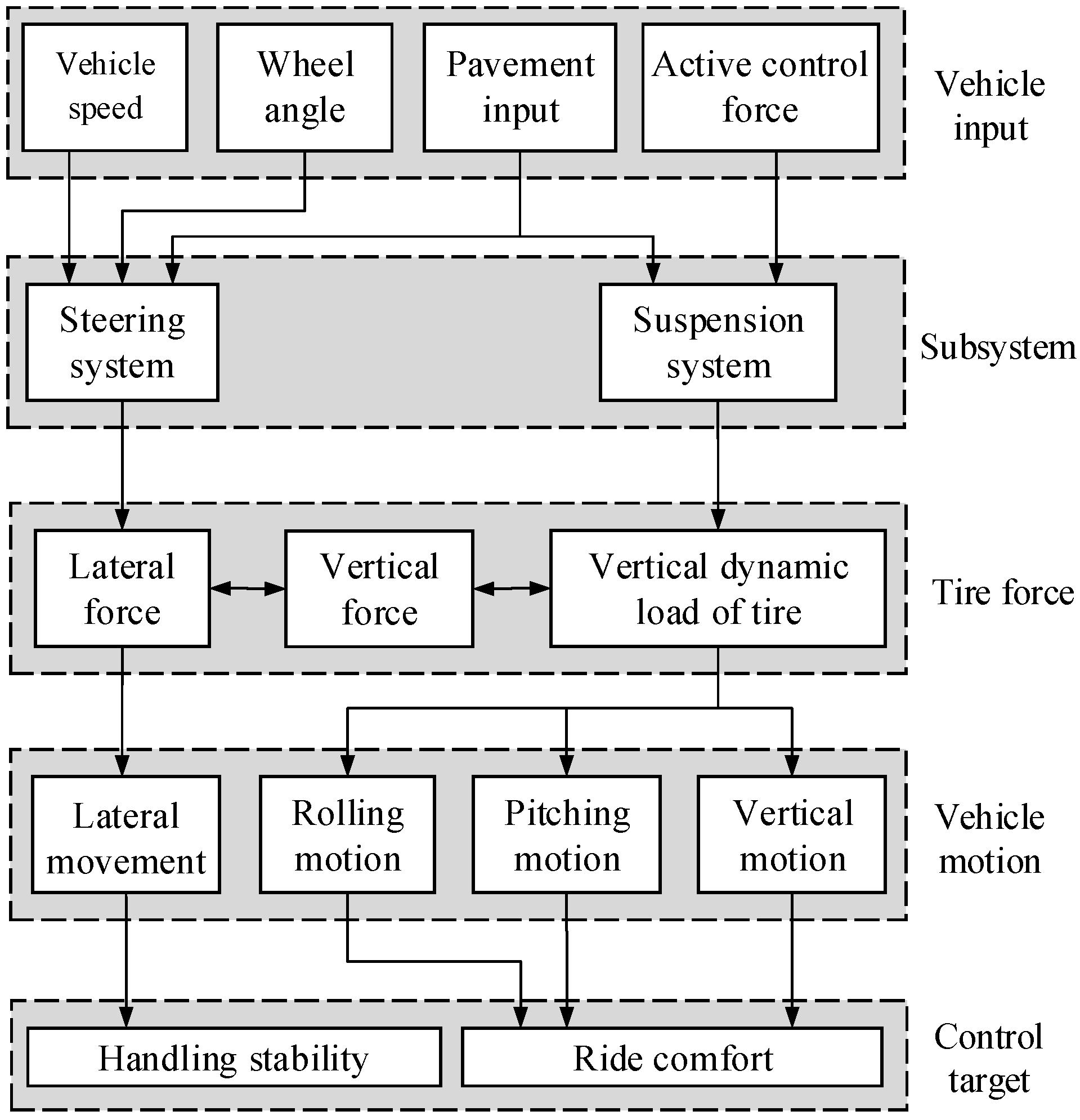The coupling mechanism of both systems is shown in Figure 1.

When the vehicle turns, the tire’s angle will change its lateral force, thus affecting the lateral movement and changing the handling stability of the vehicle. Meanwhile, the lateral movement of the vehicle makes the vertical load of the tire transfer laterally, affecting the driving comfort.

When the vehicle is driving on unstructured road, road excitation and active suspension control make the vertical dynamic load of the tires change, affecting the vertical, pitching, and rolling movements of the vehicle body, and further affecting the ride comfort. At the same time, the pitching and rolling movements of the body transfer the vertical load of the vehicle, changing the lateral force of the tires which further affects the lateral movement of the vehicle and the vehicle’s handling and stability [11,12,13,14]. The optimal effect cannot be achieved by controlling the two systems separately; hence, coordination control of the vehicle’s steering system and active suspension system is required [15,16,17,18,19].

The control strategies of active suspension mainly include optimal control [20], fuzzy control [21], neural network control [22], adaptive control [23], sliding mode control [24], etc. These studies do not take special consideration of steering conditions. The control strategies of multi-axle steering [5,6,7,8] take the side slip angle of mass center and yaw rate as the control target at the same time to ensure the handling stability of the vehicle in the steering process. These studies mostly design the linear controller based on the two-degree-of-freedom model and ignore a large number of nonlinear terms and external disturbances in the design process.

Many studies consider the coordination control of steering systems and active suspension systems. Harada et al. [25] designed the integrated controller based on the coupling model of the steering and suspension systems, and effectively improved the handling stability of the vehicle. Hac et al. [26] proposed a comprehensive closed-loop control strategy, which used integrated control to improve handling response and stability. Dahmain et al. [27] designed an integrated controller of all-wheel steering and active suspension systems to improve the mobility of the vehicle. Chokor et al. [28] designed an integrated controller for coordinating steering, yaw moment, and active suspension, which improved the overall performance of the vehicle. Yoshimura et al. [29,30] developed an integrated controller for the active suspension and steering systems using the fuzzy reasoning mechanism based on the linear dynamic model of the vehicle.

These studies mostly use two-axle vehicles as the research object, which simplifies the coupling effect between the steering and suspension systems. Compared with two-axle vehicles, the emergency rescue vehicle has a larger load capacity and a higher mass center, and its road condition is more complex. This makes the interaction between the steering system and the active suspension system more serious.

Taking the steering and suspension system of the high mobility emergency rescue vehicles as the research objective, this study establishes an eleven-degree-of-freedom coupling model and designs a dual sliding mode (DSM) controller and a dual linear quadratic regulator (DLQR) controller. Furthermore, a coordination control strategy is designed for the multi-axle steering system and the active suspension system. Finally, the effectiveness of the coordination control strategy is verified by experiments.

2. Coupling Dynamic Model of Steering and Suspension System

The eleven-degree-of-freedom (11-DOF) coupling model of the steering and suspension system is shown in Figure 2. The model includes the lateral motion along the y axis, the roll, pitch, and yaw motion of the sprung mass, the vertical motion of the center of mass, and the vertical motion of six unsprung masses.

A description of the model variables is given in

Table 1. Model variables (i = 1, 2,…, 6).

Variables	Meaning	Unit
m	Sprung mass	kg
Mwi	Each unsprung mass	kg
Zd	Vertical displacement of body mass center	m
zdi	Displacement at each suspension fulcrum	m
zwi	Each unsprung weight displacement	m
zri	Road surface input of each wheel	m
B	Wheel track	m
a	Distance between center of mass and front axle	m
b	Distance between center of mass and middle axle	m
c	Distance between center of mass and rear axle	m
θd	Body roll angle	rad
φd	Body pitch angle	rad
ωr	Body yaw angle	rad
αi	Included angle between axis direction and horizontal direction of each wheel	rad
β	Sideslip angle of centroid	rad
δi	Angle of each wheel	rad
Ix	Moment of inertia about x axis	kg·m2
Iy	Moment of inertia about y axis	kg·m2
Iz	Moment of inertia about z axis	kg·m2
ksi	Stiffness coefficient of each suspension spring	N/m
csi	Variable damping coefficient	N/(m·s)
kti	Stiffness coefficient of each tire	N/m
Ui	Actuation force of each active suspension	N
Fyi	Lateral force on each tire	N
u	Vehicle speed	m/s
hs	Distance from mass center of sprung mass to roll axis	m

.

According to Newton’s second law and Figure 1, we can derive the vehicle dynamics equations as follows:

$$mu(\dot{\beta }+{\omega }_r)-m_s{h}_s{\ddot{\theta }}_d={\displaystyle \sum _{i=1}^6{F}_{yi}\cos {\delta }_i},$$

(1)

$$I_z{\dot{\omega }}_r-I_{xz}{\ddot{\theta }}_d=a{F}_{y1}\cos {\delta }_1+a{F}_{y2}\cos {\delta }_2-b{F}_{y3}\cos {\delta }_3-b{F}_{y4}\cos {\delta }_4-c{F}_{y5}\cos {\delta }_5-c{F}_{y6}\cos {\delta }_6,$$

(2)

$$\begin{array}{ll}{I}_x{\ddot{\theta }}_d-m_s{h}_{s}u(\dot{\beta }+{\omega }_r)-I_{\mathit{xz}}{\dot{\omega }}_r& =\frac{B}{2}(-F_{s1}-F_{s3}-F_{s5}+F_{s2}+F_{s4}+F_{s6})+m_{s}g{h}_s{\theta }_d\\ & +\frac{B}{2}(U_1+U_3+U_5-U_2-U_4-U_6),\end{array}$$

(3)

$$m_s{\ddot{Z}}_d=-(F_{s1}+F_{s2}+F_{s3}+F_{s4}+F_{s5}+F_{s6})+U_1+U_2+U_3+U_4+U_5+U_6$$

(4)

$$I_y{\ddot{\phi }}_d-m_s{h}_{s}g{\phi }_d=a(F_{s1}+F_{s2}-U_1-U_2)-b(F_{s3}+F_{s4}-U_3-U_4)-c(F_{s5}+F_{s6}-U_5-U_6)$$

(5)

$$\begin{array}{l}{m}_{w1}{\ddot{z}}_{w1}=F_{s1}+U_1-F_{t1},\\ m_{w2}{\ddot{z}}_{w2}=F_{s2}+U_2-F_{t2},\\ m_{w3}{\ddot{z}}_{w3}=F_{s3}+U_3-F_{t3},\\ m_{w4}{\ddot{z}}_{w4}=F_{s4}+U_4-F_{t4},\\ m_{w5}{\ddot{z}}_{w5}=F_{s5}+U_5-F_{t5},\\ m_{w6}{\ddot{z}}_{w6}=F_{s6}+U_6-F_{t6},\end{array}$$

(6)

where, g is the gravity acceleration; F_si is the sum of spring force and damping force, $F_{si}=k_{si}(z_{di}-z_{wi})+c_{si}({\dot{z}}_{di}-{\dot{z}}_{wi})$, (i = 1,2,3,4,5,6); F_ti is the tire vertical force, $F_{\mathit{ti}}=k_{\mathit{ti}}(z_{\mathit{wi}}-z_{\mathit{ri}})$, (i = 1,2,3,4,5,6); F_yi is the lateral force on each tire,

$$F_{yi}=k_{\alpha i}{\alpha }_i,(i=1,2,3,4,5,6)$$

(7)

where, k_αi is the cornering stiffness of each tire.

The dynamic relationship between the six suspensions, the vehicle body connection points, the vertical motion of the vehicle body centroid, the pitch rotation, and the roll rotation can be expressed as:

$$\{\begin{array}{l}{z}_{d1}=Z_d-a\sin {\theta }_d-\frac{B}{2}\sin {\phi }_d;\\ z_{d2}=Z_d-a\sin {\theta }_d+\frac{B}{2}\sin {\phi }_d;\\ z_{d3}=Z_d+b\sin {\theta }_d-\frac{B}{2}\sin {\phi }_d;\\ z_{d4}=Z_d+b\sin {\theta }_d+\frac{B}{2}\sin {\phi }_d;\\ z_{d5}=Z_d+c\sin {\theta }_d-\frac{B}{2}\sin {\phi }_d;\\ z_{d6}=Z_d+c\sin {\theta }_d+\frac{B}{2}\sin {\phi }_d.\end{array}$$

(8)

The state variable X of the system is defined as:

$$X={\left[Z_d,{\theta }_d,{\phi }_d,z_{w1},\dots ,z_{w6},{\dot{Z}}_d,{\dot{\theta }}_d,{\dot{\phi }}_d,{\dot{z}}_{w1},\dots ,{\dot{z}}_{w6},\beta ,{\omega }_r\right]}^T$$

(9)

The external input of the system is:

$$W={\left[F_{s1},\dots ,F_{s6},F_{t1},\dots ,F_{t6},F_{y1},\dots ,F_{y6}\right]}^T$$

(10)

From Equations (1)–(6), it is evident that the nonlinearity of the coupling model is the tire force and suspension force. Therefore, the nonlinear force is taken as the external input of the vehicle state equation.

The control vector of the coupled system is defined as:

$$U={\left[U_1,U_2,U_3,U_4,U_5,U_6\right]}^T$$

(11)

The output vector of the coupled system is defined as:

$$Y={\left[Z_d,{\theta }_d,{\phi }_d,{\ddot{Z}}_d,{\ddot{\theta }}_d,{\ddot{\phi }}_d,z_{s1}-z_{w1},\dots ,z_{s6}-z_{w6},z_{w1}-z_{r1},\dots ,z_{w6}-z_{r6},\beta ,{\omega }_r\right]}^T$$

(12)

The state space expression of the coupling system is:

$$\{\begin{array}{l}\dot{X}=A_{1}X+B_{1}U+C_{1}W\\ Y=D_{1}X+E_{1}U+F_{1}W\end{array},$$

(13)

Where, $A_1=M^{-1}N,B_1=M^{-1}R,C_1=M^{-1}Q$, M, N, R and Q are coefficient matrices. They are shown in Appendix A.

3. DSM Controller of Multi-Axis Steering

A DSM controller was designed according to the yaw rate and the sideslip angle of the mass center. In addition, the output angle is decoupled in this section. Set the wheel angle at the front axle δ_f = δ₁ = δ₂, the wheel angle at the middle axle δ_m = δ₃ = δ₄, the wheel angle at the rear axle δ_r = δ₅ = δ₆, the tire cornering stiffness at the front axle k_f = k_α1 = k_α2, the tire cornering stiffness at the middle axle k_m = k_α3 = k_α4, and the tire cornering stiffness at the rear axle k_r = k_α5 = k_α6.

Equations (1) and (2) can then be expressed as:

$$mu(\dot{\beta }+{\omega }_r)=(k_f+k_m+k_r)\beta +\frac{1}{u}(a{k}_f-b{k}_m-c{k}_r){\omega }_r-k_f{\delta }_f-k_m{\delta }_m-k_r{\delta }_r+\Delta f_y,$$

(14)

$$I_z{\dot{\omega }}_r=(a{k}_f-b{k}_m-c{k}_r)\beta +\frac{1}{u}(a^2{k}_f+b^2{k}_m+c^2{k}_r){\omega }_r-a{k}_f{\delta }_f+b{k}_m{\delta }_m+c{k}_r{\delta }_r+\Delta m_z.$$

(15)

Set δ_m and δ_r as control quantities,

$$\{\begin{array}{l}{\delta }_{\beta }=-k_m{\delta }_m-k_r{\delta }_r\\ {\delta }_{\omega r}=b{k}_m{\delta }_m+c{k}_r{\delta }_r\end{array}.$$

(16)

According to Equations (14)–(16), we can obtain:

$$\dot{\beta }=\frac{k_f+k_m+k_r}{\mathit{mu}}\beta +(\frac{a{k}_f-b{k}_m-c{k}_r}{m{u}^2}-1){\omega }_r-\frac{k_f}{\mathit{mu}}{\delta }_f+\frac{1}{\mathit{mu}}{\delta }_{\beta }+\Delta F_y,$$

(17)

$${\dot{\omega }}_r=\frac{a{k}_f-b{k}_m-c{k}_r}{I_z}\beta +\frac{(a^2{k}_f+b^2{k}_m+c^2{k}_r)}{u{I}_z}{\omega }_r-\frac{a{k}_f}{I_z}{\delta }_f+\frac{1}{I_z}{\delta }_{\omega r}+\Delta M_z,$$

(18)

where, $\Delta F_y,\Delta M_z$ is the unmodeled term of the system, δ_β is the full-axis-angle output based on the side deflection angle of the mass center, and δ_ωr is the full-axis-angle output based on the yaw rate.

According to the integral sliding mode control [31], the sliding surface function based on the sideslip angle of the mass center can be designed as:

$$S_{\beta }=e_{\beta }+{\xi }_{\beta }{\int }_0^t{e}_{\beta }d\tau$$

(19)

The sliding surface function based on yaw rate can be designed as:

$$S_{\omega r}=e_{\omega r}+{\xi }_{\omega r}{\int }_0^t{e}_{\omega r}d\tau$$

(20)

where, $e_{\beta }=\beta -{\beta }_d$, $e_{\omega r}={\omega }_r-{\omega }_{rd}$, ${\beta }_d$ is the control target value of $\beta$, ${\omega }_{rd}$ is the control target value of ${\omega }_r$ and ξ_β and ξ_ωr are adjustable weight coefficients whose value is positive.

Taking the first-order derivative of Equations (19) and (20), we can obtain:

$$\begin{array}{ll}{\dot{S}}_{\beta }& ={\dot{e}}_{\beta }+{\xi }_{\beta }{e}_{\beta }\\ & =(\dot{\beta }-{\dot{\beta }}_d)+{\xi }_{\beta }(\beta -{\beta }_d)\\ & =(\frac{k_f+k_m+k_r}{mu}+{\xi }_{\beta })\beta +(\frac{a{k}_f-b{k}_m-c{k}_r}{m{u}^2}-1){\omega }_r-\frac{k_f}{mu}{\delta }_f+\frac{1}{mu}{\delta }_{\beta }-{\dot{\beta }}_d-{\xi }_{\beta }{\beta }_d,\end{array}$$

(21)

$$\begin{array}{ll}{\dot{S}}_{\omega r}& ={\dot{e}}_{\omega r}+\xi e_{\omega r}\\ & =({\dot{\omega }}_r-{\dot{\omega }}_{rd})+\xi ({\omega }_r-{\omega }_{rd})\\ & =\frac{a{k}_f-b{k}_m-c{k}_r}{I_z}\beta +(\frac{a^2{k}_f+b^2{k}_m+c^2{k}_r}{I_{z}u}+\xi ){\omega }_r-\frac{a{k}_f}{I_z}{\delta }_f+\frac{1}{I_z}{\delta }_{\omega r}-{\dot{\omega }}_{rd}-\xi {\omega }_{rd}.\end{array}$$

(22)

The reaching laws are:

$${\dot{S}}_{\beta }=-K_{\beta }{S}_{\beta }-{\epsilon }_{\beta }sgn(S_{\beta })$$

(23)

$${\dot{S}}_{\omega r}=-K_{\omega r}{S}_{\omega r}-{\epsilon }_{\omega r}sgn(S_{\omega r})$$

(24)

where, ${\epsilon }_{\beta },K_{\beta },K_{\omega r},{\epsilon }_{\omega r}$ are the undetermined coefficients, which can be obtained through a simulation trial.

According to Equations (19)–(24), the control laws can be obtained as:

$${\delta }_{\beta }=mu\left[\begin{array}{l}-(\frac{k_f+k_m+k_r}{mu}+{\xi }_{\beta })\beta -(\frac{a{k}_f-b{k}_m-c{k}_r}{m{u}^2}-1){\omega }_r\\ +\frac{k_f}{mu}{\delta }_f+{\xi }_{\beta }{\beta }_d+{\dot{\beta }}_d-K_{\beta }{S}_{\beta }-{\epsilon }_{\beta }sgn(S_{\beta })\end{array}\right]$$

(25)

$${\delta }_{\omega r}=I_z\left[\begin{array}{l}-(\frac{a{k}_f-b{k}_m-c{k}_r}{I_z})\beta -(\frac{a^2{k}_f+b^2{k}_m+c^2{k}_r}{I_{z}u}+\xi ){\omega }_r\\ +\frac{a{k}_f}{I_z}{\delta }_f+{\dot{\omega }}_{rd}+\xi {\omega }_{rd}-K_{\omega r}{S}_{\omega r}-{\epsilon }_{\omega r}sgn(S_{\omega r})\end{array}\right]$$

(26)

The Lyapunov functions of the sliding mode controller based on the sideslip angle of the mass center and the yaw rate are defined as:

$$V_{\beta }=\frac{1}{2}{S}_{\beta }^2$$

(27)

$$V_{\omega r}=\frac{1}{2}{S}_{\omega r}^2$$

(28)

After substituting Equation (25) into Equation (21), and Equation (26) into Equation (22), respectively, and calculating the first derivative of Lyapunov function shown in Equations (27) and (28), we can obtain:

$${\dot{V}}_{\beta }=S_{\beta }{\dot{S}}_{\beta }=-K_{\beta }{S}_{\beta }^2-S_{\beta }sgn(S_{\beta })\le 0$$

(29)

$${\dot{V}}_{\omega r}=S_{\omega r}{\dot{S}}_{\omega r}=-K_{\omega r}{S}_{\omega r}^2-S_{\omega r}sgn(S_{\omega r})\le 0$$

(30)

According to Equations (29) and (30), the first derivatives ${\dot{V}}_{\beta }$ and ${\dot{V}}_{\omega r}$ of the Lyapunov function are always less than zero, that is, given any initial value of $S_{\beta }(0)$ and $S_{\omega r}(0)$, $t\to \infty ,S_{\beta }(t)\to 0,S_{\omega r}(t)\to 0$. Therefore, the sliding mode controllers, based on the side slip angle of mass center and yaw rate, are stable.

Decoupling the δ_β and δ_ωr according to Equation (16), the wheel angles of the middle axle and the rear axle output by the controller can be obtained, as shown in Equation (31):

$$\{\begin{array}{l}{\delta }_m=-\frac{1}{c{k}_m-b{k}_m}{\delta }_{\omega r}-\frac{c}{c{k}_m-b{k}_m}{\delta }_{\beta }\\ {\delta }_r=\frac{1}{c{k}_r-b{k}_r}{\delta }_{\omega r}+\frac{b}{c{k}_r-b{k}_r}{\delta }_{\beta }\end{array}$$

(31)

4. DLQR Controller of Active Suspension

A DLQR controller includes an LQR integrated controller and an LQR roll controller. The LQR integrated controller is designed for the active suspension system to reduce the vertical acceleration, pitch angle, and roll angle of the vehicle. Furthermore, the LQR roll controller is designed to further control the roll angle during steering.

The output matrix Y₁ of the LQR integrated controller and the output matrix Y₂ of the LQR roll controller are expressed as:

$$Y_1=\left[{\ddot{Z}}_d,{\ddot{\theta }}_d,{\ddot{\phi }}_d,z_{d1}-z_{w1},\dots ,z_{d6}-z_{w6},z_{w1}-z_{r1},\dots ,z_{w6}-z_{r6}\right]$$

(32)

$$Y_2=\left[{\phi }_d,{\ddot{\phi }}_d,z_{d1}-z_{w1},\dots ,z_{d6}-z_{w6},z_{w1}-z_{r1},\dots ,z_{w6}-z_{r6}\right]$$

(33)

The output equations are:

$$Y_1=D_{1}X+E_1{U}_z+F_{1}W$$

(34)

$$Y_2=D_{2}X+E_2{U}_{\phi }+F_{2}W$$

(35)

where, D₁, E₁, F₁, D₂, E₂, and F₂ are coefficient matrices of the performance output equation, X is the state variable as shown in Equation (9) and W is the external input of the system as shown in Equation (10).

According to the LQR control [32], the objective function J₁ of the LQR integrated controller and the objective function J₂ of the LQR roll controller are:

$$\begin{array}{ll}{J}_1& ={\int }_0^{\infty }[q_1{\ddot{Z}}_d^2+q_2{\ddot{\theta }}_d^2+q_3{\ddot{\phi }}_d^2+q_4{(z_{d1}-z_{w1})}^2+q_5{(z_{d2}-z_{w2})}^2+q_6{(z_{d3}-z_{w3})}^2\\ & +q_7{(z_{d4}-z_{w4})}^2+q_8{(z_{d5}-z_{w5})}^2+q_9{(z_{d6}-z_{w6})}^2+q_{10}{(z_{w1}-z_{r1})}^2\\ & +q_{11}{(z_{w2}-z_{r2})}^2+q_{12}{(z_{w3}-z_{r3})}^2+q_{13}{(z_{w4}-z_{r4})}^2+q_{14}{(z_{w5}-z_{r5})}^2\\ & +q_{15}{(z_{w6}-z_{r6})}^2+q_{16}{U}_1^2+q_{17}{U}_2^2+q_{18}{U}_3^2+q_{19}{U}_4^2+q_{20}{U}_5^2+q_{21}{U}_6^2]dt\\ & ={\int }_0^{\infty }(Y_1^T{Q}_0{Y}_1+U_z^T{R}_0{U}_z)dt,\end{array}$$

(36)

$$\begin{array}{ll}{J}_2& ={\int }_0^{\infty }[s_1{\phi }_d^2+s_2{\ddot{\phi }}_d^2+s_3{(z_{d1}-z_{w1})}^2+s_4{(z_{d2}-z_{w2})}^2+s_5{(z_{d3}-z_{w3})}^2\\ & +s_6{(z_{d4}-z_{w4})}^2+s_7{(z_{d5}-z_{w5})}^2+s_8{(z_{d6}-z_{w6})}^2+s_9{(z_{w1}-z_{r1})}^2\\ & +s_{10}{(z_{w2}-z_{r2})}^2+s_{11}{(z_{w3}-z_{r3})}^2+s_{12}{(z_{w4}-z_{r4})}^2+s_{13}{(z_{w5}-z_{r5})}^2\\ & +s_{14}{(z_{w6}-z_{r6})}^2+s_{15}{U}_1^2+s_{16}{U}_2^2+s_{17}{U}_3^2+s_{18}{U}_4^2+s_{19}{U}_5^2+s_{20}{U}_6^2]dt\\ & ={\int }_0^{\infty }(Y_2^T{S}_0{Y}_2+U_{\phi }^T{T}_0{U}_{\phi })dt,\end{array}$$

(37)

where, $Q_0=diag(q_1{q}_2{q}_3\cdots q_{13}{q}_{14}{q}_{15})$ and $S_0=diag(s_1{s}_2{s}_3\cdots s_{13}{s}_{14}{s}_{15})$ are the weight coefficients of the Y₁ and Y₂, $R_0=diag(q_{16}{q}_{17}{q}_{18}{q}_{19}{q}_{20}{q}_{21})$ and $T_0=diag(s_{16}{s}_{17}{s}_{18}{s}_{19}{s}_{20}{s}_{21})$ are the weight coefficients of the U_z and U_φ.

By substituting Equation (34) into Equation (36), and Equation (35) into Equation (37), we can obtain:

$$J_1={\int }_0^{\infty }(X^T{Q}_{d}X+2D_1^T{N}_d{E}_1+U_z^T{R}_d{U}_z)dt$$

(38)

$$J_2={\int }_0^{\infty }(X^T{S}_{\phi }X+2D_2^T{N}_{\phi }{E}_2+U_{\phi }^T{R}_{\phi }{U}_{\phi })dt$$

(39)

where, $Q_d=D_1^T{Q}_0{D}_1$, $N_d=D_1^T{Q}_0{E}_1$, $R_d=E_1^T{Q}_0{E}_1+R_0$,$S_{\phi }=D_2^T{S}_0{D}_2$, $N_{\phi }=D_2^T{S}_0{E}_2$, $R_{\phi }=D_2^T{S}_0{E}_2+T_0$.

According to the optimal control theory, if the suspension actuation force U_zi = −K_zX and K_φi = −K_φX, then the objective function Equation (40) of the system can be minimized under the constraint conditions. Where K_z and K_φ are the optimal feedback gain matrices, $K_z=R_d^{-1}{N}_d^T+R_d^{-1}{B}_1^T{P}_1$, $K_{\phi }=R_{\phi }^{-1}{N}_{\phi }^T+R_{\phi }^{-1}{B}_2^T{P}_2$, and the matrixes P₁ and P₂ are obtained from the Riccati equation.

5. Coordinated Control of Multi-Axis Steering and Active Suspension Systems

5.1. Coordinated Control Strategy

The suspension system and steering system are two important coupling subsystems on the vehicle chassis, which jointly determine the ride comfort and handling stability of the vehicle. The coordinated control strategy of the multi-axis steering and active suspension systems is shown in Figure 3.

Evidently, the coordination control strategy designed in this paper includes the executive, control, and coordination layers. The executive layer consists of the multi-axis steering system and active suspension system, the control layer consists of both steering DSM and active suspension DLQR controllers, and the control layer consists of the upper coordination controller.

The upper coordination controller adjusts the weight coefficients K₁, K₂, and K₃ in real time according to the vehicle speed u and front wheel angle |δ_f|. To achieve the coordination of each sub-controller, the control rules are as follows:

$$\mathrm{I}\mathrm{f}\left(u>0and\left|{\delta }_f\right|<{\delta }_0\right),\mathrm{then}{K}_3=0.$$

Herein, the active suspension DLQR controller works to improve the smoothness of the vehicle. Relying solely on the integrated controller of the active suspension system can achieve satisfactory results; that is, the weight coefficient K₁ should be increased while the weight coefficient K₂ should be reduced. The multi-axis steering controller does not work, that is, K₃ = 0.

$$\mathrm{I}\mathrm{f}\left(u>0and\left|{\delta }_f\right|\ge {\delta }_0\right), \mathrm{then}{K}_3=1.$$

At this time, the vehicle is affected by lateral torque. The vehicle’s body will have a large roll angle, and the roll angle will increase with the increase in |δ_f|. Here, the main task is to improve the handling stability of the vehicle and reduce the body roll angle. The active suspension DLQR controller and the steering DSM controller work at the same time to reduce the weight coefficient K₁ and increase the weight coefficient K₂, where K₃ = 1.

Due to the real-time change of vehicle motion state, there are high requirements for the real-time performance of the weight coefficient, and it is impossible to establish an accurate mathematical relationship between the observation and the weight coefficient. Therefore, the weight coefficients K₁ and K₂ are obtained through fuzzy reasoning.

Considering the actual situation of emergency rescue in the field, the maximum of the |δ_f| is set to 32°, and the maximum speed is set to 40 km/h. Therefore, the input of the upper-level coordination controller is the front wheel angle |δ_f|∈[0, 32] and the vehicle speed u∈[0, 40]. The fuzzy subsets are {ZO, PS, PM, PB, PVB}, adopting the Gaussian membership function as shown in Figure 4.

The outputs are K₁∈[0, 1] and K₂∈[0, 1], and the fuzzy subsets are {PES, PVS, PS, PM, PB, PVB, PEB}, adopting the Gaussian membership function as shown in Figure 5. The fuzzy control rules of K₁ and K₂ are shown in

Table 2. The fuzzy control rules of K₁.

		δ1	ZO	PS	PM	PB	PVB
	K1
u
ZO			PES	PES	PVS	PS	PM
PS			PES	PVS	PS	PM	PB
PM			PVS	PM	PB	PB	PVB
PB			PS	PM	PB	PVB	PVB
PVB			PS	PB	PVB	PEB	PEB

and

Table 3. The fuzzy control rules of K₂.

Weight Coefficients	Fuzzy Control Rules
K1	PES	PVS	PS	PM	PB	PVB	PEB
K2	PEB	PEB	PB	PM	PS	PVS	PES

.

The actuation force U_i of the active suspension system is:

$$U_i=K_1{U}_{zi}+K_2{U}_{\phi i},i=1,2,\dots ,6.$$

(40)

5.2. Simulation Analysis

Taking the nonlinear coupling model as the control object, the MATLAB/Simulink simulation results of individual and coordination control are compared under two typical conditions. During individual control, the multi-axis steering system and the active suspension system are controlled independently. In the case of coordination control, the upper-level coordinated controller is used to control the two subsystems.

5.2.1. Step Angle

The vehicle ran on a class C pavement at 35 km/h, and the front axle angle was a step signal with an amplitude of π/6. The comparative simulation result of individual control and coordination control is shown in Figure 6, and the root mean square (RMS) values of performance indexes are shown in

Table 4. RMS values of the performance indexes under step steering.

Performance Index	Individual Control	Coordination Control
Roll angle (rad)	0.0607	0.0425 (↓ 29.98%)
Roll angle acceleration (rad/s2)	0.1635	0.1163 (↓ 28.87%)
Yaw angle acceleration (rad/s2)	0.0756	0.0581 (↓ 23.15%)
Lateral acceleration (m/s2)	3.1512	3.0642

.

As shown in Figure 6 and Table 4, compared with the individual control, the RMS value of roll angle was reduced by 29.98%, showing that the coordination controller can effectively reduce the roll angle generated by the vehicle when turning. Furthermore, the lateral acceleration has little difference, indicating that steering ability under coordination control is not weakened. The roll angle acceleration and yaw angle acceleration also decreased by 28.87% and 23.15%, respectively. Therefore, the proposed coordinated control can effectively improve the steering performance of the emergency rescue vehicle.

5.2.2. Double Lane Change

The vehicle then ran on a B-grade road surface at 35 km/h, and a double lane change was adopted. The comparative simulation result of individual control and coordination control is shown in Figure 7, and the RMS values of performance indexes are shown in

Table 5. RMS values of performance indexes under double line change conditions.

Performance Indexes	Individual Control	Coordination Control
Sideslip angle of centroid (rad)	0.0012	0.001 (↓ 16.67%)
Roll angle (rad)	0.0077	0.0056 (↓ 27.82%)
Roll angle velocity (rad/s)	0.0895	0.0626 (↓ 30.01%)
Roll angle acceleration (rad/s2)	0.2713	0.2134 (↓ 21.31%)

.

It can be seen from Figure 7 and Table 5 that under double line change conditions, compared with individual control, the RMS values of the sideslip angle of the centroid, the roll angle, roll angle velocity, and roll angle acceleration under the coordinated control were reduced by 16.67%, 27.82%, 30.01%, and 21.31%, respectively. In addition, the peak value of yaw angle speed was reduced, and the lateral acceleration was more stable, thus improving the vehicle’s turning ability. Ultimately, under the conditions of double line change, coordination control can effectively improve the stability and steering performance of the emergency rescue vehicle.

6. Experiment

The emergency rescue vehicle used in this paper is shown in Figure 8. The hydraulic cylinders are controlled by the electro-hydraulic servo valves and the pipelines connected with the two chambers of the hydraulic cylinders are equipped with pressure sensors. The steering hydraulic cylinders are controlled by proportional valves. The vehicle attitude, the accelerations of three coordinate axes, and the angular velocities of three coordinate axes are collected by the inertial measurement unit. The vehicle speed and wheel angle can be read out by the vehicle CAN bus. The main parameters of the heavy rescue vehicle are also shown in

Table 6. Main parameters of emergency rescue vehicles.

Parameters	Value of parameter
Weight (kg)	36,000
Number of wheels	6
Number of axles	3
Wheelbase of the first and second axle (m)	2.95
Wheelbase of the second and third axle (m)	1.65
Wheel track (m)	2.55
System pressure (Pa)	26 × 106
Rated flow of servo valve (L/min)	120

.

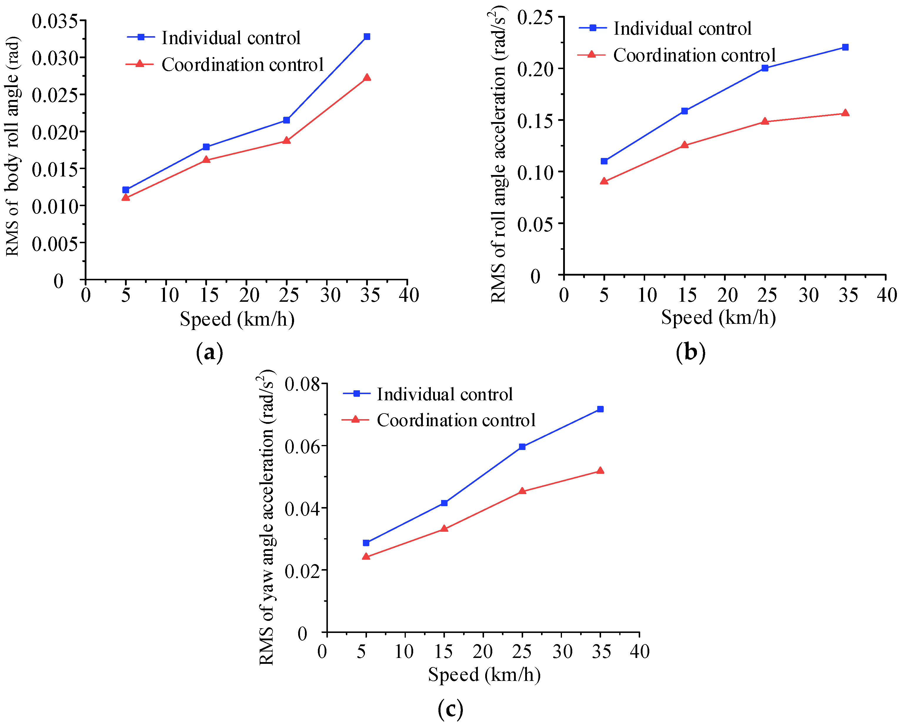
The vehicle ran on a class C pavement at 35 km/h, and the front axle angle was a step signal with amplitude of π/6. The coordinated control strategy proposed in this paper was used to control the whole vehicle and was compared with individual control to verify its effectiveness. Figure 9 shows a comparison diagram of the body roll angle, roll angle acceleration, and yaw angle acceleration at RMS value vehicle speeds of approximately 5 km/h, 15 km/h, 25 km/h, and 35 km/h.

It is evident therein that when the RMS value of vehicle speed reaches the abovementioned speeds, the body roll angle, roll angle acceleration, and yaw angle acceleration under coordinated control are reduced compared with those under individual control. In addition, the higher the speed, the more they reduce. This shows that coordinated control can effectively improve the handling stability of the vehicle. The test results showing the RMS value when the vehicle speed reaches 35 km/h are given in Figure 10. The RMS values of the performance indexes are calculated in

Table 7. RMS value of the performance index.

Performance Index	Individual Control	Coordination Control
Roll angle (rad)	0.0412	0.0325 (↓ 21.12%)
Roll angle acceleration (rad/s2)	0.2204	0.1563 (↓ 29.08%)
Yaw angular acceleration (rad/s2)	0.0717	0.0518 (↓ 27.75%)
Vehicle speed (km/h)	34.8869	34.7564
Lateral acceleration (m/s2)	1.5262	1.4985

.

It can be seen from Figure 10a,b that the roll angle and lateral acceleration change significantly when t = 5 s, indicating that the vehicle turns left when t = 5 s. Before the vehicle turns (t < 5 s), the control effects of the two control methods are close. After the vehicle turns (t ≥ 5 s), the roll angle under coordination control is obviously smaller than that under individual control, and the lateral acceleration is more stable. When the vehicle is turning, the coordination controller can adjust the weight coefficients K₁, K₂, and K₃ in time, that is, adjust K₁ and K₂ according to the fuzzy control rules (as shown in Table 2 and Table 3), and let K₃ = 1. The coordination control enhances the anti-roll ability of the vehicle.

As illustrated by both Figure 10 and Table 7, compared with the individual control, the RMS value of the body roll angle, the body roll angle acceleration, and the yaw angle acceleration under coordination control are reduced by 21.12%, 29.08%, and 27.75%, respectively. Furthermore, lateral acceleration is more stable. The proposed coordinated control strategy can effectively reduce the load transfer and ultimately improve the handling stability and ride comfort of the vehicle.

The output force of each actuator under coordination control is shown in Figure 11, and how the control strategy implements is further presented.

It can be seen from Figure 11a that before the vehicle turns left (t < 5s), the fluctuation range of output force of the right actuator is close to that of the left actuator. After the vehicle turns (t ≥ 5s), the output force of the right actuator increases while the output force of the left actuator decreases. This shows that the coordinated control strategy can increase the output force of the right actuator in time to resist the rolling movement of the vehicle body. Furthermore, it can be seen from Figure 11b,c that the situations of the middle axle and the rear axle are similar to that of the front axle. The coordination control strategy can effectively maintain the stability of the vehicle body and improve the handling stability of the emergency rescue vehicle.

7. Conclusions

(1)

The study reveals the coupling relationship between the steering system and the active suspension system of the high mobility emergency rescue vehicle. A coordination control strategy is designed, and the fuzzy algorithm is used to select the weight value to effectively coordinate the DSM controller and the DLQR controller. The driving smoothness and handling stability of the vehicle are improved.

(2)

Combined with vehicle dynamics, an 11-DOF model of the emergency rescue vehicle is established. Considering the yaw rate and the sideslip angle of the mass center, the DSM controller is designed for the multi-axis steering system. In addition, considering straight driving conditions and steering conditions, the DLQR controller is designed for the active suspension system.

(3)

The test results show that compared with individual control, the RMS values of the body roll angle, roll angle acceleration, and the yaw angle acceleration with coordinated control are reduced by 21.12%, 29.08%, and 27.75%, respectively. The proposed coordinated control strategy thus effectively improves the handling stability and ride comfort of the vehicle.

References

- Shen, H.; Tan, Y. Vehicle handling and stability control by the cooperative control of 4WS and DYC. Mod. Phys. Lett. B 2017, 31, 1740090. [Google Scholar] [CrossRef]
- Liu, C.; Sun, W.; Zhang, J. Adaptive sliding mode control for 4-wheel SBW system with Ackerman geometry. ISA Trans. 2020, 96, 103–115. [Google Scholar] [CrossRef] [PubMed]
- An, S.J.; Yi, K.; Jung, G.; Lee, K.I.; Kim, Y.W. Desired yaw rate and steering control method during cornering for a six-wheeled vehicle. Int. J. Auto. Tech-Kor. 2008, 9, 173–181. [Google Scholar] [CrossRef]
- Tan, H.; Cui, S.M.; Zhang, K.; Sun, R.J.; Lin, M.J. Optimal control for three-axle vehicle’s all-wheel steering. Appl. Mech. Mater. 2013, 345, 104–107. [Google Scholar] [CrossRef]
- Moradi, M.; Fekih, A. Adaptive PID-Sliding-Mode Fault-Tolerant Control Approach for Vehicle Suspension Systems Subject to Actuator Faults. IEEE Trans. Veh. Technol. 2014, 63, 1041–1054. [Google Scholar] [CrossRef]
- Sun, W.; Pan, H.; Zhang, Y.; Gao, H. Multi-objective control for uncertain nonlinear active suspension systems. Mechatronics 2014, 24, 318–327. [Google Scholar] [CrossRef]
- Chen, S.; Shi, T.; Wang, D.; Chen, J. Multi-objective Optimization of the Vehicle Ride Comfort Based on Kriging Approximate Model and NSGA-II. J. Mech. Sci. Technol. 2015, 29, 1007–1018. [Google Scholar] [CrossRef]
- Hrovat, D. Survey of Advanced Suspension Developments and Related Optimal Control Applications. Automatica 1997, 33, 1781–1817. [Google Scholar] [CrossRef]
- Liu, S.; Wang, C.Y.; Li, Y.J.; Zhao, T.; Wan, Z. Integrated optimisation of active steering and semi-active suspension based on an improved Memetic algorithm. Int. J. Vehicle Des. 2015, 67, 388–405. [Google Scholar]
- Chen, W.; Xiao, H.; Liu, L.; Zu, J.W. Integrated control of automotive electrical power steering and active suspension systems based on random sub-optimal control. Int. J. Vehicle Des. 2006, 42, 370–391. [Google Scholar] [CrossRef]
- Fergani, S.; Sename, O.; Dugard, L. A LPV/∞ Global Chassis Controller for performances Improvement Involving Braking, Suspension and Steering Systems. IFAC Proc. Vol. 2012, 13, 363–368. [Google Scholar] [CrossRef] [Green Version]
- Ardecki, D.; Dbowski, A. Non-smooth models and simulation studies of the suspension system dynamics basing on piecewise linear luz(…) and tar(…) projections. Appl. Math. Model 2021, 94, 619–634. [Google Scholar] [CrossRef]
- Bei, S.; Huang, C.; Li, B.; Zhang, Z. Hybrid sensor network control of vehicle ride comfort, handling, and safety with semi-active charging suspension. Int. J. Distrib. Sens. N. 2020, 16, 155014772090458. [Google Scholar] [CrossRef]
- Li, Y.L. Simulation Analysis of Coupled Automobile Chassis Suspension and Steering System. Adv. Mat. Res. 2014, 1046, 182–186. [Google Scholar] [CrossRef]
- Zhao, S.; Li, Y.L. Vehicle Active Chassis Integrated Control Based on Multi-Model Intelligent Hierarchical Control. Adv. Mat. Res. 2012, 591–593, 1770–1775. [Google Scholar] [CrossRef]
- Fergani, S.; Sename, O.; Dugard, L. A LPV suspension control with performance adaptation to roll behavior, embedded in a global vehicle dynamic control strategy. In Proceedings of the 2013 European Control Conference, Zurich, Switzerland, 17–19 July 2013. [Google Scholar]
- Cui, T.; Zhao, W.; Wang, C.; Guo, Y.; Zheng, H. Design optimization of a steering and suspension integrated system based on dynamic constraint analytical target cascading method. Struct. Multidisc. Optim. 2020, 62, 419–437. [Google Scholar] [CrossRef]
- Wang, W. Unified Chassis Control of Electric Vehicles Considering Wheel Vertical Vibrations. Sensors 2021, 21, 3931. [Google Scholar]
- Li, D.; Du, S.; Yu, F. Integrated Vehicle Chassis Control Based on Direct Yaw Moment Active Steering and Active Stabiliser. Vehicle Syst. Dyn. 2008, 46, 341–351. [Google Scholar] [CrossRef]
- Brezas, P.; Smith, M.C. Linear Quadratic Optimal and Risk-Sensitive Control for Vehicle Active Suspensions. IEEE Trans. Control Syst. Technol. 2014, 22, 543–556. [Google Scholar] [CrossRef]
- Sharkawy, A.B. Fuzzy and adaptive fuzzy control for the automobiles’ active suspension system. Veh. Syst. Dyn. 2005, 43, 795–806. [Google Scholar] [CrossRef]
- Eski, I.; Yildirim, S. Vibration control of vehicle active suspension system using a new robust neural network control system. Simul. Model. Pract. Theory 2009, 17, 778–793. [Google Scholar] [CrossRef]
- Alleyne, A.; Hedrick, J.K. Nonlinear adaptive control of active suspensions. IEEE Trans. Control. Syst. Technol. 1995, 3, 94–101. [Google Scholar] [CrossRef]
- Rath, J.J.; Defoort, M.; Karimi, H.R.; Veluvolu, K.C. Output Feedback Active Suspension Control with Higher Order Terminal Sliding Mode. IEEE Trans. Ind. Electron. 2017, 64, 1392–1402. [Google Scholar] [CrossRef]
- Harada, M.; Harada, H. Analysis of Lateral Stability with Integrated Control of Suspension and Steering Systems. JSAE Rev. 1999, 20, 465–570. [Google Scholar] [CrossRef]
- Hac, A.; Bodie, M.O. Improvements in Vehicle Handling Through Integrated Control of Chassis Systems. Int. J. Vehicle Des. 2002, 29, 23–50. [Google Scholar] [CrossRef]
- Dahmani, H.; Pages, O.; Hajjaji, A.E. Observer-Based State Feedback Control for Vehicle Chassis Stability in Critical Situations. IEEE Trans. Control. Syst. Technol. 2016, 24, 636–643. [Google Scholar] [CrossRef]
- Chokor, A.; Talj, R.; Doumiati, M.; Charara, A. A global chassis control system involving active suspensions, direct yaw control and active front steering. IFAC-PapersOnLine 2019, 52, 444–451. [Google Scholar] [CrossRef]
- Yoshimura, T.; Emoto, Y. Steering and suspension system of a full car model using fuzzy reasoning based on single input rule modules. Int. J. Veh. Auton. 2003, 1, 237–255. [Google Scholar] [CrossRef]
- Yoshimura, T.; Emoto, Y. Steering and suspension system of a full car model using fuzzy reasoning and disturbance observers. Int. J. Veh. Auton. 2003, 31, 363–386. [Google Scholar] [CrossRef]
- Sun, H.; Li, S.; Sun, C. Finite time integral sliding mode control of hypersonic vehicles. Nonlinear Dyn. 2013, 73, 229–244. [Google Scholar] [CrossRef]
- Tavan, N.; Tavan, M.; Hosseini, R. An optimal integrated longitudinal and lateral dynamic controller development for vehicle path tracking. Lat. Am. J. Solids Struct. 2015, 12, 1006–1023. [Google Scholar] [CrossRef]
Figure 1.
Coupling mechanism of active suspension system and steering system.
Figure 2.
11-DOF model of steering and suspension system coupling: (a) 11-DOF model of three-axle vehicle; (b) top view of the model; (c) front view of the model.
Figure 3.
Coordination control strategy.
Figure 4.
Membership function of input value: (a) the front wheel angle |δf|; (b) the vehicle speed u.
Figure 5.
Membership function of K1 and K2.
Figure 6.
Response curves under step steering: (a) body roll angle; (b) lateral acceleration; (c) roll angle acceleration; (d) yaw angular acceleration.
Figure 7.
Response curves under double line change conditions: (a) centroid sideslip angle; (b) yaw rate; (c) roll angle; (d) lateral acceleration; (e) roll angle velocity; (f) roll angle acceleration.
Figure 8.
Emergency rescue vehicle.
Figure 9.
Comparison diagram of RMS values at different speeds: (a) body roll angle; (b) roll angle acceleration; (c) yaw angular acceleration.
Figure 10.
Comparison of test results: (a) body roll angle; (b) lateral acceleration; (c) roll angle acceleration; (d) yaw angular acceleration; (e) speed.
Figure 11.
Output force of each actuator under coordination control: (a) right side and left side of the front axle; (b) right side and left side of the middle axle; (c) right side and left side of the rear axle.