Analytic Solution for Nonlinear Impact-Angle Guidance Law with Time-Varying Thrust

Abstract

This paper presents an impact-angle guidance law of unmanned aerial vehicles (UAVs) with time-varying thrust in a boosting phase. Most current research on impact-angle guidance law assumes that UAV speed is constant in terms of controlled thrust. However, the UAV speed and the acceleration in a boosting phase keep changing because of time-varying thrust. Environmental factors and manufacturing process error may prohibit accurately predicting vehicle-thrust profiles. We propose a nonlinear impact-angle guidance law by analytically solving second-order error dynamics with nonlinear time-varying coefficients. The proposed analytic solution enables one to update guidance gains according to initial and current states so that desired impact angle is met while the miss-distance error is reduced. We prove the finite-time error convergence of the proposed guidance law with the Lyapunov stability theory. Various simulation studies are performed to verify the proposed guidance law.

1. Introduction

The impact-angle control is critical to unmanned aerial vehicles (UAVs) such as launch vehicles and guided weapons. A successful handover flight in the reentry phase of reusable launch vehicles [1] and increasing the target lethality in the terminal phase of missiles [2] rely on controlling the impact angle. From engine-control systems, vehicle speed is typically constant or slowly time-varying by balancing the thrust with the drag force [3]. In a boosting phase, however, vehicle speed and acceleration keep changing because of the time-varying thrust. In addition, the accurate prediction of the total impulse of the thrust can be prohibited by environmental conditions such as the temperature and chamber pressure [4]. This may result in mission failures of UAVs.

We propose an impact-angle guidance law for impact angle and miss-distance constraints of unmanned aerial vehicles (UAVs) in a boosting phase. For the time-varying thrust, we use body axial acceleration that vehicle accelerometers sense. Since the dispersion of the vehicle trajectory is caused by initial states and time-varying thrust, we update the guidance gains of the proposed guidance law according to initial states and body axial acceleration, while guaranteeing finite-time error convergence.

The impact-angle control of guided weapons is active in research. Since the proportional guidance law (PNG) [5] is developed to decrease miss distance, various approaches reducing the impact-angle error are proposed. Biased proportional navigation guidance laws (BPNG) are developed by adding fixed bias [2], an integral of bias [6], time-varying bias [7], and shaping bias [8] into the PNG in order to control the impact angle. Sliding mode control (SMC) techniques are proposed for impact-angle control of maneuvering targets in head-on, tail-chase, and head-pursuit engagement scenarios [9]; impact angle and time control [10]; and finite-time interception with impact angle [11]. Singularity caused by control saturation and chattering issues is resolved by nonsingular terminal sliding mode guidance laws [11,12]. On the other hand, many researchers have studied optimal guidance laws to control the impact angle, an energy-optimal guidance law [13], the optimality of guidance gains by solving the inverse problem of optimal control [14], an optimal guidance law with first-order lag [15], and cooperative guidance law [16]. However, the proposed approaches address constant vehicle speed by assuming that thrust and drag force are balanced.

Many researchers have proposed guidance laws for time-varying vehicle speed. An optimal guidance law is proposed for the constraints of terminal velocity and propulsion burn-out time [17]. For constant acceleration and deceleration caused by aerodynamic drag, guidance commands based on optimal control theory are generated to reduce the miss distance [18]. An integrated guidance and autopilot algorithm is developed for target maneuver and model uncertainties [19]. However, these works [17,18,19] do not consider the impact-angle constraints. To control the impact-angle error of an interceptor to a time-varying predicted target position, a sub-optimal guidance law is proposed by satisfying the geometry conditions at the propulsion burn-out time [20]. Adaptive second-order polynomial guidance for decelerating vehicles using known profile information on time-varying velocity is proposed [21]. However, the proposed scheme is developed with linearized kinematics.

Recent works associated with guidance and path-following strategies have been studied for various applications. Space vehicle guidance based on differential game theory is proposed for inaccurate target information by incorporating a multiple-model adaptive-control scheme and a bank of filters that estimate different target information modes [22]. For a non-minimum-phase and 2-DOF manipulator equipped with five bar linkages, a path-following controller based on transverse feedback linearization is developed in [23]. An immersion and invariance orbital stabilization method is extended to the path-following problem for marine surface vehicles [24].

The proposed guidance law is developed from the analytic solution of a line-of-sight error dynamic system represented by a second-order ordinary differential equation with nonlinear time-varying coefficients. Previous works have designed guidance laws that minimize errors or cost functions. However, our approach generates guidance gains in order for the analytic solution of the line-of-sight error dynamic system to exist. In addition, the main advantage of this scheme is that it enables finite-time convergence associated with the analytic solution. From the Lyapunov stability theory and zero error solution at impact time, we prove the finite-time convergence with the inequality conditions of the exponent of the analytic solution.

The remainder of this paper has been organized into the following sections: in Section 2 and Section 3, we present the problem setup and analytic solution of the line-of-sight error dynamic system. In Section 4, we describe a nonlinear impact-angle guidance law with convergence of the line-of-sight error dynamic system. In Section 5, we demonstrate mathematical simulation with various scenarios. In Section 6, we provide conclusion and future work.

2. Problem Setup

Let $\mathbf{M}$ and $\mathbf{T}$ be an unmanned aerial vehicle (UAV) and a goal point in a coordinate system represented by $O_I-X_I{Y}_I$, respectively. Let $\lambda$ be a line-of-sight angle, which is an angle between the $X_I$-axis and a line from $\mathbf{M}$ to $\mathbf{T}$. Let $\gamma$ be a flight-path angle that represents the direction of vehicle velocity vector $\mathbf{V}$ with respect to the $X_I$-axis. The heading angle error $\xi$ is the difference between the line-of-sight angle $\lambda$ and the flight-path angle $\gamma$. Range-to-go r is the distance between the current vehicle position and the goal point. Figure 1 shows a guidance geometry in a planar plane, including the defined symbols. The vehicle starts moving at origin $O_I$ with initial conditions ${\lambda }_0$, ${\gamma }_0$, $V_0$, and $r_0$ towards the goal point while controlling the velocity vector. The vehicle is satisfied with zero miss distance and impact angle ${\lambda }_d$ when the vehicle impacts on goal point $\mathbf{T}$ with the vehicle flight-path angle ${\lambda }_d$.

The vehicle dynamics associated with range-to-go r, line-of-sight angle $\lambda$, vehicle speed V, and heading angle error $\xi$ are represented by

$$\begin{array}{cc}\hfill \dot{r}& \hfill =-Vcos\xi \hfill \end{array}$$

(1)

$$\begin{array}{cc}\hfill \dot{\lambda }& \hfill =-\frac{V}{r}sin\xi \hfill \end{array}$$

(2)

$$\begin{array}{cc}\hfill \xi & \hfill =\gamma -\lambda .\hfill \end{array}$$

(3)

Let $f\left(t\right)$ be a positive continuous function that represents time-varying thrust. Let $t_b$ be a burn-out time of thrust. Then, vehicle acceleration $\dot{V}$ is modeled by

$$\dot{V}=\left\{\begin{array}{cc}\hfill f\left(t\right)\hfill & \hfill \mathrm{if}t<t_b\hfill \\ \hfill 0\hfill & \hfill \mathrm{if}t\ge t_b.\hfill \end{array}\right.$$

(4)

Assumption A1.

The magnitude of heading error is less than $\frac{\pi }{2}$.

Assumption A2.

The vehicle speed is nonzero positive.

Assumption A3.

The desired line-of-sight angle is constant.

Remark 1.

The direction of the vehicle velocity vector usually goes towards a goal point. However, the angular velocity of the vehicle velocity vector is not zero. The vehicle speed is not zero, which means the initial speed exists at $t=0$. Function $f\left(t\right)$ represents general acceleration profiles. For example, no thrust means $f\left(t\right)=0$, and constant thrust means $f\left(t\right)=c$, where c is constant. In real applications, $f\left(t\right)$ is not known a priori but measured by vehicle accelerometers. The fixed desired line-of-sight angle represents a stationary target.

3. Analytic Solution of Line-of-Sight Error Dynamic System

This section describes a line-of-sight error dynamic system and its analytic solution. Let e be the line-sight-error as follows:

$$e=\lambda -{\lambda }_d.$$

(5)

Zero line-of-sight error means the vehicle velocity vector $\gamma$ equals the desired line-of-sight angle ${\lambda }_d$ shown in Figure 1. This implies that the desired line-of-sight angle on an impact time is an impact angle in that the heading error is zero from (3), the line-of-sight rate is zero from (2), and the range velocity is negative from (1).

We propose a line-of-sight error dynamic system that represents a second-order ordinary differential equation (ODE). The proposed ODE composed of nonlinear time-varying coefficients and gains will be solved analytically from the following assumption and Lemma.

Assumption A4.

$\ddot{V}$/V is significantly small. Thus, $\ddot{V}$/$V\approx 0$.

Assumption A5.

$sin\xi \dot{\xi }$ is significantly small. Thus, $sin\xi \dot{\xi }\approx 0$.

Remark 2.

The vehicle speed V keeps increasing by integrating the jerk term $\ddot{V}$ twice in a boosting phase. Therefore, $\ddot{V}$/V is significantly small in a steady-state. In addition, $sin\xi$ is less than 1 by Assumption 1. $\dot{\xi }$ is quite small in a steady-state. Hence, $sin\xi \dot{\xi }$ is significantly small in most flight time.

Lemma 1.

Let $c\ne 0$, $x\ne -1$, and $k_1\ne 0$ are constants, respectively. A second-order ordinary differential equation with nonlinear time-varying coefficients

$$\left(r^2\right)\ddot{e}+\left(k_{1}Vrcos\xi \right)\dot{e}+\left(k_2{V}^2{cos}^2\xi \right)e=0$$

(6)

is analytically solved when

$$\begin{array}{cc}\hfill k_2& \hfill =(x+1)\left[k_1\left(1+\frac{\dot{V}r}{V^{2}cos\xi }\right)-x{\left(1+\frac{\dot{V}r}{V^{2}cos\xi }\right)}^2-\frac{\dot{V}r}{V^{2}cos\xi }-2{\left(\frac{\dot{V}r}{V^{2}cos\xi }\right)}^2\right].\hfill \end{array}$$

(7)

The analytic solution of (6) is

$$e=c{\left(\frac{r}{V}\right)}^{x+1}.$$

(8)

Proof. 

Let $\beta$ be $\dot{V}$/V. After taking single and double derivative of r/V, we obtain

$$\begin{array}{cc}\hfill \frac{d}{dt}\left(\frac{r}{V}\right)& \hfill =\frac{\dot{r}}{V}-\beta \frac{r}{V}\hfill \end{array}$$

(9)

$$\begin{array}{cc}\hfill \frac{d^2}{d{t}^2}\left(\frac{r}{V}\right)& \hfill =\frac{\ddot{r}}{V}-\left(\frac{r}{V}\right)\left(\frac{\ddot{V}}{V}\right)-2\beta \frac{\dot{r}}{V}+2{\beta }^2\frac{r}{V}.\hfill \end{array}$$

(10)

By Assumptions 4 and 5, and (1),

$$\begin{array}{cc}\hfill \frac{d}{dt}\left(\frac{r}{V}\right)& \hfill =-cos\xi -\beta \frac{r}{V}\hfill \end{array}$$

(11)

$$\begin{array}{cc}\hfill \frac{d^2}{d{t}^2}\left(\frac{r}{V}\right)& \hfill =\beta cos\xi +2{\beta }^2\frac{r}{V}.\hfill \end{array}$$

(12)

We let e be c(r/V)${}^{x+1}$ to show that (3) is satisfied. From Assumption 2, when dividing both sides of (1) with $V^2$, we have

$${\left(\frac{r}{V}\right)}^2\ddot{e}+\left(k_1\frac{r}{V}cos\xi \right)\dot{e}+\left(k_2{cos}^2\xi \right)e=0.$$

(13)

The single and double derivative of e are

$$\begin{array}{cc}\hfill \dot{e}& \hfill =c(x+1){\left(\frac{r}{V}\right)}^x\frac{d}{dt}\left(\frac{r}{V}\right)\hfill \end{array}$$

(14)

$$\begin{array}{cc}\hfill \ddot{e}& \hfill =cx(x+1){\left(\frac{r}{V}\right)}^{x-1}{\left(\frac{d}{dt}\left(\frac{r}{V}\right)\right)}^2+c(x+1){\left(\frac{r}{V}\right)}^x\frac{d^2}{d{t}^2}\left(\frac{r}{V}\right).\hfill \end{array}$$

(15)

We plug (8), (14) and (15) into (6) by using (9) and (10). Then,

$$\begin{array}{cc}\hfill & c{\left(\frac{r}{V}\right)}^{x+1}[x(x+1){\left(1+\frac{\beta r}{Vcos\xi }\right)}^2+(x+1)\left(\frac{\beta Vrcos\xi +2{\beta }^2{r}^2}{V^2{cos}^2\xi }\right)\hfill \\ \hfill & -k_1(x+1)\left(1+\frac{\beta r}{Vcos\xi }\right)+k_2]=0.\hfill \end{array}$$

(16)

Since $k_2$ is $(x+1)\left(k_1\left(1+\frac{\beta r}{Vcos\xi }\right)-x{\left(1+\frac{\beta r}{Vcos\xi }\right)}^2-\frac{\beta r}{Vcos\xi }-2{\left(\frac{\beta r}{Vcos\xi }\right)}^2\right)$, (16) is satisfied regardless of ${\left(\frac{r}{V}\right)}^{x+1}$. Therefore, $e=c{\left(\frac{r}{V}\right)}^{x+1}$. □

Remark 3.

An analytic solution of the line-of-sight error dynamic system exists when guidance gains $k_1$ and $k_2$ are designed by (7) from Lemma 1.

4. Nonlinear Impact-Angle Guidance Law

This section describes the proposed impact-angle guidance law by using the analytic solution of the line-of-sight error dynamic system in the previous section. By using (2) and the derivative of (3), the double derivative of line-of-sight error is

$$\begin{array}{cc}\ddot{e}\hfill & =-\frac{\dot{V}}{r}sin\xi +\frac{V\dot{r}}{r^2}sin\xi -\frac{V}{r}cos\xi \dot{\xi }\hfill \\ \hfill & =-\frac{\dot{V}}{r}sin\xi +\frac{V\dot{r}}{r^2}sin\xi -\frac{V^2}{r^2}sin\xi cos\xi -\frac{V}{r}cos\xi \dot{\gamma }.\hfill \end{array}$$

(17)

Let $k_1>0$ be a positive constant. Let $k_2>0$ be a time-varying parameter that meets (7). We design a nonlinear impact-angle guidance law by the following equation.

$$\dot{\gamma }=\left(2-\frac{\dot{V}}{V}\frac{r}{\dot{r}}\right)\dot{e}+k_1\dot{e}+k_2\left(\frac{Vcos\xi }{r}\right)e.$$

(18)

In (18), the first term sequentially cancels three nonlinear terms from the left of (17). The second and the third terms of (18) are associated with error dynamics with design parameters $k_1$ and $k_2$. We prove Theorem 1 to show that line-of-sight angle goes to a desired value at an impact time.

Theorem 1.

Let $x>0$ be a constant. Let $k_2$ be a time-varying parameter selected by (7) of Lemma 1. The line-of-sight error e governed by (6) of Lemma 1 goes to zero when the range-to-go goes to zero. In addition, the line-of-sight error e is zero when the range-to-go is zero.

Proof. 

First, we show that the line-of-sight error e is governed by (6). By plugging (18) into (17), we obtain (6) of Lemma 1 as follows:

$$\left(r^2\right)\ddot{e}+\left(k_{1}Vrcos\xi \right)\dot{e}+\left(k_2{V}^2{cos}^2\xi \right)e=0.$$

(19)

Then,

$$\dot{e}=\frac{V}{\left(k_{1}rcos\xi \right)}\left(-{\left(\frac{r}{V}\right)}^2\ddot{e}-\left(k_2{cos}^2\xi \right)e\right).$$

(20)

Consider a Lyapunov function candidate $V_L=\frac{1}{2}{e}^2$. The derivative of $V_L$ is

$$\begin{array}{cc}\hfill {\dot{V}}_L=e\dot{e}& \hfill =e\left(-\frac{r}{k_{1}Vcos\xi }\ddot{e}-\frac{k_{2}Vcos\xi }{k_{1}r}e\right)\hfill \end{array}$$

(21)

$$\begin{array}{cc}\hfill & \hfill \hspace{1em}=-\frac{r}{k_{1}Vcos\xi }e\ddot{e}-\frac{k_{2}Vcos\xi }{k_{1}r}{e}^2\hfill \end{array}$$

(22)

Since $k_2$ is selected by (7) of Lemma 1, multiplying (8) by (15) is

$$\begin{array}{c}\hfill e\ddot{e}=c^2{\left(\frac{r}{V}\right)}^{2x}(x+1)\left(x{\left(cos\xi +\beta \left(\frac{r}{V}\right)\right)}^2+\beta cos\xi \left(\frac{r}{V}\right)+2{\beta }^2{\left(\frac{r}{V}\right)}^2\right).\end{array}$$

(23)

When r is nonzero, $e\ddot{e}>0$ because $cos\xi +\beta \frac{r}{V}$ is positive, $\beta cos\xi \frac{r}{V}+2{\beta }^2{\left(\frac{r}{V}\right)}^2$ nonnegative, and $x>0$. In addition, $k_1$ and $k_2$ are positive. Hence, ${\dot{V}}_L<0$. When r is zero, (8) is zero. Thus, $V_L=0$ and ${\dot{V}}_L=0$. Therefore, e goes to zero when r goes to zero. Moreover, e is zero when r is zero. □

Corollary 1.

Let $e_0\ne 0$ and ${\dot{e}}_0\ne 0$ be the line-of-sight error and line-of-sight rate at $t=0$, respectively. Let $r_0\ne 0$, $V_0\ne 0$ and ${\xi }_0$ be the initial range-to-go, initial speed, and initial heading error. Then,

$$x=-\frac{{\dot{e}}_0}{e_0}\left(\frac{V_0{r}_0}{V_0^{2}cos{\xi }_0+{\dot{V}}_0{r}_0}\right)-1.$$

(24)

Furthermore, error convergence is guaranteed when

$$\frac{{\dot{e}}_0}{e_0}\left(\frac{V_0{r}_0}{V_0^{2}cos{\xi }_0+{\dot{V}}_0{r}_0}\right)<-1$$

(25)

Proof. 

Let ${\beta }_0$ be ${\dot{V}}_0$/$V_0$. Equations (8) and (14) at $t=0$ are

$$\begin{array}{cc}\hfill e_0& \hfill =c{\left(\frac{r_0}{V_0}\right)}^{x+1}\hfill \end{array}$$

(26)

$$\begin{array}{cc}\hfill {\dot{e}}_0& \hfill =c(x+1){\left(\frac{r_0}{V_0}\right)}^x\left(-{\beta }_0-\left(\frac{r_0}{V_0}\right)\right),\hfill \end{array}$$

(27)

respectively. Then, $x=-\frac{{\dot{e}}_0}{e_0}\left(\frac{r_0}{V_{0}cos{\xi }_0+{\beta }_0{r}_0}\right)-1$. By Theorem 1, the line-of-sight error e goes to zero when $x>0$. Therefore, $\frac{{\dot{e}}_0}{e_0}\left(\frac{r_0}{V_{0}cos{\xi }_0+{\beta }_0{r}_0}\right)<-1$. □

5. Simulation Results

In this section, we present various simulations that verify the proposed guidance scheme. We will show that the analytic solution of the line-of-sight error corresponds to the true line-of-sight error computed by integrating the line-of-sight error dynamic system. Two types of acceleration profiles that represent constant and time-varying thrust are applied to this simulation.

The target positions in the X-axis and Y-axis are 0 m and 3500 m, respectively. The initial position in the X-axis is zero, and the initial position in the Y-axis is determined by the initial line-of-sight angle, which is 40 deg. The impact angle is required to be 60 deg. The initial vehicle speed is 500 m/s, and the vehicle speed varies according to a function of (4) given. The burn-out time $t_b$ is set by the impact time of each simulation. This implies that thrust is activated until a vehicle reaches a target point. The guidance gain $k_1$ is set to 20. The guidance gain $k_2$ is computed by (7). For the first scenario associated with the analytic solution, we set $f\left(t\right)=10$ and $f\left(t\right)=10sint+10$, which represent constant and time-varying thrust, respectively, while the initial flight-path angle is 10 deg. Figure 2 and Figure 3 represent analytic and true solutions. Figure 2 shows that the analytic solution of the line-of-sight error is equal to the true solution of line-of-sight error in the constant-thrust scenario. From the time-varying-thrust scenario of Figure 3, both of the analytic and true solutions of the line-of-sight error are well matched, even if a vehicle has a transient period of flight, which violates Assumption 4. These results indicate that error profiles that the proposed guidance law generate go to zero at impact times, consistently. We select more scenarios of constant thrust represented by $f\left(t\right)=10,30$, and 50 as Cases 1, 2, and 3 (see Figure 4). In terms of time-varying thrust, we choose $f\left(t\right)=10sint+10$, $f\left(t\right)=30sint+30$, and $f\left(t\right)=50sint+50$ as Cases 4, 5, and 6 (see Figure 5). Figure 6 and Figure 7 represent trajectories of Cases 1–6.

Figure 6 shows vehicle trajectories according to three scenarios produced by the constant acceleration profiles of Figure 4. Figure 7 shows three case-vehicle trajectories related to time-varying acceleration profiles of Figure 5. Cases 1–3 in Figure 4 have constant thrust, but their thrust magnitudes are different. Cases 4–6 in Figure 5 have sinusoidal thrust profiles with 1 Hz frequency, but their thrust magnitudes are different. All of the trajectories in Cases 1–6 are consistent, although the thrust magnitude and shape differ from each other in all the cases.

Table 1. Miss distance and impact-angle error of Cases 1–6.

Cases	Case 1	Case 2	Case 3	Case 4	Case 5	Case 6
Miss Distance	0.0104 m	0.0120 m	0.0151 m	0.0035 m	0.0103 m	0.0209 m
Angle Error 1	−0.0077 deg	−0.0004 deg	0.0068 deg	0.0000 deg	−0.0004 deg	−0.0238 deg

¹ This is impact-angle error.

represents the miss distance and angle error at impact time. From Table 1, the proposed guidance law makes almost zero miss distances and zero impact-angle errors.

Figure 8 and Figure 9 represent line-of-sight error according to thrust profiles. In Figure 8 and Figure 9, all of the line-of-sight errors converge to zero when time goes by. Furthermore, all of the line-of-sight errors are zero at impact times from Table 1. Therefore, Theorem 1 is verified by these simulation results. Figure 10 and Figure 11 show a heading error according to the thrust profiles. When vehicles go toward the goal point, all the heading errors converge to zero. At impact times when the vehicles reach the goal point, all of the heading errors are zero. Since the line-of-sight angle at an impact time is equivalent to the impact angle from (3), the impact-angle requirements are consequently satisfied from Figure 8 and Figure 9.

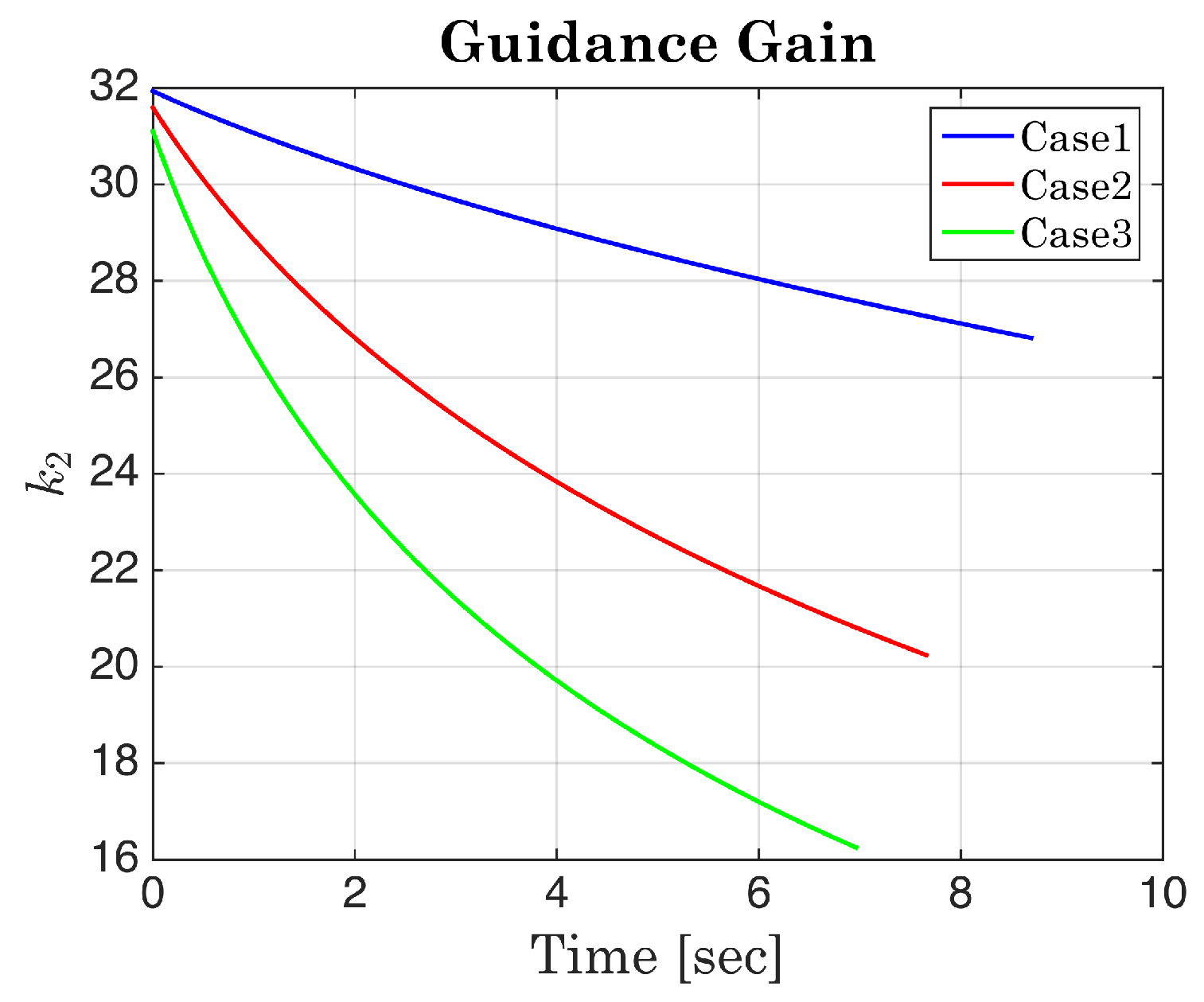
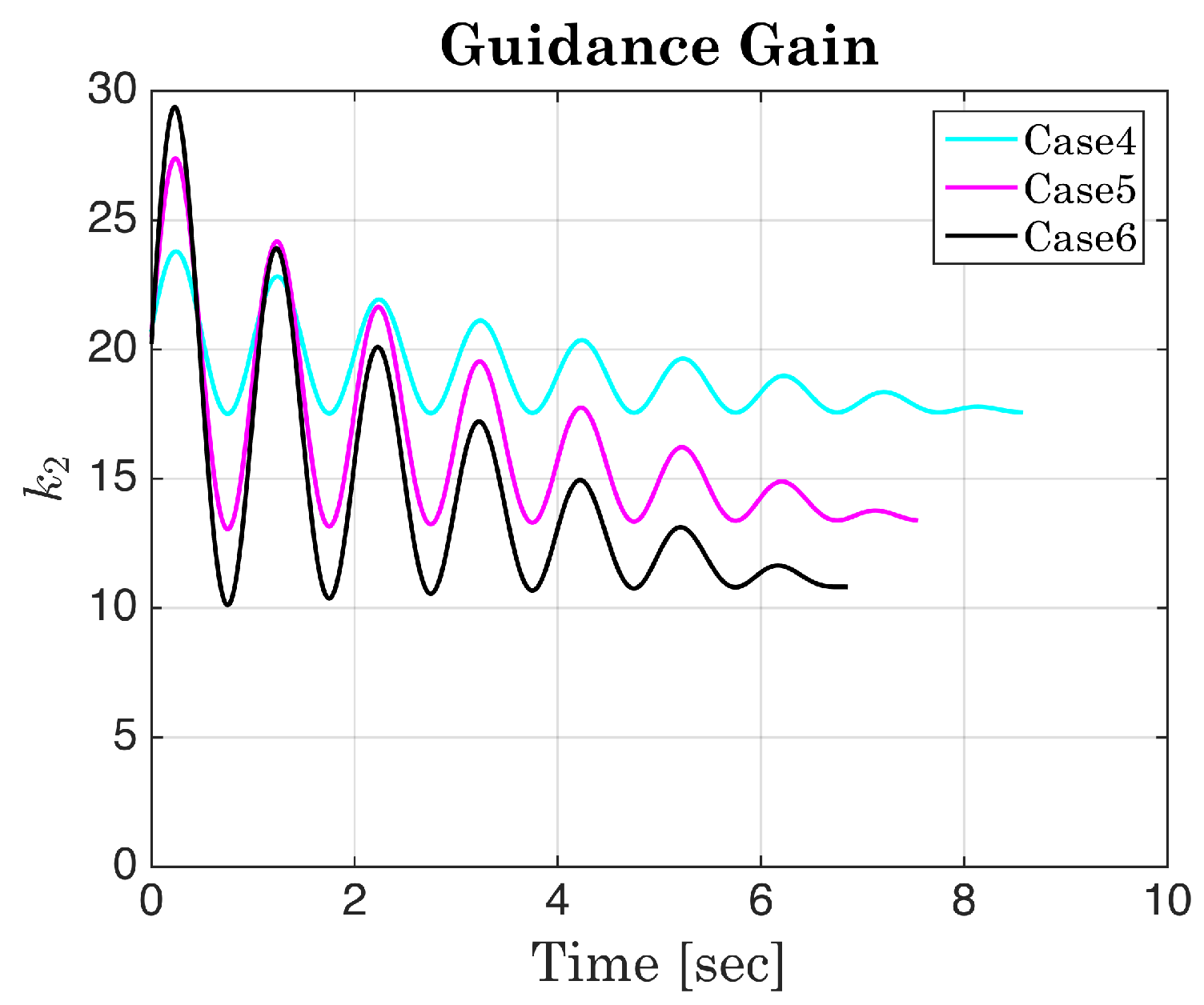
Figure 11 has an oscillation mode, but Figure 10 has no oscillation. This is explained by Figure 12 and Figure 13. Figure 12 shows that speed keeps increasing with a constant slope because of constant thrust. Figure 13 represents continuously increasing speed with an oscillation mode because the time-varying thrust is generated from a 1 Hz sinusoidal function. From (2) and (18), speed and acceleration are employed to produce line-of-sight and flight-path-angle rates. Hence, the 1 Hz frequency mode is included in the heading error calculated by integrating the difference between the line-of-sight and flight-path-angle rates. Figure 14 and Figure 15 represents guidance gains according to thrust. When time goes by, guidance gains decrease. The 1 Hz oscillation mode is included in the guidance-gain profiles of Figure 15 due to feedback information such as acceleration, speed, and heading error.

In real applications, acceleration is measured by sensors such as accelerometers that contain high-frequency noise. We devise three scenario Cases 7–9 by adding measurement noise into time-varying thrust represented by Cases 4–6. The maximum magnitude of measurement noise is assumed to be 20% of the maximum time-varying thrust of each case. The frequency of measurement noise is set to be 20 Hz. Figure 16 and Figure 17 represent all of the trajectories and guidance gains of Cases 4–9, respectively. Although significantly large measurement noise is included in the proposed guidance law, zero miss distance and zero impact-angle error are met in

Table 2. Miss Distance and impact-angle error of Cases 4–9.

Cases	Case 4	Case 5	Case 6	Case 7	Case 8	Case 9
Miss Distance	0.0035 m	0.0103 m	0.0209 m	0.0066 m	0.0083 m	0.0068 m
Angle Error 1	0.0000 deg	−0.0004 deg	−0.0238 deg	0.0000 deg	0.0004 deg	0.0017 deg

¹ This is an impact-angle error.

.

We simulate a biased proportional navigation guidance (BPNG) law practically widely used for an actual UAV application in [2] to compare the proposed guidance law.

Table 3. Miss Distance and impact-angle error of Biased PNG [2].

Cases	Case 1	Case 2	Case 3	Case 4	Case 5	Case 6
Miss Distance	0.0102 m	0.0051 m	0.0176 m	0.0046 m	0.0152 m	0.0088 m
Angle Error 1	−0.4699 deg	−1.4314 deg	−2.0026 deg	−0.4950 deg	−1.4792 deg	−2.0610 deg

¹ This is impact-angle error.

shows the BPNG law simulation results of miss distance and impact-angle error according to the thrust profiles of Cases 1–6. From Table 1 and Table 3, the proposed guidance law and the BPNG law exhibit similar performance in terms of miss distance. However, the impact-angle error of the BPNG law is much larger than that of the proposed guidance law. Therefore, the proposed guidance law is more advantageous than the BPNG law for the time-varying thrust.

6. Conclusions

This paper presents a nonlinear impact-angle guidance law for unmanned aerial vehicles (UAVs) with time-varying thrust. By analytically solving second-order error dynamics with nonlinear time-varying coefficients, we update guidance gains according to initial and current states by real time. This strategy, which is based on an analytic solution, enables one to reduce the dispersion of trajectory. Furthermore, we show that the proposed guidance gains guarantee finite-time error convergence from the Lyapunov stability theory. Future work will deal with various physical constraints such as acceleration constraints.

References

- Chawla, C.; Sarmah, P.; Padhi, R. Suboptimal reentry guidance of a reusable launch vehicle using pitch plane maneuver. Aerosp. Sci. Technol. 2010, 14, 377–386. [Google Scholar] [CrossRef]
- Jeong, S.; Cho, S.; Kim, E. Angle Constraint Biased PNG. In Proceedings of the 2004 5th Asian Control Conference, Melbourne, Australia, 20–23 July 2004; pp. 1849–1854. [Google Scholar]
- Nelson, R.C. Flight Stability and Automatic Control, 2nd ed.; McGraw-Hill: New York, NY, USA, 1998. [Google Scholar]
- Heister, S.D.; Anderson, W.E.; Pourpoint, T.; Cassady, R.J. Rocket Propulsion. Cambridge University Series: Cambridge, UK, 2018. [Google Scholar]
- Zarchan, P. Tactical and Strategic Missile Guidance, 7th ed.; AIAA: Reston, VA, USA, 2019. [Google Scholar]
- Erer, K.; Merttopçuoğlu, O. Indirect impact-angle-control against stationary targets using biased pure proportional navigation. J. Guid. Control Dyn. 2012, 35, 700–704. [Google Scholar] [CrossRef]
- Kim, B.; Lee, J.; Han, H. Biased PNG law for impact with angular constraint. IEEE Trans. Aerosp. Electron. Syst. 1998, 34, 277–288. [Google Scholar]
- Kim, T.; Park, B.; Tahk, M. Bias-shaping method for biased proportional navigation with terminal-angle constraint. J. Guid. Control Dyn. 2013, 36, 1810–1815. [Google Scholar] [CrossRef]
- Shima, T. Intercept-angle guidance. J. Guid. Control Dyn. 2011, 34, 484–492. [Google Scholar] [CrossRef]
- Hari, N.S.B. Impact time and angle guidance with sliding mode control. IEEE Trans. Control Syst. Technol. 2012, 6, 1436–1449. [Google Scholar]
- Kumar, S.; Rao, S.; Ghose, D. Sliding-mode guidance and control for all-aspect interceptors with terminal angle constraints. J. Guid. Control Dyn. 2012, 35, 1230–1246. [Google Scholar] [CrossRef]
- He, S.; Lin, D.; Wang, J. Continuous second-order sliding mode based impact-angle guidance law. Aerosp. Sci. Technol. 2015, 41, 199–208. [Google Scholar] [CrossRef]
- Ryoo, C.K.; Ryoo, C.K.; Tahk, M.J. Optimal Guidance Laws with Terminal Impact Angle Constraint. J. Guid. Control Dyn. 2005, 28, 724–732. [Google Scholar] [CrossRef]
- Lee, Y.; Kim, S.; Tahk, M. Optimality of linear time-varying guidance for impact-angle control. IEEE Trans. Aerosp. Electron. Syst. 2012, 48, 2802–2817. [Google Scholar] [CrossRef]
- Lee, Y.; Ryoo, C.; Kim, E. Optimal guidance with constraints on impact angle and terminal acceleration. In Proceedings of the AIAA Guidance Control Conference Exhibition, Austin, TX, USA, 11–14 August 2003; pp. 11–14. [Google Scholar]
- Shaferman, V.; Shima, T. Cooperative optimal guidance laws for imposing a relative intercept angle. J. Guid. Control Dyn. 2015, 38, 1395–1408. [Google Scholar] [CrossRef]
- Ebrahimia, B.; Bahrami, M.; Roshanianc, J. Optimal sliding-mode guidance with terminal velocity constraint for fixed-interval propulsive maneuvers. Acta Astronaut. 2008, 62, 556–562. [Google Scholar] [CrossRef]
- Cho, H.; Ryoo, C.K. Closed-Form Optimal Guidance Law for Missiles of Time-Varying Velocity. J. Guid. Control Dyn. 1996, 19, 1017–1022. [Google Scholar] [CrossRef]
- Yeh, F.; Chien, H.; Fu, L. Design of Optimal Midcourse Guidance Sliding-Mode Control for Missiles with TVC. IEEE Trans. Aerosp. Electron. Syst. 2003, 39, 824–837. [Google Scholar]
- Seo, M.G.; Tahk, M.J. Suboptimal mid-course guidance algorithm for accelerating missiles. Proc. Inst. Mech. Eng. Part G J. Aerosp. Eng. 2016, 231, 1–16. [Google Scholar] [CrossRef]
- Cheng, Z.; Wang, B.; Liu, L.; Wang, Y. Adaptive Polynomial Guidance With Impact Angle Constraint Under Varying Velocity. IEEE Access 2019, 7, 104210–104217. [Google Scholar] [CrossRef]
- Ye, D.; Tang, X.; Sun, Z.; Wang, C. Multiple model adaptive intercept strategy of spacecraft for an incomplete-information game. Acta Astronaut. 2021, 180, 340–349. [Google Scholar] [CrossRef]
- Hladio, A.; Nielsen, C.; Wang, D. Path Following for a Class of Mechanical Systems. IEEE Trans. Control Syst. Technol. 2013, 21, 2380–2390. [Google Scholar] [CrossRef]
- Yi, B.; Ortega, R.; Manchester, I.R.; Siguerdidjane, H. Path following of a class of underactuated mechanical systems via immersion and invariance-based orbital stabilizationy. Int. J. Robust Nonlinear Control 2020, 30, 8521. [Google Scholar] [CrossRef]
Figure 1.
Guidance geometry.
Figure 2.
Analytic and true solutions (constant thrust scenario).
Figure 3.
Analytic and true solutions (time-varying thrust scenario).
Figure 4.
Thrust profiles of Cases 1–3.
Figure 5.
Thrust profiles of Cases 4–6.
Figure 6.
Trajectories of Cases 1–3.
Figure 7.
Trajectories of Cases 4–6.
Figure 8.
Line-of-sight angle error (constant thrust scenario).
Figure 9.
Line-of-sight angle error (time-varying thrust scenario).
Figure 10.
Heading error (constant thrust scenario).
Figure 11.
Heading error (time-varying thrust scenario).
Figure 12.
Speed profile (constant thrust scenario).
Figure 13.
Speed profile (time-varying thrust scenario).
Figure 14.
Guidance gain (constant thrust scenario).
Figure 15.
Guidance gain (time-varying thrust scenario).
Figure 16.
Trajectories of Case 4–9.
Figure 17.
Guidance gain of Cases 4–9.