
Predicting Subgrade Resistance Value of Hydrated Lime-Activated Rice Husk Ash-Treated Expansive Soil: A Comparison between M5P, Support Vector Machine, and Gaussian Process Regression Algorithms
 , , ,
, , ,  , and
, and
Abstract
:1. Introduction
2. Materials and Methods
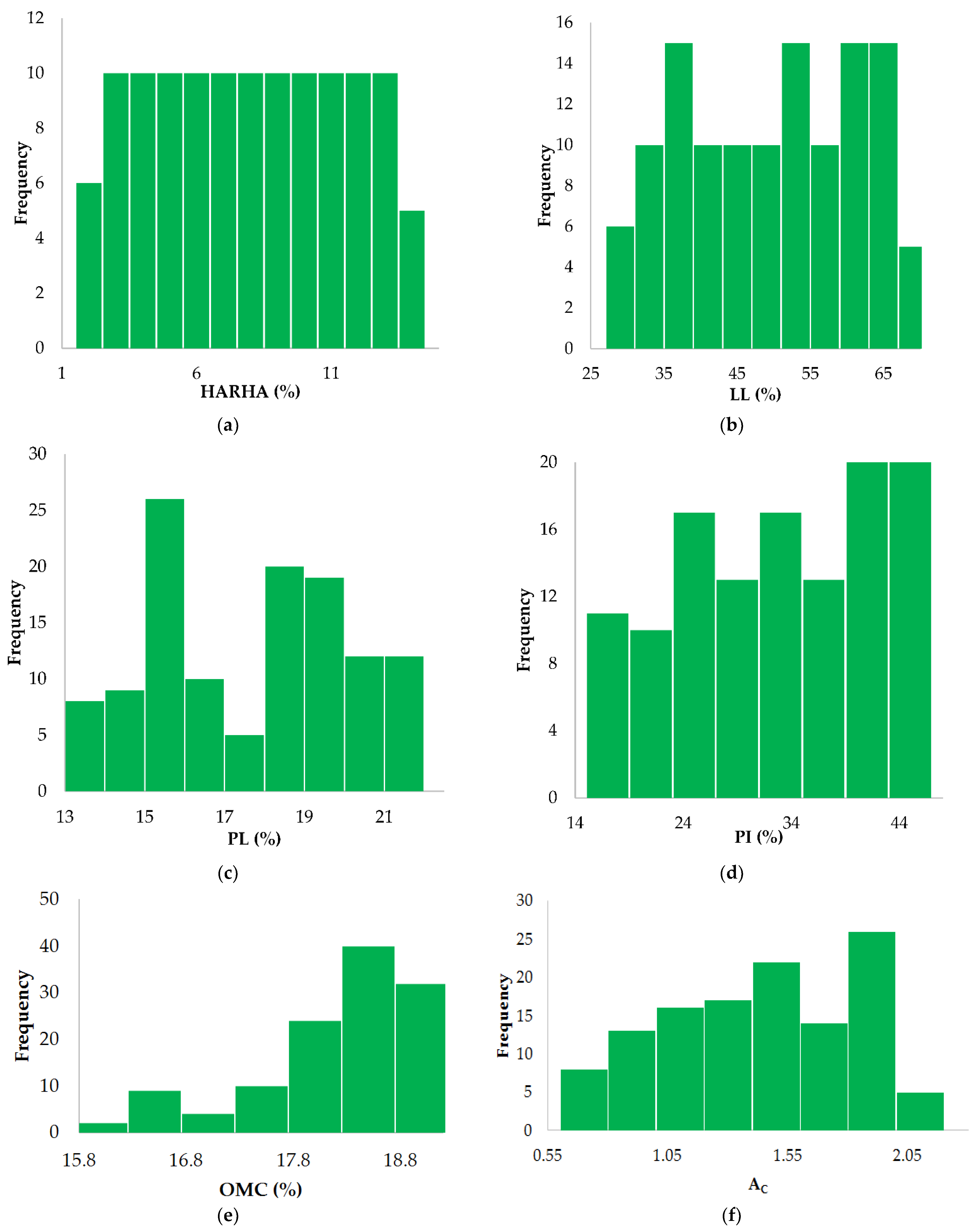
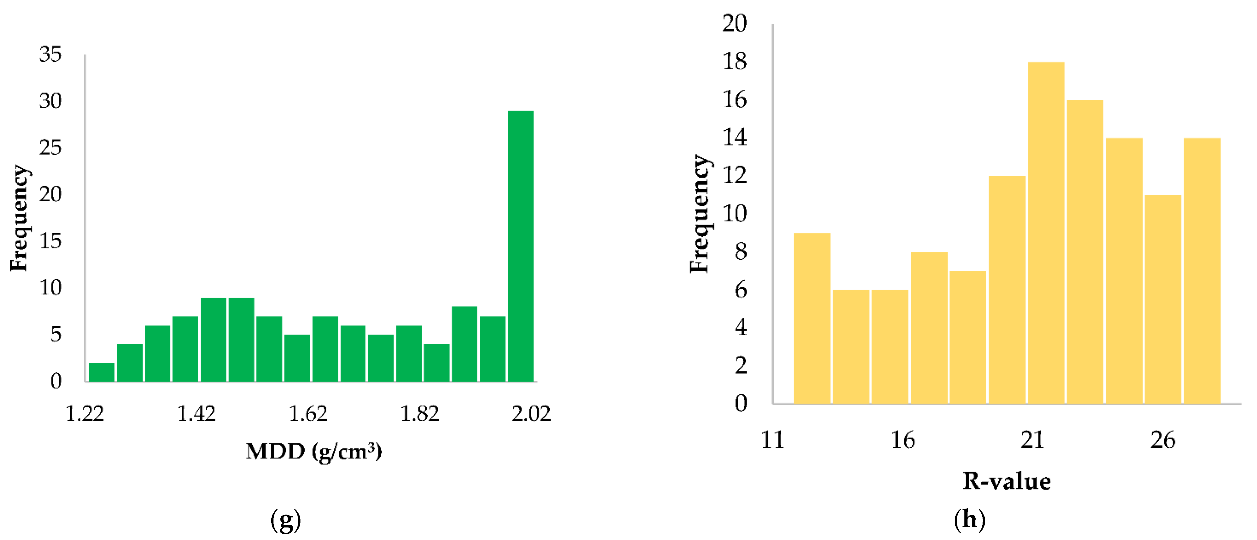
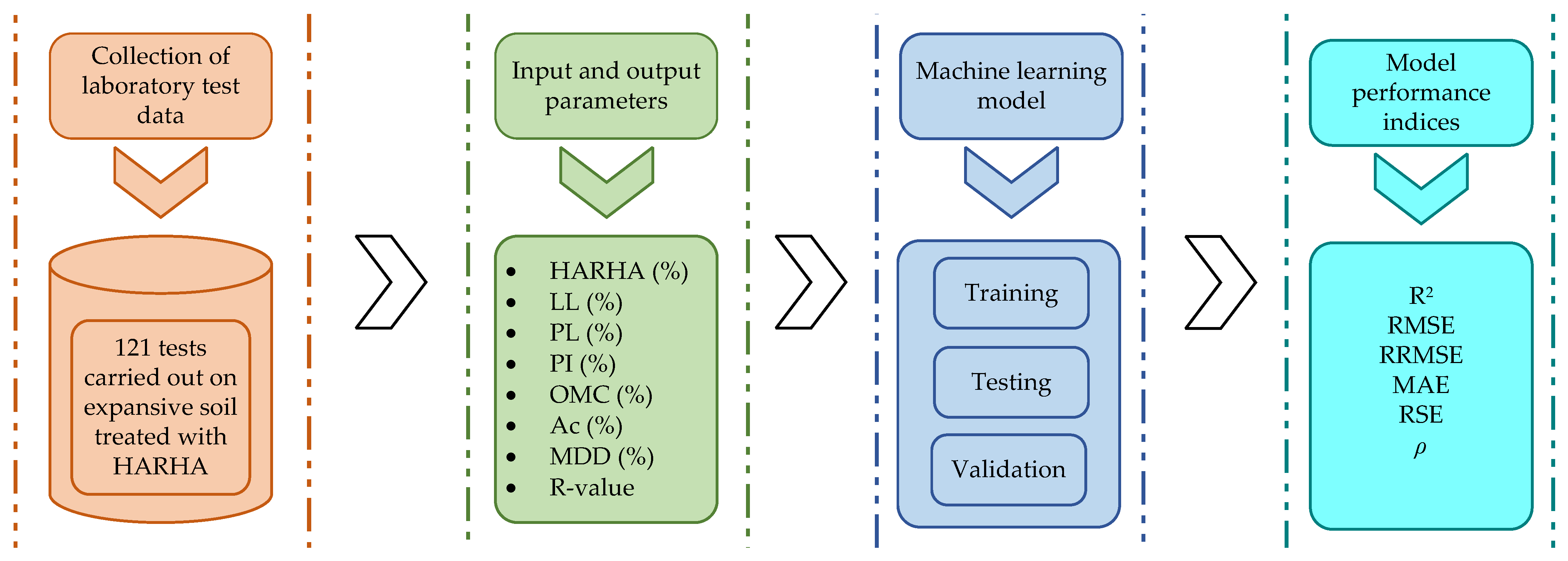
2.1. Data Collection
2.2. Pearson’s Correlation Analysis
2.3. Machine-Learning Algorithms
2.3.1. Gaussian Process Regression (GPR)
2.3.2. M5P
- (i)
- Creating a model tree: Using the dividing criterion, the entered space was divided into numerous subspaces. The predicted error at the node was reduced by applying the standard deviation reduction factor (SDR). The SDR equation is displayed as follows:
- (ii)
- Pruning tree: In each subspace, a classifying and regression tree is introduced to overfit the problem and improves classification performance. Any errors encountered in the learning data will be removed during the pruning process.
- (iii)
- Smoothing step: The nearby linear models may experience abrupt discontinuities as a result of the pruning tree. Therefore, all of the leaf models will be integrated from the leaf to the root to create the final model in order to tackle this problem. The anticipated value is then filtered all the way back to the root. By combining the current value with the expected value from the linear regression, the final value is smoothed using the following equation:where T′ is the predicted value shift to the higher level of the next node, Nt is the predicted value shifted from the lower node to the present node, N is the total number of training instances that shift to the next lower node, A is the predicted value by the node at this node, and K is a constant value.
2.3.3. Support Vector Machine (SVM)
2.4. Model Evaluation and Comparison
3. Results and Analysis
3.1. Hyperparameter Optimization
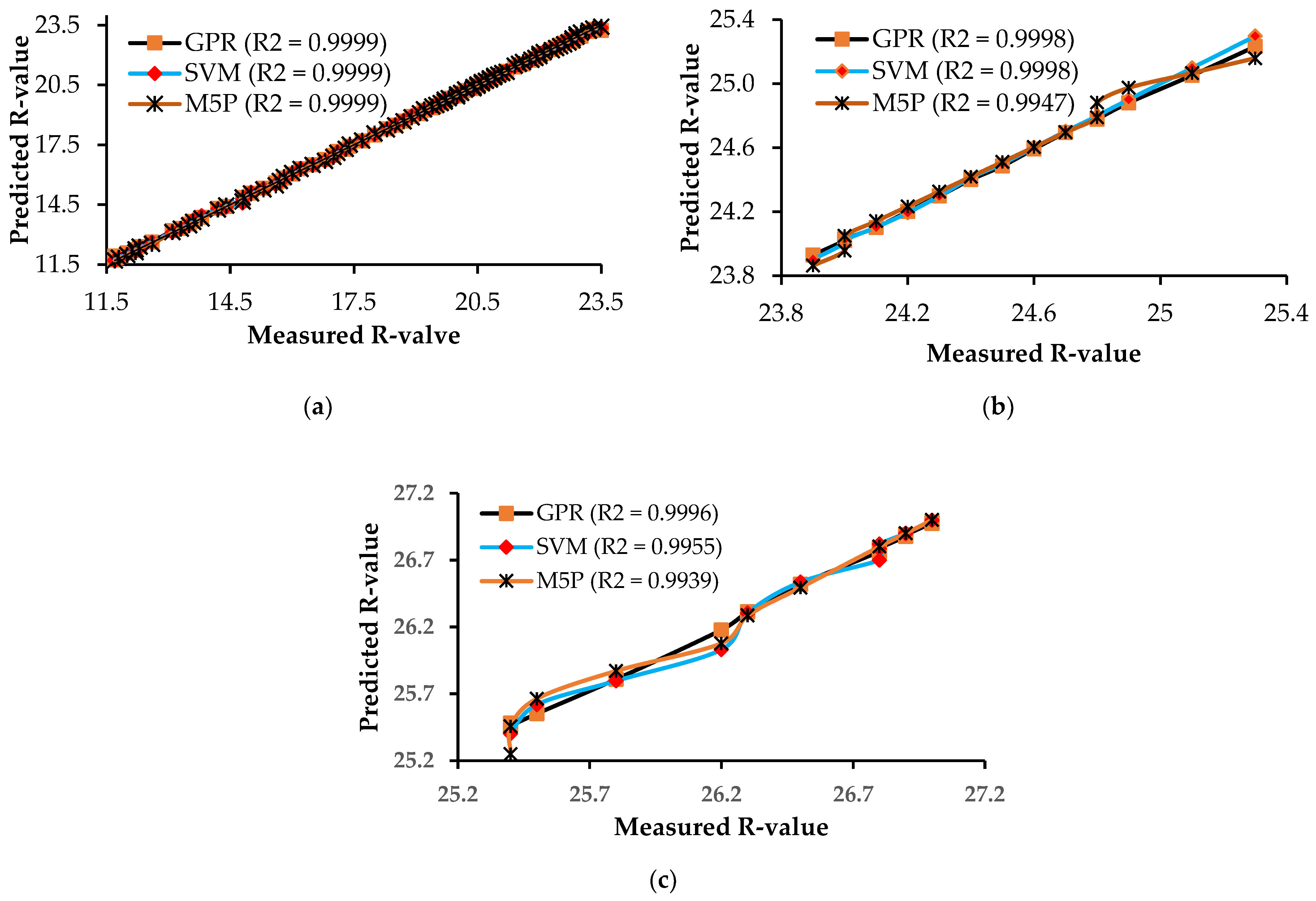
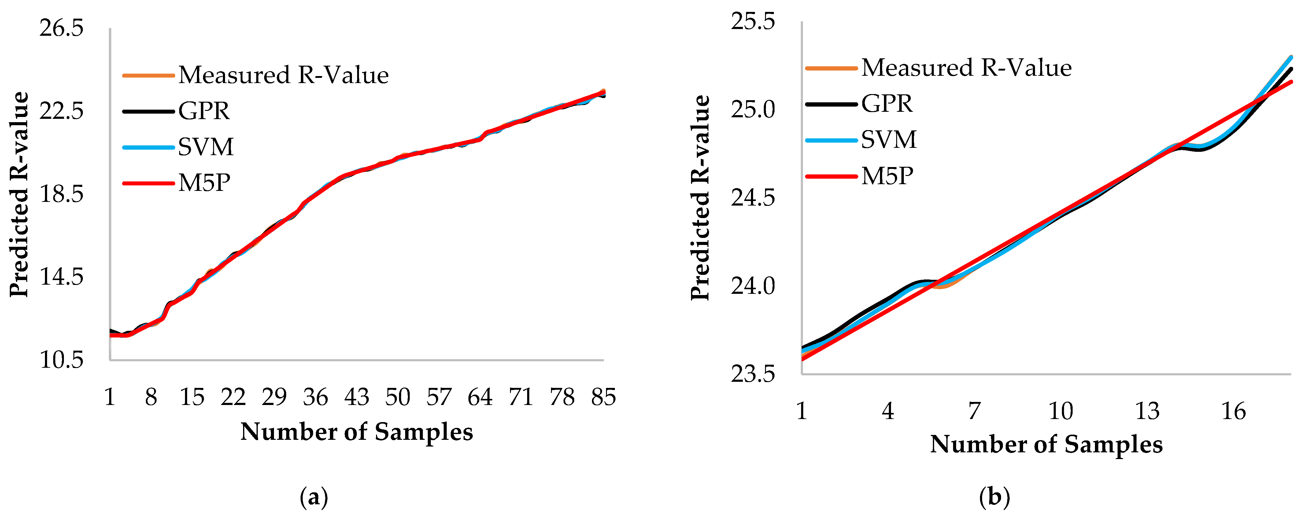
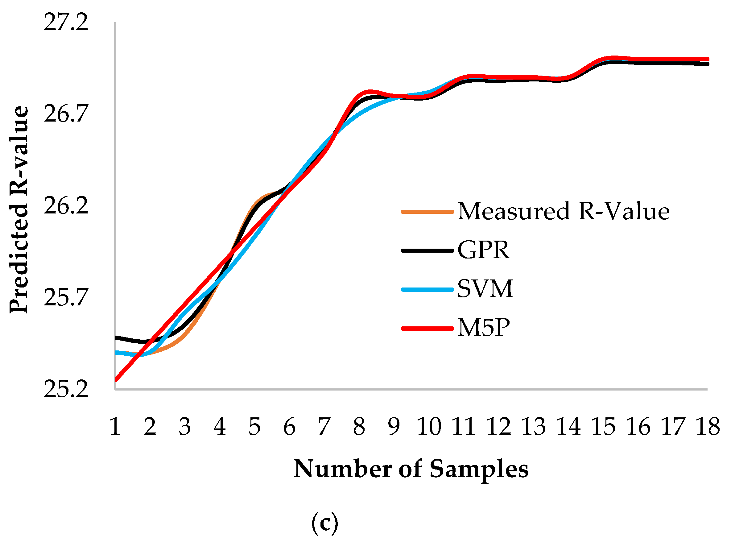
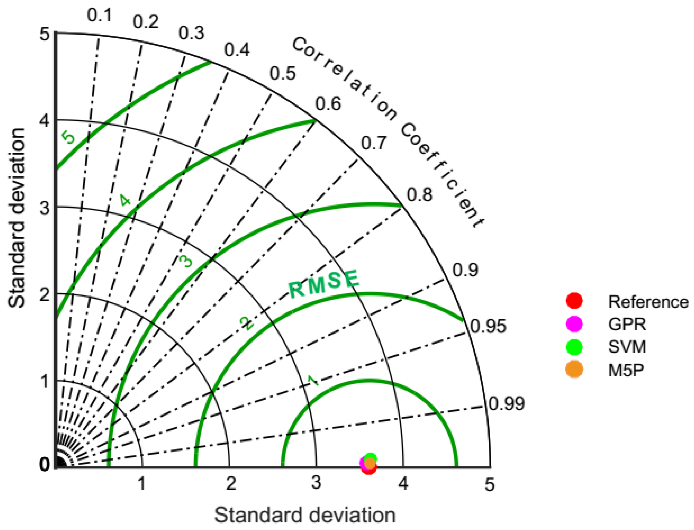
3.2. Model Performance Evaluation
3.3. Rank Analysis
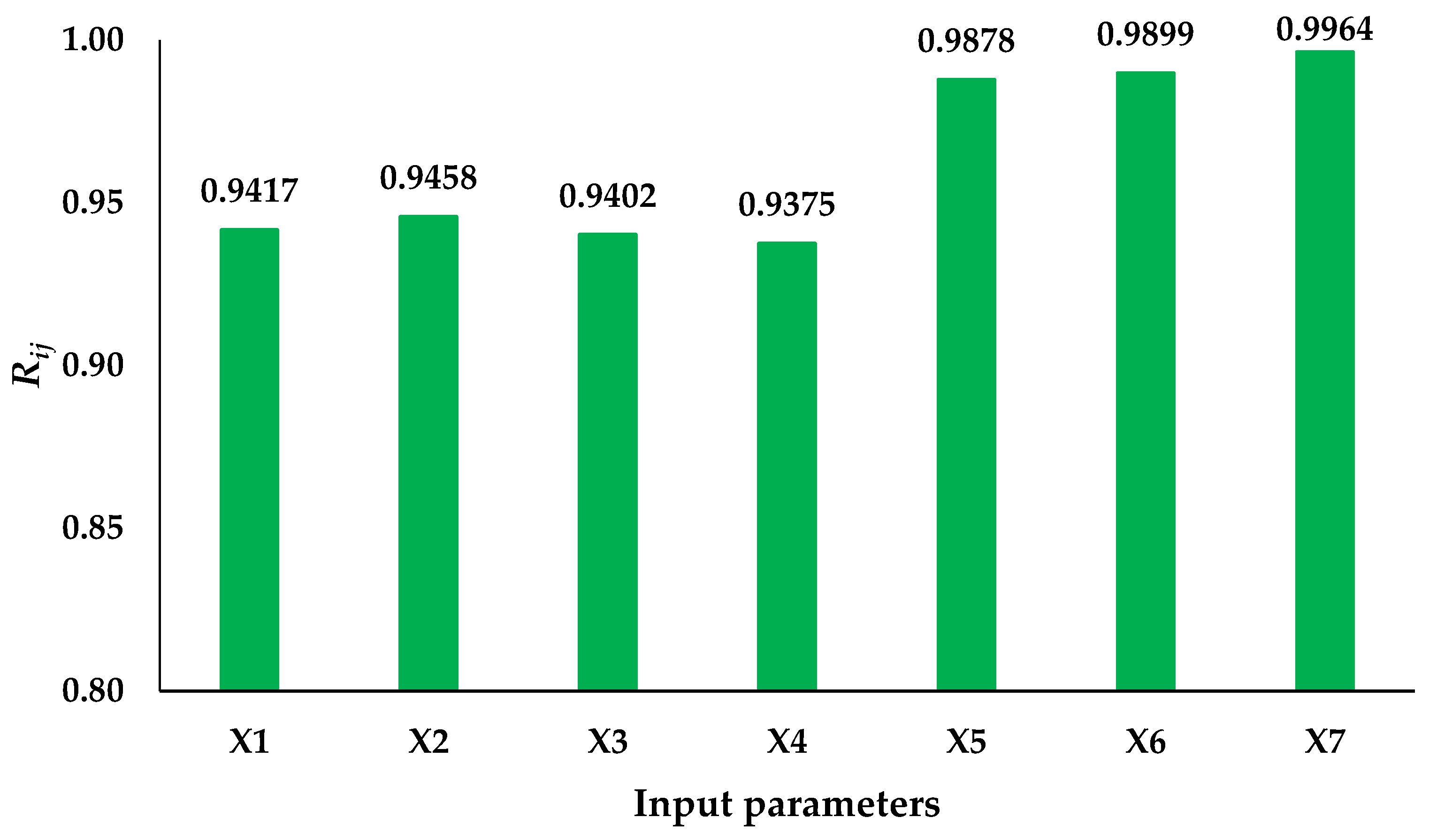
3.4. Sensitivity Analysis
4. Conclusions
Author Contributions
Funding
Data Availability Statement
Acknowledgments
Conflicts of Interest
Appendix A

| S. No. | X1 (%) | X2 (%) | X3 (%) | X4 (%) | X5 (%) | X6 | X7 (g/cm3) | R-value | GPR | M5P | SVM |
|---|---|---|---|---|---|---|---|---|---|---|---|
| 1 | 0 | 66 | 21 | 45 | 16 | 2 | 1.25 | 11.7 | 11.9 | 11.7 | 11.7 |
| 2 | 0.1 | 66 | 21 | 45 | 16 | 1.98 | 1.25 | 11.7 | 11.8 | 11.7 | 11.7 |
| 3 | 0.2 | 65.7 | 20.9 | 44.8 | 16.1 | 1.96 | 1.27 | 11.7 | 11.7 | 11.7 | 11.7 |
| 4 | 0.3 | 65.6 | 20.9 | 44.7 | 16.3 | 1.96 | 1.27 | 11.7 | 11.8 | 11.7 | 11.7 |
| 5 | 0.4 | 65.3 | 20.8 | 44.5 | 16.3 | 1.93 | 1.28 | 11.8 | 11.9 | 11.8 | 11.8 |
| 6 | 0.5 | 65 | 21 | 44 | 16.4 | 1.9 | 1.30 | 12 | 12.1 | 12 | 12 |
| 7 | 0.6 | 64.8 | 20.8 | 44 | 16.4 | 1.88 | 1.31 | 12.2 | 12.2 | 12.1 | 12.2 |
| 8 | 0.7 | 64.5 | 20.8 | 43.7 | 16.45 | 1.88 | 1.31 | 12.2 | 12.2 | 12.3 | 12.2 |
| 9 | 0.8 | 64.1 | 20.8 | 43.3 | 16.47 | 1.87 | 1.33 | 12.3 | 12.4 | 12.4 | 12.4 |
| 10 | 0.9 | 63.5 | 20.9 | 42.6 | 16.49 | 1.85 | 1.33 | 12.6 | 12.6 | 12.5 | 12.6 |
| 11 | 1 | 63 | 21 | 42 | 16.5 | 1.8 | 1.35 | 13.1 | 13.2 | 13.1 | 13.1 |
| 12 | 1.1 | 62.5 | 20.6 | 41.9 | 16.6 | 1.8 | 1.35 | 13.3 | 13.3 | 13.3 | 13.3 |
| 13 | 1.2 | 62.1 | 20.3 | 41.8 | 16.7 | 1.81 | 1.36 | 13.5 | 13.5 | 13.5 | 13.5 |
| 14 | 1.3 | 61.9 | 20.2 | 41.7 | 16.8 | 1.8 | 1.37 | 13.6 | 13.7 | 13.6 | 13.7 |
| 15 | 1.4 | 61.7 | 20.1 | 41.6 | 17 | 1.81 | 1.38 | 13.8 | 13.9 | 13.8 | 13.9 |
| 16 | 1.5 | 61.5 | 20 | 41.5 | 17.2 | 1.8 | 1.38 | 14.2 | 14.3 | 14.2 | 14.3 |
| 17 | 1.6 | 61.4 | 20 | 41.4 | 17.2 | 1.8 | 1.39 | 14.4 | 14.4 | 14.5 | 14.4 |
| 18 | 1.7 | 61.3 | 20 | 41.3 | 17.3 | 1.79 | 1.39 | 14.8 | 14.7 | 14.7 | 14.6 |
| 19 | 1.8 | 61.3 | 20.1 | 41.2 | 17.5 | 1.81 | 1.40 | 14.8 | 14.9 | 14.9 | 14.8 |
| 20 | 1.9 | 61.2 | 20.1 | 41.1 | 17.7 | 1.8 | 1.41 | 15 | 15.1 | 15.1 | 15.1 |
| 21 | 2 | 61 | 20 | 41 | 17.8 | 1.8 | 1.41 | 15.3 | 15.3 | 15.3 | 15.3 |
| 22 | 2.1 | 60.9 | 19.9 | 41 | 17.9 | 1.8 | 1.42 | 15.6 | 15.6 | 15.5 | 15.5 |
| 23 | 2.2 | 60.7 | 19.7 | 41 | 17.9 | 1.8 | 1.42 | 15.7 | 15.7 | 15.7 | 15.6 |
| 24 | 2.3 | 60.6 | 19.6 | 41 | 18 | 1.8 | 1.43 | 15.8 | 15.8 | 15.9 | 15.8 |
| 25 | 2.4 | 60.4 | 19.4 | 41 | 18.2 | 1.8 | 1.43 | 16 | 16 | 16.1 | 16.1 |
| 26 | 2.5 | 60 | 19 | 41 | 18.3 | 1.8 | 1.43 | 16.2 | 16.3 | 16.3 | 16.3 |
| 27 | 2.6 | 59.8 | 19 | 40.8 | 18.35 | 1.79 | 1.44 | 16.5 | 16.5 | 16.5 | 16.5 |
| 28 | 2.7 | 59.7 | 19.1 | 40.6 | 18.4 | 1.77 | 1.45 | 16.8 | 16.8 | 16.7 | 16.7 |
| 29 | 2.8 | 59.5 | 19.1 | 40.4 | 18.45 | 1.75 | 1.46 | 17 | 17 | 16.9 | 16.9 |
| 30 | 2.9 | 59.2 | 19 | 40.2 | 18.5 | 1.72 | 1.46 | 17.1 | 17.2 | 17.1 | 17.1 |
| 31 | 3 | 59 | 19 | 40 | 18.5 | 1.7 | 1.46 | 17.3 | 17.3 | 17.3 | 17.3 |
| 32 | 3.1 | 58.8 | 19.2 | 39.6 | 18.55 | 1.7 | 1.47 | 17.4 | 17.4 | 17.5 | 17.5 |
| 33 | 3.2 | 58.4 | 18.9 | 39.5 | 18.6 | 1.7 | 1.48 | 17.7 | 17.7 | 17.7 | 17.7 |
| 34 | 3.3 | 57.9 | 19.1 | 38.8 | 18.7 | 1.71 | 1.48 | 18 | 18 | 18.1 | 18 |
| 35 | 3.4 | 57.4 | 19 | 38.4 | 18.75 | 1.69 | 1.48 | 18.3 | 18.3 | 18.3 | 18.3 |
| 36 | 3.5 | 57 | 19 | 38 | 18.8 | 1.7 | 1.49 | 18.5 | 18.5 | 18.5 | 18.5 |
| 37 | 3.6 | 56.8 | 18.9 | 37.9 | 18.85 | 1.69 | 1.50 | 18.7 | 18.7 | 18.7 | 18.7 |
| 38 | 3.7 | 56.7 | 19 | 37.7 | 18.9 | 1.65 | 1.51 | 18.9 | 18.9 | 18.9 | 18.9 |
| 39 | 3.8 | 56.5 | 18.9 | 37.6 | 18.93 | 1.64 | 1.51 | 19.1 | 19.1 | 19.1 | 19.1 |
| 40 | 3.9 | 56.3 | 19 | 37.3 | 18.98 | 1.61 | 1.52 | 19.2 | 19.2 | 19.3 | 19.3 |
| 41 | 4 | 56 | 19 | 37 | 19 | 1.6 | 1.52 | 19.4 | 19.4 | 19.4 | 19.4 |
| 42 | 4.1 | 55.7 | 19 | 36.7 | 19 | 1.59 | 1.53 | 19.5 | 19.5 | 19.5 | 19.5 |
| 43 | 4.2 | 54.9 | 18.7 | 36.2 | 19 | 1.57 | 1.54 | 19.6 | 19.6 | 19.6 | 19.6 |
| 44 | 4.3 | 54.1 | 18.5 | 35.6 | 19 | 1.55 | 1.55 | 19.7 | 19.7 | 19.7 | 19.7 |
| 45 | 4.4 | 53.6 | 18.4 | 35.2 | 19 | 1.52 | 1.56 | 19.7 | 19.7 | 19.8 | 19.7 |
| 46 | 4.5 | 53 | 18 | 35 | 19 | 1.5 | 1.57 | 19.8 | 19.8 | 19.8 | 19.8 |
| 47 | 4.6 | 52.8 | 18 | 34.8 | 18.98 | 1.5 | 1.58 | 20 | 19.9 | 19.9 | 19.9 |
| 48 | 4.7 | 52.7 | 18 | 34.7 | 18.96 | 1.5 | 1.59 | 20 | 20 | 20 | 20 |
| 49 | 4.8 | 52.6 | 18.1 | 34.5 | 18.93 | 1.5 | 1.60 | 20.1 | 20.1 | 20.1 | 20.1 |
| 50 | 4.9 | 52.3 | 18 | 34.3 | 18.91 | 1.5 | 1.61 | 20.2 | 20.2 | 20.3 | 20.2 |
| 51 | 5 | 52 | 18 | 34 | 18.9 | 1.5 | 1.61 | 20.4 | 20.3 | 20.3 | 20.3 |
| 52 | 5.1 | 51.5 | 17.7 | 33.8 | 18.88 | 1.48 | 1.62 | 20.4 | 20.4 | 20.4 | 20.4 |
| 53 | 5.2 | 51.1 | 17.7 | 33.4 | 18.86 | 1.46 | 1.63 | 20.5 | 20.5 | 20.5 | 20.5 |
| 54 | 5.3 | 50.8 | 18.1 | 32.7 | 18.84 | 1.43 | 1.64 | 20.5 | 20.5 | 20.5 | 20.5 |
| 55 | 5.4 | 50.3 | 18 | 32.3 | 18.82 | 1.41 | 1.65 | 20.6 | 20.6 | 20.6 | 20.6 |
| 56 | 5.5 | 50 | 18 | 32 | 18.8 | 1.4 | 1.65 | 20.6 | 20.6 | 20.6 | 20.6 |
| 57 | 5.6 | 49.9 | 18 | 31.9 | 18.78 | 1.4 | 1.66 | 20.7 | 20.7 | 20.7 | 20.7 |
| 58 | 5.7 | 49.6 | 17.9 | 31.7 | 18.75 | 1.41 | 1.67 | 20.8 | 20.8 | 20.8 | 20.8 |
| 59 | 5.8 | 49.4 | 17.9 | 31.5 | 18.71 | 1.42 | 1.67 | 20.8 | 20.8 | 20.8 | 20.8 |
| 60 | 5.9 | 49.1 | 17.7 | 31.4 | 18.65 | 1.41 | 1.68 | 20.9 | 20.9 | 20.9 | 20.9 |
| 61 | 6 | 49 | 18 | 31 | 18.6 | 1.4 | 1.69 | 20.9 | 20.9 | 21 | 20.9 |
| 62 | 6.1 | 48.6 | 17.8 | 30.8 | 18.55 | 1.38 | 1.70 | 21 | 21 | 21 | 21 |
| 63 | 6.2 | 48.3 | 17.6 | 30.7 | 18.48 | 1.37 | 1.71 | 21.1 | 21.1 | 21.1 | 21.1 |
| 64 | 6.3 | 47.7 | 17.3 | 30.4 | 18.6 | 1.35 | 1.72 | 21.2 | 21.2 | 21.1 | 21.2 |
| 65 | 6.4 | 47.2 | 17 | 30.2 | 18.44 | 1.33 | 1.73 | 21.4 | 21.4 | 21.5 | 21.4 |
| 66 | 6.5 | 47 | 17 | 30 | 18.4 | 1.3 | 1.74 | 21.5 | 21.5 | 21.6 | 21.5 |
| 67 | 6.6 | 46.8 | 17.1 | 29.7 | 18.4 | 1.31 | 1.75 | 21.6 | 21.6 | 21.7 | 21.6 |
| 68 | 6.7 | 46.5 | 16.8 | 29.7 | 18.41 | 1.31 | 1.76 | 21.8 | 21.7 | 21.8 | 21.7 |
| 69 | 6.8 | 45.6 | 15.9 | 29.7 | 18.4 | 1.3 | 1.77 | 21.9 | 21.8 | 21.9 | 21.9 |
| 70 | 6.9 | 45.2 | 15.9 | 29.3 | 18.41 | 1.3 | 1.78 | 22 | 22 | 21.9 | 22 |
| 71 | 7 | 45 | 16 | 29 | 18.4 | 1.3 | 1.78 | 22 | 22 | 22 | 22.1 |
| 72 | 7.1 | 44.8 | 16.3 | 28.5 | 18.39 | 1.29 | 1.79 | 22.1 | 22.1 | 22.1 | 22.2 |
| 73 | 7.2 | 44.3 | 16.1 | 28.2 | 18.37 | 1.27 | 1.80 | 22.3 | 22.3 | 22.2 | 22.3 |
| 74 | 7.3 | 43.7 | 15.9 | 27.8 | 18.35 | 1.26 | 1.81 | 22.4 | 22.4 | 22.3 | 22.4 |
| 75 | 7.4 | 43.4 | 16 | 27.4 | 18.32 | 1.23 | 1.83 | 22.5 | 22.5 | 22.4 | 22.5 |
| 76 | 7.5 | 43 | 16 | 27 | 18.3 | 1.2 | 1.84 | 22.6 | 22.6 | 22.5 | 22.6 |
| 77 | 7.6 | 42.8 | 15.9 | 26.9 | 18.29 | 1.19 | 1.85 | 22.7 | 22.7 | 22.6 | 22.7 |
| 78 | 7.7 | 42.4 | 16 | 26.4 | 18.28 | 1.18 | 1.86 | 22.8 | 22.7 | 22.7 | 22.8 |
| 79 | 7.8 | 41.8 | 15.4 | 26.4 | 18.26 | 1.16 | 1.87 | 22.8 | 22.8 | 22.8 | 22.8 |
| 80 | 7.9 | 41.5 | 15.4 | 26.1 | 18.23 | 1.14 | 1.87 | 22.9 | 22.9 | 22.9 | 22.9 |
| 81 | 8 | 41 | 15 | 26 | 18.2 | 1.13 | 1.88 | 22.9 | 22.9 | 23 | 22.9 |
| 82 | 8.1 | 40.7 | 14.9 | 25.8 | 18.2 | 1.12 | 1.88 | 23 | 22.9 | 23.1 | 23 |
| 83 | 8.2 | 40.3 | 15 | 25.3 | 18.2 | 1.11 | 1.89 | 23.2 | 23.2 | 23.2 | 23.2 |
| 84 | 8.3 | 39.8 | 15.1 | 24.7 | 18.2 | 1.11 | 1.90 | 23.3 | 23.3 | 23.3 | 23.3 |
| 85 | 8.4 | 39.3 | 15 | 24.3 | 18.21 | 1.1 | 1.90 | 23.5 | 23.2 | 23.4 | 23.4 |
| 86 | 8.5 | 39 | 15 | 24 | 18.2 | 1 | 1.91 | 23.6 | 23.6 | 23.6 | 23.6 |
| 87 | 8.6 | 38.8 | 15 | 23.8 | 18.2 | 1 | 1.92 | 23.7 | 23.7 | 23.7 | 23.7 |
| 88 | 8.7 | 38.3 | 14.9 | 23.4 | 18.2 | 1 | 1.93 | 23.8 | 23.8 | 23.8 | 23.8 |
| 89 | 8.8 | 37.9 | 15.2 | 22.7 | 18.2 | 1 | 1.94 | 23.9 | 23.9 | 23.9 | 23.9 |
| 90 | 8.9 | 37.5 | 15.2 | 22.3 | 18.2 | 1 | 1.95 | 24 | 24 | 24 | 24 |
| 91 | 9 | 37 | 15 | 22 | 18.2 | 1 | 1.96 | 24 | 24 | 24 | 24 |
| 92 | 9.1 | 37 | 15 | 22 | 18.19 | 1 | 1.96 | 24.1 | 24.1 | 24.1 | 24.1 |
| 93 | 9.2 | 37 | 15 | 22 | 18.18 | 1 | 1.96 | 24.2 | 24.2 | 24.2 | 24.2 |
| 94 | 9.3 | 37 | 15 | 22 | 18.16 | 1 | 1.97 | 24.3 | 24.3 | 24.3 | 24.3 |
| 95 | 9.4 | 37 | 15 | 22 | 18.13 | 1 | 1.97 | 24.4 | 24.4 | 24.4 | 24.4 |
| 96 | 9.5 | 37 | 15 | 22 | 18.1 | 1 | 1.97 | 24.5 | 24.5 | 24.5 | 24.5 |
| 97 | 9.6 | 36.8 | 15.1 | 21.7 | 18 | 0.99 | 1.97 | 24.6 | 24.6 | 24.6 | 24.6 |
| 98 | 9.7 | 36.7 | 15.1 | 21.6 | 17.92 | 0.98 | 1.97 | 24.7 | 24.7 | 24.7 | 24.7 |
| 99 | 9.8 | 36.5 | 15.1 | 21.4 | 17.93 | 0.97 | 1.98 | 24.8 | 24.8 | 24.8 | 24.8 |
| 100 | 9.9 | 36.3 | 15.2 | 21.1 | 17.91 | 0.94 | 1.98 | 24.8 | 24.8 | 24.9 | 24.8 |
| 101 | 10 | 36 | 15 | 21 | 17.9 | 0.9 | 1.98 | 24.9 | 24.9 | 25 | 24.9 |
| 102 | 10.1 | 35.7 | 14.9 | 20.8 | 17.88 | 0.88 | 1.98 | 25.1 | 25.1 | 25.1 | 25.1 |
| 103 | 10.2 | 35.5 | 15.1 | 20.4 | 17.84 | 0.86 | 1.98 | 25.3 | 25.2 | 25.2 | 25.3 |
| 104 | 10.3 | 34.6 | 14.9 | 19.7 | 17.79 | 0.84 | 1.98 | 25.4 | 25.5 | 25.3 | 25.4 |
| 105 | 10.4 | 33.3 | 14 | 19.3 | 17.73 | 0.82 | 1.99 | 25.4 | 25.5 | 25.5 | 25.4 |
| 106 | 10.5 | 33 | 14 | 19 | 17.7 | 0.8 | 1.99 | 25.5 | 25.6 | 25.7 | 25.6 |
| 107 | 10.6 | 32.8 | 14 | 18.8 | 17.7 | 0.79 | 1.99 | 25.8 | 25.8 | 25.9 | 25.8 |
| 108 | 10.7 | 32.4 | 13.9 | 18.5 | 17.71 | 0.78 | 1.99 | 26.2 | 26.2 | 26.1 | 26 |
| 109 | 10.8 | 31.5 | 13.9 | 17.6 | 17.71 | 0.75 | 1.99 | 26.3 | 26.3 | 26.3 | 26.3 |
| 110 | 10.9 | 31.1 | 14 | 17.1 | 17.7 | 0.72 | 1.99 | 26.5 | 26.5 | 26.5 | 26.5 |
| 111 | 11 | 31 | 14 | 17 | 17.7 | 0.7 | 1.99 | 26.8 | 26.8 | 26.8 | 26.7 |
| 112 | 11.1 | 30.7 | 13.9 | 16.8 | 17.68 | 0.7 | 1.99 | 26.8 | 26.8 | 26.8 | 26.8 |
| 113 | 11.2 | 30.3 | 13.7 | 16.6 | 17.63 | 0.71 | 1.99 | 26.8 | 26.8 | 26.8 | 26.8 |
| 114 | 11.3 | 29.8 | 13.4 | 16.4 | 17.57 | 0.71 | 1.99 | 26.9 | 26.9 | 26.9 | 26.9 |
| 115 | 11.4 | 29.4 | 13.2 | 16.2 | 17.53 | 0.71 | 1.98 | 26.9 | 26.9 | 26.9 | 26.9 |
| 116 | 11.5 | 29 | 13 | 16 | 17.5 | 0.7 | 1.97 | 26.9 | 26.9 | 26.9 | 26.9 |
| 117 | 11.6 | 28.7 | 12.8 | 15.9 | 17.5 | 0.69 | 1.97 | 26.9 | 26.9 | 26.9 | 26.9 |
| 118 | 11.7 | 28.5 | 13 | 15.5 | 17.4 | 0.67 | 1.96 | 27 | 27 | 27 | 27 |
| 119 | 11.8 | 27.8 | 13 | 14.8 | 17.3 | 0.65 | 1.96 | 27 | 27 | 27 | 27 |
| 120 | 11.9 | 27.6 | 13.2 | 14.4 | 17.2 | 0.62 | 1.95 | 27 | 27 | 27 | 27 |
| 121 | 12 | 27 | 13 | 14 | 17.1 | 0.6 | 1.95 | 27 | 27 | 27 | 27 |
References
- American Association of State Highway and Transportation Officials (AASHTO). Standard Method of Test for Resistance R-Value and Expansion Pressure of Compacted Soils; Transportation Research Board: Washington, DC, USA, 2002. [Google Scholar]
- Bandara, N.; Rowe, G.M. Design subgrade resilient modulus for Florida subgrade soils. In Resilient Modulus Testing for Pavement Components; ASTM International: West Conshohocken, PA, USA, 2003. [Google Scholar]
- Khazanovich, L.; Celauro, C.; Chadbourn, B.; Zollars, J.; Dai, S. Evaluation of subgrade resilient modulus predictive model for use in mechanistic–empirical pavement design guide. Transp. Res. Rec. 2006, 1947, 155–166. [Google Scholar] [CrossRef]
- Onyelowe, K.C.; Onyia, M.E.; Onyelowe, F.D.A.; Van, D.B.; Salahudeen, A.B.; Eberemu, A.O.; Osinubi, K.J.; Amadi, A.A.; Onukwugha, E.; Odumade, A.O. Critical state desiccation induced shrinkage of biomass treated compacted soil as pavement foundation. Építöanyag 2020, 72, 40–47. [Google Scholar] [CrossRef]
- Onyelowe, K.C.; Bui Van, D.; Ubachukwu, O.; Ezugwu, C.; Salahudeen, B.; Nguyen Van, M.; Ikeagwuani, C.; Amhadi, T.; Sosa, F.; Wu, W. Recycling and reuse of solid wastes; a hub for ecofriendly, ecoefficient and sustainable soil, concrete, wastewater and pavement reengineering. Int. J. Low-Carbon Technol. 2019, 14, 440–451. [Google Scholar] [CrossRef]
- Tarefder, R.A.; Saha, N.; Hall, J.W.; Ng, P.T. Evaluating weak subgrade for pavement design and performance prediction: A case study of US 550. J. GeoEngineer. 2008, 3, 13–24. [Google Scholar]
- Rehman, Z.; Khalid, U.; Farooq, K.; Mujtaba, H. Prediction of CBR value from index properties of different soils. Technol. J. Univ. Eng. Technol. (UET) 2017, 22, 17–26. [Google Scholar]
- Officials, T. New Mexico Department of Transportation (NMDOT), Standard Specifications for Highway and Bridge Construction. Section 200–600, New Mexico DOT; Aashto: Washington, DC, USA, 2004. [Google Scholar]
- Kişi, Ö.; Uncuoğlu, E. Comparison of three back-propagation training algorithms for two case studies. Indian J. Eng. Mater. Sci. 2005, 12, 434–442. [Google Scholar]
- Van, D.B.; Onyelowe, K.C.; Van-Nguyen, M. Capillary rise, suction (absorption) and the strength development of HBM treated with QD base geopolymer. Int. J. Pavement Res. Technol. 2018, 4, 759–765. [Google Scholar]
- Onyelowe, K.C.; Iqbal, M.; Jalal, F.E.; Onyia, M.E.; Onuoha, I.C. Application of 3-algorithm ANN programming to predict the strength performance of hydrated-lime activated rice husk ash treated soil. Multiscale Multidiscip. Modeling Exp. Des. 2021, 4, 259–274. [Google Scholar] [CrossRef]
- Froemelt, A.; Dürrenmatt, D.J.; Hellweg, S. Using data mining to assess environmental impacts of household consumption behaviors. Environ. Sci. Technol. 2018, 52, 8467–8478. [Google Scholar] [CrossRef]
- Ahmad, M.; Tang, X.-W.; Qiu, J.-N.; Gu, W.-J.; Ahmad, F. A hybrid approach for evaluating CPT-based seismic soil liquefaction potential using Bayesian belief networks. J. Cent. South Univ. 2020, 27, 500–516. [Google Scholar]
- Ahmad, M.; Tang, X.-W.; Qiu, J.-N.; Ahmad, F. Evaluating seismic soil liquefaction potential using bayesian belief network and C4. 5 decision tree approaches. Appl. Sci. 2019, 9, 4226. [Google Scholar] [CrossRef]
- Ahmad, M.; Tang, X.; Qiu, J.; Ahmad, F.; Gu, W. LLDV-a Comprehensive Framework for Assessing the Effects of Liquefaction Land Damage Potential. In Proceedings of the 2019 IEEE 14th International Conference on Intelligent Systems and Knowledge Engineering (ISKE), Dalian, China, 14–16 November 2019; pp. 527–533. [Google Scholar]
- Ahmad, M.; Tang, X.-W.; Qiu, J.-N.; Ahmad, F.; Gu, W.-J. A step forward towards a comprehensive framework for assessing liquefaction land damage vulnerability: Exploration from historical data. Front. Struct. Civ. Eng. 2020, 14, 1476–1491. [Google Scholar] [CrossRef]
- Ahmad, M.; Tang, X.; Ahmad, F. Evaluation of Liquefaction-Induced Settlement Using Random Forest and REP Tree Models: Taking Pohang Earthquake as a Case of Illustration. In Natural Hazards-Impacts, Adjustments & Resilience; IntechOpen: London, UK, 2020. [Google Scholar]
- Ahmad, M.; Al-Shayea, N.A.; Tang, X.-W.; Jamal, A.; M Al-Ahmadi, H.; Ahmad, F. Predicting the Pillar Stability of Underground Mines with Random Trees and C4. 5 Decision Trees. Appl. Sci. 2020, 10, 6486. [Google Scholar] [CrossRef]
- Ahmad, M.; Kamiński, P.; Olczak, P.; Alam, M.; Iqbal, M.J.; Ahmad, F.; Sasui, S.; Khan, B.J. Development of Prediction Models for Shear Strength of Rockfill Material Using Machine Learning Techniques. Appl. Sci. 2021, 11, 6167. [Google Scholar] [CrossRef]
- Noori, A.M.; Mikaeil, R.; Mokhtarian, M.; Haghshenas, S.S.; Foroughi, M. Feasibility of intelligent models for prediction of utilization factor of TBM. Geotech. Geol. Eng. 2020, 38, 3125–3143. [Google Scholar] [CrossRef]
- Dormishi, A.; Ataei, M.; Mikaeil, R.; Khalokakaei, R.; Haghshenas, S.S. Evaluation of gang saws’ performance in the carbonate rock cutting process using feasibility of intelligent approaches. Eng. Sci. Technol. Int. J. 2019, 22, 990–1000. [Google Scholar] [CrossRef]
- Mikaeil, R.; Haghshenas, S.S.; Hoseinie, S.H. Rock penetrability classification using artificial bee colony (ABC) algorithm and self-organizing map. Geotech. Geol. Eng. 2018, 36, 1309–1318. [Google Scholar] [CrossRef]
- Mikaeil, R.; Haghshenas, S.S.; Ozcelik, Y.; Gharehgheshlagh, H.H. Performance evaluation of adaptive neuro-fuzzy inference system and group method of data handling-type neural network for estimating wear rate of diamond wire saw. Geotech. Geol. Eng. 2018, 36, 3779–3791. [Google Scholar] [CrossRef]
- Momeni, E.; Nazir, R.; Armaghani, D.J.; Maizir, H. Prediction of pile bearing capacity using a hybrid genetic algorithm-based ANN. Measurement 2014, 57, 122–131. [Google Scholar] [CrossRef]
- Xie, C.; Nguyen, H.; Choi, Y.; Armaghani, D.J. Optimized functional linked neural network for predicting diaphragm wall deflection induced by braced excavations in clays. Geosci. Front. 2022, 13, 101313. [Google Scholar] [CrossRef]
- Armaghani, D.J.; Mohamad, E.T.; Narayanasamy, M.S.; Narita, N.; Yagiz, S. Development of hybrid intelligent models for predicting TBM penetration rate in hard rock condition. Tunnel. Undergr. Space Technol. 2017, 63, 29–43. [Google Scholar] [CrossRef]
- Guido, G.; Haghshenas, S.S.; Haghshenas, S.S.; Vitale, A.; Gallelli, V.; Astarita, V. Development of a binary classification model to assess safety in transportation systems using GMDH-type neural network algorithm. Sustainability 2020, 12, 6735. [Google Scholar] [CrossRef]
- Morosini, A.F.; Haghshenas, S.S.; Haghshenas, S.S.; Choi, D.Y.; Geem, Z.W. Sensitivity Analysis for Performance Evaluation of a Real Water Distribution System by a Pressure Driven Analysis Approach and Artificial Intelligence Method. Water 2021, 13, 1116. [Google Scholar] [CrossRef]
- Asteris, P.G.; Lourenço, P.B.; Roussis, P.C.; Adami, C.E.; Armaghani, D.J.; Cavaleri, L.; Chalioris, C.E.; Hajihassani, M.; Lemonis, M.E.; Mohammed, A.S. Revealing the nature of metakaolin-based concrete materials using artificial intelligence techniques. Constr. Build. Mater. 2022, 322, 126500. [Google Scholar] [CrossRef]
- Hajihassani, M.; Armaghani, D.J.; Sohaei, H.; Mohamad, E.T.; Marto, A. Prediction of airblast-overpressure induced by blasting using a hybrid artificial neural network and particle swarm optimization. Appl. Acoust. 2014, 80, 57–67. [Google Scholar] [CrossRef]
- Onyelowe, K.C.; Jalal, F.E.; Onyia, M.E.; Onuoha, I.C.; Alaneme, G.U. Application of gene expression programming to evaluate strength characteristics of hydrated-lime-activated rice husk ash-treated expansive soil. Appl. Comput. Intell. Soft Comput. 2021, 2021, 6686347. [Google Scholar] [CrossRef]
- Onyelowe, K.; Salahudeen, A.B.; Eberemu, A.; Ezugwu, C.; Amhadi, T.; Alaneme, G. Oxides of carbon entrapment for environmental friendly geomaterials ash derivation. In International Congress and Exhibition “Sustainable Civil Infrastructures”; Springer: Berlin/Heidelberg, Germany, 2019; pp. 58–67. [Google Scholar]
- Benesty, J.; Chen, J.; Huang, Y.; Cohen, I. Pearson correlation coefficient. In Noise Reduction in Speech Processing; Springer: Berlin/Heidelberg, Germany, 2009; pp. 1–4. [Google Scholar]
- van Vuren, T. Modeling of transport demand–analyzing, calculating, and forecasting transport demand: By V. A. Profillidis and G. N. Botzoris, Amsterdam, Elsevier, 2018, 472 pp., $125 (paperback and ebook), eBook ISBN: 9780128115145, Paperback ISBN: 9780128115138. Transp. Rev. 2019, 40, 1–2. [Google Scholar] [CrossRef]
- Black, W. A method of estimating the California bearing ratio of cohesive soils from plasticity data. Geotechnique 1962, 12, 271–282. [Google Scholar] [CrossRef]
- Wang, J. An intuitive tutorial to Gaussian processes regression. arXiv 2020, arXiv:2009.10862. [Google Scholar]
- Cheng, M.-Y.; Huang, C.-C.; Roy, A.F.V. Predicting project success in construction using an evolutionary Gaussian process inference model. J. Civ. Eng. Manag. 2013, 19, S202–S211. [Google Scholar] [CrossRef]
- Chou, J.-S.; Chiu, C.-K.; Farfoura, M.; Al-Taharwa, I. Optimizing the prediction accuracy of concrete compressive strength based on a comparison of data-mining techniques. J. Comput. Civ. Eng. 2011, 25, 242–253. [Google Scholar] [CrossRef]
- Mahesh, P.; Deswal, S. Modelling pile capacity using gaussian process regression. Comput. Geotech. 2010, 37, 942–947. [Google Scholar]
- Rasmussen, C.E. Gaussian processes in machine learning. In Summer School on Machine Learning; Springer: Berlin/Heidelberg, Germany, 2003; pp. 63–71. [Google Scholar]
- Wang, Y.; Witten, I.H. Induction of Model Trees for Predicting Continuous Classes; University of Waikato, Department of Computer Science: Hamilton, New Zealand, 1996. [Google Scholar]
- Quinlan, J.R. Learning with continuous classes. In Proceedings of the 5th Australian Joint Conference on Artificial Intelligence, Ai’92, Hobart, Australia, 16–18 November 1992; World Scientific: Singapore, 1992; pp. 343–348. [Google Scholar]
- Tong, S.; Koller, D. Support vector machine active learning with applications to text classification. J. Mach. Learn. Res. 2001, 2, 45–66. [Google Scholar]
- Asefa, T.; Kemblowski, M.; Urroz, G.; McKee, M. Support vector machines (SVMs) for monitoring network design. Groundwater 2005, 43, 413–422. [Google Scholar] [CrossRef]
- Deka, P.C. Support vector machine applications in the field of hydrology: A review. Appl. Soft Comput. 2014, 19, 372–386. [Google Scholar]
- Nguyen, L. Tutorial on support vector machine. Appl. Comput. Math. 2017, 6, 1–15. [Google Scholar]
- Ahmad, M.; Ahmad, F.; Wróblewski, P.; Al-Mansob, R.A.; Olczak, P.; Kamiński, P.; Safdar, M.; Rai, P. Prediction of ultimate bearing capacity of shallow foundations on cohesionless soils: A gaussian process regression approach. Appl. Sci. 2021, 11, 10317. [Google Scholar] [CrossRef]
- Despotovic, M.; Nedic, V.; Despotovic, D.; Cvetanovic, S. Evaluation of empirical models for predicting monthly mean horizontal diffuse solar radiation. Renew. Sustain. Energy Rev. 2016, 56, 246–260. [Google Scholar] [CrossRef]
- Gandomi, A.H.; Roke, D.A. Assessment of artificial neural network and genetic programming as predictive tools. Adv. Eng. Softw. 2015, 88, 63–72. [Google Scholar] [CrossRef]
- Faul, S.; Gregorcic, G.; Boylan, G.; Marnane, W.; Lightbody, G.; Connolly, S. Gaussian process modeling of EEG for the detection of neonatal seizures. IEEE Trans. Biomed. Eng. 2007, 54, 2151–2162. [Google Scholar] [CrossRef]
- Tao, Z.; Huiling, L.; Wenwen, W.; Xia, Y. GA-SVM based feature selection and parameter optimization in hospitalization expense modeling. Appl. Soft Comput. 2019, 75, 323–332. [Google Scholar] [CrossRef]
- Yin, X.; Hou, Y.; Yin, J.; Li, C. A novel SVM parameter tuning method based on advanced whale optimization algorithm. J. Phys. Conf. Ser. 2019, 1237, 022140. [Google Scholar] [CrossRef]
- Ma, J.; Kim, H.M. Continuous preference trend mining for optimal product design with multiple profit cycles. J. Mech. Des. 2014, 136, 061002. [Google Scholar] [CrossRef]
- Mijwel, M.M. Artificial Neural Networks Advantages and Disadvantages. 2018. Available online: https://www.linkedin.com/pulse/artificial-NeuralNetwork (accessed on 15 May 2022).
- Zorlu, K.; Gokceoglu, C.; Ocakoglu, F.; Nefeslioglu, H.; Acikalin, S. Prediction of uniaxial compressive strength of sandstones using petrography-based models. Eng. Geol. 2008, 96, 141–158. [Google Scholar] [CrossRef]
- Wu, X.; Kumar, V. The Top Ten Algorithms in Data Mining; CRC Press: Boca Raton, FL, USA, 2009. [Google Scholar]
- Momeni, E.; Armaghani, D.J.; Hajihassani, M.; Amin, M.F.M. Prediction of uniaxial compressive strength of rock samples using hybrid particle swarm optimization-based artificial neural networks. Measurement 2015, 60, 50–63. [Google Scholar] [CrossRef]
- Faradonbeh, R.S.; Armaghani, D.J.; Abd Majid, M.; Tahir, M.M.; Murlidhar, B.R.; Monjezi, M.; Wong, H. Prediction of ground vibration due to quarry blasting based on gene expression programming: A new model for peak particle velocity prediction. Int. J. Environ. Sci. Technol. 2016, 13, 1453–1464. [Google Scholar] [CrossRef]
- Chen, W.; Hasanipanah, M.; Rad, H.N.; Armaghani, D.J.; Tahir, M. A new design of evolutionary hybrid optimization of SVR model in predicting the blast-induced ground vibration. Eng. Comput. 2019, 37, 1455–1471. [Google Scholar] [CrossRef]
- Rad, H.N.; Bakhshayeshi, I.; Jusoh, W.A.W.; Tahir, M.; Foong, L.K. Prediction of flyrock in mine blasting: A new computational intelligence approach. Nat. Resour. Res. 2020, 29, 609–623. [Google Scholar]
- Ahmad, M.H.J.-L.; Ahmad, F.; Tang, X.-W.; Amjad, M.; Iqbal, M.J.; Asim, M.; Farooq, A. Supervised Learning Methods for Modeling Concrete Compressive Strength Prediction at High Temperature. Materials 2021, 14, 1983. [Google Scholar] [CrossRef]
- Ahmad, M.; Amjad, M.; Al-Mansob, R.A.; Kamiński, P.; Olczak, P.; Khan, B.J.; Alguno, A.C. Prediction of Liquefaction-Induced Lateral Displacements Using Gaussian Process Regression. Appl. Sci. 2022, 12, 1977. [Google Scholar] [CrossRef]
- Amjad, M.; Ahmad, I.; Ahmad, M.; Wróblewski, P.; Kamiński, P.; Amjad, U. Prediction of pile bearing capacity using XGBoost algorithm: Modeling and performance evaluation. Appl. Sci. 2022, 12, 2126. [Google Scholar] [CrossRef]
- Taylor, K.E. Summarizing multiple aspects of model performance in a single diagram. J. Geophys. Res. Atmos. 2001, 106, 7183–7192. [Google Scholar] [CrossRef]
- Houghton, J.T.; Ding, Y.; Griggs, D.J.; Noguer, M.; van der Linden, P.J.; Dai, X.; Maskell, K.; Johnson, C. Climate Change 2001: The Scientific Basis: Contribution of Working Group I to the Third Assessment Report of the Intergovernmental Panel on Climate Change; Cambridge University Press: Cambridge, UK, 2001. [Google Scholar]


| Dataset | Statistical Parameters | Input and Output Parameters | |||||||
|---|---|---|---|---|---|---|---|---|---|
| X1 (%) | X2 (%) | X3 (%) | X4 | X5 (%) | X6 | X7 (g/cm3) | Y | ||
| Minimum | 0.00 | 39.30 | 14.90 | 24.30 | 16.00 | 1.10 | 1.25 | 11.70 | |
| Maximum | 8.40 | 66.00 | 21.00 | 45.00 | 19.00 | 2.00 | 1.90 | 23.50 | |
| Training | Mean | 4.20 | 54.02 | 18.38 | 35.65 | 18.11 | 1.56 | 1.57 | 18.41 |
| SD | 2.47 | 7.79 | 1.76 | 6.07 | 0.88 | 0.25 | 0.19 | 3.63 | |
| COV | 58.77 | 14.43 | 9.57 | 17.03 | 4.87 | 16.33 | 12.01 | 19.74 | |
| Minimum | 8.50 | 35.50 | 14.90 | 20.40 | 17.84 | 0.86 | 1.91 | 23.60 | |
| Maximum | 10.20 | 39.00 | 15.20 | 24.00 | 18.20 | 1.00 | 1.98 | 25.30 | |
| Testing | Mean | 9.35 | 37.06 | 15.04 | 22.01 | 18.07 | 0.97 | 1.96 | 24.37 |
| SD | 0.53 | 0.96 | 0.09 | 0.98 | 0.14 | 0.05 | 0.02 | 0.50 | |
| COV | 5.71 | 2.60 | 0.61 | 4.43 | 0.77 | 4.74 | 1.10 | 2.04 | |
| Minimum | 10.30 | 27.00 | 12.80 | 14.00 | 17.10 | 0.60 | 1.95 | 25.40 | |
| Maximum | 12.00 | 34.60 | 14.90 | 19.70 | 17.79 | 0.84 | 1.99 | 27.00 | |
| Validation | Mean | 11.15 | 30.47 | 13.61 | 16.87 | 17.56 | 0.72 | 1.98 | 26.51 |
| SD | 0.53 | 2.18 | 0.55 | 1.69 | 0.20 | 0.07 | 0.01 | 0.59 | |
| COV | 4.79 | 7.15 | 4.07 | 10.00 | 1.13 | 9.19 | 0.75 | 2.23 | |
| Parameter | X1 | X2 | X3 | X4 | X5 | X6 | X7 | Y |
|---|---|---|---|---|---|---|---|---|
| X1 | 1 | |||||||
| X2 | −0.9972 | 1 | ||||||
| X3 | −0.9893 | 0.9915 | 1 | |||||
| X4 | −0.9965 | 0.9994 | 0.9865 | 1 | ||||
| X5 | 0.2014 | −0.1435 | −0.1749 | −0.1348 | 1 | |||
| X6 | −0.9939 | 0.9975 | 0.9846 | 0.9981 | −0.1204 | 1 | ||
| X7 | 0.9858 | −0.9818 | −0.9770 | −0.9803 | 0.2394 | −0.9742 | 1 | |
| Y | 0.9844 | −0.9721 | −0.9695 | −0.9700 | 0.3639 | −0.9659 | 0.9728 | 1 |
| Algorithm | Function | Hyperparameters | Optimal Value |
|---|---|---|---|
| GPR | PUK kernel | Noise | 0.3 |
| σ | 0.4 | ||
| ω | 0.4 | ||
| SVM | PUK kernel | C | 0.52 |
| σ | 1 | ||
| ω | 1 | ||
| M5P | - | Instances | 4 |
| Dataset | Model | Statistical Parameters for Performance Evaluation | Reference | |||||
|---|---|---|---|---|---|---|---|---|
| R2 | MAE | RSE | RMSE | RRMSE | ρ | |||
| Training | GPR | 0.9999 | 0.0399 | 0.0003 | 0.0592 | 0.0032 | 0.0016 | Present study |
| SVM | 0.9999 | 0.0364 | 0.0002 | 0.0560 | 0.0030 | 0.0015 | ||
| M5P | 0.9999 | 0.0453 | 0.0002 | 0.0562 | 0.0031 | 0.0015 | ||
| ANN | 0.8700 | 0.5700 | 0.0000 | 4.3200 | 0.2300 | 0.1200 | [11] | |
| Testing | GPR | 0.9998 | 0.0221 | 0.0035 | 0.0287 | 0.0012 | 0.0006 | Present study |
| SVM | 0.9998 | 0.0056 | 0.0004 | 0.0100 | 0.0004 | 0.0002 | ||
| M5P | 0.9947 | 0.0374 | 0.0106 | 0.0496 | 0.0020 | 0.0010 | ||
| ANN | 0.9900 | 0.3500 | 0.0096 | 4.9300 | 0.2000 | 0.1000 | [11] | |
| Validation | GPR | 0.9996 | 0.0258 | 0.0032 | 0.0325 | 0.0012 | 0.0006 | Present study |
| SVM | 0.9955 | 0.0268 | 0.0092 | 0.0551 | 0.0021 | 0.0010 | ||
| M5P | 0.9939 | 0.0325 | 0.0122 | 0.0636 | 0.0024 | 0.0012 | ||
| ANN | 0.9900 | 0.0380 | 0.0097 | 1.1900 | 0.0400 | 0.0200 | [11] | |
| Model | Performance Measures | Rank | Reference | |||||||||||
|---|---|---|---|---|---|---|---|---|---|---|---|---|---|---|
| R2 | MAE | RSE | RMSE | RRMSE | ρ | R2 | MAE | RSE | RMSE | RRMSE | ρ | Total | ||
| GPR | 0.9996 | 0.0258 | 0.0032 | 0.0325 | 0.0012 | 0.0006 | 4 | 4 | 4 | 4 | 4 | 4 | 24 | Present study |
| SVM | 0.9955 | 0.0268 | 0.0092 | 0.0551 | 0.0021 | 0.0010 | 3 | 3 | 3 | 3 | 3 | 3 | 18 | |
| M5P | 0.9939 | 0.0325 | 0.0122 | 0.0636 | 0.0024 | 0.0012 | 2 | 2 | 1 | 2 | 2 | 2 | 11 | |
| ANN | 0.9900 | 0.038 | 0.0097 | 1.1900 | 0.0400 | 0.0200 | 3 | 1 | 2 | 1 | 1 | 1 | 9 | [11] |
Publisher’s Note: MDPI stays neutral with regard to jurisdictional claims in published maps and institutional affiliations. |
© 2022 by the authors. Licensee MDPI, Basel, Switzerland. This article is an open access article distributed under the terms and conditions of the Creative Commons Attribution (CC BY) license (https://creativecommons.org/licenses/by/4.0/).
Share and Cite
Ahmad, M.; Alsulami, B.T.; Al-Mansob, R.A.; Ibrahim, S.L.; Keawsawasvong, S.; Majdi, A.; Ahmad, F. Predicting Subgrade Resistance Value of Hydrated Lime-Activated Rice Husk Ash-Treated Expansive Soil: A Comparison between M5P, Support Vector Machine, and Gaussian Process Regression Algorithms. Mathematics 2022, 10, 3432. https://0-doi-org.brum.beds.ac.uk/10.3390/math10193432
Ahmad M, Alsulami BT, Al-Mansob RA, Ibrahim SL, Keawsawasvong S, Majdi A, Ahmad F. Predicting Subgrade Resistance Value of Hydrated Lime-Activated Rice Husk Ash-Treated Expansive Soil: A Comparison between M5P, Support Vector Machine, and Gaussian Process Regression Algorithms. Mathematics. 2022; 10(19):3432. https://0-doi-org.brum.beds.ac.uk/10.3390/math10193432
Chicago/Turabian StyleAhmad, Mahmood, Badr T. Alsulami, Ramez A. Al-Mansob, Saerahany Legori Ibrahim, Suraparb Keawsawasvong, Ali Majdi, and Feezan Ahmad. 2022. "Predicting Subgrade Resistance Value of Hydrated Lime-Activated Rice Husk Ash-Treated Expansive Soil: A Comparison between M5P, Support Vector Machine, and Gaussian Process Regression Algorithms" Mathematics 10, no. 19: 3432. https://0-doi-org.brum.beds.ac.uk/10.3390/math10193432