
Individual Disturbance and Attraction Repulsion Strategy Enhanced Seagull Optimization for Engineering Design


Abstract
:1. Introduction
2. Overview of SOA
2.1. Population Initialization
2.2. Migration Behavior
2.3. Attack Behavior
| Algorithm 1. Pseudocode of SOA. |
| Set the size N, dim, maximum iterations, u, v, fc Initialize seagulls’ positions X t = 0 while (t < Maxiteration) do The default global optimal solution is the position of the first seagull for i = 1: size(X,1) do update additional variable A using Equation (3) Calculate Cs using Equation (2) rd takes a random value on (0, 1) Calculate Ms using Equation (4) Calculate Ds using Equation (6) Update r, x, y, z using Equations (7)–(10) Calculate new seagull position using Equation (11) end for for i = 1: size(X,1) do for j = 1: size(X,2) do Border control end for end for for i = 1: size(X,1) do Calculate the fitness value of the new seagull position end for Sort the fitness value and update the optimal position and fitness value of the seagull t t + 1 end while return the best solution |
3. Improvement Methods Based on SOA
3.1. Individual Disturbance
3.2. Adopt an Attraction-Repulsion Strategy
| Algorithm 2. Pseudocode of IDARSOA. |
| Set the size Initialize seagulls’ positions X t = 0 while (t < Maxiteration) do Calculate and rank the fitness value of the seagull population Get the best and worst positions in the population for i = 1: size(X,1) do Update additional variable A using Equation (3) Calculate Cs using Equation (2) Update m using Equation (13) Randomly generate an integer in (1, D) and assign it to K rd takes a random value on (0, 1) Calculate Ms using Equation (4) Calculate Ds using Equation (6) Generate a random number at (0, 1) and assign it to R Calculate new Ds according to the attraction and repulsion strategy using Equation (14) Update r, x, y, z using Equations (7)–(10) Calculate new seagull position using Equation (11) end for for i = 1: size(X,1) do for j = 1: size(X,2) do Border control end for end for for i = 1: size(X,1) do Calculate the fitness value of the new seagull position end for Sort the fitness value and update the optimal position and fitness value of the seagull t t + 1 end while return the best solution |
4. Experimental Results and Discussion
4.1. IDARSOA’s Parameters Sensitivity Analyses
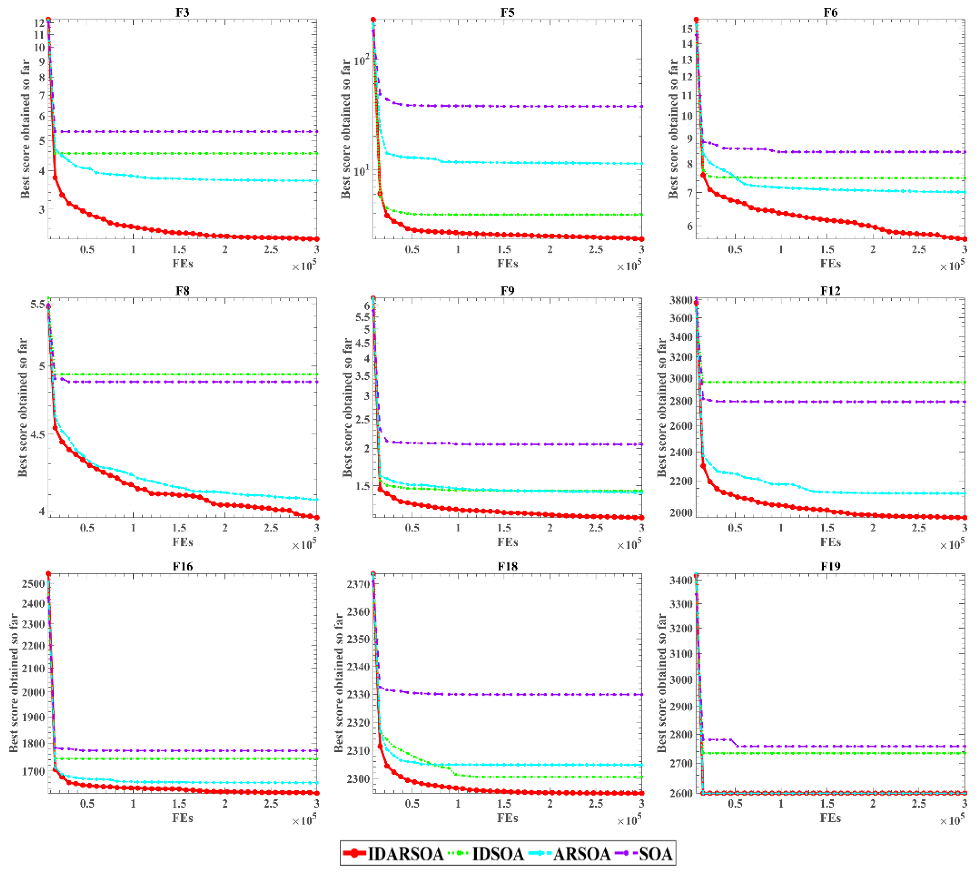
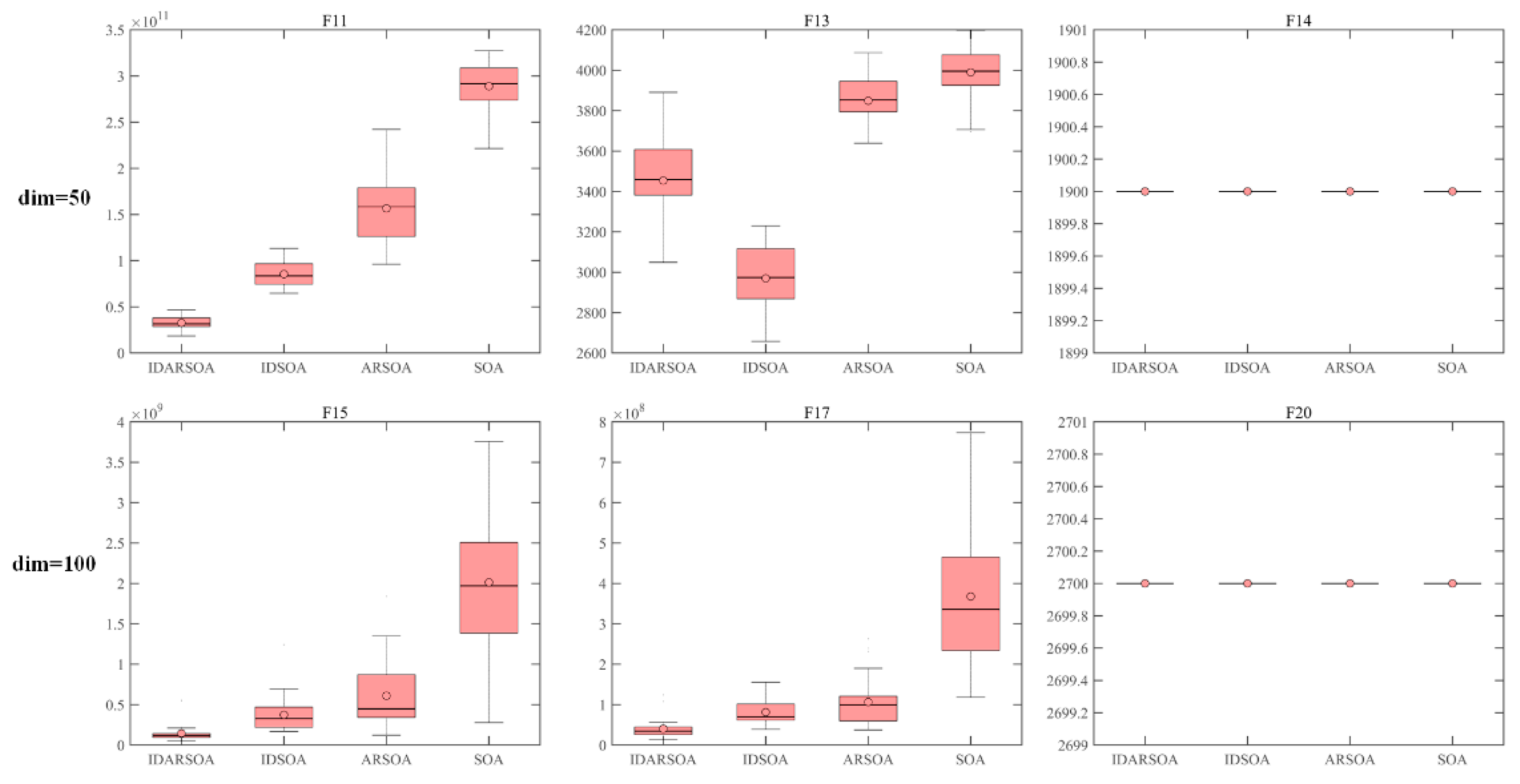
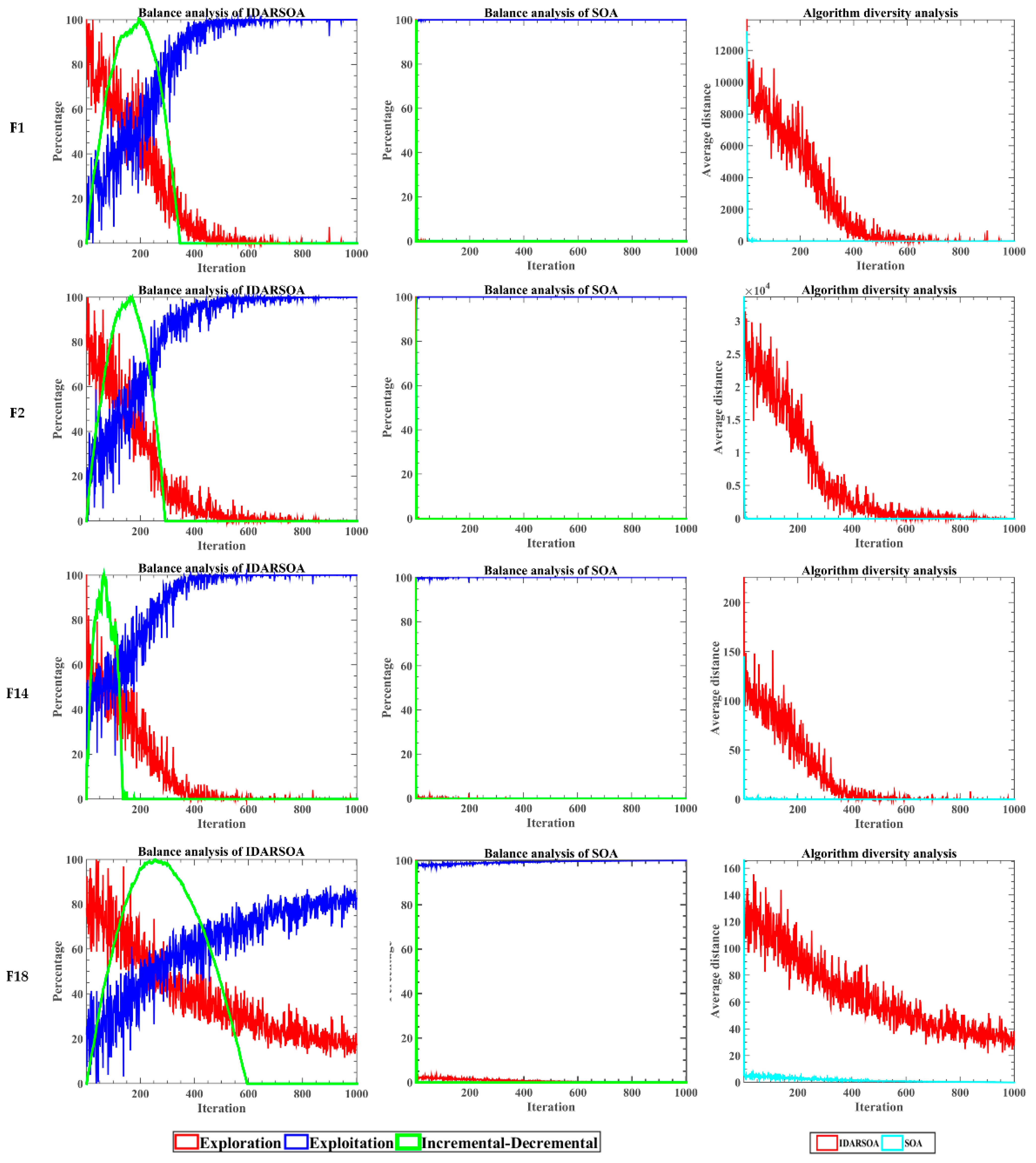
4.2. Study of the Proposed Method
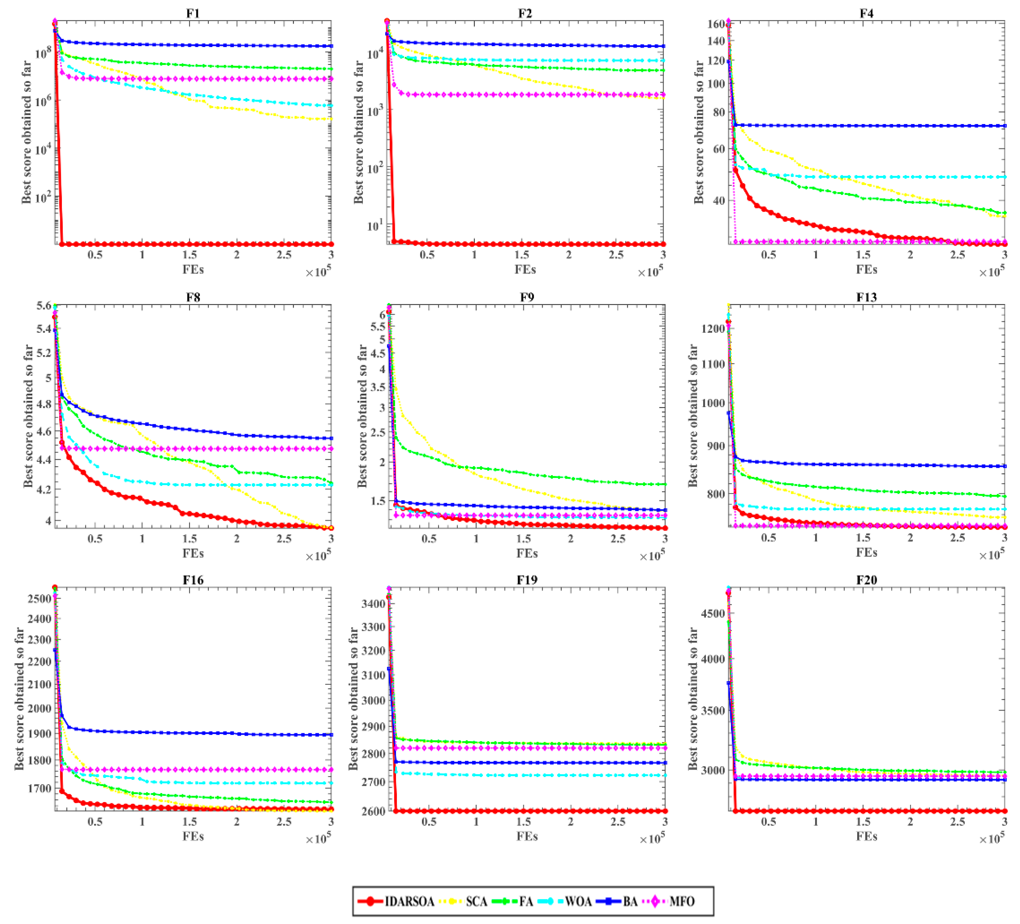
4.3. Comparative Study with Swarm Intelligence Algorithm
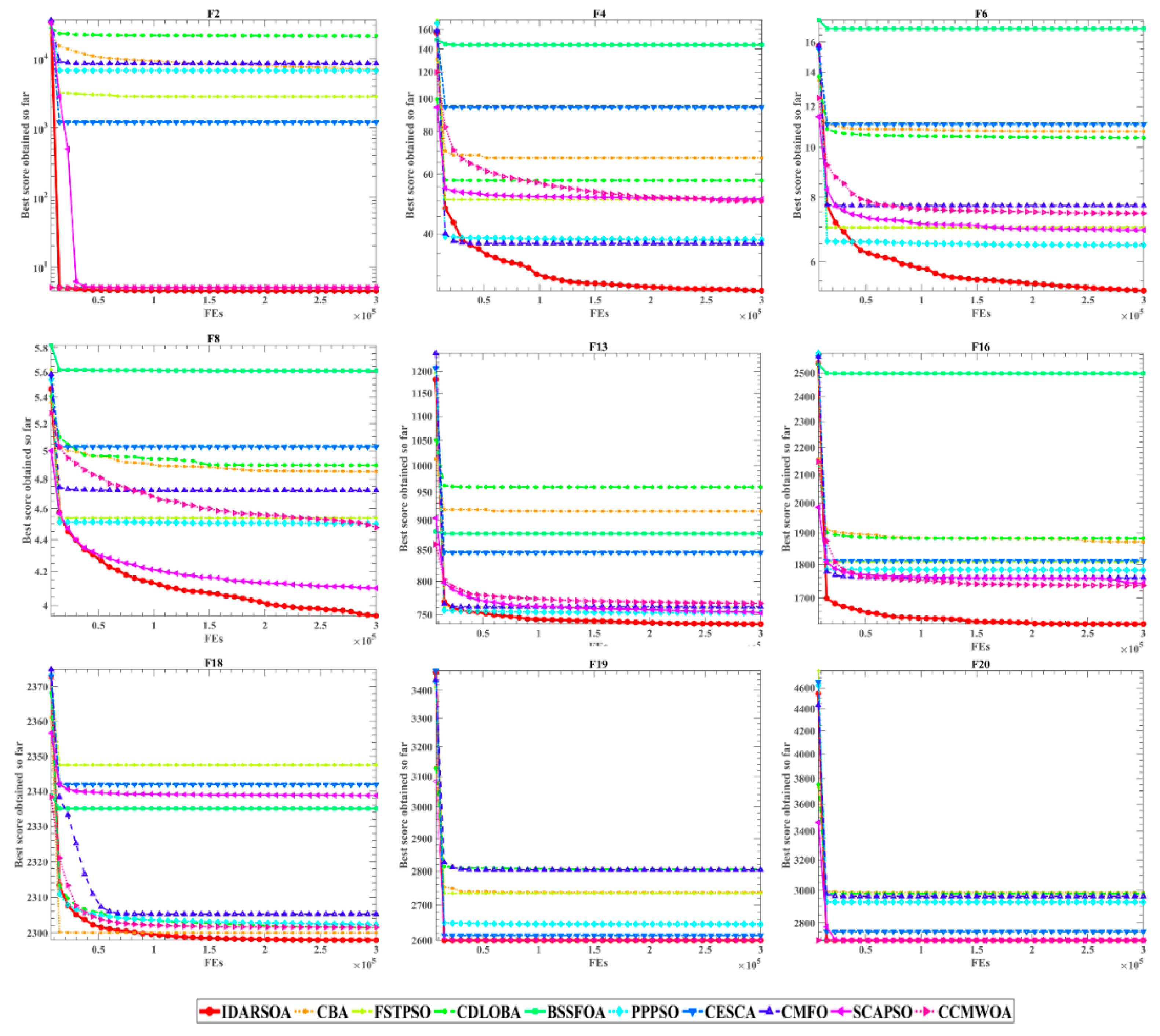
4.4. Comparative Study with Variants of Novel Intelligent Algorithms
5. Engineering Design Issues
5.1. Tension-Compression String Problem
5.2. Pressure Vessel Design Problem
5.3. I-Beam Design Problem
5.4. Speed Reducer Design Problem
5.5. Welded Beam Design Problem
5.6. Three-Bar Truss Design Problem
6. Conclusions and Future Works
Author Contributions
Funding
Institutional Review Board Statement
Informed Consent Statement
Data Availability Statement
Conflicts of Interest
Appendix A

| NO. | Functions | Dim | F (min) |
|---|---|---|---|
| CEC2019 benchmark functions | |||
| F1 | Storn’s Chebyshev Polynomial Fitting Problem | 9 | 1 |
| F2 | Inverse Hilbert Matrix Problem | 16 | 1 |
| F3 | Lennard-Joes Minimum Energy Cluster | 18 | 1 |
| F4 | Rastrigin’s Function | 10 | 1 |
| F5 | Griewangk’s Function | 10 | 1 |
| F6 | Weierstrass Function | 10 | 1 |
| F7 | Modified Schwefel’s Function | 10 | 1 |
| F8 | Expand Schaffer’s F6 function | 10 | 1 |
| F9 | Happy Cat Function | 10 | 1 |
| F10 | Ackley Function | 10 | 1 |
| CEC2020 benchmark functions | |||
| F11 | Shifted and Rotated Bent Cigar Function (CEC2017 F1) | 30 | 100 |
| F12 | Shifted and Rotated Schwefel’s Function (CEC2014 F11) | 30 | 1100 |
| F13 | Shifted and Rotated Lunacek bi-Rastrigin Function (CEC2017 F7) | 30 | 700 |
| F14 | Expanded Rosenbrock’s plus Griewangk’s Function (CEC2017 F19) | 30 | 1900 |
| F15 | Hybrid Function1 (n = 3) (CEC2014 F17) | 30 | 1700 |
| F16 | Hybrid Function2 (n = 4) (CEC2017 F16) | 30 | 1600 |
| F17 | Hybrid Function3 (n = 5) (CEC2014 F21) | 30 | 2100 |
| F18 | Composition Function1 (n = 3) (CEC2017 F22) | 30 | 2200 |
| F19 | Composition Function2 (n = 4) (CEC2017 F24) | 30 | 2400 |
| F20 | Composition Function3 (n = 5) (CEC2017 F25) | 30 | 2500 |
References
- Beni, G.; Wang, J. Swarm intelligence in cellular robotic systems. In Robots and Biological Systems: Towards a New Bionics? Springer: Cham, Switzerland, 1993; pp. 703–712. [Google Scholar]
- Mirjalili, S.; Lewis, A. The whale optimization algorithm. Adv. Eng. Softw. 2016, 95, 51–67. [Google Scholar] [CrossRef]
- Yang, Y.; Chen, H.; Heidari, A.A.; Gandomi, A.H. Hunger games search: Visions, conception, implementation, deep analysis, perspectives, and towards performance shifts. Expert Syst. Appl. 2021, 177, 114864. [Google Scholar] [CrossRef]
- Tu, J.; Chen, H.; Wang, M.; Gandomi, A.H. The Colony Predation Algorithm. J. Bionic Eng. 2021, 18, 674–710. [Google Scholar] [CrossRef]
- Li, S.; Chen, H.; Wang, M.; Heidari, A.A.; Mirjalili, S. Slime mould algorithm: A new method for stochastic optimization. Future Gener. Comput. Syst. 2020, 111, 300–323. [Google Scholar] [CrossRef]
- Ahmadianfar, I.; Asghar Heidari, A.; Gandomi, A.H.; Chu, X.; Chen, H. RUN Beyond the Metaphor: An Efficient Optimization Algorithm Based on Runge Kutta Method. Expert Syst. Appl. 2021, 181, 115079. [Google Scholar] [CrossRef]
- Piri, J.; Mohapatra, P. An analytical study of modified multi-objective Harris Hawk Optimizer towards medical data feature selection. Comput. Biol. Med. 2021, 135, 104558. [Google Scholar] [CrossRef] [PubMed]
- Chen, M.-R.; Huang, Y.-Y.; Zeng, G.-Q.; Lu, K.-D.; Yang, L.-Q. An improved bat algorithm hybridized with extremal optimization and Boltzmann selection. Expert Syst. Appl. 2021, 175, 114812. [Google Scholar] [CrossRef]
- Tang, C.; Zhou, Y.; Tang, Z.; Luo, Q. Teaching-learning-based pathfinder algorithm for function and engineering optimization problems. Appl. Intell. 2021, 51, 5040–5066. [Google Scholar] [CrossRef]
- Zhong, L.; Zhou, Y.; Luo, Q.; Zhong, K. Wind driven dragonfly algorithm for global optimization. Concurr. Comput. Pract. Exp. 2021, 33, e6054. [Google Scholar] [CrossRef]
- Salgotra, R.; Singh, U.; Singh, S.; Singh, G.; Mittal, N. Self-adaptive salp swarm algorithm for engineering optimization problems. Appl. Math. Model. 2021, 89, 188–207. [Google Scholar] [CrossRef]
- Mirjalili, S.; Gandomi, A.H.; Mirjalili, S.Z.; Saremi, S.; Faris, H.; Mirjalili, S.M. Salp Swarm Algorithm: A bio-inspired optimizer for engineering design problems. Adv. Eng. Softw. 2017, 114, 163–191. [Google Scholar] [CrossRef]
- Kapoor, S.; Zeya, I.; Singhal, C.; Nanda, S.J. A Grey Wolf Optimizer Based Automatic Clustering Algorithm for Satellite Image Segmentation. Procedia Comput. Sci. 2017, 115, 415–422. [Google Scholar] [CrossRef]
- Seyyedabbasi, A.; Kiani, F. I-GWO and Ex-GWO: Improved algorithms of the Grey Wolf Optimizer to solve global optimization problems. Eng. Comput. 2021, 37, 509–532. [Google Scholar] [CrossRef]
- Yang, Z.; Li, K.; Guo, Y.; Ma, H.; Zheng, M. Compact real-valued teaching-learning based optimization with the applications to neural network training. Knowl.-Based Syst. 2018, 159, 51–62. [Google Scholar] [CrossRef]
- Fan, C.; Hu, K.; Feng, S.; Ye, J.; Fan, E. Heronian mean operators of linguistic neutrosophic multisets and their multiple attribute decision-making methods. Int. J. Distrib. Sens. Netw. 2019, 15, 1550147719843059. [Google Scholar] [CrossRef]
- Cui, W.-H.; Ye, J. Logarithmic similarity measure of dynamic neutrosophic cubic sets and its application in medical diagnosis. Comput. Ind. 2019, 111, 198–206. [Google Scholar] [CrossRef]
- Fan, C.; Fan, E.; Hu, K. New form of single valued neutrosophic uncertain linguistic variables aggregation operators for decision-making. Cogn. Syst. Res. 2018, 52, 1045–1055. [Google Scholar] [CrossRef] [Green Version]
- Ye, J.; Cui, W. Modeling and stability analysis methods of neutrosophic transfer functions. Soft Comput. 2020, 24, 9039–9048. [Google Scholar] [CrossRef]
- Lai, X.; Zhou, Y. Analysis of multiobjective evolutionary algorithms on the biobjective traveling salesman problem (1, 2). Multimed. Tools Appl. 2020, 79, 30839–30860. [Google Scholar] [CrossRef]
- Hu, K.; Ye, J.; Fan, E.; Shen, S.; Huang, L.; Pi, J. A novel object tracking algorithm by fusing color and depth information based on single valued neutrosophic cross-entropy. J. Intell. Fuzzy Syst. 2017, 32, 1775–1786. [Google Scholar] [CrossRef] [Green Version]
- Hu, K.; He, W.; Ye, J.; Zhao, L.; Peng, H.; Pi, J. Online Visual Tracking of Weighted Multiple Instance Learning via Neutrosophic Similarity-Based Objectness Estimation. Symmetry 2019, 11, 832. [Google Scholar] [CrossRef] [Green Version]
- Zhao, D.; Liu, L.; Yu, F.; Heidari, A.A.; Wang, M.; Liang, G.; Muhammad, K.; Chen, H. Chaotic random spare ant colony optimization for multi-threshold image segmentation of 2D Kapur entropy. Knowl.-Based Syst. 2020, 216, 106510. [Google Scholar] [CrossRef]
- Zhao, D.; Liu, L.; Yu, F.; Asghar Heidari, A.; Wang, M.; Oliva, D.; Muhammad, K.; Chen, H. Ant Colony Optimization with Horizontal and Vertical Crossover Search: Fundamental Visions for Multi-threshold Image Segmentation. Expert Syst. Appl. 2020, 167, 114122. [Google Scholar] [CrossRef]
- Zhang, Y.; Liu, R.; Wang, X.; Chen, H.; Li, C. Boosted binary Harris hawks optimizer and feature selection. Eng. Comput. 2020, 37, 3741–3770. [Google Scholar] [CrossRef]
- Hu, J.; Chen, H.; Heidari, A.A.; Wang, M.; Zhang, X.; Chen, Y.; Pan, Z. Orthogonal learning covariance matrix for defects of grey wolf optimizer: Insights, balance, diversity, and feature selection. Knowl.-Based Syst. 2021, 213, 106684. [Google Scholar] [CrossRef]
- Zhang, X.; Xu, Y.; Yu, C.; Heidari, A.A.; Li, S.; Chen, H.; Li, C. Gaussian mutational chaotic fruit fly-built optimization and feature selection. Expert Syst. Appl. 2020, 141, 112976. [Google Scholar] [CrossRef]
- Li, Q.; Chen, H.; Huang, H.; Zhao, X.; Cai, Z.; Tong, C.; Liu, W.; Tian, X. An Enhanced Grey Wolf Optimization Based Feature Selection Wrapped Kernel Extreme Learning Machine for Medical Diagnosis. Comput. Math. Methods Med. 2017, 2017, 9512741. [Google Scholar] [CrossRef] [PubMed]
- Liu, T.; Hu, L.; Ma, C.; Wang, Z.-Y.; Chen, H.-L. A fast approach for detection of erythemato-squamous diseases based on extreme learning machine with maximum relevance minimum redundancy feature selection. Int. J. Syst. Sci. 2015, 46, 919–931. [Google Scholar] [CrossRef]
- Gupta, S.; Deep, K.; Heidari, A.A.; Moayedi, H.; Chen, H. Harmonized salp chain-built optimization. Eng. Comput. 2019, 37, 1049–1079. [Google Scholar] [CrossRef]
- Ba, A.F.; Huang, H.; Wang, M.; Ye, X.; Gu, Z.; Chen, H.; Cai, X. Levy-based antlion-inspired optimizers with orthogonal learning scheme. Eng. Comput. 2020, 1–22. [Google Scholar] [CrossRef]
- Zhang, H.; Cai, Z.; Ye, X.; Wang, M.; Kuang, F.; Chen, H.; Li, C.; Li, Y. A multi-strategy enhanced salp swarm algorithm for global optimization. Eng. Comput. 2020, 1–27. [Google Scholar] [CrossRef]
- Liang, X.; Cai, Z.; Wang, M.; Zhao, X.; Chen, H.; Li, C. Chaotic oppositional sine–cosine method for solving global optimization problems. Eng. Comput. 2020, 1–17. [Google Scholar] [CrossRef]
- Pang, J.; Zhou, H.; Tsai, Y.-C.; Chou, F.-D. A scatter simulated annealing algorithm for the bi-objective scheduling problem for the wet station of semiconductor manufacturing. Comput. Ind. Eng. 2018, 123, 54–66. [Google Scholar] [CrossRef]
- Zhou, H.; Pang, J.; Chen, P.-K.; Chou, F.-D. A modified particle swarm optimization algorithm for a batch-processing machine scheduling problem with arbitrary release times and non-identical job sizes. Comput. Ind. Eng. 2018, 123, 67–81. [Google Scholar] [CrossRef]
- Hu, L.; Li, H.; Cai, Z.; Lin, F.; Hong, G.; Chen, H.; Lu, Z. A new machine-learning method to prognosticate paraquat poisoned patients by combining coagulation, liver, and kidney indices. PLoS ONE 2017, 12, e0186427. [Google Scholar] [CrossRef] [PubMed] [Green Version]
- Li, C.; Hou, L.; Sharma, B.Y.; Li, H.; Chen, C.; Li, Y.; Zhao, X.; Huang, H.; Cai, Z.; Chen, H. Developing a new intelligent system for the diagnosis of tuberculous pleural effusion. Comput. Methods Programs Biomed. 2018, 153, 211–225. [Google Scholar] [CrossRef]
- Zhao, X.; Zhang, X.; Cai, Z.; Tian, X.; Wang, X.; Huang, Y.; Chen, H.; Hu, L. Chaos enhanced grey wolf optimization wrapped ELM for diagnosis of paraquat-poisoned patients. Comput. Biol. Chem. 2019, 78, 481–490. [Google Scholar] [CrossRef]
- Huang, H.; Zhou, S.; Jiang, J.; Chen, H.; Li, Y.; Li, C. A new fruit fly optimization algorithm enhanced support vector machine for diagnosis of breast cancer based on high-level features. BMC Bioinform. 2019, 20, 290. [Google Scholar] [CrossRef] [Green Version]
- Zhang, Y.; Liu, R.; Heidari, A.A.; Wang, X.; Chen, Y.; Wang, M.; Chen, H. Towards augmented kernel extreme learning models for bankruptcy prediction: Algorithmic behavior and comprehensive analysis. Neurocomputing 2020, 430, 185–212. [Google Scholar] [CrossRef]
- Yu, C.; Chen, M.; Cheng, K.; Zhao, X.; Ma, C.; Kuang, F.; Chen, H. SGOA: Annealing-behaved grasshopper optimizer for global tasks. Eng. Comput. 2021. [Google Scholar] [CrossRef]
- Cai, Z.; Gu, J.; Luo, J.; Zhang, Q.; Chen, H.; Pan, Z.; Li, Y.; Li, C. Evolving an optimal kernel extreme learning machine by using an enhanced grey wolf optimization strategy. Expert Syst. Appl. 2019, 138, 112814. [Google Scholar] [CrossRef]
- Heidari, A.A.; Abbaspour, R.A.; Chen, H. Efficient boosted grey wolf optimizers for global search and kernel extreme learning machine training. Appl. Soft Comput. 2019, 81, 105521. [Google Scholar] [CrossRef]
- Shen, L.; Chen, H.; Yu, Z.; Kang, W.; Zhang, B.; Li, H.; Yang, B.; Liu, D. Evolving support vector machines using fruit fly optimization for medical data classification. Knowl.-Based Syst. 2016, 96, 61–75. [Google Scholar] [CrossRef]
- Wang, M.; Chen, H.; Yang, B.; Zhao, X.; Hu, L.; Cai, Z.; Huang, H.; Tong, C. Toward an optimal kernel extreme learning machine using a chaotic moth-flame optimization strategy with applications in medical diagnoses. Neurocomputing 2017, 267, 69–84. [Google Scholar] [CrossRef]
- Wang, M.; Chen, H. Chaotic multi-swarm whale optimizer boosted support vector machine for medical diagnosis. Appl. Soft Comput. 2020, 88, 105946. [Google Scholar] [CrossRef]
- Deng, W.; Xu, J.; Zhao, H.; Song, Y. A Novel Gate Resource Allocation Method Using Improved PSO-Based QEA. IEEE Trans. Intell. Transp. Syst. 2020. [Google Scholar] [CrossRef]
- Deng, W.; Xu, J.; Song, Y.; Zhao, H. An Effective Improved Co-evolution Ant Colony Optimization Algorithm with Multi-Strategies and Its Application. Int. J. Bio-Inspired Comput. 2020, 16, 158–170. [Google Scholar] [CrossRef]
- Chen, Z.-G.; Zhan, Z.-H.; Lin, Y.; Gong, Y.-J.; Gu, T.-L.; Zhao, F.; Yuan, H.-Q.; Chen, X.; Li, Q.; Zhang, J. Multiobjective cloud workflow scheduling: A multiple populations ant colony system approach. IEEE Trans. Cybern. 2018, 49, 2912–2926. [Google Scholar] [CrossRef]
- Wang, Z.-J.; Zhan, Z.-H.; Yu, W.-J.; Lin, Y.; Zhang, J.; Gu, T.-L.; Zhang, J. Dynamic group learning distributed particle swarm optimization for large-scale optimization and its application in cloud workflow scheduling. IEEE Trans. Cybern. 2019, 50, 2715–2729. [Google Scholar] [CrossRef]
- Deng, W.; Liu, H.; Xu, J.; Zhao, H.; Song, Y. An improved quantum-inspired differential evolution algorithm for deep belief network. IEEE Trans. Instrum. Meas. 2020, 69, 7319–7327. [Google Scholar] [CrossRef]
- Zhao, H.; Liu, H.; Xu, J.; Deng, W. Performance prediction using high-order differential mathematical morphology gradient spectrum entropy and extreme learning machine. IEEE Trans. Instrum. Meas. 2019, 69, 4165–4172. [Google Scholar] [CrossRef]
- Liu, X.-F.; Zhan, Z.-H.; Zhang, J. Resource-Aware Distributed Differential Evolution for Training Expensive Neural-Network-Based Controller in Power Electronic Circuit. IEEE Trans. Neural Netw. Learn. Syst. 2021. [Google Scholar] [CrossRef]
- Zhan, Z.-H.; Liu, X.-F.; Zhang, H.; Yu, Z.; Weng, J.; Li, Y.; Gu, T.; Zhang, J. Cloudde: A heterogeneous differential evolution algorithm and its distributed cloud version. IEEE Trans. Parallel Distrib. Syst. 2016, 28, 704–716. [Google Scholar] [CrossRef]
- Zhao, X.; Li, D.; Yang, B.; Ma, C.; Zhu, Y.; Chen, H. Feature selection based on improved ant colony optimization for online detection of foreign fiber in cotton. Appl. Soft Comput. 2014, 24, 585–596. [Google Scholar] [CrossRef]
- Zhao, X.; Li, D.; Yang, B.; Chen, H.; Yang, X.; Yu, C.; Liu, S. A two-stage feature selection method with its application. Comput. Electr. Eng. 2015, 47, 114–125. [Google Scholar] [CrossRef]
- Liang, D.; Zhan, Z.-H.; Zhang, Y.; Zhang, J. An efficient ant colony system approach for new energy vehicle dispatch problem. IEEE Trans. Intell. Transp. Syst. 2019, 21, 4784–4797. [Google Scholar] [CrossRef]
- Ridha, H.M.; Heidari, A.A.; Wang, M.; Chen, H. Boosted mutation-based Harris hawks optimizer for parameters identification of single-diode solar cell models. Energy Convers. Manag. 2020, 209, 112660. [Google Scholar] [CrossRef]
- Dhiman, G.; Kumar, V. Seagull optimization algorithm: Theory and its applications for large-scale industrial engineering problems. Knowl.-Based Syst. 2019, 165, 169–196. [Google Scholar] [CrossRef]
- Lei, G.; Song, H.; Rodriguez, D. Power generation cost minimization of the grid-connected hybrid renewable energy system through optimal sizing using the modified seagull optimization technique. Energy Rep. 2020, 6, 3365–3376. [Google Scholar] [CrossRef]
- Cao, Y.; Li, Y.; Zhang, G.; Jermsittiparsert, K.; Razmjooy, N. Experimental modeling of PEM fuel cells using a new improved seagull optimization algorithm. Energy Rep. 2019, 5, 1616–1625. [Google Scholar] [CrossRef]
- Dhiman, G.; Singh, K.K.; Soni, M.; Nagar, A.; Dehghani, M.; Slowik, A.; Kaur, A.; Sharma, A.; Houssein, E.H.; Cengiz, K. MOSOA: A new multi-objective seagull optimization algorithm. Expert Syst. Appl. 2021, 167, 114150. [Google Scholar] [CrossRef]
- Riget, J.; Vesterstrøm, J.S. A diversity-guided particle swarm optimizer-the ARPSO. Dept. Comput. Sci. Univ. of Aarhus Aarhus Denmark Tech. Rep. 2002, 2, 2002. [Google Scholar]
- Pant, M.; Radha, T.; Singh, V.P. A simple diversity guided particle swarm optimization. In Proceedings of the 2007 IEEE Congress on Evolutionary Computation, Singapore, 25–28 September 2007; pp. 3294–3299. [Google Scholar]
- Mohamed, N.; Bilel, N.; Alsagri, A.S. A multi-objective methodology for multi-criteria engineering design. Appl. Soft Comput. 2020, 91, 106204. [Google Scholar] [CrossRef]
- Price, K.; Awad, N.; Ali, M.; Suganthan, P. Problem definitions and evaluation criteria for the 100-digit challenge special session and competition on single objective numerical optimization. In Technical Report; Nanyang Technological University: Singapore, 2018. [Google Scholar]
- Ahmed, A.M.; Rashid, T.A.; Saeed, S.A.M. Cat swarm optimization algorithm: A survey and performance evaluation. Comput. Intell. Neurosci. 2020, 2020, 4854895. [Google Scholar] [CrossRef]
- Rahman, C.M.; Rashid, T.A. A new evolutionary algorithm: Learner performance based behavior algorithm. Egypt. Inform. J. 2021, 22, 213–223. [Google Scholar] [CrossRef]
- Abdullah, J.M.; Ahmed, T. Fitness dependent optimizer: Inspired by the bee swarming reproductive process. IEEE Access 2019, 7, 43473–43486. [Google Scholar] [CrossRef]
- Rahman, C.M.; Rashid, T.A. Dragonfly algorithm and its applications in applied science survey. Comput. Intell. Neurosci. 2019, 2019, 9293617. [Google Scholar] [CrossRef]
- Li, Z.; Tam, V. A novel meta-heuristic optimization algorithm inspired by the spread of viruses. arXiv 2020, arXiv:2006.06282. [Google Scholar]
- Mirjalili, S. SCA: A sine cosine algorithm for solving optimization problems. Knowl.-Based Syst. 2016, 96, 120–133. [Google Scholar] [CrossRef]
- Yang, X.-S. Firefly algorithms for multimodal optimization. In International Symposium on Stochastic Algorithms; Springer: Berlin/Heidelberg, Germany, 2009; pp. 169–178. [Google Scholar]
- Yang, X.-S. A new metaheuristic bat-inspired algorithm. In Nature Inspired Cooperative Strategies for Optimization (NICSO 2010); Springer: Berlin/Heidelberg, Germany, 2010; pp. 65–74. [Google Scholar]
- Mirjalili, S. Moth-flame optimization algorithm: A novel nature-inspired heuristic paradigm. Knowl.-Based Syst. 2015, 89, 228–249. [Google Scholar] [CrossRef]
- Adarsh, B.; Raghunathan, T.; Jayabarathi, T.; Yang, X.-S. Economic dispatch using chaotic bat algorithm. Energy 2016, 96, 666–675. [Google Scholar] [CrossRef]
- Nobile, M.S.; Cazzaniga, P.; Besozzi, D.; Colombo, R.; Mauri, G.; Pasi, G. Fuzzy Self-Tuning PSO: A settings-free algorithm for global optimization. Swarm Evol. Comput. 2018, 39, 70–85. [Google Scholar] [CrossRef]
- Yong, J.; He, F.; Li, H.; Zhou, W. A novel bat algorithm based on collaborative and dynamic learning of opposite population. In Proceedings of the 2018 IEEE 22nd International Conference on Computer Supported Cooperative Work in Design (CSCWD), Nanjing, China, 9–11 May 2018; pp. 541–546. [Google Scholar]
- Zhang, H.; Yuan, M.; Liang, Y.; Liao, Q. A novel particle swarm optimization based on prey–predator relationship. Appl. Soft Comput. 2018, 68, 202–218. [Google Scholar] [CrossRef]
- Lin, A.; Wu, Q.; Heidari, A.A.; Xu, Y.; Chen, H.; Geng, W.; Li, C. Predicting intentions of students for master programs using a chaos-induced sine cosine-based fuzzy K-nearest neighbor classifier. IEEE Access 2019, 7, 67235–67248. [Google Scholar] [CrossRef]
- Hongwei, L.; Jianyong, L.; Liang, C.; Jingbo, B.; Yangyang, S.; Kai, L.J. Chaos-enhanced moth-flame optimization algorithm for global optimization. J. Syst. Eng. Electron. 2019, 30, 1144–1159. [Google Scholar]
- Nenavath, H.; Jatoth, R.K.; Das, S. A synergy of the sine-cosine algorithm and particle swarm optimizer for improved global optimization and object tracking. Swarm Evol. Comput. 2018, 43, 1–30. [Google Scholar] [CrossRef]
- Luo, J.; Chen, H.; Heidari, A.A.; Xu, Y.; Zhang, Q.; Li, C. Multi-strategy boosted mutative whale-inspired optimization approaches. Appl. Math. Model. 2019, 73, 109–123. [Google Scholar] [CrossRef]
- Fan, Y.; Wang, P.; Mafarja, M.; Wang, M.; Zhao, X.; Chen, H. A bioinformatic variant fruit fly optimizer for tackling optimization problems. Knowl.-Based Syst. 2021, 213, 106704. [Google Scholar] [CrossRef]
- Hu, Z.; Wang, J.; Zhang, C.; Luo, Z.; Luo, X.; Xiao, L.; Shi, J. Uncertainty Modeling for Multi center Autism Spectrum Disorder Classification Using Takagi-Sugeno-Kang Fuzzy Systems. IEEE Trans. Cogn. Dev. Syst. 2021. [Google Scholar] [CrossRef]
- Chen, C.; Wu, Q.; Li, Z.; Xiao, L.; Hu, Z.Y. Diagnosis of Alzheimer’s disease based on Deeply-Fused Nets. Comb. Chem. High Throughput Screen. 2020, 24, 781–789. [Google Scholar] [CrossRef]
- Fei, X.; Wang, J.; Ying, S.; Hu, Z.; Shi, J. Projective parameter transfer based sparse multiple empirical kernel learning Machine for diagnosis of brain disease. Neurocomputing 2020, 413, 271–283. [Google Scholar] [CrossRef]
- Saber, A.; Sakr, M.; Abo-Seida, O.M.; Keshk, A.; Chen, H. A Novel Deep-Learning Model for Automatic Detection and Classification of Breast Cancer Using the Transfer-Learning Technique. IEEE Access 2021, 9, 71194–71209. [Google Scholar] [CrossRef]
- Cao, X.Y.; Wang, J.X.; Wang, J.H.; Zeng, B. A Risk-Averse Conic Model for Networked Microgrids Planning With Reconfiguration and Reorganizations. IEEE Trans. Smart Grid 2020, 11, 696–709. [Google Scholar] [CrossRef]
- Cao, X.; Cao, T.; Gao, F.; Guan, X. Risk-Averse Storage Planning for Improving RES Hosting Capacity under Uncertain Siting Choice. IEEE Trans. Sustain. Energy 2021. [Google Scholar] [CrossRef]
- Pei, H.; Yang, B.; Liu, J.; Chang, K. Active Surveillance via Group Sparse Bayesian Learning. IEEE Trans. Pattern Anal. Mach. Intell. 2020. [Google Scholar] [CrossRef] [PubMed]
- Qiu, S.; Hao, Z.; Wang, Z.; Liu, L.; Liu, J.; Zhao, H.; Fortino, G. Sensor Combination Selection Strategy for Kayak Cycle Phase Segmentation Based on Body Sensor Networks. IEEE Internet Things J. 2021. [Google Scholar] [CrossRef]
- Wu, Z.; Li, G.; Shen, S.; Cui, Z.; Lian, X.; Xu, G. Constructing dummy query sequences to protect location privacy and query privacy in location-based services. World Wide Web 2021, 24, 25–49. [Google Scholar] [CrossRef]
- Wu, Z.; Wang, R.; Li, Q.; Lian, X.; Xu, G. A location privacy-preserving system based on query range cover-up for location-based services. IEEE Trans. Veh. Technol. 2020, 69, 5244–5254. [Google Scholar] [CrossRef]
- Zhang, X.; Wang, T.; Wang, J.; Tang, G.; Zhao, L. Pyramid channel-based feature attention network for image dehazing. Comput. Vis. Image Underst. 2020, 197, 103003. [Google Scholar] [CrossRef]
- Wu, Z.; Li, R.; Xie, J.; Zhou, Z.; Guo, J.; Xu, X. A user sensitive subject protection approach for book search service. J. Assoc. Inf. Sci. Technol. 2020, 71, 183–195. [Google Scholar] [CrossRef]
- Wu, Z.; Shen, S.; Lian, X.; Su, X.; Chen, E. A dummy-based user privacy protection approach for text information retrieval. Knowl.-Based Syst. 2020, 195, 105679. [Google Scholar] [CrossRef]
- Wu, Z.; Shen, S.; Zhou, H.; Li, H.; Lu, C.; Zou, D. An effective approach for the protection of user commodity viewing privacy in e-commerce website. Knowl.-Based Syst. 2021, 220, 106952. [Google Scholar] [CrossRef]
- Qiu, S.; Zhao, H.; Jiang, N.; Wu, D.; Song, G.; Zhao, H.; Wang, Z. Sensor network oriented human motion capture via wearable intelligent system. Int. J. Intell. Syst. 2022, 137, 1646–1673. [Google Scholar] [CrossRef]
- Zhang, X.; Jiang, R.; Wang, T.; Wang, J. Recursive Neural Network for Video Deblurring. IEEE Trans. Circuits Syst. Video Technol. 2021, 31, 3025–3036. [Google Scholar] [CrossRef]
- Mahdavi, M.; Fesanghary, M.; Damangir, E. An improved harmony search algorithm for solving optimization problems. Appl. Math. Comput. 2007, 188, 1567–1579. [Google Scholar] [CrossRef]
- Kennedy, J.; Eberhart, R. Particle swarm optimization. In Proceedings of the ICNN’95-International Conference on Neural Networks, Perth, Australia, 27 November–1 December 1995; pp. 1942–1948. [Google Scholar]
- Kaveh, A.; Khayatazad, M. A new meta-heuristic method: Ray optimization. Comput. Struct. 2012, 112, 283–294. [Google Scholar] [CrossRef]
- Mezura-Montes, E.; Coello, C.A.C. An empirical study about the usefulness of evolution strategies to solve constrained optimization problems. Int. J. Gen. Syst. 2008, 37, 443–473. [Google Scholar] [CrossRef]
- Rashedi, E.; Nezamabadi-Pour, H.; Saryazdi, S. GSA: A Gravitational Search Algorithm. Inf. Sci. 2009, 179, 2232–2248. [Google Scholar] [CrossRef]
- Coello, C.A.C. Use of a self-adaptive penalty approach for engineering optimization problems. Comput. Ind. 2000, 41, 113–127. [Google Scholar] [CrossRef]
- Kannan, B.; Kramer, S.N. An augmented Lagrange multiplier based method for mixed integer discrete continuous optimization and its applications to mechanical design. In International Design Engineering Technical Conferences and Computers and Information in Engineering Conference; American Society of Mechanical Engineers: New York, NY, USA, 1994; pp. 103–112. [Google Scholar]
- Sandgren, E. Nonlinear Integer and Discrete Programming in Mechanical Design Optimization. J. Mech. Des. 1990, 112, 223–229. [Google Scholar] [CrossRef]
- Cheng, M.-Y.; Prayogo, D. Symbiotic organisms search: A new metaheuristic optimization algorithm. Comput. Struct. 2014, 139, 98–112. [Google Scholar] [CrossRef]
- Gandomi, A.H.; Yang, X.-S.; Alavi, A.H. Cuckoo search algorithm: A metaheuristic approach to solve structural optimization problems. Eng. Comput. 2013, 29, 17–35. [Google Scholar] [CrossRef]
- Wang, G.; Heidari, A.A.; Wang, M.; Kuang, F.; Zhu, W.; Chen, H. Chaotic arc adaptive grasshopper optimization. IEEE Access 2021, 9, 17672–17706. [Google Scholar] [CrossRef]
- Wang, G.G. Adaptive response surface method using inherited latin hypercube design points. J. Mech. Des. 2003, 125, 210–220. [Google Scholar] [CrossRef]
- Kamboj, V.K.; Nandi, A.; Bhadoria, A.; Sehgal, S. An intensify Harris Hawks optimizer for numerical and engineering optimization problems. Appl. Soft Comput. 2020, 89, 106018. [Google Scholar] [CrossRef]
- Faramarzi, A.; Heidarinejad, M.; Stephens, B.; Mirjalili, S. Equilibrium optimizer: A novel optimization algorithm. Knowl.-Based Syst. 2020, 191, 105190. [Google Scholar] [CrossRef]
- Lee, K.S.; Geem, Z.W. A new meta-heuristic algorithm for continuous engineering optimization: Harmony search theory and practice. Comput. Methods Appl. Mech. Eng. 2005, 194, 3902–3933. [Google Scholar] [CrossRef]
- Hedar, A.-R.; Fukushima, M. Derivative-free filter simulated annealing method for constrained continuous global optimization. J. Glob. Optim. 2006, 35, 521–549. [Google Scholar] [CrossRef]
- Ray, T.; Liew, K.-M. Society and civilization: An optimization algorithm based on the simulation of social behavior. IEEE Trans. Evol. Comput. 2003, 7, 386–396. [Google Scholar] [CrossRef]
- Akhtar, S.; Tai, K.; Ray, T. A socio-behavioural simulation model for engineering design optimization. Eng. Optim. 2002, 34, 341–354. [Google Scholar] [CrossRef]
- Mirjalili, S.; Mirjalili, S.M.; Lewis, A. Grey wolf optimizer. Adv. Eng. Softw. 2014, 69, 46–61. [Google Scholar] [CrossRef] [Green Version]
- Nenavath, H.; Jatoth, R.K. Hybridizing sine cosine algorithm with differential evolution for global optimization and object tracking. Appl. Soft Comput. 2018, 62, 1019–1043. [Google Scholar] [CrossRef]
- Chen, W.-N.; Zhang, J.; Lin, Y.; Chen, N.; Zhan, Z.-H.; Chung, H.S.-H.; Li, Y.; Shi, Y.-H. Particle swarm optimization with an aging leader and challengers. IEEE Trans. Evol. Comput. 2012, 17, 241–258. [Google Scholar] [CrossRef]
- Kumar, A.; Das, S.; Zelinka, I. A self-adaptive spherical search algorithm for real-world constrained optimization problems. In Proceedings of the 2020 Genetic and Evolutionary Computation Conference Companion, Cancún, Mexico, 8–12 July 2020; pp. 13–14. [Google Scholar]
- Gurrola-Ramos, J.; Hernàndez-Aguirre, A.; Dalmau-Cedeño, O. COLSHADE for real-world single-objective constrained optimization problems. In Proceedings of the 2020 IEEE Congress on Evolutionary Computation (CEC), Glasgow, UK, 19–24 July 2020; pp. 1–8. [Google Scholar]
- Kumar, A.; Das, S.; Zelinka, I. A modified covariance matrix adaptation evolution strategy for real-world constrained optimization problems. In Proceedings of the 2020 Genetic and Evolutionary Computation Conference Companion, Cancún, Mexico, 8–12 July 2020; pp. 11–12. [Google Scholar]
- Li, J.; Xiao, D.-D.; Zhang, T.; Liu, C.; Li, Y.-X.; Wang, G.-G. Multi-swarm cuckoo search algorithm with Q-learning model. Comput. J. 2020, 64, 108–131. [Google Scholar] [CrossRef]
- Nan, X.; Bao, L.; Zhao, X.; Zhao, X.; Sangaiah, A.K.; Wang, G.-G.; Ma, Z. EPuL: An enhanced positive-unlabeled learning algorithm for the prediction of pupylation sites. Molecules 2017, 22, 1463. [Google Scholar] [CrossRef] [PubMed] [Green Version]
- Liu, D.; Fan, Z.; Fu, Q.; Li, M.; Faiz, M.A.; Ali, S.; Li, T.; Zhang, L.; Khan, M.I. Random forest regression evaluation model of regional flood disaster resilience based on the whale optimization algorithm. J. Clean. Prod. 2020, 250, 119468. [Google Scholar] [CrossRef]
- Gu, Z.-M.; Wang, G.-G. Improving NSGA-III algorithms with information feedback models for large-scale many-objective optimization. Future Gener. Comput. Syst. 2020, 107, 49–69. [Google Scholar] [CrossRef]
- Yi, J.-H.; Deb, S.; Dong, J.; Alavi, A.H.; Wang, G.-G. An improved NSGA-III Algorithm with adaptive mutation operator for big data optimization problems. Future Gener. Comput. Syst. 2018, 88, 571–585. [Google Scholar] [CrossRef]
- Wang, G.-G.; Cai, X.; Cui, Z.; Min, G.; Chen, J. High performance computing for cyber physical social systems by using evolutionary multi-objective optimization algorithm. IEEE Trans. Emerg. Top. Comput. 2020, 8, 20–30. [Google Scholar] [CrossRef]
- Sun, J.; Miao, Z.; Gong, D.; Zeng, X.-J.; Li, J.; Wang, G.-G. Interval multi-objective optimization with memetic algorithms. IEEE Trans. Cybern. 2020, 50, 3444–3457. [Google Scholar] [CrossRef]


| F1 | F2 | F3 | ||||
| AVG | STD | AVG | STD | AVG | STD | |
| IDARSOAfc1 | 1.000000 × 100 | 5.758899 × 10⁻¹⁴ | 4.952258 × 100 | 1.817900 × 10⁻¹ | 2.433492 × 100 | 1.186997 × 100 |
| IDARSOAfc2 | 1.000000 × 100 | 2.667535 × 10⁻¹³ | 4.416804 × 100 | 2.696345 × 10⁻¹ | 2.125574 × 100 | 9.741309 × 10⁻¹ |
| IDARSOAfc3 | 1.000000 × 100 | 1.427971 × 10⁻¹² | 4.620769 × 100 | 3.408565 × 10⁻¹ | 2.422004 × 100 | 1.022597 × 100 |
| IDARSOAfc5 | 1.000000 × 100 | 7.603133 × 10⁻¹³ | 4.468247 × 100 | 2.786393 × 10⁻¹ | 3.079520 × 100 | 1.460601 × 100 |
| IDARSOAfc7 | 1.000000 × 100 | 3.477511 × 10⁻¹⁴ | 4.630774 × 100 | 3.173943 × 10⁻¹ | 4.326896 × 100 | 1.815038 × 100 |
| IDARSOAfc9 | 1.000000 × 100 | 2.433234 × 10⁻¹¹ | 4.729463 × 100 | 3.398487 × 10⁻¹ | 4.073180 × 100 | 1.644750 × 100 |
| F4 | F5 | F6 | ||||
| AVG | STD | AVG | STD | AVG | STD | |
| IDARSOAfc1 | 3.688039 × 101 | 1.373013 × 101 | 5.821549 × 100 | 9.047358 × 100 | 5.491320 × 100 | 1.275813 × 100 |
| IDARSOAfc2 | 2.463451 × 101 | 1.139996 × 101 | 2.194699 × 100 | 6.875180 × 10⁻¹ | 5.664204 × 100 | 1.692936 × 100 |
| IDARSOAfc3 | 2.239873 × 101 | 8.125202 × 100 | 1.998788 × 100 | 3.113314 × 10⁻¹ | 4.818130 × 100 | 1.701835 × 100 |
| IDARSOAfc5 | 2.424563 × 101 | 6.106529 × 100 | 2.061292 × 100 | 4.047150 × 10⁻¹ | 5.185845 × 100 | 1.352847 × 100 |
| IDARSOAfc7 | 2.731944 × 101 | 1.041899 × 100 | 2.108973 × 100 | 6.882413 × 10⁻¹ | 5.632649 × 100 | 1.915015 × 100 |
| IDARSOAfc9 | 2.859710 × 101 | 1.035596 × 101 | 2.131835 × 100 | 6.668301 × 10⁻¹ | 5.873998 × 100 | 2.092584 × 100 |
| F7 | F8 | F9 | ||||
| AVG | STD | AVG | STD | AVG | STD | |
| IDARSOAfc1 | 1.263735 × 10³ | 3.365559 × 10² | 4.074083 × 100 | 4.138044 × 10⁻¹ | 1.212927 × 100 | 7.951421 × 10⁻² |
| IDARSOAfc2 | 1.406561 × 10³ | 4.167857 × 10² | 3.953226 × 100 | 3.750406 × 10⁻¹ | 1.181665 × 100 | 7.032048 × 10⁻² |
| IDARSOAfc3 | 1.509095 × 10³ | 3.868018 × 10² | 3.920128 × 100 | 4.127622 × 10⁻¹ | 1.185820 × 100 | 8.267084 × 10⁻² |
| IDARSOAfc5 | 1.468453 × 10³ | 5.192703 × 10² | 4.002200 × 100 | 3.019612 × 10⁻¹ | 1.224425 × 100 | 7.752889 × 10⁻² |
| IDARSOAfc7 | 1.619661 × 10³ | 4.745775 × 10² | 4.158420 × 100 | 3.717104 × 10⁻¹ | 1.261381 × 100 | 8.587691 × 10⁻² |
| IDARSOAfc9 | 1.646884 × 10³ | 4.487442 × 10² | 4.139863 × 100 | 3.270712 × 10⁻¹ | 1.260103 × 100 | 9.578651 × 10⁻² |
| F10 | F11 | F12 | ||||
| AVG | STD | AVG | STD | AVG | STD | |
| IDARSOAfc1 | 2.124024 × 101 | 1.382577 × 10⁻¹ | 8.891585 × 10⁹ | 6.785941 × 10⁹ | 6.663063 × 10³ | 6.116660 × 10² |
| IDARSOAfc2 | 2.098561 × 101 | 1.830573 × 100 | 4.385372 × 10⁹ | 4.046630 × 10⁹ | 7.024390 × 10³ | 6.603009 × 10² |
| IDARSOAfc3 | 2.125866 × 101 | 1.031388 × 10⁻¹ | 2.122388 × 10⁹ | 1.018590 × 10⁹ | 6.815012 × 10³ | 6.312405 × 10² |
| IDARSOAfc5 | 2.130665 × 101 | 1.963167 × 10⁻¹ | 2.727998 × 10⁹ | 2.547515 × 10⁹ | 7.080456 × 10³ | 5.757104 × 10² |
| IDARSOAfc7 | 2.142574 × 101 | 2.103051 × 10⁻¹ | 2.055958 × 10⁹ | 1.768645 × 10⁹ | 7.111943 × 10³ | 6.878647 × 10² |
| IDARSOAfc9 | 2.138810 × 101 | 2.077814 × 10⁻¹ | 2.791952 × 10⁹ | 1.488388 × 10⁹ | 7.212336 × 10³ | 8.694651 × 10² |
| F13 | F14 | F15 | ||||
| AVG | STD | AVG | STD | AVG | STD | |
| IDARSOAfc1 | 1.205610 × 10³ | 7.625843 × 101 | 1.900000 × 10³ | 0.000000 × 100 | 2.114255 × 10⁷ | 5.741210 × 10⁷ |
| IDARSOAfc2 | 1.051132 × 10³ | 8.194302 × 101 | 1.900000 × 10³ | 0.000000 × 100 | 1.031563 × 10⁷ | 2.481495 × 10⁷ |
| IDARSOAfc3 | 1.019698 × 10³ | 5.671150 × 101 | 1.900000 × 10³ | 0.000000 × 100 | 7.595739 × 10⁷ | 1.634042 × 10⁸ |
| IDARSOAfc5 | 1.053406 × 10³ | 6.639036 × 101 | 1.900000 × 10³ | 0.000000 × 100 | 4.953248 × 10⁷ | 1.150416 × 10⁸ |
| IDARSOAfc7 | 1.087131 × 10³ | 8.449326 × 101 | 1.900000 × 10³ | 0.000000 × 100 | 3.026353 × 10⁷ | 1.108006 × 10⁸ |
| IDARSOAfc9 | 1.097117 × 10³ | 1.210897 × 10² | 1.900000 × 10³ | 0.000000 × 100 | 1.629272 × 10⁷ | 2.692786 × 10⁷ |
| F16 | F17 | F18 | ||||
| AVG | STD | AVG | STD | AVG | STD | |
| IDARSOAfc1 | 3.134750 × 10³ | 3.749393 × 10² | 1.286831 × 10⁸ | 2.581530 × 10⁸ | 2.459859 × 10³ | 2.249968 × 101 |
| IDARSOAfc2 | 2.929809 × 10³ | 4.989991 × 10² | 8.429436 × 10⁷ | 1.946799 × 10⁸ | 2.438595 × 10³ | 2.656722 × 101 |
| IDARSOAfc3 | 2.823617 × 10³ | 3.599560 × 10² | 1.542068 × 10⁸ | 2.822871 × 10⁸ | 2.443144 × 10³ | 2.455074 × 101 |
| IDARSOAfc5 | 3.009103 × 10³ | 4.150459 × 10² | 1.561803 × 10⁸ | 2.815656 × 10⁸ | 2.439564 × 10³ | 3.676659 × 101 |
| IDARSOAfc7 | 2.951470 × 10³ | 2.636037 × 10² | 2.118624 × 10⁸ | 2.940915 × 10⁸ | 2.446642 × 10³ | 3.351741 × 101 |
| IDARSOAfc9 | 3.098547 × 10³ | 3.829978 × 10² | 2.434406 × 10⁸ | 4.983535 × 10⁸ | 2.489955 × 10³ | 6.573209 × 101 |
| F19 | F20 | Mean Level | Rank | |||
| AVG | STD | AVG | STD | |||
| IDARSOAfc1 | 2.600000 × 10³ | 0.000000 × 100 | 2.700000 × 10³ | 0.000000 × 100 | 3.35 | 4 |
| IDARSOAfc2 | 2.600000 × 10³ | 0.000000 × 100 | 2.700000 × 10³ | 0.000000 × 100 | 2.1 | 1 |
| IDARSOAfc3 | 2.600000 × 10³ | 0.000000 × 100 | 2.700000 × 10³ | 0.000000 × 100 | 2.2 | 2 |
| IDARSOAfc5 | 2.600000 × 10³ | 0.000000 × 100 | 2.700000 × 10³ | 0.000000 × 100 | 2.9 | 3 |
| IDARSOAfc7 | 2.600000 × 10³ | 0.000000 × 100 | 2.700000 × 10³ | 0.000000 × 100 | 3.75 | 5 |
| IDARSOAfc9 | 2.600000 × 10³ | 0.000000 × 100 | 2.700000 × 10³ | 0.000000 × 100 | 4.45 | 6 |
| Algorithm | Parameters | Algorithm | Parameters |
|---|---|---|---|
| IDARSOA01 | IDARSOA10 | ||
| IDARSOA02 | IDARSOA11 | ||
| IDARSOA03 | IDARSOA12 | ||
| IDARSOA04 | IDARSOA13 | ||
| IDARSOA05 | IDARSOA14 | ||
| IDARSOA06 | IDARSOA15 | ||
| IDARSOA07 | IDARSOA16 | ||
| IDARSOA08 | IDARSOA17 | ||
| IDARSOA09 |
| F1 | F2 | F3 | ||||
| AVG | STD | AVG | STD | AVG | STD | |
| IDARSOA01 | 1.0000 × 100 | 7.1098 × 10 −13 | 4.5221 × 100 | 3.0290 × 10⁻¹ | 2.2998 × 100 | 9.4177 × 10⁻¹ |
| IDARSOA02 | 1.0000 × 100 | 3.8050 × 10 −12 | 4.6309 × 100 | 3.3643 × 10⁻¹ | 2.5054 × 100 | 8.1540 × 10⁻¹ |
| IDARSOA03 | 1.0000 × 100 | 2.1336 × 10 −13 | 4.5643 × 100 | 3.4439 × 10⁻¹ | 2.7870 × 100 | 1.3151 × 100 |
| IDARSOA04 | 1.0000 × 100 | 1.7623 × 10 −12 | 4.4649 × 100 | 2.7740 × 10⁻¹ | 2.1095 × 100 | 9.5977 × 10⁻¹ |
| IDARSOA05 | 1.0000 × 100 | 6.2818 × 10 −12 | 4.4148 × 100 | 2.4449 × 10⁻¹ | 1.9846 × 100 | 8.1660 × 10⁻¹ |
| IDARSOA06 | 1.0000 × 100 | 9.8255 × 10 −13 | 4.4005 × 100 | 2.4310 × 10⁻¹ | 2.8128 × 100 | 1.4789 × 100 |
| IDARSOA07 | 1.0000 × 100 | 5.1951 × 10 −12 | 4.4686 × 100 | 3.0250 × 10⁻¹ | 2.7536 × 100 | 1.3484 × 100 |
| IDARSOA08 | 1.0000 × 100 | 2.5142 × 10 −12 | 4.5113 × 100 | 3.2751 × 10⁻¹ | 3.1051 × 100 | 1.6605 × 100 |
| IDARSOA09 | 1.0000 × 100 | 1.9889 × 10 −13 | 4.5311 × 100 | 3.4123 × 10⁻¹ | 3.1209 × 100 | 1.4098 × 100 |
| IDARSOA10 | 1.0000 × 100 | 0.0000 × 100 | 4.6013 × 100 | 3.3527 × 10⁻¹ | 3.8233 × 100 | 1.4639 × 100 |
| IDARSOA11 | 1.0000 × 100 | 1.3380 × 10 −15 | 4.5414 × 100 | 3.3407 × 10⁻¹ | 3.6497 × 100 | 1.5097 × 100 |
| IDARSOA12 | 1.0000 × 100 | 4.1233 × 10 −17 | 4.5305 × 100 | 3.4018 × 10⁻¹ | 3.0959 × 100 | 1.2182 × 100 |
| IDARSOA13 | 1.0000 × 100 | 6.6097 × 10 −15 | 4.4954 × 100 | 3.3859 × 10⁻¹ | 2.5881 × 100 | 1.3068 × 100 |
| IDARSOA14 | 1.0000 × 100 | 9.3677 × 10 −12 | 4.5112 × 100 | 3.0444 × 10⁻¹ | 2.1808 × 100 | 8.4346 × 10⁻¹ |
| IDARSOA15 | 1.0000 × 100 | 9.0943 × 10 −13 | 4.6305 × 100 | 3.1351 × 10⁻¹ | 2.8134 × 100 | 1.5691 × 100 |
| IDARSOA16 | 1.0000 × 100 | 1.2898 × 10 −11 | 4.4263 × 100 | 2.4384 × 10⁻¹ | 2.9569 × 100 | 1.4764 × 100 |
| IDARSOA17 | 1.0000 × 100 | 2.6900 × 10 −12 | 4.6626 × 100 | 3.1935 × 10⁻¹ | 2.6036 × 100 | 1.0676 × 100 |
| F4 | F5 | F6 | ||||
| AVG | STD | AVG | STD | AVG | STD | |
| IDARSOA01 | 2.4581 × 101 | 1.0205 × 101 | 2.6664 × 100 | 1.0053 × 100 | 5.3757 × 100 | 1.3387 × 100 |
| IDARSOA02 | 2.4620 × 101 | 9.5404 × 100 | 2.3394 × 100 | 7.2482 × 10⁻¹ | 5.6362 × 100 | 1.7517 × 100 |
| IDARSOA03 | 2.6353 × 101 | 1.0136 × 101 | 2.3466 × 100 | 8.4829 × 10⁻¹ | 5.6669 × 100 | 1.6688 × 100 |
| IDARSOA04 | 2.8527 × 101 | 1.1019 × 101 | 2.1741 × 100 | 9.0196 × 10⁻¹ | 5.6726 × 100 | 1.6060 × 100 |
| IDARSOA05 | 2.8420 × 101 | 1.0021 × 101 | 2.1779 × 100 | 1.3784 × 100 | 5.4521 × 100 | 1.3099 × 100 |
| IDARSOA06 | 2.6725 × 101 | 9.2999 × 100 | 3.2507 × 100 | 3.1355 × 100 | 5.6015 × 100 | 1.8411 × 100 |
| IDARSOA07 | 2.6327 × 101 | 8.6022 × 100 | 3.2597 × 100 | 1.5464 × 100 | 5.9124 × 100 | 1.3527 × 100 |
| IDARSOA08 | 2.5881 × 101 | 6.1845 × 100 | 3.2389 × 100 | 2.0344 × 100 | 5.6661 × 100 | 1.2747 × 100 |
| IDARSOA09 | 2.6593 × 101 | 8.0807 × 100 | 3.4279 × 100 | 1.4143 × 100 | 6.0165 × 100 | 1.4066 × 100 |
| IDARSOA10 | 3.8186 × 101 | 7.9266 × 100 | 6.1616 × 100 | 2.0080 × 100 | 6.6093 × 100 | 9.2928 × 10⁻¹ |
| IDARSOA11 | 3.3962 × 101 | 7.3061 × 100 | 4.1841 × 100 | 1.4833 × 100 | 6.2598 × 100 | 1.1306 × 100 |
| IDARSOA12 | 2.9104 × 101 | 6.2466 × 100 | 3.5271 × 100 | 1.2830 × 100 | 5.7546 × 100 | 1.4611 × 100 |
| IDARSOA13 | 2.7372 × 101 | 7.7938 × 100 | 2.8897 × 100 | 1.1336 × 100 | 5.7283 × 100 | 1.9894 × 100 |
| IDARSOA14 | 2.8092 × 101 | 8.7542 × 100 | 3.2801 × 100 | 3.5517 × 100 | 5.9541 × 100 | 1.8852 × 100 |
| IDARSOA15 | 2.4409 × 101 | 8.0677 × 100 | 2.8339 × 100 | 1.6447 × 100 | 5.5501 × 100 | 1.5394 × 100 |
| IDARSOA16 | 2.9955 × 101 | 1.1018 × 101 | 3.5394 × 100 | 2.3300 × 100 | 5.9731 × 100 | 1.9348 × 100 |
| IDARSOA17 | 2.6693 × 101 | 1.0648 × 101 | 3.0238 × 100 | 1.2134 × 100 | 5.9119 × 100 | 2.0688 × 100 |
| F7 | F8 | F9 | ||||
| AVG | STD | AVG | STD | AVG | STD | |
| IDARSOA01 | 1.4524 × 10³ | 3.9054 × 10² | 4.0606 × 100 | 4.0185 × 10⁻¹ | 1.2206 × 100 | 7.9805 × 10⁻² |
| IDARSOA02 | 1.3058 × 10³ | 3.7027 × 10² | 3.9924 × 100 | 4.0475 × 10⁻¹ | 1.1941 × 100 | 6.3549 × 10⁻² |
| IDARSOA03 | 1.4908 × 10³ | 4.2485 × 10² | 4.0050 × 100 | 3.5385 × 10⁻¹ | 1.2189 × 100 | 1.0129 × 10⁻¹ |
| IDARSOA04 | 1.3631 × 10³ | 3.0353 × 10² | 4.0836 × 100 | 3.4300 × 10⁻¹ | 1.1955 × 100 | 7.6053 × 10⁻² |
| IDARSOA05 | 1.4481 × 10³ | 4.6512 × 10² | 3.9618 × 100 | 4.4447 × 10⁻¹ | 1.2555 × 100 | 1.1981 × 10⁻¹ |
| IDARSOA06 | 1.5382 × 10³ | 4.0746 × 10² | 4.0030 × 100 | 3.6576 × 10⁻¹ | 1.2387 × 100 | 1.0696 × 10⁻¹ |
| IDARSOA07 | 1.5988 × 10³ | 4.3166 × 10² | 4.2008 × 100 | 2.4802 × 10⁻¹ | 1.2737 × 100 | 7.0067 × 10⁻² |
| IDARSOA08 | 1.6605 × 10³ | 3.6934 × 10² | 4.2143 × 100 | 3.4708 × 10⁻¹ | 1.3011 × 100 | 6.8430 × 10⁻² |
| IDARSOA09 | 1.6913 × 10³ | 4.4211 × 10² | 4.2161 × 100 | 3.0293 × 10⁻¹ | 1.3086 × 100 | 7.1227 × 10⁻² |
| IDARSOA10 | 1.5330 × 10³ | 3.8835 × 10² | 4.4975 × 100 | 4.4491 × 10⁻¹ | 1.4773 × 100 | 2.6855 × 10⁻¹ |
| IDARSOA11 | 1.5015 × 10³ | 3.5299 × 10² | 4.3507 × 100 | 3.2739 × 10⁻¹ | 1.3384 × 100 | 7.9786 × 10⁻² |
| IDARSOA12 | 1.5489 × 10³ | 4.5487 × 10² | 4.2247 × 100 | 2.2252 × 10⁻¹ | 1.3136 × 100 | 6.0874 × 10⁻² |
| IDARSOA13 | 1.5232 × 10³ | 4.0966 × 10² | 4.0739 × 100 | 3.4958 × 10⁻¹ | 1.2415 × 100 | 6.6822 × 10⁻² |
| IDARSOA14 | 1.4081 × 10³ | 4.2644 × 10² | 3.9631 × 100 | 3.8229 × 10⁻¹ | 1.2280 × 100 | 1.0433 × 10⁻¹ |
| IDARSOA15 | 1.4451 × 10³ | 4.3183 × 10² | 4.0201 × 100 | 3.7615 × 10⁻¹ | 1.2287 × 100 | 1.0141 × 10⁻¹ |
| IDARSOA16 | 1.5349 × 10³ | 4.1635 × 10² | 3.9816 × 100 | 2.6288 × 10⁻¹ | 1.2260 × 100 | 1.2272 × 10⁻¹ |
| IDARSOA17 | 1.6059 × 10³ | 4.9431 × 10² | 4.0404 × 100 | 3.5546 × 10⁻¹ | 1.2206 × 100 | 1.1546 × 10⁻¹ |
| F10 | F11 | F12 | ||||
| AVG | STD | AVG | STD | AVG | STD | |
| IDARSOA01 | 2.1280 × 101 | 1.7507 × 10⁻¹ | 2.1382 × 10⁸ | 3.4416 × 10⁸ | 2.0200 × 10³ | 2.8335 × 10² |
| IDARSOA02 | 2.1286 × 101 | 1.6340 × 10⁻¹ | 1.2274 × 10⁸ | 1.4623 × 10⁸ | 2.1510 × 10³ | 3.2795 × 10² |
| IDARSOA03 | 2.1269 × 101 | 1.5574 × 10⁻¹ | 4.2864 × 10⁸ | 1.6445 × 10⁹ | 2.0298 × 10³ | 3.3485 × 10² |
| IDARSOA04 | 2.1279 × 101 | 1.2501 × 10⁻¹ | 1.1905 × 10⁸ | 3.1222 × 10⁸ | 1.9318 × 10³ | 3.0480 × 10² |
| IDARSOA05 | 2.1321 × 101 | 1.7899 × 10⁻¹ | 1.8711 × 10⁸ | 6.2487 × 10⁸ | 1.9360 × 10³ | 3.2684 × 10² |
| IDARSOA06 | 2.1322 × 101 | 1.8987 × 10⁻¹ | 9.8061 × 10⁸ | 2.2807 × 10⁹ | 2.1234 × 10³ | 3.8321 × 10² |
| IDARSOA07 | 2.1420 × 101 | 2.1176 × 10⁻¹ | 3.6423 × 10⁸ | 1.2382 × 10⁹ | 2.1887 × 10³ | 3.9374 × 10² |
| IDARSOA08 | 2.1464 × 101 | 2.0693 × 10⁻¹ | 4.6418 × 10⁸ | 1.6441 × 10⁹ | 2.1188 × 10³ | 3.4011 × 10² |
| IDARSOA09 | 2.1392 × 101 | 1.9553 × 10⁻¹ | 8.3583 × 10⁸ | 2.2192 × 10⁹ | 2.3045 × 10³ | 3.2662 × 10² |
| IDARSOA10 | 2.1570 × 101 | 1.5581 × 10⁻¹ | 9.3577 × 10⁸ | 2.2582 × 10⁹ | 2.1975 × 10³ | 2.7247 × 10² |
| IDARSOA11 | 2.1482 × 101 | 2.0087 × 10⁻¹ | 5.0671 × 10⁸ | 1.6407 × 10⁹ | 2.2381 × 10³ | 2.6707 × 10² |
| IDARSOA12 | 2.1438 × 101 | 1.8690 × 10⁻¹ | 2.2028 × 10⁸ | 2.1073 × 10⁸ | 2.1718 × 10³ | 2.1766 × 10² |
| IDARSOA13 | 2.1385 × 101 | 2.0300 × 10⁻¹ | 4.1066 × 10⁸ | 1.6480 × 10⁹ | 2.1200 × 10³ | 3.3548 × 10² |
| IDARSOA14 | 2.1291 × 101 | 1.8167 × 10⁻¹ | 3.9643 × 10⁸ | 1.6447 × 10⁹ | 2.2573 × 10³ | 4.5010 × 10² |
| IDARSOA15 | 2.1225 × 101 | 1.1628 × 10⁻¹ | 2.4735 × 10⁸ | 5.3249 × 10⁸ | 2.1028 × 10³ | 4.2773 × 10² |
| IDARSOA16 | 2.1260 × 101 | 1.4831 × 10⁻¹ | 1.4818 × 10⁸ | 1.4395 × 10⁸ | 2.1507 × 10³ | 3.4058 × 10² |
| IDARSOA17 | 2.1298 × 101 | 1.6992 × 10⁻¹ | 2.2210 × 10⁸ | 4.2484 × 10⁸ | 2.1251 × 10³ | 3.6144 × 10² |
| F13 | F14 | F15 | ||||
| AVG | STD | AVG | STD | AVG | STD | |
| IDARSOA01 | 7.3352 × 10² | 7.8137 × 100 | 1.9000 × 10³ | 0.0000 × 100 | 1.9923 × 10⁶ | 9.7803 × 10⁶ |
| IDARSOA02 | 7.3522 × 10² | 8.2661 × 100 | 1.9000 × 10³ | 0.0000 × 100 | 1.9171 × 10⁶ | 9.7928 × 10⁶ |
| IDARSOA03 | 7.3240 × 10² | 9.9243 × 100 | 1.9000 × 10³ | 0.0000 × 100 | 5.2395 × 10⁴ | 1.8689 × 10⁵ |
| IDARSOA04 | 7.3718 × 10² | 1.2167 × 101 | 1.9000 × 10³ | 0.0000 × 100 | 1.6897 × 10⁵ | 3.0976 × 10⁵ |
| IDARSOA05 | 7.3812 × 10² | 1.4718 × 101 | 1.9000 × 10³ | 0.0000 × 100 | 3.7445 × 10⁶ | 1.3596 × 10⁷ |
| IDARSOA06 | 7.3422 × 10² | 9.1288 × 100 | 1.9000 × 10³ | 0.0000 × 100 | 2.1241 × 10⁵ | 3.2841 × 10⁵ |
| IDARSOA07 | 7.3583 × 10² | 7.0423 × 100 | 1.9000 × 10³ | 0.0000 × 100 | 1.9924 × 10⁶ | 9.7802 × 10⁶ |
| IDARSOA08 | 7.3996 × 10² | 1.0126 × 101 | 1.9000 × 10³ | 0.0000 × 100 | 2.7562 × 10⁶ | 1.0101 × 10⁷ |
| IDARSOA09 | 7.3726 × 10² | 6.7043 × 100 | 1.9000 × 10³ | 0.0000 × 100 | 9.6037 × 10⁶ | 2.0197 × 10⁷ |
| IDARSOA10 | 7.4737 × 10² | 6.7846 × 100 | 1.9000 × 10³ | 0.0000 × 100 | 2.4328 × 10⁶ | 9.9372 × 10⁶ |
| IDARSOA11 | 7.4906 × 10² | 6.9347 × 100 | 1.9000 × 10³ | 0.0000 × 100 | 3.0081 × 10⁵ | 3.3392 × 10⁵ |
| IDARSOA12 | 7.4096 × 10² | 7.4914 × 100 | 1.9000 × 10³ | 0.0000 × 100 | 2.0581 × 10⁶ | 9.7678 × 10⁶ |
| IDARSOA13 | 7.3780 × 10² | 7.5538 × 100 | 1.9000 × 10³ | 0.0000 × 100 | 3.7639 × 10⁶ | 1.3590 × 10⁷ |
| IDARSOA14 | 7.3852 × 10² | 1.0807 × 101 | 1.9000 × 10³ | 0.0000 × 100 | 7.5295 × 10⁴ | 2.2042 × 10⁵ |
| IDARSOA15 | 7.3825 × 10² | 1.1380 × 101 | 1.9000 × 10³ | 0.0000 × 100 | 9.3968 × 10⁴ | 2.3985 × 10⁵ |
| IDARSOA16 | 7.3843 × 10² | 1.2874 × 101 | 1.9000 × 10³ | 0.0000 × 100 | 2.2068 × 10⁵ | 3.2102 × 10⁵ |
| IDARSOA17 | 7.3505 × 10² | 8.0908 × 100 | 1.9000 × 10³ | 0.0000 × 100 | 1.3849 × 10⁵ | 2.5673 × 10⁵ |
| F16 | F17 | F18 | ||||
| AVG | STD | AVG | STD | AVG | STD | |
| IDARSOA01 | 1.6346 × 10³ | 2.6021 × 101 | 2.4613 × 10⁵ | 2.0420 × 10⁵ | 2.2977 × 10³ | 1.4230 × 101 |
| IDARSOA02 | 1.6415 × 10³ | 3.7938 × 101 | 2.2126 × 10⁶ | 1.0799 × 10+7 | 2.3003 × 10³ | 1.3598 × 10⁻¹ |
| IDARSOA03 | 1.6415 × 10³ | 4.2627 × 101 | 1.6688 × 10⁵ | 1.9092 × 10⁵ | 2.2925 × 10³ | 2.3775 × 101 |
| IDARSOA04 | 1.6335 × 10³ | 4.4810 × 101 | 2.3329 × 10⁵ | 4.5377 × 10⁵ | 2.2949 × 10³ | 2.0431 × 101 |
| IDARSOA05 | 1.6336 × 10³ | 4.0635 × 101 | 2.6040 × 10⁵ | 2.0104 × 10⁵ | 2.2937 × 10³ | 2.0205 × 101 |
| IDARSOA06 | 1.6291 × 10³ | 2.2961 × 101 | 2.8097 × 10⁵ | 4.5706 × 10⁵ | 2.2820 × 10³ | 3.1238 × 101 |
| IDARSOA07 | 1.6339 × 10³ | 3.2790 × 101 | 4.3703 × 10⁵ | 7.0714 × 10⁵ | 2.2840 × 10³ | 3.0200 × 101 |
| IDARSOA08 | 1.6304 × 10³ | 2.3174 × 101 | 2.8207 × 10⁵ | 4.5525 × 10⁵ | 2.2801 × 10³ | 3.2190 × 101 |
| IDARSOA09 | 1.6467 × 10³ | 4.0193 × 101 | 4.2740 × 10⁵ | 5.7028 × 10⁵ | 2.2827 × 10³ | 3.0705 × 101 |
| IDARSOA10 | 1.6450 × 10³ | 3.1481 × 101 | 3.2174 × 10⁵ | 1.8418 × 10⁵ | 2.2830 × 10³ | 2.6971 × 101 |
| IDARSOA11 | 1.6380 × 10³ | 2.8113 × 101 | 2.7357 × 10⁵ | 2.1122 × 10⁵ | 2.2817 × 10³ | 3.0474 × 101 |
| IDARSOA12 | 1.6298 × 10³ | 2.2318 × 101 | 3.8072 × 10⁵ | 5.8818 × 10⁵ | 2.2811 × 10³ | 3.1022 × 101 |
| IDARSOA13 | 1.6515 × 10³ | 1.2246 × 10² | 2.0171 × 10⁵ | 2.0005 × 10⁵ | 2.2817 × 10³ | 3.2621 × 101 |
| IDARSOA14 | 1.6362 × 10³ | 3.8043 × 101 | 1.3530 × 10⁵ | 1.8946 × 10⁵ | 2.2983 × 10³ | 1.0829 × 101 |
| IDARSOA15 | 1.6569 × 10³ | 4.6309 × 101 | 2.5786 × 10⁵ | 4.5928 × 10⁵ | 2.2980 × 10³ | 1.2827 × 101 |
| IDARSOA16 | 1.6468 × 10³ | 4.3076 × 101 | 2.9995 × 10⁵ | 4.4376 × 10⁵ | 2.3003 × 10³ | 1.4027 × 10⁻¹ |
| IDARSOA17 | 1.6395 × 10³ | 4.2421 × 101 | 3.4032 × 10⁵ | 4.3474 × 10⁵ | 2.2979 × 10³ | 1.3421 × 101 |
| F19 | F20 | Mean Level | Rank | |||
| AVG | STD | AVG | STD | |||
| IDARSOA01 | 2.6000 × 10³ | 0.0000 × 100 | 2.7000 × 10³ | 0.0000 × 100 | 5 | 2 |
| IDARSOA02 | 2.6000 × 10³ | 0.0000 × 100 | 2.7000 × 10³ | 0.0000 × 100 | 6.6 | 6 |
| IDARSOA03 | 2.6000 × 10³ | 0.0000 × 100 | 2.7000 × 10³ | 0.0000 × 100 | 5.3 | 3 |
| IDARSOA04 | 2.6000 × 10³ | 0.0000 × 100 | 2.7000 × 10³ | 0.0000 × 100 | 4.65 | 1 |
| IDARSOA05 | 2.6000 × 10³ | 0.0000 × 100 | 2.7000 × 10³ | 0.0000 × 100 | 5.8 | 4 |
| IDARSOA06 | 2.6000 × 10³ | 0.0000 × 100 | 2.7000 × 10³ | 0.0000 × 100 | 6.5 | 5 |
| IDARSOA07 | 2.6000 × 10³ | 0.0000 × 100 | 2.7000 × 10³ | 0.0000 × 100 | 8.85 | 13 |
| IDARSOA08 | 2.6000 × 10³ | 0.0000 × 100 | 2.7000 × 10³ | 0.0000 × 100 | 8.65 | 11 |
| IDARSOA09 | 2.6000 × 10³ | 0.0000 × 100 | 2.7000 × 10³ | 0.0000 × 100 | 10.95 | 16 |
| IDARSOA10 | 2.6000 × 10³ | 0.0000 × 100 | 2.7000 × 10³ | 0.0000 × 100 | 11.9 | 17 |
| IDARSOA11 | 2.6000 × 10³ | 0.0000 × 100 | 2.7000 × 10³ | 0.0000 × 100 | 10.65 | 15 |
| IDARSOA12 | 2.6000 × 10³ | 0.0000 × 100 | 2.7000 × 10³ | 0.0000 × 100 | 9.25 | 14 |
| IDARSOA13 | 2.6000 × 10³ | 0.0000 × 100 | 2.7000 × 10³ | 0.0000 × 100 | 7.5 | 9 |
| IDARSOA14 | 2.6000 × 10³ | 0.0000 × 100 | 2.7000 × 10³ | 0.0000 × 100 | 7.45 | 8 |
| IDARSOA15 | 2.6000 × 10³ | 0.0000 × 100 | 2.7000 × 10³ | 0.0000 × 100 | 6.6 | 6 |
| IDARSOA16 | 2.6000 × 10³ | 0.0000 × 100 | 2.7000 × 10³ | 0.0000 × 100 | 8.75 | 12 |
| IDARSOA17 | 2.6000 × 10³ | 0.0000 × 100 | 2.7000 × 10³ | 0.0000 × 100 | 8.15 | 10 |
| ID | AR | |
|---|---|---|
| SOA | 0 | 0 |
| ARSOA | 0 | 1 |
| IDSOA | 1 | 0 |
| IDARSOA | 1 | 1 |
| F1 | F2 | F3 | F4 | F5 | F6 | |
| IDARSOA | N/A | N/A | N/A | N/A | N/A | N/A |
| IDSOA | 9.7656 × 10⁻⁴ | 1.0201 × 10⁻¹ | 3.5152 × 10⁻⁶ | 1.9729 × 10⁻⁵ | 3.7243 × 10⁻⁵ | 1.2506 × 10⁻⁴ |
| ARSOA | 9.7656 × 10⁻⁴ | 2.7016 × 10⁻⁵ | 1.3820 × 10⁻³ | 1.3601 × 10⁻⁵ | 1.0246 × 10⁻⁵ | 4.9916 × 10⁻³ |
| SOA | 9.7656 × 10⁻⁴ | 2.7016 × 10⁻⁵ | 1.9209 × 10⁻⁶ | 1.9209 × 10⁻⁶ | 1.7344 × 10⁻⁶ | 3.5152 × 10⁻⁶ |
| F7 | F8 | F9 | F10 | F11 | F12 | |
| IDARSOA | N/A | N/A | N/A | N/A | N/A | N/A |
| IDSOA | 1.9209 × 10⁻⁶ | 1.7344 × 10⁻⁶ | 4.0715 × 10⁻⁵ | 2.6033 × 10⁻⁶ | 1.6046 × 10⁻⁴ | 2.6033 × 10⁻⁶ |
| ARSOA | 7.1889 × 10⁻¹ | 2.7116 × 10⁻¹ | 2.5967 × 10⁻⁵ | 3.6826 × 10⁻² | 7.5137 × 10⁻⁵ | 5.4463 × 10⁻² |
| SOA | 5.7517 × 10⁻⁶ | 1.7344 × 10⁻⁶ | 2.1266 × 10⁻⁶ | 2.6033 × 10⁻⁶ | 1.9729 × 10⁻⁵ | 1.7344 × 10⁻⁶ |
| F13 | F14 | F15 | F16 | F17 | F18 | |
| IDARSOA | N/A | N/A | N/A | N/A | N/A | N/A |
| IDSOA | 7.8126 × 10⁻¹ | 1.0000 × 100 | 9.2710 × 10⁻³ | 1.7344 × 10⁻⁶ | 2.2102 × 10⁻¹ | 2.5967 × 10⁻⁵ |
| ARSOA | 6.3391 × 10⁻⁶ | 1.0000 × 100 | 1.9569 × 10⁻² | 1.5658 × 10⁻² | 8.5896 × 10⁻² | 2.1827 × 10⁻² |
| SOA | 5.2165 × 10⁻⁶ | 1.0000 × 100 | 1.6046 × 10⁻⁴ | 1.7344 × 10⁻⁶ | 1.5286 × 10⁻¹ | 1.7344 × 10⁻⁶ |
| F19 | F20 | +/−/= | ARV | RANK | ||
| IDARSOA | N/A | N/A | 1.4 | 1 | ||
| IDSOA | 9.7656 × 10⁻⁴ | 4.3778 × 10⁻⁴ | 13/3/4 | 2.5 | 3 | |
| ARSOA | 1.0000 × 100 | 1.0000 × 100 | 11/2/7 | 2.05 | 2 | |
| SOA | 4.8828 × 10⁻⁴ | 4.3778 × 10⁻⁴ | 17/1/2 | 3.45 | 4 | |
| dim = 50 | |||||||
| F11 | F12 | F13 | F14 | F15 | F16 | ||
| IDARSOA | N/A | N/A | N/A | N/A | N/A | N/A | |
| IDSOA | 1.7344 × 10⁻⁶ | 1.7344 × 10⁻⁶ | 1.7344 × 10⁻⁶ | 1.0000 × 100 | 4.0715 × 10⁻⁵ | 4.7292 × 10⁻⁶ | |
| ARSOA | 1.7344 × 10⁻⁶ | 2.4308 × 10⁻² | 1.7344 × 10⁻⁶ | 1.0000 × 100 | 3.1817 × 10⁻⁶ | 1.7344 × 10⁻⁶ | |
| SOA | 1.7344 × 10⁻⁶ | 1.7344 × 10⁻⁶ | 1.7344 × 10⁻⁶ | 1.0000 × 100 | 1.7344 × 10⁻⁶ | 1.7344 × 10⁻⁶ | |
| F17 | F18 | F19 | F20 | +/−/= | ARV | RANK | |
| IDARSOA | N/A | N/A | N/A | N/A | 1.1 | 1 | |
| IDSOA | 1.4936 × 10⁻⁵ | 1.7344 × 10⁻⁶ | 1.0000 × 100 | 1.0000 × 100 | 6/1/3 | 1.9 | 2 |
| ARSOA | 4.4493 × 10⁻⁵ | 2.8786 × 10⁻⁶ | 1.0000 × 100 | 1.0000 × 100 | 7/0/3 | 2.2 | 3 |
| SOA | 1.7344 × 10⁻⁶ | 1.7344 × 10⁻⁶ | 1.0000 × 100 | 1.0000 × 100 | 7/0/3 | 3 | 4 |
| dim = 100 | |||||||
| F11 | F12 | F13 | F14 | F15 | F16 | ||
| IDARSOA | N/A | N/A | N/A | N/A | N/A | N/A | |
| IDSOA | 1.7344 × 10⁻⁶ | 1.7344 × 10⁻⁶ | 2.7653 × 10⁻³ | 1.0000 × 100 | 3.3173 × 10⁻⁴ | 4.1955 × 10⁻⁴ | |
| ARSOA | 1.7344 × 10⁻⁶ | 4.2843 × 10⁻¹ | 1.9209 × 10⁻⁶ | 1.0000 × 100 | 8.1878 × 10⁻⁵ | 4.8603 × 10⁻⁵ | |
| SOA | 1.7344 × 10⁻⁶ | 1.7344 × 10⁻⁶ | 1.7344 × 10⁻⁶ | 1.0000 × 100 | 1.7344 × 10⁻⁶ | 1.7344 × 10⁻⁶ | |
| F17 | F18 | F19 | F20 | +/−/= | ARV | RANK | |
| IDARSOA | N/A | N/A | N/A | N/A | 1.3 | 1 | |
| IDSOA | 2.7653 × 10⁻³ | 4.1955 × 10⁻⁴ | 1.0000 × 100 | 1.0000 × 100 | 5/2/3 | 2.1 | 2 |
| ARSOA | 9.2710 × 10⁻³ | 2.1266 × 10⁻⁶ | 1.0000 × 100 | 1.0000 × 100 | 6/0/4 | 2.1 | 2 |
| SOA | 3.3173 × 10⁻⁴ | 1.7344 × 10⁻⁶ | 1.0000 × 100 | 1.0000 × 100 | 7/0/3 | 3 | 4 |
| Algorithm | Population Size | Maximum Evaluation Times | Other Parameters |
|---|---|---|---|
| IDARSOA | 30 | 300,000 | |
| SCA | 30 | 300,000 | |
| FA | 30 | 300,000 | |
| WOA | 30 | 300,000 | |
| BA | 30 | 300,000 | |
| MFO | 30 | 300,000 |
| F1 | F2 | F3 | |||||
| AVG | STD | AVG | STD | AVG | STD | ||
| IDARSOA | 1.0000 × 100 | 9.9190 × 10⁻¹⁴ | 4.4624 × 100 | 2.6850 × 10⁻¹ | 2.4698 × 100 | 1.3612 × 100 | |
| SCA | 1.6438 × 10⁵ | 4.7520 × 10⁵ | 1.5949 × 10³ | 9.1850 × 10² | 7.3779 × 100 | 1.5579 × 100 | |
| FA | 1.9599 × 10⁷ | 7.4561 × 10⁶ | 4.8321 × 10³ | 5.5803 × 10² | 8.7553 × 100 | 3.7347 × 10⁻¹ | |
| WOA | 5.8467 × 10⁵ | 1.0555 × 10⁶ | 7.1961 × 10³ | 2.7167 × 10³ | 2.2456 × 100 | 1.0804 × 100 | |
| BA | 1.7570 × 10⁸ | 1.8006 × 10⁸ | 1.2794 × 10⁴ | 7.2381 × 10³ | 9.0701 × 100 | 9.9474 × 10⁻¹ | |
| MFO | 7.5475 × 10⁶ | 7.7712 × 10⁶ | 1.8202 × 10³ | 2.7692 × 10³ | 6.9546 × 100 | 2.1818 × 100 | |
| F4 | F5 | F6 | |||||
| AVG | STD | AVG | STD | AVG | STD | ||
| IDARSOA | 2.8324 × 101 | 1.1700 × 101 | 2.0808 × 100 | 7.2777 × 10⁻¹ | 5.5185 × 100 | 1.3272 × 100 | |
| SCA | 3.5327 × 101 | 6.6120 × 100 | 5.5044 × 100 | 2.1222 × 100 | 6.2583 × 100 | 1.0812 × 100 | |
| FA | 3.6286 × 101 | 4.4263 × 100 | 9.4106 × 100 | 1.6023 × 100 | 7.4503 × 100 | 4.8768 × 10⁻¹ | |
| WOA | 4.8000 × 101 | 1.8752 × 101 | 1.7457 × 100 | 3.2824 × 10⁻¹ | 7.0760 × 100 | 1.9836 × 100 | |
| BA | 7.1763 × 101 | 2.2951 × 101 | 1.4952 × 100 | 8.8400 × 10⁻² | 9.4079 × 100 | 2.0098 × 100 | |
| MFO | 2.8907 × 101 | 9.5872 × 100 | 2.3353 × 100 | 3.9566 × 100 | 4.4310 × 100 | 1.7569 × 100 | |
| F7 | F8 | F9 | |||||
| AVG | STD | AVG | STD | AVG | STD | ||
| IDARSOA | 1.3741 × 10³ | 3.6634 × 10² | 3.9526 × 100 | 3.2795 × 10⁻¹ | 1.2210 × 100 | 9.9084 × 10⁻² | |
| SCA | 1.1619 × 10³ | 2.1455 × 10² | 3.9556 × 100 | 2.8269 × 10⁻¹ | 1.3891 × 100 | 8.2047 × 10⁻² | |
| FA | 1.1666 × 10³ | 1.5428 × 10² | 4.2398 × 100 | 1.4230 × 10⁻¹ | 1.6918 × 100 | 9.4065 × 10⁻² | |
| WOA | 1.1236 × 10³ | 3.8056 × 10² | 4.2289 × 100 | 3.5462 × 10⁻¹ | 1.3197 × 100 | 1.7161 × 10⁻¹ | |
| BA | 1.4699 × 10³ | 3.0922 × 10² | 4.5483 × 100 | 2.8625 × 10⁻¹ | 1.3975 × 100 | 1.9923 × 10⁻¹ | |
| MFO | 1.0700 × 10³ | 3.8785 × 10² | 4.4744 × 100 | 2.9561 × 10⁻¹ | 1.3434 × 100 | 1.5116 × 10⁻¹ | |
| F10 | F11 | F12 | |||||
| AVG | STD | AVG | STD | AVG | STD | ||
| IDARSOA | 2.1250 × 101 | 1.3100 × 10⁻¹ | 5.5253 × 10⁷ | 7.9504 × 10⁷ | 2.2202 × 10³ | 4.4254 × 10² | |
| SCA | 2.1102 × 101 | 1.0959 × 100 | 4.9127 × 10⁸ | 2.4689 × 10⁸ | 2.1567 × 10³ | 1.5194 × 10² | |
| FA | 2.1023 × 101 | 6.0846 × 10⁻¹ | 5.6923 × 10⁸ | 1.5375 × 10⁸ | 2.1972 × 10³ | 1.5409 × 10² | |
| WOA | 2.1065 × 101 | 8.9335 × 10⁻² | 2.2785 × 10³ | 1.1634 × 10³ | 2.0847 × 10³ | 3.3080 × 10² | |
| BA | 2.1306 × 101 | 7.8357 × 10⁻² | 1.0418 × 10⁵ | 5.1233 × 10⁴ | 2.4523 × 10³ | 3.1571 × 10² | |
| MFO | 2.1168 × 101 | 1.7784 × 10⁻¹ | 7.9222 × 10⁷ | 3.0168 × 10⁸ | 2.0807 × 10³ | 3.3741 × 10² | |
| F13 | F14 | F15 | |||||
| AVG | STD | AVG | STD | AVG | STD | ||
| IDARSOA | 7.3703 × 10² | 1.2169 × 101 | 1.9000 × 10³ | 0.0000 × 100 | 1.8669 × 10⁶ | 9.8014 × 10⁶ | |
| SCA | 7.5499 × 10² | 7.4892 × 100 | 1.9001 × 10³ | 5.8440 × 10⁻¹ | 8.8925 × 10⁴ | 1.2521 × 10⁵ | |
| FA | 7.9477 × 10² | 8.1099 × 100 | 1.9104 × 10³ | 2.1422 × 100 | 1.8894 × 10⁴ | 8.4283 × 10³ | |
| WOA | 7.7068 × 10² | 2.3497 × 101 | 1.9000 × 10³ | 6.1056 × 10⁻² | 5.3733 × 10³ | 3.3812 × 10³ | |
| BA | 8.5547 × 10² | 5.4071 × 101 | 1.9025 × 10³ | 1.1437 × 100 | 3.5577 × 10³ | 1.1950 × 10³ | |
| MFO | 7.3963 × 10² | 1.7116 × 101 | 1.9016 × 10³ | 1.6222 × 100 | 8.3721 × 10⁴ | 1.4693 × 10⁵ | |
| F16 | F17 | F18 | |||||
| AVG | STD | AVG | STD | AVG | STD | ||
| IDARSOA | 1.6286 × 10³ | 2.4444 × 101 | 2.6228 × 10⁵ | 2.0391 × 10⁵ | 2.2955 × 10³ | 1.8224 × 101 | |
| SCA | 1.6233 × 10³ | 1.4381 × 101 | 4.4090 × 10³ | 1.1815 × 10³ | 2.2840 × 10³ | 2.4760 × 101 | |
| FA | 1.6511 × 10³ | 1.5534 × 101 | 4.5973 × 10³ | 1.0688 × 10³ | 2.2893 × 10³ | 1.0275 × 101 | |
| WOA | 1.7174 × 10³ | 6.8250 × 101 | 4.7778 × 10³ | 2.2965 × 10³ | 2.2982 × 10³ | 1.0879 × 101 | |
| BA | 1.8946 × 10³ | 1.3756 × 10² | 2.8174 × 10³ | 3.1854 × 10² | 2.3172 × 10³ | 1.3160 × 101 | |
| MFO | 1.7649 × 10³ | 1.1782 × 10² | 3.4778 × 10⁴ | 8.8401 × 10⁴ | 2.2960 × 10³ | 1.5197 × 101 | |
| F19 | F20 | +/−/= | ARV | Rank | |||
| AVG | STD | AVG | STD | ||||
| IDARSOA | 2.6000 × 10³ | 0.0000 × 100 | 2.7000 × 10³ | 0.0000 × 100 | 2.55 | 1 | |
| SCA | 2.8366 × 10³ | 6.1747 × 100 | 2.9578 × 10³ | 2.2701 × 101 | 11/4/5 | 3.25 | 3 |
| FA | 2.8317 × 10³ | 6.3671 × 100 | 2.9833 × 10³ | 1.1435 × 101 | 14/4/2 | 4.35 | 5 |
| WOA | 2.7221 × 10³ | 1.3152 × 10² | 2.9248 × 10³ | 7.9355 × 101 | 11/5/4 | 2.85 | 2 |
| BA | 2.7663 × 10³ | 1.1570 × 10² | 2.9257 × 10³ | 7.9028 × 101 | 15/3/2 | 4.65 | 6 |
| MFO | 2.8201 × 10³ | 7.2237 × 100 | 2.9526 × 10³ | 3.9734 × 101 | 12/5/3 | 3.35 | 4 |
| Algorithm | Population Size | Maximum Evaluation Times | Other Parameters |
|---|---|---|---|
| IDARSOA | 30 | 300,000 | |
| CBA | 30 | 300,000 | |
| FSTPSO | 30 | 300,000 | |
| CDLOBA | 30 | 300,000 | |
| BSSFOA | 30 | 300,000 | |
| PPPSO | 30 | 300,000 | |
| CESCA | 30 | 300,000 | |
| CMFO | 30 | 300,000 | |
| SCAPSO | 30 | 300,000 | ; |
| CCMWOA | 30 | 300,000 |
| F1 | F2 | F3 | |||||
| AVG | STD | AVG | STD | AVG | STD | ||
| IDARSOA | 1.000000 × 100 | 9.503525 × 10⁻¹³ | 4.484137 × 100 | 3.007712 × 10⁻¹ | 2.467507 × 100 | 1.378922 × 100 | |
| CBA | 2.045314 × 10⁵ | 3.169591 × 10⁵ | 7.063138 × 10³ | 4.005939 × 10³ | 9.473201 × 100 | 1.441603 × 100 | |
| FSTPSO | 5.416835 × 10⁶ | 7.040553 × 10⁶ | 2.823097 × 10³ | 1.665675 × 10³ | 8.854926 × 100 | 1.712659 × 100 | |
| CDLOBA | 5.366078 × 10⁸ | 3.447411 × 10⁸ | 2.126215 × 10⁴ | 5.968429 × 10³ | 8.539816 × 100 | 1.479686 × 100 | |
| BSSFOA | 1.000000 × 100 | 3.955114 × 10⁻¹¹ | 5.000000 × 100 | 2.366243 × 10⁻⁶ | 5.313317 × 10¹⁶ | 2.834720 × 10¹⁷ | |
| PPPSO | 4.063737 × 10⁷ | 3.657041 × 10⁷ | 6.747908 × 10³ | 3.576540 × 10³ | 4.287855 × 100 | 2.220982 × 100 | |
| CESCA | 1.000000 × 100 | 0.000000 × 100 | 1.209563 × 10³ | 7.315292 × 10² | 9.812875 × 100 | 6.840541 × 10⁻¹ | |
| CMFO | 2.495589 × 10⁷ | 1.852789 × 10⁷ | 8.484967 × 10³ | 3.251125 × 10³ | 2.102516 × 100 | 8.270586 × 10⁻¹ | |
| SCAPSO | 1.000003 × 100 | 1.283621 × 10⁻⁵ | 5.000000 × 100 | 0.000000 × 100 | 8.806864 × 100 | 5.061346 × 10⁻¹ | |
| CCMWOA | 1.000000 × 100 | 0.000000 × 100 | 5.000000 × 100 | 0.000000 × 100 | 3.963592 × 100 | 1.168292 × 100 | |
| F4 | F5 | F6 | |||||
| AVG | STD | AVG | STD | AVG | STD | ||
| IDARSOA | 2.717251 × 101 | 1.254797 × 101 | 2.139273 × 100 | 7.451321 × 10⁻¹ | 5.271715 × 100 | 1.476269 × 100 | |
| CBA | 6.694629 × 101 | 2.317729 × 101 | 1.490043 × 100 | 5.325698 × 10⁻¹ | 1.073698 × 101 | 1.808086 × 100 | |
| FSTPSO | 5.043442 × 101 | 1.343329 × 101 | 6.034827 × 100 | 3.838452 × 100 | 6.986759 × 100 | 1.597126 × 100 | |
| CDLOBA | 5.746809 × 101 | 2.240174 × 101 | 1.242134 × 100 | 1.954810 × 10⁻¹ | 1.043361 × 101 | 1.157089 × 100 | |
| BSSFOA | 1.442075 × 10² | 4.588835 × 100 | 1.668396 × 10² | 2.200394 × 101 | 1.697462 × 101 | 5.541694 × 10⁻¹ | |
| PPPSO | 3.839310 × 101 | 1.074413 × 101 | 1.283875 × 100 | 1.518439 × 10⁻¹ | 6.462171 × 100 | 1.531601 × 100 | |
| CESCA | 9.448928 × 101 | 9.699659 × 100 | 8.953531 × 101 | 1.596622 × 101 | 1.108156 × 101 | 8.666638 × 10⁻¹ | |
| CMFO | 3.749406 × 101 | 1.589558 × 101 | 2.574459 × 100 | 3.660344 × 100 | 7.706524 × 100 | 1.621081 × 100 | |
| SCAPSO | 5.057120 × 101 | 1.642438 × 101 | 1.565520 × 100 | 8.810254 × 10⁻² | 6.913048 × 100 | 1.777494 × 100 | |
| CCMWOA | 4.986932 × 101 | 1.008877 × 101 | 3.479725 × 100 | 1.161293 × 100 | 7.444709 × 100 | 1.245598 × 100 | |
| F7 | F8 | F9 | |||||
| AVG | STD | AVG | STD | AVG | STD | ||
| IDARSOA | 1.528968 × 10³ | 4.727661 × 10² | 3.940307 × 100 | 4.320032 × 10⁻¹ | 1.235618 × 100 | 1.113516 × 10⁻¹ | |
| CBA | 1.374383 × 10³ | 3.420663 × 10² | 4.853054 × 100 | 2.295465 × 10⁻¹ | 1.405100 × 100 | 1.721617 × 10⁻¹ | |
| FSTPSO | 1.203606 × 10³ | 3.716102 × 10² | 4.538657 × 100 | 4.262319 × 10⁻¹ | 1.340619 × 100 | 1.231064 × 10⁻¹ | |
| CDLOBA | 1.380348 × 10³ | 3.537207 × 10² | 4.896797 × 100 | 1.828565 × 10⁻¹ | 1.479007 × 100 | 2.249296 × 10⁻¹ | |
| BSSFOA | 3.192738 × 10³ | 2.412846 × 10² | 5.611770 × 100 | 9.256059 × 10⁻² | 4.769840 × 100 | 7.678918 × 10⁻¹ | |
| PPPSO | 1.318088 × 10³ | 2.810489 × 10² | 4.498047 × 100 | 3.964417 × 10⁻¹ | 1.249141 × 100 | 3.765369 × 100 | |
| CESCA | 1.993929 × 10³ | 1.805498 × 10² | 5.028661 × 100 | 1.188186 × 10⁻¹ | 9.121988 × 10⁻² | 4.013362 × 10⁻¹ | |
| CMFO | 1.336276 × 10³ | 3.394988 × 10² | 4.722025 × 100 | 2.486458 × 10⁻¹ | 1.249141 × 100 | 3.765369 × 100 | |
| SCAPSO | 1.166070 × 10³ | 2.627874 × 10² | 4.100872 × 100 | 3.769670 × 10⁻¹ | 9.121988 × 10⁻² | 4.013362 × 10⁻¹ | |
| CCMWOA | 1.141992 × 10³ | 3.629329 × 10² | 4.476690 × 100 | 3.195163 × 10⁻¹ | 1.249141 × 100 | 3.765369 × 100 | |
| F10 | F11 | F12 | |||||
| AVG | STD | AVG | STD | AVG | STD | ||
| IDARSOA | 2.128730 × 101 | 1.542929 × 10⁻¹ | 2.055593 × 10⁸ | 8.387840 × 10⁸ | 2.167846 × 10³ | 5.225523 × 10² | |
| CBA | 2.104854 × 101 | 9.277244 × 10⁻² | 1.393178 × 10³ | 7.324373 × 10² | 2.402761 × 10³ | 3.703850 × 10² | |
| FSTPSO | 2.103147 × 101 | 3.766262 × 10⁻² | 6.699923 × 10⁸ | 5.783327 × 10⁸ | 2.213364 × 10³ | 2.199824 × 10² | |
| CDLOBA | 2.128063 × 101 | 7.271713 × 10⁻² | 2.264579 × 10³ | 9.065271 × 10² | 2.415362 × 10³ | 2.767366 × 10² | |
| BSSFOA | 2.152992 × 101 | 1.151529 × 10⁻² | 3.246366 × 10¹⁰ | 4.869552 × 10⁹ | 4.034769 × 10³ | 1.913518 × 10² | |
| PPPSO | 2.109848 × 101 | 6.506809 × 10⁻² | 4.246755 × 10⁵ | 1.279981 × 10¹⁰ | 2.158117 × 10³ | 3.566239 × 10² | |
| CESCA | 2.151104 × 101 | 1.304537 × 10⁻¹ | 2.316693 × 10⁶ | 2.045188 × 10⁹ | 2.885617 × 10³ | 1.487243 × 10² | |
| CMFO | 2.129575 × 101 | 2.345907 × 10⁻¹ | 4.246755 × 10⁵ | 1.279981 × 10¹⁰ | 2.325639 × 10³ | 3.842820 × 10² | |
| SCAPSO | 2.129200 × 101 | 8.592595 × 10⁻² | 2.316693 × 10⁶ | 2.045188 × 10⁹ | 2.188654 × 10³ | 2.606792 × 10² | |
| CCMWOA | 2.074818 × 101 | 1.984757 × 100 | 4.246755 × 10⁵ | 1.279981 × 10¹⁰ | 2.066235 × 10³ | 2.230539 × 10² | |
| F13 | F14 | F15 | |||||
| AVG | STD | AVG | STD | AVG | STD | ||
| IDARSOA | 7.365436 × 10² | 1.047151 × 101 | 1.900000 × 10³ | 0.000000 × 100 | 1.905660 × 10⁶ | 9.794928 × 10⁶ | |
| CBA | 9.157041 × 10² | 8.172201 × 101 | 1.909141 × 10³ | 3.830691 × 100 | 4.250929 × 10³ | 2.427470 × 10³ | |
| FSTPSO | 7.607505 × 10² | 1.897089 × 101 | 1.903777 × 10³ | 2.134699 × 100 | 1.443403 × 10⁴ | 5.269551 × 10⁴ | |
| CDLOBA | 9.592444 × 10² | 8.807963 × 101 | 1.908928 × 10³ | 5.950454 × 100 | 4.725657 × 10³ | 2.539698 × 10³ | |
| BSSFOA | 8.771444 × 10² | 1.008231 × 101 | 1.900000 × 10³ | 0.000000 × 100 | 1.373129 × 10⁷ | 2.834251 × 10⁷ | |
| PPPSO | 7.532335 × 10² | 1.710264 × 101 | 1.901063 × 10³ | 5.062910 × 10⁻¹ | 1.011323 × 10⁴ | 1.127936 × 10⁴ | |
| CESCA | 8.456961 × 10² | 1.331773 × 101 | 1.900604 × 10³ | 7.846227 × 10⁻¹ | 1.154661 × 10⁶ | 6.668748 × 10⁵ | |
| CMFO | 7.614705 × 10² | 2.633592 × 101 | 1.903336 × 10³ | 3.169298 × 100 | 8.447643 × 10⁴ | 4.428584 × 10⁵ | |
| SCAPSO | 7.526187 × 10² | 9.735354 × 100 | 1.900000 × 10³ | 0.000000 × 100 | 4.110251 × 10³ | 2.153134 × 10³ | |
| CCMWOA | 7.666253 × 10² | 2.147281 × 101 | 1.900000 × 10³ | 0.000000 × 100 | 3.088870 × 10⁴ | 6.547435 × 10⁴ | |
| F16 | F17 | F18 | |||||
| AVG | STD | AVG | STD | AVG | STD | ||
| IDARSOA | 1.625281 × 10³ | 1.773744 × 101 | 2.026475 × 10⁵ | 2.060346 × 10⁵ | 2.297973 × 10³ | 1.264591 × 101 | |
| CBA | 1.870947 × 10³ | 1.636097 × 10² | 3.128701 × 10³ | 5.301465 × 10² | 2.300030 × 10³ | 4.910720 × 10⁻² | |
| FSTPSO | 1.807712 × 10³ | 1.274306 × 10² | 4.046043 × 10³ | 2.391059 × 10³ | 2.347481 × 10³ | 1.181476 × 100 | |
| CDLOBA | 1.883110 × 10³ | 1.966674 × 10² | 3.480247 × 10³ | 1.252334 × 10³ | 2.301347 × 10³ | 1.185150 × 100 | |
| BSSFOA | 2.498101 × 10³ | 1.056882 × 101 | 3.893858 × 10⁷ | 1.048266 × 10⁸ | 2.335064 × 10³ | 4.808892 × 10⁻² | |
| PPPSO | 1.782462 × 10³ | 1.091577 × 10² | 3.608611 × 10³ | 1.151662 × 10³ | 2.302283 × 10³ | 1.167129 × 100 | |
| CESCA | 1.811594 × 10³ | 1.063348 × 10² | 3.837579 × 10⁵ | 2.882279 × 10⁵ | 2.341942 × 10³ | 4.403841 × 100 | |
| CMFO | 1.759178 × 10³ | 1.097689 × 10² | 3.918881 × 10³ | 2.766490 × 10³ | 2.305250 × 10³ | 2.638451 × 101 | |
| SCAPSO | 1.743337 × 10³ | 8.170653 × 101 | 2.972308 × 10³ | 3.940947 × 10² | 2.338823 × 10³ | 2.257253 × 100 | |
| CCMWOA | 1.736167 × 10³ | 1.335177 × 10² | 5.400884 × 10³ | 2.830385 × 10³ | 2.301539 × 10³ | 4.067334 × 10⁻¹ | |
| F19 | F20 | +/−/= | ARV | RANK | |||
| AVG | STD | AVG | STD | ||||
| IDARSOA | 2.600000 × 10³ | 0.000000 × 100 | 2.700000 × 10³ | 0.000000 × 100 | 3.05 | 1 | |
| CBA | 2.737212 × 10³ | 1.384116 × 10² | 2.986157 × 10³ | 5.742234 × 101 | 13/4/3 | 6.15 | 7 |
| FSTPSO | 2.734298 × 10³ | 9.769952 × 101 | 2.971398 × 10³ | 2.729669 × 101 | 15/3/2 | 5.95 | 6 |
| CDLOBA | 2.805355 × 10³ | 9.421156 × 101 | 2.980184 × 10³ | 6.246217 × 101 | 14/3/3 | 6.7 | 8 |
| BSSFOA | 2.600000 × 10³ | 0.000000 × 100 | 2.700000 × 10³ | 0.000000 × 100 | 17/0/3 | 7.8 | 10 |
| PPPSO | 2.645155 × 10³ | 1.051386 × 10² | 2.926862 × 10³ | 5.154461 × 101 | 12/4/4 | 4.3 | 4 |
| CESCA | 2.613790 × 10³ | 7.941062 × 100 | 2.750519 × 10³ | 3.357604 × 101 | 18/2/0 | 7.55 | 9 |
| CMFO | 2.804255 × 10³ | 1.237585 × 10² | 2.962768 × 10³ | 3.912437 × 101 | 13/1/6 | 5.9 | 5 |
| SCAPSO | 2.600000 × 10³ | 0.000000 × 100 | 2.700000 × 10³ | 0.000000 × 100 | 7/4/9 | 3.2 | 2 |
| CCMWOA | 2.600000 × 10³ | 0.000000 × 100 | 2.700000 × 10³ | 0.000000 × 100 | 11/4/5 | 3.4 | 3 |
| Algorithm | Optimal Values for Variables | Optimum Cost | ||
|---|---|---|---|---|
| d | D | N | ||
| IDARSOA | 0.051960 | 0.363240 | 10.91947 | 0.012670 |
| DE | 0.051609 | 0.354714 | 11.41083 | 0.012670 |
| Improved HS [101] | 0.051154 | 0.349871 | 12.07643 | 0.012671 |
| PSO [102] | 0.051728 | 0.357644 | 11.24454 | 0.012675 |
| WOA [2] | 0.051207 | 0.345215 | 12.00430 | 0.012676 |
| RO [103] | 0.051370 | 0.349096 | 11.76279 | 0.012679 |
| ES [104] | 0.051989 | 0.363965 | 10.89052 | 0.012681 |
| GSA [105] | 0.050276 | 0.323680 | 13.52541 | 0.012702 |
| GA [106] | 0.051480 | 0.351661 | 11.63220 | 0.012705 |
| Mathematical optimization | 0.053396 | 0.399180 | 9.185400 | 0.012730 |
| Constraint correction | 0.050000 | 0.315900 | 14.25000 | 0.012833 |
| Algorithm | Optimal Values for Variables | Optimum Cost | |||
|---|---|---|---|---|---|
| R | L | ||||
| PSO (He et al.) | 0.812500 | 0.437500 | 42.091266 | 176.746500 | 6061.0777 |
| IDARSOA | 0.812500 | 0.4375 | 42.09711 | 177.1901 | 6072.4301 |
| GA [106] | 0.93750 | 0.500000 | 48.32900 | 112.6790 | 6410.381 |
| Lagrangian multiplier [107] | 1.12500 | 0.625000 | 58.29100 | 43.69000 | 7198.043 |
| BA [74] | 98.80150 | 98.10897 | 10.98606 | 200.0000 | 7258.564 |
| Branch-and-bound [108] | 1.12500 | 0.625000 | 47.70000 | 117.7100 | 8129.104 |
| GSA [105] | 1.125000 | 0.625000 | 55.988659 | 84.4542025 | 8538.8359 |
| Algorithm | Optimum Variables | Optimum Cost | |||
|---|---|---|---|---|---|
| b | h | ||||
| IDARSOA | 50.0000 | 80.0000 | 0.9000 | 2.321769 | 0.013074 |
| SOS [109] | 50.0000 | 80.0000 | 0.9000 | 2.3218 | 0.013074 |
| CS [110] | 50.0000 | 80.0000 | 0.9000 | 2.3217 | 0.013075 |
| AGOA [111] | 43.12663 | 79.91247 | 0.932602 | 2.671865 | 0.013295 |
| ARSM [112] | 37.0500 | 80.0000 | 1.7100 | 2.3100 | 0.015700 |
| IARSM [112] | 48.4200 | 79.9900 | 0.9000 | 2.4000 | 0.131000 |
| Algorithm | Optimal Values for Variables | Optimum Cost | ||||||
|---|---|---|---|---|---|---|---|---|
| b | m | z | ||||||
| IDARSOA | 3.50608 | 0.7 | 17 | 7.3 | 7.719262 | 3.353154 | 5.288364 | 2998.7797 |
| PSO [102] | 3.50001 | 0.7 | 17 | 8.3 | 7.8 | 3.352412 | 5.286715 | 3005.7630 |
| hHHO-SCA [113] | 3.56061 | 0.7 | 17 | 7.3 | 7.991410 | 3.452569 | 5.286749 | 3029.8731 |
| SCA [72] | 3.50875 | 0.7 | 17 | 7.3 | 7.8 | 3.461020 | 5.289213 | 3030.5630 |
| GSA [105] | 3.6 | 0.7 | 17 | 8.3 | 7.8 | 3.369658 | 5.289224 | 3051.1200 |
| Algorithm | Optimal Values for Variables | Optimum Cost | |||
|---|---|---|---|---|---|
| h | l | t | b | ||
| EO [114] | 0.2057 | 3.4705 | 9.03664 | 0.2057 | 1.7249 |
| RO [103] | 0.203687 | 3.528467 | 9.004233 | 0.207241 | 1.735344 |
| IDARSOA | 0.2275 | 5.8045 | 8.261455 | 0.247557 | 2.280517 |
| HS [115] | 0.244200 | 6.223100 | 8.291500 | 0.243300 | 2.380700 |
| FSA [116] | 0.244356 | 6.125792 | 8.293905 | 0.244356 | 2.38119 |
| SCA [117] | 0.244438 | 6.237967 | 8.288576 | 0.244566 | 2.385435 |
| SBM [118] | 0.2407 | 6.4851 | 8.2399 | 0.2497 | 2.4426 |
Publisher’s Note: MDPI stays neutral with regard to jurisdictional claims in published maps and institutional affiliations. |
© 2022 by the authors. Licensee MDPI, Basel, Switzerland. This article is an open access article distributed under the terms and conditions of the Creative Commons Attribution (CC BY) license (https://creativecommons.org/licenses/by/4.0/).
Share and Cite
Yu, H.; Qiao, S.; Heidari, A.A.; Bi, C.; Chen, H. Individual Disturbance and Attraction Repulsion Strategy Enhanced Seagull Optimization for Engineering Design. Mathematics 2022, 10, 276. https://0-doi-org.brum.beds.ac.uk/10.3390/math10020276
Yu H, Qiao S, Heidari AA, Bi C, Chen H. Individual Disturbance and Attraction Repulsion Strategy Enhanced Seagull Optimization for Engineering Design. Mathematics. 2022; 10(2):276. https://0-doi-org.brum.beds.ac.uk/10.3390/math10020276
Chicago/Turabian StyleYu, Helong, Shimeng Qiao, Ali Asghar Heidari, Chunguang Bi, and Huiling Chen. 2022. "Individual Disturbance and Attraction Repulsion Strategy Enhanced Seagull Optimization for Engineering Design" Mathematics 10, no. 2: 276. https://0-doi-org.brum.beds.ac.uk/10.3390/math10020276