
An Empirical Analysis of the Impact of Continuous Assessment on the Final Exam Mark
by
 , , , and
María Morales
1,*,
Antonio Salmerón
1,
Ana D. Maldonado
1,
Andrés R. Masegosa
2 and
Rafael Rumí
1 1
Department of Mathematics, University of Almería, 04120 Almería, Spain
2
Department of Computer Science, Aalborg University, 2450 Copenhagen SV, Denmark
*
Author to whom correspondence should be addressed.
Mathematics 2022, 10(21), 3994; https://0-doi-org.brum.beds.ac.uk/10.3390/math10213994
Submission received: 1 September 2022
/
Revised: 21 October 2022
/
Accepted: 24 October 2022
/
Published: 27 October 2022
(This article belongs to the Special Issue Advances in Artificial Intelligence and Statistical Techniques with Applications to Health and Education)
Abstract
:Since the Bologna Process was adopted, continuous assessment has been a cornerstone in the curriculum of most of the courses in the different degrees offered by the Spanish Universities. Continuous assessment plays an important role in both students’ and lecturers’ academic lives. In this study, we analyze the effect of the continuous assessment on the performance of the students in their final exams in courses of Statistics at the University of Almería. Specifically, we study if the performance of a student in the continuous assessment determines the score obtained in the final exam of the course in such a way that this score can be predicted in advance using the continuous assessment performance as an explanatory variable. After using and comparing some powerful statistical procedures, such as linear, quantile and logistic regression, artificial neural networks and Bayesian networks, we conclude that, while the fact that a student passes or fails the final exam can be properly predicted, a more detailed forecast about the grade obtained is not possible.
MSC:
62P251. Introduction
The interest in the Assessment for Learning (AFL) [1,2] which started in the last decades of the 20th century has grown during the 21st century, especially in European Higher Education due to the Bologna Process. The adaptation of the universities to the European Higher Education Area as well as the increasing interest of the different governmental agencies in learning outcomes [3,4] causes the effective assessment of the students to become particularly important for academic institutions. In this framework, Continuous Assessment (CA) is considered to be a useful tool to assess what students know and the competencies that they have achieved.
The main principle of the AFL is that any assessment should help students to learn and to succeed [2] and some research papers have highlighted this formative function of the continuous assessment. Nair and Pillay [5] assert that continuous assessment “makes teaching, learning and assessment part of the same process”, highlighting the capacity to collect more evidence of the students learning in different ways and paces. Day et al. [6] point out two main benefits of continuous assessment: the first one is the enhancement of the retention of knowledge when it is repeatedly tested; the second benefit is that this retention is enlarged when the study period is spread by the CA. Some research in the bibliography concludes that CA helps the students to improve their understanding of the course content by removing the stress involved in the final exams [7,8,9] and helping them to manage their workload [5,8] or engaging them with the course materials [10,11]. Other researchers claim that CA improves students’ motivation for learning [12] and increases the students’ engagement throughout the course and the class attendance [11,13].
The advantage most emphasized in the literature is the feedback that CA offers to students and teachers [11,12,14,15]. Lopez-Tocón [16] found that Moodle quizzes let the teachers know failures in the students’ understanding as well as information about students’ learning processes while students are provided with self-assessment from the quizzes. Carles et al. [17] state that learning skills are developed thanks to the feedback provided by iterative assignments. Deeley et al. [18] and Scott [19] affirm that feedback brings the students’ performance close to the one required by the assessment criteria. Timing is the main factor to make the feedback valuable [18] because if it is given too late, the students are not able to identify their weaknesses and change what is needed to improve the quality of their work. Timely feedback is challenging for the instructors [20], especially when teaching in large groups.
The positive perception of the students about CA has been indexed in the literature [21]. In Holmes’ research [11], students affirmed that the improvement in their learning and understanding were a consequence of the continuous assessment while students surveyed by Scott [19] and Deeley et al. [18] reported that feedback given by their continuous assessment enhanced their understanding of the assessment processes, boosted their confidence and enabled them to improve the quality of their work.
Almost all the authors agree on the significant effect of continuous assessment on student behavior. Gibbs [22] and Bloxham and Boyd [10] found that CA has more impact on the learning process than teaching.
However, this effect is not always positive. Bloxham and Boyd [10] warn of strategic students who avoid making an effort in activities that do not contribute to their marks. Moreover, it has been reported [14,23] that students reduce their work once they obtain a satisfactory mark in their CA part and this attitude has consequences on the final exam. Finally, Dejene [20] found that some students perceive the CA as “continuous testing” that makes them busy and tired.
Another drawback of the CA lies in an increase in the workload for teachers, as well as the time required to plan and mark the CA [10,12,24], especially in large groups where individualized attention is highly time-consuming for teachers [14,18,20]. Deeley et al. [18] describe how staff could feel demotivated when their feedback is not taken into consideration by their students whereas the students feel disengaged when feedback does not provide clear and personalized information.
In the literature, we can find studies where CA enhances student performance in the final exams [15,24]. Nair and Pillay [5] assert that CA increases the percentage of students completing their studies in the minimum stipulated time while reducing the drop-out volume. Lopez-Tocón [16] finds that online tests help students to pass the exam in the ordinary call and the study of González et al. [25] reveals a positive effect of CA on students’ success as well as a positive statistically significant correlation between the grades got in the CA and the final exam marks.
However, opposing conclusions about whether CA enhances student performance in the final exams can also be found in the literature [6,14,23]. The analysis carried out by Day et al. [6] concludes that students’ results do not depend on whether CA has been used or the type of assessment followed in the course; even the positive correlation found by Gonzalez et al. [25] are low (below 0.4 in eight of the nine subjects studied) and the researchers did not find a significant relation between the continuous assessment grades and the final exam marks in the tail ends of the distribution.
Facing the number of studies yielding opposing conclusions, the goal of this study is to find statistical evidence of a significant effect of the CA on the performance of the students in the final exam of a course. In particular, we try to determine to what extent the final mark of a student can be predicted by their performance in the CA activities. We have collected the outcomes of 2397 students enrolled in courses of Statistics taught at the University of Almería. In an attempt to obtain as many heterogeneous students as possible we have selected courses of Statistics in seven degree programs belonging to different branches (Science, Technology, Economy and Social Sciences), taught in different semesters, shifts and with different methodologies (in-person, online or blended teaching). All these variables have been included in the models as explanatory variables. Moreover, as Reina et al. [24] found that the weight of the CA in the final grade has a significant influence on the final exam, we have also added this variable to the models. Our initial attempt was to predict the final mark by using linear and quantile regression to predict the highest and lowest scores. The poor quality of the predictions led us to use artificial neural networks for regression, also getting unreliable results. As a solution, we transformed the regression problem into a classification problem where, given the explanatory variables, we try to determine the range of grades in which the student will score in the final exam by using artificial neural networks and Bayesian networks. Finally, we simplify the problem by trying to predict whether a student will pass or fail the final exam.
2. Methods
We have recorded the performance of 2397 students enrolled in courses of Statistics in seven degree programs of the University of Almería:
- Economy: 1104 students;
- I.T. Engineering: 453 students;
- Industrial Engineering: 109 students;
- Mathematics: 288 students;
- Public Management: 188 students;
- Labor Relations: 166 students;
- Physical Activity and Sport Science: 89 students.
For each student, the following variables are studied:
- Degree program;
- Shift: Morning or Afternoon;
- Teaching: type of teaching( in-person, e-learning or blended);
- Weight of the CA in the final grade of the course;
- Continuous: performance of the student in the CA, measured as the percentage out of the maximum mark possible (values between 0 and 100);
- Exam: mark of the student in the final exam of the course, measured as the percentage out of the maximum mark possible (values between 0 and 100). When a student, following the CA, does not sit the final exam, we have entered a zero in this variable to take into account the failure in finishing the course.
We consider the shift of the course of interest because when the same course is taught in different shifts, students choose their shift in an order determined by their marks, so students with higher marks are expected to choose morning shifts whereas students usually choose the afternoon shifts only when the morning course is full or if they combine study with work. Therefore, the performance of students in morning shifts is typically better than in afternoon shifts.
Table 1 displays the number of students in each category.
To assess the performance of the model, we have randomized the data set and divided it into a training set and a test set with 70% and 30% of the data, respectively.
We have carried out two analyses: Firstly, we try to predict the score in the final exam of a generic student, that is, without using the variable Degree as an explanatory variable. In the second part of the study, we use the same statistical procedures applied in the first analysis but include the degree of the student in order to assess if more precise results are obtained.
The task of predicting the numeric value of the mark obtained in an exam was approached by using linear regression. We also used quantile regression, since it does not make any previous assumption (such as homoscedasticity in the linear model) and to predict the marks in the tails. In order to handle potential nonlinearities, we used artificial neural networks. The task of predicting the qualitative value of the mark obtained in an exam was approached using two state-of-the-art classification methods, namely artificial neural networks and Bayesian networks [26], taking as a benchmark for comparison a standard logistic regression model.
2.1. Regression Analysis
2.1.1. Linear Regression and Quantile Regression
Our first aim is to predict the target variable Exam as a function of the explanatory variables Shift, Teaching, Weight and Continuous.
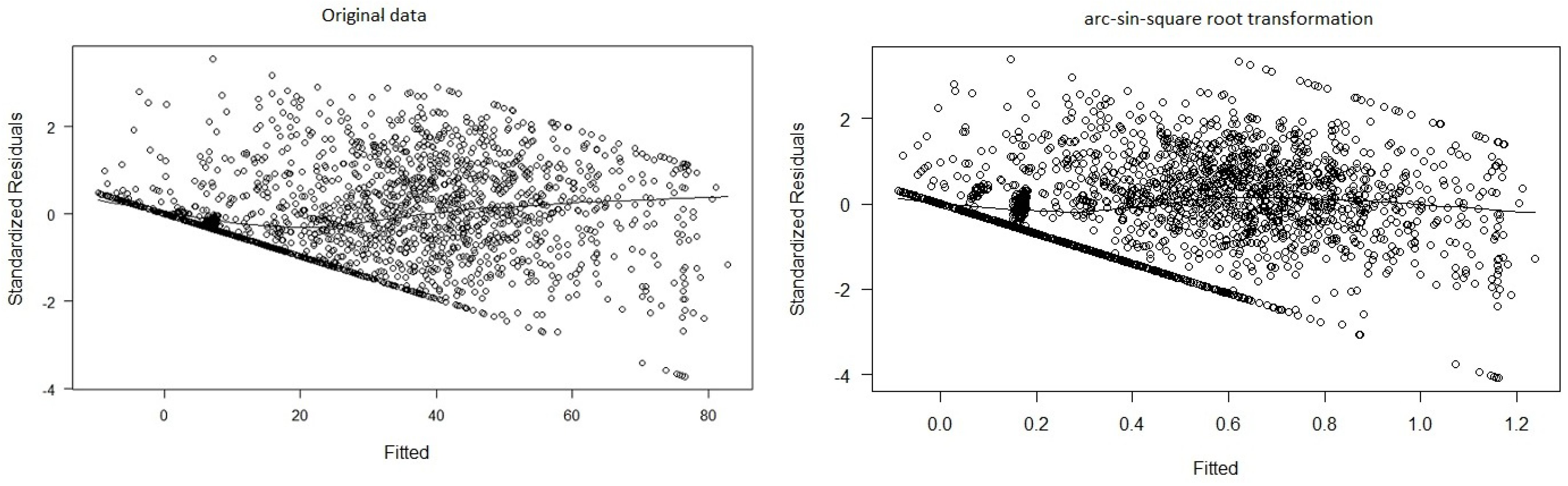
The first method used has been a linear regression model. However, a first analysis of the data set reveals problems in terms of heteroscedasticity (Breusch–Pagan’s p-value lower than 0.001) and normality (Shapiro–Wilk’s p-value lower than 0.001). We have checked several transformations of the response variable (Box–Cox transformations, where or or the arc-sin-square root transformation) but they got a higher dependency between the variance and the mean except for the arc-sin-square root transformation that got similar results than the raw data (Figure 1), so we decided to keep the original response variable for the sake of simplicity, taking into account the limitations of the regression model given the non-constant variance.
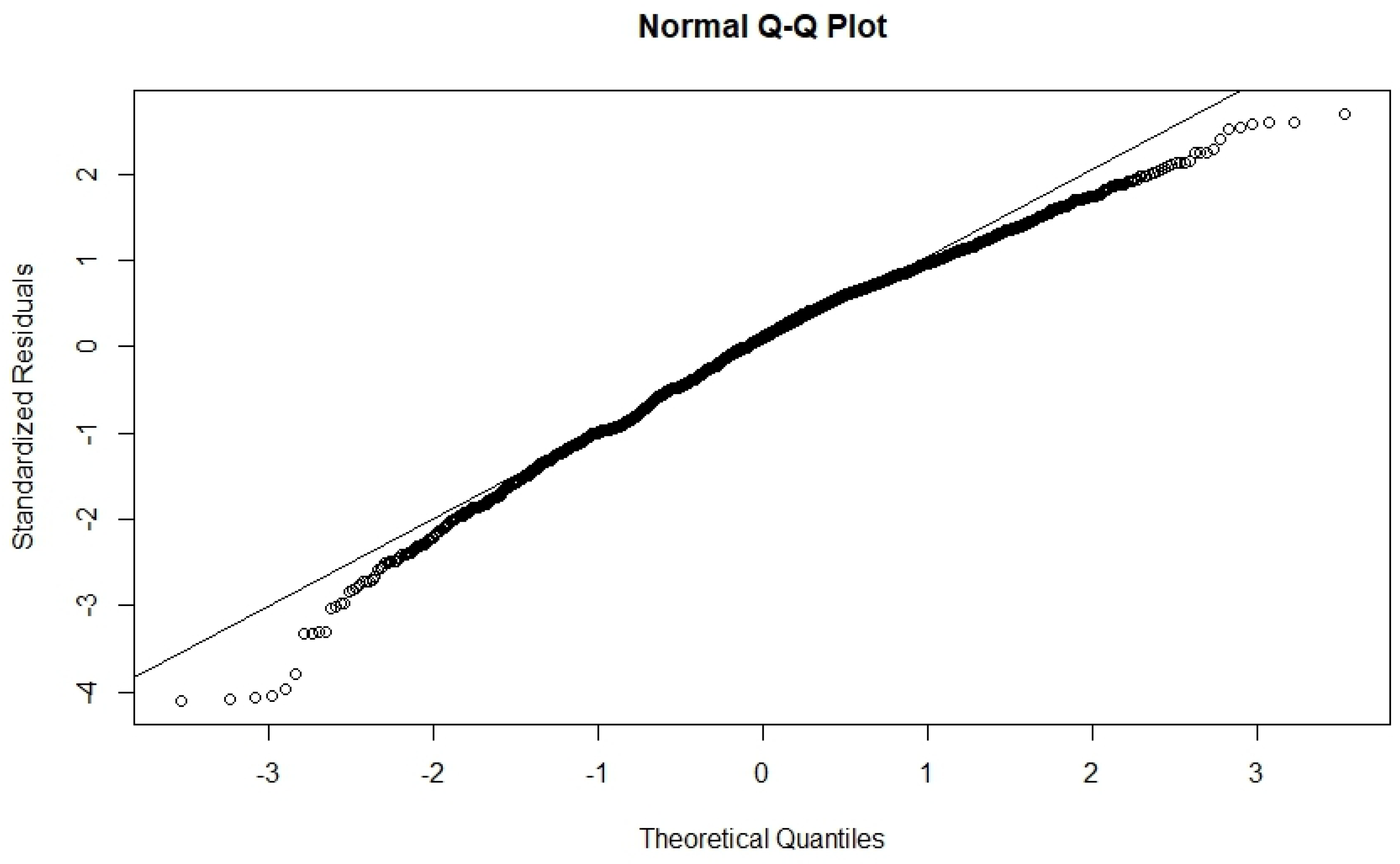
On the other hand, the QQ plot of the standardized residuals (see Figure 2) shows non-normal errors with the apparently long-tailed distribution. To address this problem, we have used robust regression models [27,28]. To choose the most suitable robust method for the estimation of the coefficients, we have compared the RMSE (root mean squared error) of the models fitted by using Huber’s M-estimator [29], the least trimmed squares (LTS) robust (high breakdown point) regression [30], least-absolute-deviations (LAD) regression [31] and the S-estimators proposed by Koller and Stahel [32]. We have used the MASS [33] and robustbase [34] R packages to fit the models.
Due to the problems with the requirements of the linear regression, we propose the use of quantile regression [35,36,37] which makes no assumption on the errors. Quantile regression estimates the conditional median (or any other quantile) of the response variable instead of the conditional mean estimated by linear regression. However, not only can the median be predicted but also any quantile from the response variable’s distribution, so we will try to predict the lowest (lower quartile) and highest marks (upper quartile, 80th and 90th percentile) in the final exam. As goodness of fit measurement, we have computed the coefficient proposed by Koenker and Machado [38], defined as one minus the ratio between the sum of absolute deviations in the fully parameterized model and the sum of absolute deviations in the null (non-conditional) quantile model.
2.1.2. Artificial Neural Networks
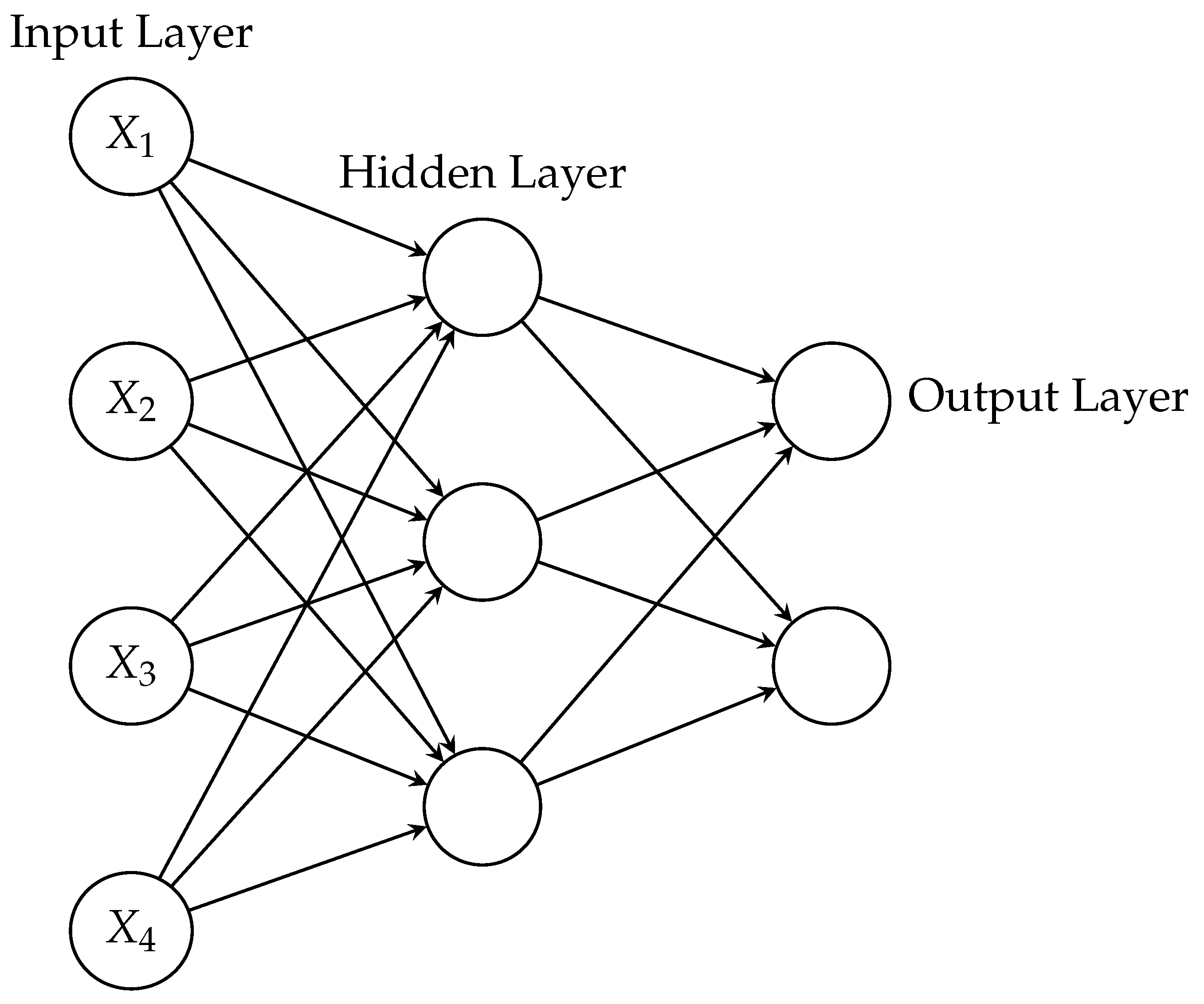
Our last attempt for the prediction of the mark obtained in the final exam was the use of Artificial Neural Networks (ANN). ANNs [39,40] are computational models which consist of nodes connected by links. The nodes, called neurons, are distributed in layers that can be divided into three classes: the first layer, called input layer, contains the nodes that represent the explanatory variables for the model; the last layer called output layer produces the result of the model; between the input and output layers the nodes are distributed in layers called hidden layers where the processing of the information is carried out. The nodes in each hidden layer are connected with all the neurons in the previous and next layers but there is no link between the nodes in the same layer. The number of hidden layers and the number of nodes in each one are hyperparameters that can be fixed by the research before training the ANN. Figure 3 shows the structure of an ANN with one hidden layer and three nodes in it.
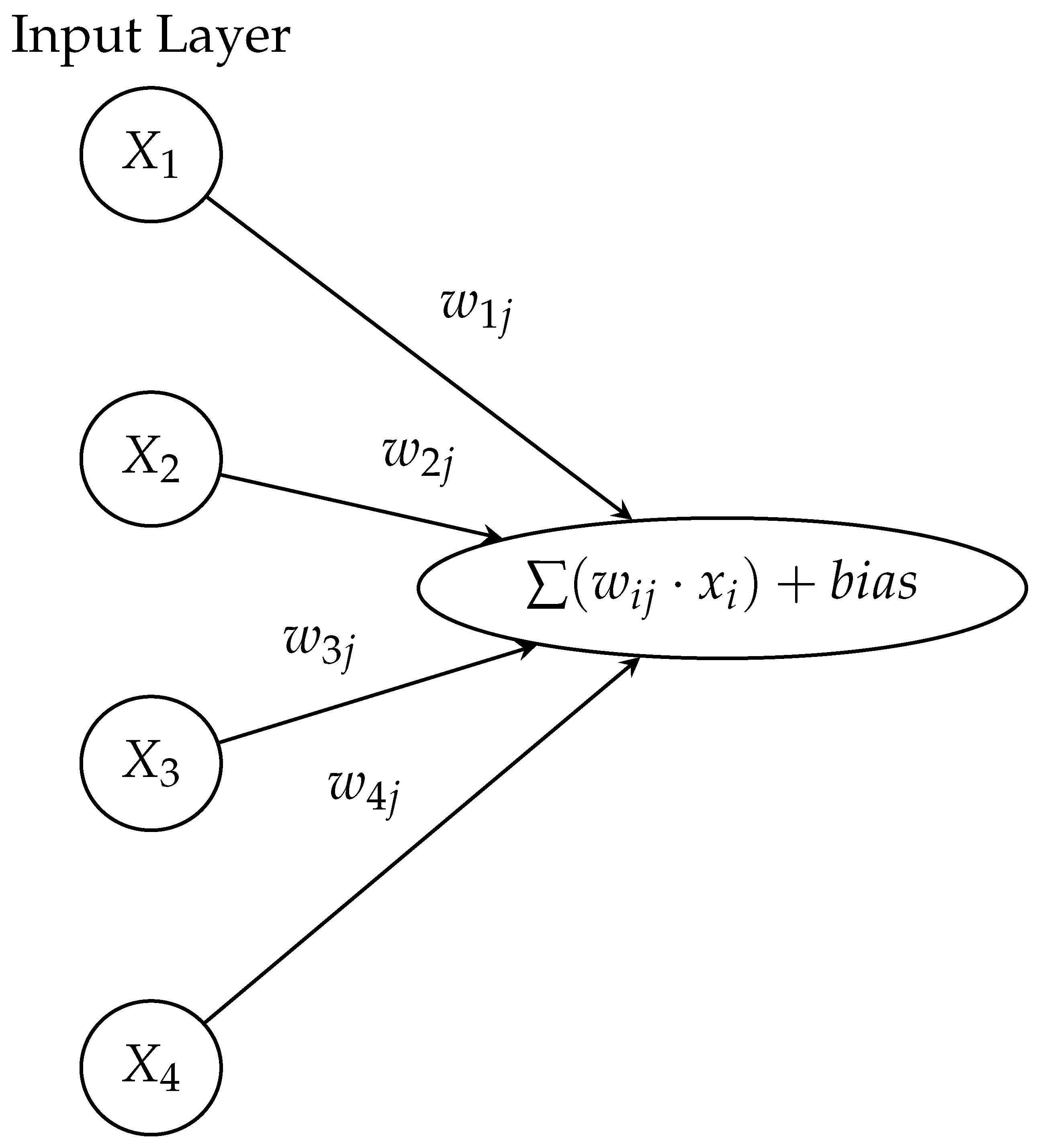
The processing of the information in the hidden layers is performed inside each neuron as follows: each link connecting two neurons i and j has associated a numerical parameter called weight and denoted , which determines how strongly the neuron i affects the neuron j. So, the information that a neuron j receives is the value taken by the neurons in the previous layer multiplied by the weights of the links plus a bias to adjust the information along with the weighted sum of the inputs to the neuron. Figure 4 illustrates the information received by the first neuron in the hidden layer of the ANN in Figure 3. The weights are estimated in the training of the ANN in such a way that the error of the output of the ANN is minimized.
A function is applied to the weighted sum of the inputs with the bias to produce the output of the neuron. This function is called the activation function and it decides whether the information in the neuron is important enough to be incorporated into the process. The activation function must be chosen by the researcher among a wide range of functions such as the identity, the logistic or sigmoid, the hyperbolic tangent, Rectified Linearity Units (ReLu) or Softmax functions, introducing the non-linearity in our model.
In this work, we used the most common type of ANN, the multilayer perceptron (MLP) [39]. We have trained nine different MLPs with one hidden layer and a total of 527 MLPs with two hidden layers varying the number of neurons in the layers. To learn each MLP, we used three activation functions: identity, ReLU and Softplus. The explanatory variable SHIFT was transformed into a 0–1 variable, whereas TEACHING was converted into three binary variables and the numeric variables were re-scaled to the interval [−1,1]. The assessment measure to choose the best model is the RMSE.
2.2. Multiclass Classification
As it is shown in Section 3, we were not able to accurately predict the mark in the final exam due to the high errors obtained in both regression models and ANNs so we decided to approach the problem as a classification task where the target variable EXAM is categorized into four classes: Fail, PassingGrade, GradeB and GradeA. As we did when training the ANNs for regression, the variable SHIFT is transformed into a 0-1 variable, TEACHING into three binary variables and WEIGHT and CONTINUOUS have been re-scaled to the interval [−1,1].
The first method used to classify the exam score of a student was an MLP with a logistic activation function. We trained different MLPs with one and two hidden layers varying the number of nodes in them. To assess the accuracy of the ANNs we computed the following performance metrics, where denotes the number of true positives, the number of true negatives, the false positives and the number of false negatives:
- Classification ACCURACY: ratio between the number of correct predictions and the total number of predictions
- GEOMETRIC MEAN (GM): tries to measure the equilibrium between the performance on classifying both the majority and the minority classes
- MATTHEW’S CORRELATION COEFFICIENT (MCC): takes on values in the range . A value of indicates that the model predicts all negatives as positives and vice versa (perfect negative correlation), indicates that the model predicts randomly (no correlation), and indicates perfect agreement. It is computed as
- YOUDEN’S INDEX (J): aggregates the values of specificity and sensitivity. It ranges between 0 and 1. J = 0 indicates that the classifier is useless whereas J = 1 indicates perfect agreement.
- COEH’S KAPPA SCORE (K): measures how much better the classifier is performing with respect to random classification according to the frequency of each class. It takes on values under or equal to 1, considering that the classifier is useless when and as acceptance criterium, we can consider a good performance when [41]. Its formula iswhere is the ratio of observed agreements and the expected agreements.
, and J are computed for each class of the response variable and the measure given is the weighted mean, using as weights the relative frequency of each class in the test data set.
Unlike , the metrics , , J and K take into account the difference in the size of the classes of the response variable in the test data set. As Table 2 shows, the Fail class contains over eight times more items than GradeB class and over 33 times more items than GradeA. Therefore, can be misleading, for instance, if the model only classifies properly the Fail class.
Besides ANNs, we have also addressed the classification problem using Bayesian networks.
Bayesian Networks
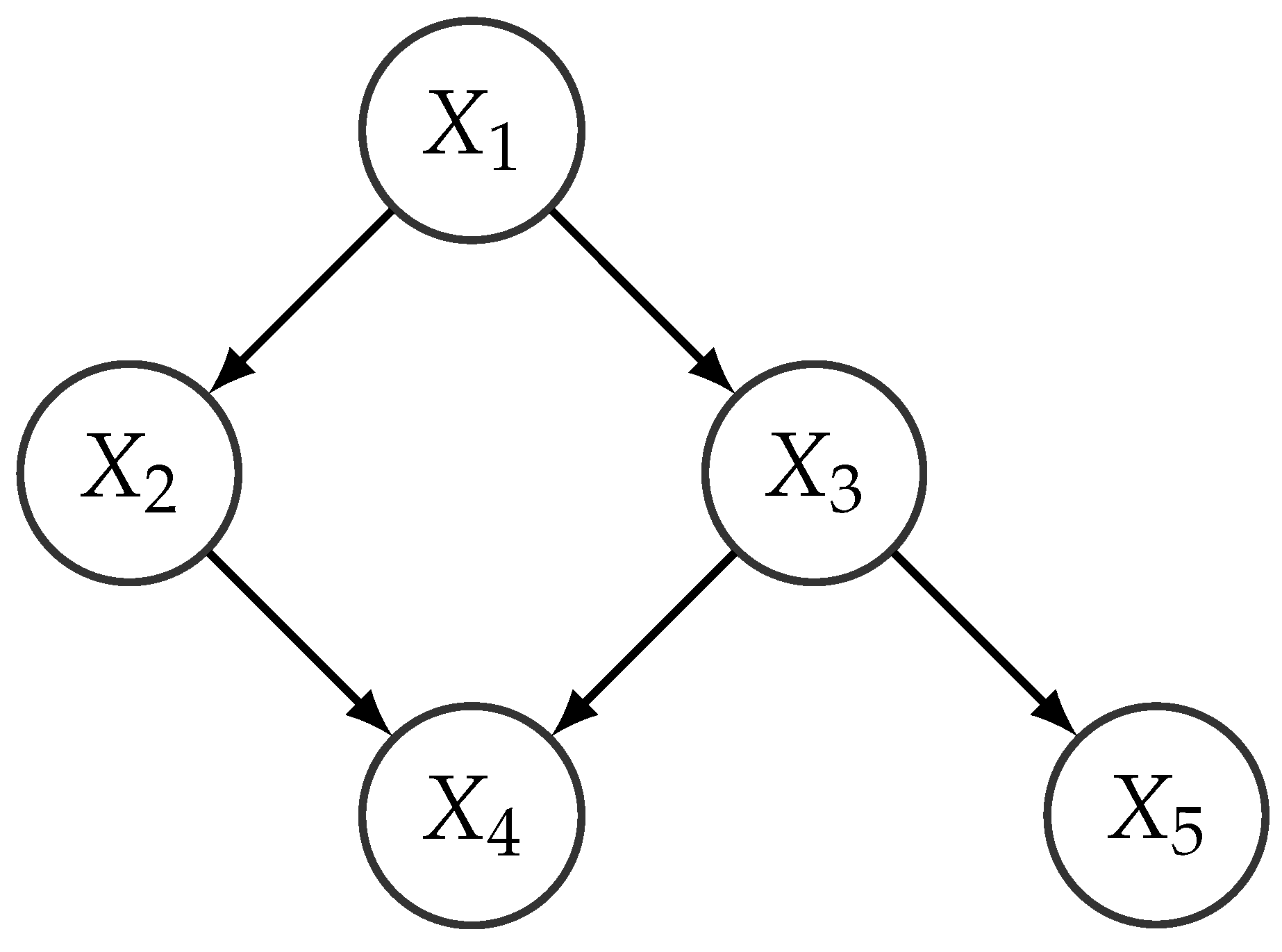
In what follows, we will use uppercase letters to denote random variables and lowercase letters to denote a value of a random variable. Boldfaced characters will be used to denote sets of variables. The set of all possible combinations of values of a set of random variables is denoted as . A Bayesian Network (BN) [42] with variables is formally defined as a directed acyclic graph with n nodes where each one corresponds to a variable in . Attached to each node , there is a conditional distribution of given its parents in the network, , so that the joint distribution of the random vector factorizes as
where denotes a configuration of the values of the parents of .
An example of a BN representing the joint distribution of the variables is shown in Figure 5. It encodes the factorization
A remarkable feature of BNs is their modularity, in the sense that the factorization simplifies the specification of large multivariate distributions that are replaced by a set of smaller ones (with a lower number of parameters to specify). For example, the factorization encoded by the network in Figure 5 replaces the specification of a joint distribution over 5 variables with the specification of 5 smaller distributions, each one of them with at most 3 variables. Another advantage is that the network structure describes the interaction between the variables in the model, in a way that can be easily interpretable, according to the d-separation criterion [42]. As an example, the structure in Figure 5 determines that variables and are independent if the value of is known, and likewise, and are independent if is known.
Building a BN from data involves two tasks: (i) learning the network structure and (ii) estimating the conditional distributions corresponding to the selected structure. Assuming that all the variables in the network are discrete or qualitative, maximum likelihood estimations of the conditional distributions can be obtained from the relative frequencies in the data of each combination of possible values of the variables involved. Structure learning [43] can be cast as an optimization problem, where the space of possible network structures is traversed trying to maximize some score function that measures how accurately a given structure fits the data. In this work, we have used the BIC score, which is a typical choice in the literature [44], defined as
where is the dataset, M is the network under evaluation, and is the joint distribution corresponding to network M, with parameters estimated by maximum likelihood. The idea of using the BIC score is to obtain networks that fit the data accurately while prioritizing simple networks. That is why the number of parameters, d, necessary to specify the probability distributions in the network, is used as a penalty factor. Other popular choices are the AIC and BDE scores [44]. In this paper, we have used the Hill Climbing (HC) optimization procedure with BIC score as a metric to optimize, using the implementation in the bnlearn [45] R package.
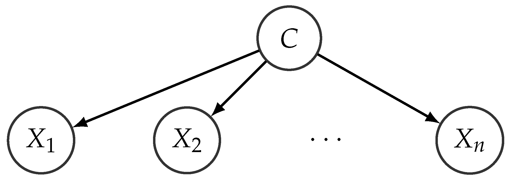
It is also possible to fix a given network structure beforehand, and only estimate the conditional distributions from data. This choice is typically adopted in practice when the network is going to be used for prediction purposes, where one could be more interested in the value of a target variable than in the interactions between the other variables. An example of such a fixed structure is the so-called Naive Bayes (NB) [46], where the variable whose value we want to predict is the root of the network and the only existing links go from that variable to the rest of the variables in the network (see Figure 6 for an example of such a structure).
NB structures impose a strong independence assumption (all the variables are conditionally independent given the root variable C), but in practice, it is compensated by the low number of parameters that need to be estimated from data. Notice that, in this case, the factorization encoded by the network results in
meaning that n one-dimensional conditional distributions must be specified, instead of one n-dimensional conditional distribution.
A BN can be used for classification by computing the posterior distribution of the class variable given an observed value of the predictive variables so that the result would be the value such that
Since , in the case of an NB structure, and taking into account Equation (8), it amounts to computing
Unlike the learning of MLPs, to train the BNs, the variable TEACHING is a unique variable with three categories: the rest of the variables (SHIFT, WEIGHT, CONTINUOUS and EXAM) are the same as the variables used with the MLPs.
2.3. Binary Classification
In an attempt to improve the reliability of the predictions, we have compared the performance of MLPs and BNs with a logistic regression model where the mark in the final exam is categorized into two classes: Fail and Pass. As in the previous section, the input variables for training the MLPs are: SHIFT (a 0–1 variable), TEACHING (split into three binary variables), WEIGHT and CONTINUOUS, both re-scaled to the interval [−1,1]. Twelve MLPs with one hidden layer have been learned varying the number of nodes in the intermediate layer from 3 to 14. The activation function used was the logistic.
To get the models based on BNs, we have trained a Naive Bayes model, as well as a BN with structure, learned using the HC optimization procedure with BIC score as a metric.
Finally, we compared the performance of the aforementioned classifiers with the results obtained by the logistic regression where the input variables are the same as those used with the MLP.
2.4. Prediction Using Degree as Explanatory Variable
In the last part of this study, we repeated the steps followed in the previous sections but introduced the degree program as an explanatory variable in an attempt to improve the quality of the predictions.
For the regression analysis, we fitted a linear model for each degree program in the study. We kept the rest of the explanatory variables with the following exceptions:
- In the linear model fitted for students enrolled in Industrial Engineering, Labor Relations and Physical Activity and Sport Science we have removed the variable WEIGHT from the model because it takes the same value in all the courses analyzed (30% in Industrial Engineering and 50% in both, Labor Relations and Physical Activity and Sport Science).
- In the linear model fitted in Industrial Engineering and Physical Activity and Sport Science the variable TEACHING is not used because the courses in these degrees were taught with the same methodology (in-person and eLearning, respectively).
The analysis of the standardized errors show lack of normality (Shapiro–Wilk’s p-value lower than 0.001) in all the degrees with exception of Mathematics, Public Management and Physical Activity and Sport Science (Shapiro–Wilks’ p-value = 0.1888, 0.1824 and 0.0575, respectively). Neither is the homoscedasticity requirement accomplished in all the degrees (Breusch–Pagan’s p-value under 0.001) except for I.T. Engineering (Breusch–Pagan’s p-value = 0.6045). Therefore, the coefficient of each model has been computed both by Least Squared Error and robust estimators and the RSME compared.
To learn the MLP the degree is entered as 7 binary variables while for the BNs the degree is one variable with 7 categories.
3. Results
3.1. Regression Results
Regarding the use of robust estimators to fit the linear model to our data, the resulting values of RMSE yield by the models estimated by Huber’s M-estimator, Least Trimmed Squares (LTS) robust regression, Least-Absolute-Deviations (LAD) regression and the S-estimator proposed by Koller and Stahel are displayed in Table 3. All the models except the one fitted by the LTS method are similar, getting the minimum RMSE with the estimations proposed by Koller and Stahel, so we will use this linear model to study the relationship between the explanatory variables and the mark obtained in the final exam. The results of this estimation are shown in Table 4.
Since the reference level for TEACHING is blended learning, the fitted regression within this group is
where SHIFT takes on the value 0 for the afternoon shift and 1 for courses in the morning shift.
When the course is taught online, there is no significant change in the model (p-value = 0.685) and the regression model when the course is taught face to face is
From these regression models, we can deduce that when the teaching is not in-person, students score lower in the final exam and, as was expected, students on the morning shift score higher than students on the afternoon shift.
The variable with the highest weight in the explanation of the mark obtained in the final exam (Table 5) is the score in the continuous evaluation followed by whether the type of teaching is “In-Person” and the shift. The percentage of the continuous evaluation in the assessment of the subject (WEIGHT) is the predictor with the lowest impact on the result of the final exam.
The robust residual standard error of the models in Equations (9) and (10) is that, together with the RMSE obtained when validating the model in the test data set (), indicates that the regression model fails at predicting accurately the mark in the final exam (which takes on values between 0 and 100). Thus, we tried quantile regression in an attempt to obtain better predictions of the mark in the final exam by predicting its median instead its mean as well as predictions for the lower and higher estimated marks.
The values of the goodness of fit measurement proposed by Koenker and Machado are shown in Table 6, suggesting that neither quantile regression model explains appropriately the scores in the final exam, especially for quantiles under the median.
The values of the coefficients, their standard error and p-values of the fitted models for the lower and upper quantiles ( and ), the median () and the 80th and 90th percentiles are displayed in Table 7.
The linear models to estimate the different percentiles for the mark in the exam of courses taught in-person are:
The linear models to estimate the different percentiles for the mark in the exam of blended courses taught (there are no significant differences between the models of online courses and blended courses except for the 90th percentile) are:
where SHIFT takes on the value 0 for the afternoon shift and 1 for courses in the morning shift.
Notice that the magnitude of the coefficients of variables WEIGHT and CONTINUOUS increases along with the percentile, whereas the higher the percentile is the lower the coefficient of SHIFT.
However, the RMSE for these models (Table 8) remains very large considering that the fitted models offer accurate predictions, particularly if we are interested in predicting low or high percentiles. This result is in line with the analysis made by Gonzalez et al. [25] in which no significant relation between the scores in CA and the final exam was found in the tails of the distribution. Neither does the estimate of the median by the quantile regression improve the accuracy of the estimation of the mean by the robust regression used in Equations (9) and (10).
Finally, we used MLPs for regression. More precisely, we trained nine MLPs with one hidden layer varying the number of nodes in the layer from 1 up to 21 and 527 MLPs with two hidden layers; the activation function used in all of them was the identity. The RMSE barely changes among all the MLPs achieving the minimum value (0.4082447) for the MLP with two neurons in the first hidden layer and 10 neurons in the second one. As the target variable EXAM was scaled to the interval , the RMSE obtained is the worst among the three methods of regression used in this study. When we used ReLU or Softplus as an activation function, the procedure did not converge.
Thus, the results indicate that it is not possible to predict in an accurate way the mark in the final exam from the explanatory variables selected in this study.
Our next attempt is to transform the regression problem into a classification problem.
3.2. Classification Results
In the fist attempt, we address a multiclass classification problem where the target variable is categorized into four classes (Fail, PassingGrade, GradeB and GradeA).
Table 9 displays the values of the performance measures obtained with the one hidden layer MLPs trained. MLPs with two hidden layers do not usually converge when six or more neurons are used in one of the layers while for structures with a low number of neurons the MLP is not able to classify classes either GradeB or GradeA. The low values of MCC, J and K indicate very poor performance of the classifier. The measure Accuracy reaches an acceptable value, but it is misleading because, as it is shown in the confusion matrix in Table 10, the MLP only predicts correctly the class Fail.
To compare the performance of the MLP with the BNs at classifying the exam mark, we trained a Naive Bayes structure and a BN with a structure determined using the HC algorithm. Table 11 and Table 12 display the performance values and the confusion matrix, respectively, for the Naive Bayes model. The BN trained with the HC method was not able to predict any category but Fail.
The performance of the Naive Bayes classifier is even worse than the MLP when predicting PassingGrade, GradeB and GradeA categories.
In the last attempt to improve the prediction of the students’ performance in the final exam, we ask if, at least, the fact of failing or passing the exam can be predicted from the continuous evaluation and the other variables considered. We have trained MLPs with one hidden layer and the logistic activation function, modifying the number of neurons in the hidden layer from 3 up to 14. Additionally, we trained a Naive Bayes classifier as well as a BN learned by the HC algorithm. Finally, we also tried logistic regression. Table 13 and Table 14 show the measures of performance and the confusion matrix of the three classifiers: the MLP with six neurons in the hidden layer (best performance achieved among the MLPs trained), the NB model and the results from the logistic regression. The BN learned by the HC algorithm was not able to predict the Pass category. In this case, the MLP accomplishes almost acceptable results and shows more superior behavior than the NB and the logistic regression. Logistic regression classifies better the Fail category but does not succeed in predicting the Pass category. NB has a similar performance to the MLP when predicting the fails but, as the logistic regression does, is unsuccessful with the students passing the exam.
To finish the study, we have added the degree to which the student is enrolled as an explanatory variable.
3.3. Improvement in the Accuracy When the Degree Is Added to the Previous Models
When the degree is introduced as a predictor in the linear models, the variable WEIGHT cannot be included for Industrial Engineering (whose value is 30% in all the cases), Labor Relations (50%) and Physical Activity and Sport Science (50%) as well as variable TEACHING neither can be included for Industrial Engineering (only in-person) nor Physical Activity and Sport Science (only e-learning). Only Economy and Mathematics have the three types of teaching, the rest (I.T, Labor Relations and Public Management) have been only taught by e-learning and in-person, taking as reference the e-learning group.
Table 15 shows the RSME of the different linear models depending on the estimator used to compute the coefficients of the linear model. Now, the robust estimators of the coefficients that minimize the RMSE depend on the degree program considered. If we compare the RMSE of the best choice with the results in Table 3 we can notice that the change in RMSE depends strongly on the degree: whereas in Economy the RMSE decreases about 20%, in others as I.T. or Mathematics it barely changes. In any case, the RMSEs remain high enough to consider the predictions reliable.
In Table 16, we can observe how the mark obtained in the CA contributes in a positive and significant way, no matter the degree. However, the weight of the CA in the assessment of the course has a negative effect on the degrees of Economy and Mathematics, being positive in the rest of the degrees. Moreover, it is remarkable that Mathematics is the only degree for which in-person teaching has a negative effect on the performance of the students in the final exam. This could be due to the sharpest peak in performance during the COVID pandemic in comparison with the rest of the degrees.
Regarding the multiclass classification task, Table 17 displays the performance measures of the MLP with eight neurons in the hidden layer (structure with the best performance among the twelve one-hidden-layer MLPs trained) and the NB classifier (BN learned with the HC method keeps on being unable to classify classes different from Fail. There is a noticeable improvement in the performance of both classifiers, especially in the MLP, although the assessment measures are still low.
If we reduce the problem to determine whether a student will pass or fail the final exam, Table 18 shows the performance of the three classifiers and the logistic regression. In this case, the BN learned with the HC algorithm is able to predict the passing students although its performance is poor. The results show how the MLP and the logistic regression improve their accuracy while the NB loses precision as a classifier.
4. Discussion
From the results detailed in Section 3, the prediction of the student performance in the final exam of a course is a difficult task. The variables used to explain the score in the final exam: shift, type of teaching, the weight of the continuous evaluation in the assessment of the subject and the performance of the students in the continuous evaluation, turn out to be insufficient to explain the score obtained in the final exam. The first issue that we face when trying to fit a linear model to the data is the difference in variability. This problem remains even when one regression model is fitted for each degree. The measures of error (Robust Residual Standard Error and RMSE) indicate that the regression model has no acceptable predictability, so there must be important variables in explaining the efficiency of the students when taking the final exam, that this study has not taken into account. These results are in agreement with the conclusions obtained in the studies of Bjælde et al. [23] and Day et al. [6]. However, the regression model shows that the student achievements in the continuous assessment play an important role in the final exam mark. Actually, it is the explanatory variable with the highest weight in the prediction of the final exam score followed by the fact of teaching the course face to face. This result agrees with findings in [25], Gidado [47], Onihunwa et al. [48] or Santos et al. [49]. Actually, every course at the University of Almeía has a mandatory CA in its assessment procedure which implies that the positive effect of the CA remains even when the rest of the courses taken by students have CA, as opposed to what Perez-Martínez et al. [50] infer from their studies.
From the regression models, we can also deduce that when the teaching is not in-person, students score lower in the final exam. This conclusion is opposed to the findings in the literature about the better performance of students during the COVID-19 outbreak [51,52,53]. A possible explanation for this different behavior could be that during the COVID-19 lockdown, the University of Almería fixed a mandatory 50% of CA in all the courses; the marks in the CA part are significantly higher in e-learning teaching (50.51% for e-learning against 36.5% got in in-person taught courses) lowering the motivation for exam preparation in some students as have been reported in [10,14,23]. This rise in online CA was also reported by De Santos Berbel et al. [54] but the authors also found a growth in the dropout rate, which could have a negative effect on the variable Exam because the student’s withdrawal is recorded in this variable with zero. Another possible explanation could be that there is more room for cheating in online CA: instructors could have made a bigger effort to avoid cheating in the online final exam by, for example, increasing the bank of questions or setting a tight completion time whereas in blended teaching the final exam is face to face. This could cause a larger gap between the marks obtained in the continuous assessment and in the final exam.
Neither quantile regression offers an accurate forecast of the final exam outcomes. The low values of the Koenker and Machado R index, especially in low percentiles, denote that the quantile model also fails in explaining the variability in the response variable. The RMSE of the forecast of the percentiles are high, particularly when fitting high percentiles in line with what was stated by Gonzalez et al. [25].
The use of ANNs to predict the mark in the final exam yields the worst result in comparison with the linear model and the quantile regression, almost doubling the RMSE of the estimations.
Splitting the grades in the final exam into four intervals to use classification procedures in an attempt to make predictions about the results of the exam neither improves the outcomes. The MLP with one hidden layer outperforms the NB increasing by more than 50% the assessment measures MCC and K and doubling the Youden’s index. Accuracy measure is similar in both methods because NB is able to properly predict the Fail category (more than 94.6% of agreements) but fails for higher categories, likely due to the limited number of cases in the dataset.
If the problem is reduced to just predicting whether a student will pass or fail the final exam, we obtain more accurate results, particularly by using the MLP, which outperforms both, NB and logistic regression, being able to rightly predict 61.7% of the students passing the exam (against the 52.5% of the NB and the 44.3% of the logistic regression). The three methods are accurate when predicting the failures: MLP predicts this class 86.7% of the time, NB 87.1% of the time and logistic regression 92.3%.
The inclusion of the degree read by the student barely improves the accuracy of the methods studied, which is in line with Pérez Martínez et al. [50] who suggest the improvement in the student’s performance does not depend on the degree.
5. Conclusions
Continuous evaluation has been adopted by most of the courses taught in Spanish universities due to, either academic decisions or because colleges or accreditation agencies make a percentage of CA in the assessment of the courses mandatory. There is no doubt about the benefits of including a CA in a course playing both roles: as summative and formative assessment, mainly when the continuous evaluation offers feedback to the students and they take advantage of that feedback. However, what is less clear is the magnitude of this positive effect on the learning of the students as well as on their results in the final exam of the course in that case. Furthermore, there is no evidence about whether the benefits of the CA outweigh the increase in the workload of students and teachers.
There is a number of papers in the literature studying the relationship between the continuous assessment and the final exam mark [21,23,24,25,47,48,49], but the statistical procedures used are traditional: descriptive Statistics, T tests, Pearson’s correlation test, ANOVA or linear regression. In this study, we have tried to find statistical evidence about whether the effect of the CA is a determinant in students’ performance on the final exam by using and comparing state-of-the-art methods as it is suggested by [55]. Although it has been shown that CA has actually an effect on the final exam score, this effect is not decisive to predict how a student will perform in the final exam.
The results obtained seem to encourage the instructors to move CA activities closer to the final exam requirements. Given that the weight of the CA in the assessment of the course has a positive effect on the fitted regression model, the increase in this percentage could enhance students’ performance in the final exam. Moreover, the type of CA used in the course could be a variable to take into account when it comes to improving the students’ learning, despite there is no agreement in the literature about this point: Day et al. [6] found no differences in the students’ scores on courses with different assessment types while Deeley et al. [18] assert that diverse assessment with a more flexible approach and assessment method that let the students be actively involved in making choices about their assessment would increase students’ motivation. The large differences in the regression models fitted for each degree suggest that the design of the assessment must be customized to match the student’s characteristics.
Supplementary Materials
The following supporting information can be downloaded at: https://0-www-mdpi-com.brum.beds.ac.uk/article/10.3390/math10213994/s1.
Author Contributions
Conceptualization, A.D.M., A.R.M., M.M., R.R. and A.S.; methodology, A.D.M., M.M. and A.S.; software, M.M. and A.S.; validation, M.M. and A.S.; formal analysis, M.M. and A.S.; investigation, M.M. and A.S.; resources, A.D.M., M.M. and A.S.; data curation, A.D.M., M.M. and A.S.; writing—original draft preparation, M.M. and A.S.; writing—review and editing, A.D.M., M.M. and A.S.; visualization, A.D.M., M.M. and A.S.; supervision, M.M. and A.S.; project administration, M.M., R.R. and A.S.; funding acquisition, R.R. and A.S. All authors have read and agreed to the published version of the manuscript.
Funding
This research is part of Project PID2019-106758GB-C32 funded by MCIN/AEI/10.13039/501100011033, FEDER “Una manera de hacer Europa” funds. This research is also partially funded by Junta de Andalucía grant P20-00091 and University of Almería grant UAL2020-FQM-B196.
Data Availability Statement
Training and test data sets used in this research are available as Supplementary Materials.
Acknowledgments
We would like to acknowledge the support given by the Vice-chancellorship for Academic planning of the University of Almería.
Conflicts of Interest
The authors declare no conflict of interest.
Abbreviations
The following abbreviations are used in this manuscript:
| AFL | Assessment for Learning |
| ANN | Artificial Neural Network |
| BN | Bayesian Network |
| CA | Continuous Assessment |
| DAG | Directed acyclic graph |
| GM | Geometric Mean |
| HC | Hill-climbing |
| J | Youden’s index |
| K | Coeh’s kappa score |
| KS | Koller and Stahel robust estimator |
| LAD | least-absolute-deviations regression |
| LTS | Least trimmed squares robust regression |
| MCC | Matthew’s correlation coefficient |
| MLP | Multilayer perceptron |
| NB | Naive Bayes |
| RMSE | Root mean square error |
| TAN | Tree augmented network |
References
- McDowell, L.; Wakelin, D.; Montgomery, C.; King, S. Does assessment for learning make a difference? The development of a questionnaire to explore the student response. Assess. Eval. High. Educ. 2011, 36, 749–765. [Google Scholar] [CrossRef]
- Sambell, K.; McDowell, L.; Montgomery, C. Assessment for Learning in Higher Education; Routledge: Oxfordshire, UK, 2012. [Google Scholar]
- Zlatkin-Troitschanskaia, O.; Shavelson, R.J.; Pant, H.A. Assessment of learning outcomes in higher education: International comparisons and perspectives. In Handbook on Measurement, Assessment, and Evaluation in Higher Education; Routledge: Oxfordshire, UK, 2017; pp. 686–698. [Google Scholar]
- Zahl, S.; Jimenez, S.; Huffman, M. Assessment at the highest degree(s): Trends in graduate and professional education. In Trends in Assessment: Ideas, Opportunities, and Issues for Higher Education; Stylus: Sterling, TX, USA, 2019. [Google Scholar]
- Nair, P.; Pillay, J. Exploring the validity of the continuous assessment strategy in higher education institutions: Research in higher education. South Afr. J. High. Educ. 2004, 18, 302–312. [Google Scholar]
- Day, I.N.; van Blankenstein, F.M.; Westenberg, P.M.; Admiraal, W.F. Explaining individual student success using continuous assessment types and student characteristics. High. Educ. Res. Dev. 2018, 37, 937–951. [Google Scholar] [CrossRef]
- Poza-Lujan, J.L.; Calafate, C.T.; Posadas-Yagüe, J.L.; Cano, J.C. Assessing the impact of continuous evaluation strategies: Tradeoff between student performance and instructor effort. IEEE Trans. Educ. 2015, 59, 17–23. [Google Scholar] [CrossRef] [Green Version]
- Combrinck, M.; Hatch, M. Students’ experiences of a continuous assessment approach at a Higher Education Institution. J. Soc. Sci. 2012, 33, 81–89. [Google Scholar] [CrossRef]
- Shields, S. ‘My work is bleeding’: Exploring students’ emotional responses to first-year assignment feedback. Teach. High. Educ. 2015, 20, 614–624. [Google Scholar] [CrossRef]
- Bloxham, S.; Boyd, P. Developing Effective Assessment In Higher Education: A Practical Guide; McGraw-Hill Education: New York, NY, USA, 2007. [Google Scholar]
- Holmes, N. Student perceptions of their learning and engagement in response to the use of a continuous e-assessment in an undergraduate module. Assess. Eval. High. Educ. 2015, 40, 1–14. [Google Scholar] [CrossRef]
- Hernández, R. Does continuous assessment in higher education support student learning? High. Educ. 2012, 64, 489–502. [Google Scholar] [CrossRef] [Green Version]
- Holmes, N. Engaging with assessment: Increasing student engagement through continuous assessment. Act. Learn. High. Educ. 2018, 19, 23–34. [Google Scholar] [CrossRef] [Green Version]
- Martín-Carrasco, F.; Granados, A.; Santillan, D.; Mediero, L. Continuous Assessment in Civil Engineering Education-Yes, but with Some Conditions. CSEDU 2014, 2, 103–109. [Google Scholar]
- Rubio-Escudero, C.; Asencio-Cortés, G.; Martínez-Álvarez, F.; Troncoso, A.; Riquelme, J.C. Impact of auto-evaluation tests as part of the continuous evaluation in programming courses. In Proceedings of the 13th International Conference on Soft Computing Models in Industrial and Environmental Applications, San Sebastian, Spain, 6–8 June 2018; pp. 553–561. [Google Scholar]
- López-Tocón, I. Moodle Quizzes as a Continuous Assessment in Higher Education: An Exploratory Approach in Physical Chemistry. Educ. Sci. 2021, 11, 500. [Google Scholar] [CrossRef]
- Carless, D.; Salter, D.; Yang, M.; Lam, J. Developing sustainable feedback practices. Stud. High. Educ. 2011, 36, 395–407. [Google Scholar] [CrossRef]
- Deeley, S.J.; Fischbacher-Smith, M.; Karadzhov, D.; Koristashevskaya, E. Exploring the ‘wicked’ problem of student dissatisfaction with assessment and feedback in higher education. High. Educ. Pedagog. 2019, 4, 385–405. [Google Scholar] [CrossRef]
- Scott, G.W. Active engagement with assessment and feedback can improve group-work outcomes and boost student confidence. High. Educ. Pedagog. 2017, 2, 1–13. [Google Scholar] [CrossRef] [Green Version]
- Dejene, W. The practice of modularized curriculum in higher education institution: Active learning and continuous assessment in focus. Cogent Educ. 2019, 6, 1611052. [Google Scholar] [CrossRef]
- Sanz-Pérez, E. Students’ performance and perceptions on continuous assessment. Redefining a chemical engineering subject in the European higher education area. Educ. Chem. Eng. 2019, 28, 13–24. [Google Scholar] [CrossRef]
- Gibbs, G. How assessment frames student learning. In Innovative Assessment in Higher Education; Routledge: Oxfordshire, UK, 2006; pp. 43–56. [Google Scholar]
- Bjælde, O.E.; Jørgensen, T.H.; Lindberg, A.B. Continuous assessment in higher education in Denmark. Dan. Univ. Tidsskr. 2017, 12, 1–19. [Google Scholar] [CrossRef]
- Reina-Paz, M.D.; Rodriguez-Oromendia, A.; Sevilla-Sevilla, C. Effect of Continuous Assessment Tests on Overall Student Performance in the Case of the Spanish National Distance Education University (UNED). J. Int. Educ. Res. (JIER) 2014, 10, 61–68. [Google Scholar] [CrossRef]
- Gonzalez, M.d.l.O.; Jareño, F.; López, R. Impact of students’ behavior on continuous assessment in Higher Education. Innov. Eur. J. Soc. Sci. Res. 2015, 28, 498–507. [Google Scholar] [CrossRef]
- Gil-Begue, S.; Bielza, C.; Larrañaga, P. Multi-dimensional Bayesian network classifiers: A survey. Artif. Intell. Rev. 2021, 54, 519–559. [Google Scholar] [CrossRef]
- Li, G. Robust regression. Explor. Data Tables Trends Shapes 1985, 281, U340. [Google Scholar]
- Faraway, J.J. Linear Models with R; CRC: Boca Raton, FL, USA, 2004. [Google Scholar]
- Huber, P.J. Robust Estimation of a Location Parameter. Ann. Math. Stat. 1964, 35, 73–101. [Google Scholar] [CrossRef]
- Giloni, A.; Padberg, M. Least trimmed squares regression, least median squares regression, and mathematical programming. Math. Comput. Model. 2002, 35, 1043–1060. [Google Scholar] [CrossRef]
- Thanoon, F.H. Robust regression by least absolute deviations method. Int. J. Stat. Appl. 2015, 5, 109–112. [Google Scholar]
- Koller, M.; Stahel, W.A. Nonsingular subsampling for regression S estimators with categorical predictors. Comput. Stat. 2017, 32, 631–646. [Google Scholar] [CrossRef]
- Ripley, B.; Venables, B.; Bates, D.M.; Hornik, K.; Gebhardt, A.; Firth, D.; Ripley, M.B. Package ‘mass’. Cran R 2013, 538, 113–120. [Google Scholar]
- Maechler, M.; Rousseeuw, P.; Croux, C.; Todorov, V.; Ruckstuhl, A.; Salibian-Barrera, M.; Verbeke, T.; Koller, M.; Conceicao, E.L.; di Palma, M.A. Package ‘Robustbase’. 2022. Available online: https://cran.r-project.org/web/packages/robustbase/index.html (accessed on 10 October 2021).
- Koenker, R.; Hallock, K.F. Quantile regression. J. Econ. Perspect. 2001, 15, 143–156. [Google Scholar] [CrossRef]
- Hao, L.; Naiman, D.Q. Quantile Regression; Number 149; Sage: Thousand Oaks, CA, USA, 2007. [Google Scholar]
- Yu, K.; Lu, Z.; Stander, J. Quantile regression: Applications and current research areas. J. R. Stat. Soc. Ser. 2003, 52, 331–350. [Google Scholar] [CrossRef]
- Koenker, R.; Machado, J.A. Goodness of fit and related inference processes for quantile regression. J. Am. Stat. Assoc. 1999, 94, 1296–1310. [Google Scholar] [CrossRef]
- Haykin, S. Neural Networks: A Comprehensive Foundation; Prentice Hall: Hoboken, NJ, USA, 1998. [Google Scholar]
- Goodfellow, I.; Bengio, Y.; Courville, A. Deep Learning; MIT Press: Cambridge, MA, USA, 2016. [Google Scholar]
- Landis, J.R.; Koch, G.G. The measurement of observer agreement for categorical data. Biometrics 1977, 1, 159–174. [Google Scholar] [CrossRef] [Green Version]
- Pearl, J. Probabilistic Reasoning in Intelligent Systems; Morgan-Kaufmann: San Mateo, CA, USA, 1988. [Google Scholar]
- Scanagatta, M.; Salmerón, A.; Stella, F. A survey on Bayesian network structure learning from data. Prog. Artif. Intell. 2019, 8, 425–439. [Google Scholar] [CrossRef]
- Neapolitan, R.E. Learning Bayesian Networks; Prentice Hall: Hoboken, NJ, USA, 2003. [Google Scholar]
- Scutari, M. Learning Bayesian Networks with the bnlearn R Package. J. Stat. Softw. 2010, 35, 1–22. [Google Scholar] [CrossRef] [Green Version]
- Friedman, N.; Geiger, D.; Goldszmidt, M. Bayesian Network Classifiers. Mach. Learn. 1997, 29, 131–163. [Google Scholar] [CrossRef] [Green Version]
- Gidado, B.K. The corelation between continuous assessment and examination scores of public administration students of the University of Abuja. Sokoto Educ. Rev. 2021, 20, 12–20. [Google Scholar]
- Onihunwa, J.; Adigun, O.; Irunokhai, E.; Sada, Y.; Jeje, A.; Adeyemi, O.; Adesina, O. Roles of Continuous Assessment Scores in Determining the Academic Performance of Computer Science Students in Federal College of Wildlife Management. Am. J. Eng. Res. 2018, 7, 7–20. [Google Scholar]
- Santos, J.M.; Ortiz, E.; Marín, S. Variation indexes of marks due to continuous assessment. Empirical approach at university/Índices de variación de la nota debidos a la evaluación continua. Contrastación empírica en la enseñanza universitaria. Cult. Educ. 2018, 30, 491–527. [Google Scholar] [CrossRef]
- Pérez-Martínez, J.E.; García-García, M.J.; Perdomo, W.H.; Villamide-Díaz, M.J. Analysis of the results of the continuous assessment in the adaptation of the Universidad Politécnica de Madrid to the European Higher Education Area. In Proceedings of the Research in Engineering Education Symposium, Palm Cove, QLD, Australia, 20–23 July 2009; Volume 90. [Google Scholar]
- Gonzalez, T.; De La Rubia, M.A.; Hincz, K.P.; Comas-Lopez, M.; Subirats, L.; Fort, S.; Sacha, G.M. Influence of COVID-19 confinement on students’ performance in higher education. PLoS ONE 2020, 15, e0239490. [Google Scholar] [CrossRef]
- Iglesias-Pradas, S.; Hernández-García, Á.; Chaparro-Peláez, J.; Prieto, J.L. Emergency remote teaching and students’ academic performance in higher education during the COVID-19 pandemic: A case study. Comput. Hum. Behav. 2021, 119, 106713. [Google Scholar] [CrossRef]
- Moravec, L.; Ječmínek, J.; Kukalová, G. Evaluation of final examination performance at Czech University of Life Sciences during the COVID-19 outbreak. J. Effic. Responsib. Educ. Sci. 2022, 15, 47–52. [Google Scholar] [CrossRef]
- De Santos-Berbel, C.; Hernando García, J.I.; De Santos Berbel, L. Undergraduate Student Performance in a Structural Analysis Course: Continuous Assessment before and after the COVID-19 Outbreak. Educ. Sci. 2022, 12, 561. [Google Scholar] [CrossRef]
- Yang, X.; Ge, J. Predicting Student Learning Effectiveness in Higher Education Based on Big Data Analysis. Mob. Inf. Syst. 2022, 2022, 8409780. [Google Scholar] [CrossRef]
Figure 1.
Standardized residuals versus fitted values with the original data and after transforming by arc−sin−square root.
Figure 1.
Standardized residuals versus fitted values with the original data and after transforming by arc−sin−square root.

Figure 2.
QQ—plot of the standardized residuals.

Figure 3.
An example of an ANN with one hidden layer.

Figure 4.
An example of the information received by a neuron in the hidden layer.

Figure 5.
An example of a BN structure with 5 variables.

Figure 6.
A Naive Bayes structure with n predictive variables and class C.


Table 1.
Frequency distribution of some explanatory variables in the data set.
| Shift | Type of Teaching | Weight |
|---|---|---|
| Morning 1236 Afternoon 1161 | In-person 1239 E-learning 781 Blended 377 | 20% 47 30% 800 40% 166 50% 1192 60% 192 |
Table 2.
Frequency distribution of the categorized variable EXAM in the test data set.
| Class | |
|---|---|
| Fail | 504 |
| PassingGrade | 106 |
| GradeB | 62 |
| GradeA | 15 |
Table 3.
Comparison of the RMSE obtained by the different methods of estimation: Huber = Huber’s M-estimator, LTS = least trimmed squares robust regression, LAD = least-absolute-deviations regression and KS = S-estimator proposed by Koller and Stahel.
Table 3.
Comparison of the RMSE obtained by the different methods of estimation: Huber = Huber’s M-estimator, LTS = least trimmed squares robust regression, LAD = least-absolute-deviations regression and KS = S-estimator proposed by Koller and Stahel.
| Method of Estimation | RMSE |
|---|---|
| Huber | 20.44772 |
| LTS | 40.45228 |
| LAD | 20.49332 |
| KS | 20.43824 |
Table 4.
Estimations of the regression coefficients using the KS estimator.
| Parameter | Value | Std.Error | t Value | p-Value |
|---|---|---|---|---|
| Intercept | −45.76676 | 3.61698 | −12.653 | <2 × 10 |
| SHIFTMorning | 10.16746 | 1.09684 | 9.270 | <2 × 10 |
| TEACHINGe-learning | 0.64087 | 1.58107 | 0.405 | 0.685 |
| TEACHINGIn-person | 18.69717 | 1.66811 | 11.209 | <2 × 10 |
| WEIGHT | 0.70788 | 0.06454 | 10.968 | < 2 × 10 |
| CONTINUOUS | 0.69939 | 0.01883 | 37.143 | <2 × 10 |
Table 5.
Standardized coefficient estimated by the S-estimator proposed by Koller and Stahel.
| Intercept | SHIFT | TEACHING e-Learning | TEACHINGIn-Person | WEIGHT | CONTINUOUS |
|---|---|---|---|---|---|
| −0.5254 | 0.3435 | 0.0217 | 0.6318 | 0.2550 | 0.6682 |
Table 6.
Goodness of fit of quantile regression for determined percentiles.
| 0.0002697 | 0.1134626 | 0.1761121 | 0.3841547 | 0.3940505 | 0.3801269 | 0.3402591 |
Table 7.
Coefficients of the quantile regression for , , , and .
| Intercept | SHIFT | TEACHINGe-Learning | TEACHINGIn-Person | WEIGHT | CONTINUOUS | ||
|---|---|---|---|---|---|---|---|
| Value | −28.15909 | 8.45455 | −0.81818 | 9.18182 | 0.34136 | 0.45455 | |
| Std.Error | 3.52704 | 0.78454 | 0.85138 | 1.44456 | 0.06642 | 0.02121 | |
| p-value | <0.001 | <0.001 | 0.33669 | <0.001 | <0.001 | <0.001 | |
| Value | −37.01504 | 8.31228 | −1.81706 | 13.00710 | 0.57015 | 0.72903 | |
| Std.Error | 4.30834 | 0.98214 | 1.29218 | 1.64289 | 0.07828 | 0.02158 | |
| p-value | <0.001 | <0.001 | 0.15985 | <0.001 | <0.001 | <0.001 | |
| Value | −40.59302 | 4.07737 | 1.84492 | 18.05048 | 0.75142 | 0.90754 | |
| Std.Error | 2.98465 | 0.86038 | 1.59524 | 1.27903 | 0.05460 | 0.01913 | |
| p-value | <0.001 | <0.001 | 0.24763 | <0.001 | <0.001 | <0.001 | |
| Value | −38.15904 | 4.24812 | 1.42903 | 16.12104 | 0.73460 | 0.95913 | |
| Std.Error | 5.38077 | 1.58888 | 2.17907 | 2.08862 | 0.10189 | 0.02961 | |
| p-value | <0.001 | 0.00757 | 0.51204 | <0.001 | <0.001 | <0.001 | |
| Value | −39.51856 | 7.91199 | 14.70176 | 28.41365 | 0.79037 | 0.92436 | |
| Std.Error | 7.51783 | 1.97941 | 2.27543 | 2.81211 | 0.14375 | 0.03541 | |
| p-value | <0.001 | <0.001 | <0.001 | <0.001 | <0.001 | <0.001 |
Table 8.
Root mean square error (RMSE) of quantile regression models for , , , and .
| 26.09989 | 20.49223 | 24.42311 | 26.12923 | 34.35438 |
Table 9.
Performance 1 of MLP with one hidden layer.
| Neurons | Accuracy | GM | MCC | J | K |
|---|---|---|---|---|---|
| 4 | 0.7423581 | 0.3767619 | 0.1912527 | 0.1126921 | 0.2307464 |
| 5 | 0.7379913 | 0.4528189 | 0.2253644 | 0.16143641 | 0.2574133 |
| 6 | 0.7336245 | 0.3500356 | 0.1491623 | 0.08828901 | 0.2047303 |
| 7 | 0.7423581 | 0.3556055 | 0.1814024 | 0.10156554 | 0.2145427 |
| 8 | 0.7365357 | 0.3506387 | 0.1600189 | 0.09149303 | 0.2081272 |
| 9 | 0.7481805 | 0.4758372 | 0.2611203 | 0.18915434 | 0.2929113 |
| 10 | 0.7190684 | 0.4247192 | 0.1597665 | 0.12140248 | 0.2293730 |
| 15 | 0.7350801 | 0.4675948 | 0.2243916 | 0.1694903 | 0.275774 |
1 GM = Geometric, MCC = Matthew’s correlation coefficient, J = Youden’s Index and K = Coeh’s Kappa Score.
Table 10.
Confusion matrix obtained from the one-hidden layer MLP with 9 neurons.
| Predicted | |||||
|---|---|---|---|---|---|
| Fail | PassingGrade | GradeB | GradeA | ||
| Observed | Fail | 472 | 27 | 3 | 2 |
| PassingGrade | 75 | 25 | 4 | 2 | |
| GradeB | 37 | 13 | 6 | 6 | |
| GradeA | 6 | 6 | 1 | 2 | |
Table 11.
Performance 1 of the Naive Bayes classifier.
| Accuracy | GM | MCC | J | K |
|---|---|---|---|---|
| 0.7263464 | 0.3564184 | 0.1386113 | 0.08551829 | 0.1859933 |
1 GM = Geometric, MCC = Matthew’s correlation coefficient, J = Youden’s Index and K = Coeh’s Kappa Score.
Table 12.
Confusion matrix obtained from the Naive Bayes classifier.
| Predicted | |||||
|---|---|---|---|---|---|
| Fail | PassingGrade | GradeB | GradeA | ||
| Observed | Fail | 477 | 19 | 1 | 7 |
| PassingGrade | 83 | 18 | 2 | 3 | |
| GradeB | 38 | 14 | 3 | 7 | |
| GradeA | 11 | 3 | 0 | 1 | |
Table 13.
Assessment 1 of the classifiers MLP, NB and logistic regression.
| Accuracy | GM | MCC | J | K | |
|---|---|---|---|---|---|
| MLP | 0.8195051 | 0.7660164 | 0.5414379 | 0.5451470 | 0.5413786 |
| NB | 0.7787482 | 0.6759694 | 0.4128719 | 0.3956219 | 0.4113708 |
| Log.Reg. | 0.7947598 | 0.6390402 | 0.4252452 | 0.365242 | 0.4102143 |
1 GM = Geometric, MCC = Matthew’s correlation coefficient, J = Youden’s Index and K = Coeh’s Kappa Score.
Table 14.
Confusion matrices obtained from the classifiers MLP, NB and logistic regression.
| MLP | NB | Log.Reg. | |||||||||
|---|---|---|---|---|---|---|---|---|---|---|---|
| Predicted | Predicted | Predicted | |||||||||
| Fail | Pass | Fail | Pass | Fail | Pass | ||||||
| Observed | Fail | 437 | 67 | Observed | Fail | 439 | 65 | Observed | Fail | 465 | 39 |
| Pass | 70 | 113 | Pass | 87 | 96 | Pass | 102 | 81 | |||
Table 15.
Comparison of the RMSE obtained by the different methods of estimation in each degree: Huber = Huber’s M-estimator, LTS = least trimmed squares robust regression, LAD = least-absolute-deviations regression and KS = S-estimator proposed by Koller and Stahel.
Table 15.
Comparison of the RMSE obtained by the different methods of estimation in each degree: Huber = Huber’s M-estimator, LTS = least trimmed squares robust regression, LAD = least-absolute-deviations regression and KS = S-estimator proposed by Koller and Stahel.
| Method of Estimation | ||||
|---|---|---|---|---|
| Degree | Huber | LTS | KS | LAD |
| Economy | 16.25501 | 31.41839 | 16.23750 | 16.54850 |
| I.T. | 22.30481 | 31.54442 | 22.30931 | 23.04748 |
| INDUS | 14.81322 | 20.37739 | 14.76142 | 14.50819 |
| Mathematics | 19.65349 | 42.74780 | 19.70359 | 20.22910 |
| Public Management | 18.23688 | 28.85815 | 17.99737 | 31.80174 |
| Labour Relations | 12.72984 | 33.55746 | 12.47861 | |
| Sports | 19.07092 | 18.70723 | 19.07724 | 21.53974 |
Table 16.
Coefficients of the regression model fitted for each degree. Inside the parenthesis not significant coefficients.
Table 16.
Coefficients of the regression model fitted for each degree. Inside the parenthesis not significant coefficients.
| Degree | Intercept | Teaching | Teaching | Weight | Continuous |
|---|---|---|---|---|---|
| e-Learning | In-Person | ||||
| Economy | 13.70546 | −3.89268 | (1.36264) | −0.40290 | 0.64196 |
| I.T. | −33.2755 | - | 19.2129 | 0.7942 | 0.5798 |
| INDUS | (0) | - | - | - | 0.40710 |
| Mathematics | 272.1077 | 15.9608 | −49.8121 | −5.7813 | 1.0668 |
| Public Management | −70.39375 | - | 20.32998 | 1.04353 | 0.88170 |
| Labour Relations | −8.99644 | - | 5.04751 | 1.04353 | 0.89074 |
| Sports | (−1.9231) | - | - | - | 1.1134 |
Table 17.
Assessment 1 of the multiclass classifiers MLP and NB when degree is entered in the model.
Table 17.
Assessment 1 of the multiclass classifiers MLP and NB when degree is entered in the model.
| Accuracy | GM | MCC | J | K | |
|---|---|---|---|---|---|
| MLP | 0.7583697 | 0.6247160 | 0.3795430 | 0.3470143 | 0.4080537 |
| NB | 0.7292576 | 0.3983517 | 0.1689443 | 0.1145226 | 0.23902 |
1 GM = Geometric, MCC = Matthew’s correlation coefficient, J = Youden’s Index and K = Coeh’s Kappa Score.
Table 18.
Assessment 1 of the classifiers MLP, NB and logistic regression when degree is entered in the model.
Table 18.
Assessment 1 of the classifiers MLP, NB and logistic regression when degree is entered in the model.
| Accuracy | GM | MCC | J | K | |
|---|---|---|---|---|---|
| MLP | 0.8529840 | 0.7737900 | 0.6077984 | 0.5733802 | 0.6038537 |
| NB | 0.7947598 | 0.6223217 | 0.4193111 | 0.3478402 | 0.39845 |
| HC | 0.7554585 | 0.3443093 | 0.2337671 | 0.1063297 | 0.14525 |
| Log.Reg. | 0.8107715 | 0.7120422 | 0.4926073 | 0.4636352 | 0.4891726 |
1 GM = Geometric, MCC = Matthew’s correlation coefficient, J = Youden’s Index and K = Coeh’s Kappa Score.
Publisher’s Note: MDPI stays neutral with regard to jurisdictional claims in published maps and institutional affiliations. |
© 2022 by the authors. Licensee MDPI, Basel, Switzerland. This article is an open access article distributed under the terms and conditions of the Creative Commons Attribution (CC BY) license (https://creativecommons.org/licenses/by/4.0/).
Share and Cite
MDPI and ACS Style
Morales, M.; Salmerón, A.; Maldonado, A.D.; Masegosa, A.R.; Rumí, R. An Empirical Analysis of the Impact of Continuous Assessment on the Final Exam Mark. Mathematics 2022, 10, 3994. https://0-doi-org.brum.beds.ac.uk/10.3390/math10213994
AMA Style
Morales M, Salmerón A, Maldonado AD, Masegosa AR, Rumí R. An Empirical Analysis of the Impact of Continuous Assessment on the Final Exam Mark. Mathematics. 2022; 10(21):3994. https://0-doi-org.brum.beds.ac.uk/10.3390/math10213994
Chicago/Turabian StyleMorales, María, Antonio Salmerón, Ana D. Maldonado, Andrés R. Masegosa, and Rafael Rumí. 2022. "An Empirical Analysis of the Impact of Continuous Assessment on the Final Exam Mark" Mathematics 10, no. 21: 3994. https://0-doi-org.brum.beds.ac.uk/10.3390/math10213994
Note that from the first issue of 2016, this journal uses article numbers instead of page numbers. See further details here.