
Teaching Probabilistic Graphical Models with OpenMarkov


1
Department of Artificial Intelligence, Universidad Nacional de Educación a Distancia (UNED), 28040 Madrid, Spain
2
Department of Statistics, Operations Research and Numerical Calculation, Universidad Nacional de Educación a Distancia (UNED), 28040 Madrid, Spain
*
Author to whom correspondence should be addressed.
Mathematics 2022, 10(19), 3577; https://0-doi-org.brum.beds.ac.uk/10.3390/math10193577
Submission received: 29 July 2022
/
Revised: 12 September 2022
/
Accepted: 21 September 2022
/
Published: 30 September 2022
(This article belongs to the Special Issue Advances in Artificial Intelligence and Statistical Techniques with Applications to Health and Education)
Abstract
:OpenMarkov is an open-source software tool for probabilistic graphical models. It has been developed especially for medicine, but has also been used to build applications in other fields and for tuition, in more than 30 countries. In this paper we explain how to use it as a pedagogical tool to teach the main concepts of Bayesian networks and influence diagrams, such as conditional dependence and independence, d-separation, Markov blankets, explaining away, optimal policies, expected utilities, etc., and some inference algorithms: logic sampling, likelihood weighting, and arc reversal. The facilities for learning Bayesian networks interactively can be used to illustrate step by step the performance of the two basic algorithms: search-and-score and PC.
MSC:
68T371. Introduction
Bayesian networks (BNs) [1] and influence diagrams (IDs) [2,3] are two types of probabilistic graphical models (PGMs) [4,5,6] widely used in artificial intelligence. Unfortunately, the mathematical theory that supports them may be tough for beginners. Our computer science students, despite having a relatively strong mathematical background, find it hard to intuitively grasp some of the fundamental concepts, such as conditional independence and d-separation. Additionally, we have been teaching PGMs to health professionals, most of them physicians, for more than 25 years, and although we avoid the more complex aspects (for instance, we do not mention d-separation and only teach them the variable elimination algorithm), some of the basic notions important for them, such as conditional independence, are difficult to convey. In this paper we show how OpenMarkov, an open-source tool with an advanced graphical user interface (GUI), has allowed us to explain more intuitively some concepts that we found very difficult to explain before we had it.
This article is an extended version of the paper “Teaching Bayesian networks with OpenMarkov”, presented at the 9th International Conference on Probabilistic Graphical Models, Prague, 2018 [7].
2. Background
2.1. Basic Definitions about Probability and Graphs
In the literature about PGMs it is usual to represent variables with capital letters (X) and their values with lower-case letters (x). A bold upper-case letter () denotes a set of variables and a bold lower-case letter () denotes a configuration of them, i.e., the assignment of a value to each variable in . In this paper we assume that all the variables are discrete, i.e., each variable has a finite set of values, called states. When a variable X is Boolean, we denote by +x the state “true”, “present”, or “positive”, and by ¬x the state “false”, “absent”, or “negative”.
Definition 1
(Conditional independence). Given a probability distribution P, two variables X and Y, and a set of variables containing neither X nor Y, we define as follows:
When holds, we say that X and Y are conditionally independent given . In this case, if for a particular value of Y, then
i.e., if we already know , knowing later that does not alter the probability of X.
In these expressions can be the empty set, which only has one configuration, usually denoted by . We have and . If holds, we say that X and Y are a priori independent.
The graphs considered in this paper can have at most one link between each pair of nodes. A graph is directed when all its links are directed. A directed path is a sequence of nodes such that there is a link between each pair of consecutive nodes. A cycle is a sequence of nodes such that there is a link between each pair of consecutive nodes and a link . Directed graphs containing no cycles are said to be acyclic.
When there is a link , we say that X is a parent of Y and Y is a child of X. The set of parents of a node X is denoted by . When there is a directed path from X to Y, we say that X is an ancestor of Y and Y is a descendant of X.
A pair of consecutive links in a path is called a trail [6]. A trail can be convergent (), divergent (), or consecutive (); these three types are sometimes called head-to-head, tail-to-tail, and head-to-tail, respectively [5].
The following two definitions for acyclic directed graphs are relevant to PGMs.
Definition 2
(d-separation). A path consisting of one link is always active . Let X, Y, and Z be three nodes and a set of nodes in an acyclic directed graph G, such that contains neither X nor Y. A convergent trail is active if Z or at least one of its descendants is in . A divergent trail is active if X is not in . A sequential trail is active if Y is not in . A path consisting of more than one link is active when all its trails are active.
Given two nodes, X and Y, and a set containing neither X nor Y, if there is at least one active path connecting them, we say that they are connected given ; otherwise, we say that they are separated given and denote it as .
Proposition 1.
Let X and Y be two nodes and a set of nodes in an acyclic directed graph G, such that contains neither X nor Y. A path (not necessarily a directed path) between X and Y is activeif and only if it consists of a single link or every node W between X and Y in the path satisfies this property:
- 1.
- if the arrows that connect W with its two neighbors in the path converge in it (head-to-head trail), then W or at least one of its descendants is in ;
- 2.
- else (i.e., if W is the middle of a divergent or a sequential trail), then W is not in .
This proposition is a consequence of Definition 2, but it could alternatively be taken as the definition of d-separation.
2.2. Probabilistic Graphical Models
A PGM consists of a set of variables [5,6], a probability distribution , and a graph G such that each node in the graph represents a variable in ; for this reason, it is usual to speak indifferently of nodes and variables. The relation between G and P depends on the type of PGM. In this paper we focus on two types of PGMs whose graphs are directed and acyclic, namely, BN and IDs.
2.2.1. Bayesian Networks
In a BN every node has a conditional probability distribution for each configuration of its parents, . Since we assume that all the variables are discrete, the set of distributions for a node can be encoded as a conditional probability table (CPT).
The relation between G and P is given by the following properties; we can take any one of them as the definition of a BN and then prove that the other two follow from it [5,6,8]:
- Factorization of the probability: The joint probability is the product of the probability of each node conditioned on its parents, i.e.,(In this equation, the value x and the configuration in the right-hand side are given by the projection of onto X and respectively. The same holds for the equations in the next section.)
- Markov property. Each node is independent of its non-descendants given its parents, i.e., if is a set of nodes such that none of them is a descendant of X, then
- d-separation. If two nodes X and Y are d-separated in the graph given (cf. Definition 2), then they are probabilistically independent given :
2.2.2. Influence Diagrams
IDs [2,3] have three different types of nodes: chance (), decision (), and utility (). In this paper we assume that utility nodes have no children; for a more general presentation, see [9]. Every chance node C has a CPT and each utility node U has a table, , that represents the decision maker’s values for each configuration of the parents of U, .
The meaning of a link (sometimes called arc) depends on the type of nodes it connects. A link from a decision to a decision means that is made before A link from a chance node C to a decision node means that the value of variable C is known when making the decision . Links into utility nodes represent functional dependency.
IDs require that there is a directed path connecting all the decisions; it induces a total ordering , the order in which they are made. It is usual to assume the non-forgetting hypothesis, which means that a variable C known for a decision is also known for any subsequent decision . The set of chance variables, , can be partitioned into , where is the subset of variables unknown for and known for . The set of variables known to the decision maker when deciding on is called the informational predecessors of and denoted by [10].
A stochastic policy for a decision D is a probability distribution . If is degenerate (i.e., consisting of ones and zeros only) then the policy is deterministic. A strategy for an ID is a set of policies, one for each decision, . A strategy induces a joint probability distribution over defined as follows:
so that the expected utility under the strategy is
where and are the projections of the configuration onto and respectively. The maximum expected utility (MEU) is
where is the set of all the strategies. A strategy is optimal if it maximizes the expected utility, i.e., if . Each policy in an optimal strategy is an optimal policy.
The evaluation of an ID consists in finding the MEU and an optimal strategy. It can be proved [11] that
When the information available for is , the best choice for this decision is
which implies that, in the optimal strategy, the policy for is
2.2.3. Arc Reversal Algorithm
An arc (a link) in a BN can be inverted without modifying the joint probabilities or the expected utilities of the network, as long as there is no other path from X to Y [2]. It proceeds as follows. Let , , and , which are disjoint sets. The CPT for the two nodes in the original network are and , respectively. In the new BN, this link is replaced with and the new CPTs are and :
In order to maintain the consistency of the BN, it is then necessary to share the parents by drawing a link from each node in to X and from each node in to Y.
Arc reversal can be applied to compute the posterior probability of a variable of interest, V, in a BN. A node is said to be barren when it is not V, is not in , and is not an ancestor of any evidence variable. Due to the Markov property, barren nodes can be removed from the network without altering the posterior probability of V. If necessary, some links can be inverted one by one to create new barren nodes until the evidence variables are the parents of X and all the other nodes have been removed; the probability of interest can be read from the CPT for X—we will see an example in Section 3.3.1.
Similarly, a link between two chance nodes in an ID can be inverted to remove all the chance and decision nodes one by one, and some utility nodes can be fused, until only one utility node remains [12,13]—there is an example in Section 4.1.2. A chance node X whose only descendants are utility nodes can be absorbed as follows. If the only child of X is U, the algorithm adds a link from each node in to U and removes X. The new utility potential is
where . If X has more than one utility node, , they must be fused into a new utility node U, with and .
Similarly, a decision D whose only descendant is U can be absorbed, so that the new utility is
where . If D has more than one utility node, they must be fused, as above.
2.3. OpenMarkov
There are many software tools for PGMs, either commercial (AgenaRisk, BayesFusion, BayesiaLab, Bayes Server, HUGIN, Netica…), free (SamIam), or open-source (OpenMarkov, UnBBayes, Weka…). OpenMarkov has been developed at the National University for Distance Education (UNED) in Madrid, Spain (http://www.openmarkov.org; accessed on 20 September 2022). It consists of around 115,000 lines of Java code (excluding comments and blank lines), structured in 44 Maven subprojects and stored in a Git repository at Bitbucket (https://maven.apache.org, https://git-scm.com, https://bitbucket.org; accessed on 20 September 2022). The first versions were distributed under the European Union Public License (EUPL), version 1.1 (https://eupl.eu; accessed on 20 September 2022); recent versions are distributed under the GNU public license, version 3 (GPLv3) (https://www.gnu.org/licenses/gpl-3.0.en.html; accessed on 20 September 2022).
OpenMarkov offers support for editing and evaluating several types of PGMs, such as BNs, IDs, Markov IDs [14], and decision analysis networks [15]. It can also edit limited-memory IDs (LIMIDs) [16] and several types of temporal models, such as dynamic Bayesian networks [17], which include Markov chains and hidden Markov models as a particular case, factored Markov decision processes (MDPs) [18], factored partially observable MDPS (POMDPs) [19], and DLIMIDs [20]. Its native format for encoding these models is ProbModelXML (http://www.ProbModelXML.org; accessed on 20 September 2022).
OpenMarkov has been designed primarily for medicine and for teaching. With this tool and its predecessor, Elvira [21], our research group has built complex models for several real-world health problems. (Some of those networks and other examples are available at http://www.probmodelxml.org/networks; accessed on 20 September 2022.) Other groups have used it to build PGMs in other fields, such as planning and robotics [22]. Both Elvira and OpenMarkov have paid special attention to the explanation of reasoning [23,24], a topic whose importance has been acknowledged in the area of expert systems since the 1980s [25], and is now an issue of utmost relevance in modern AI—see [24] and references therein.
To our knowledge, OpenMarkov has been used for research and tuition in more than 30 countries, from top universities, large companies, and centers of the Government of the United States to students in low-income countries who cannot afford paying for commercial software for PGMs.
3. Teaching Bayesian Networks
3.1. Evidence Propagation in BNs with OpenMarkov
In a diagnostic problem, the assignment of a value to a variable as a result of an observation is called a finding. The set of findings is called evidence. The propagation of evidence consists in computing the posterior probability of some variables given the evidence.
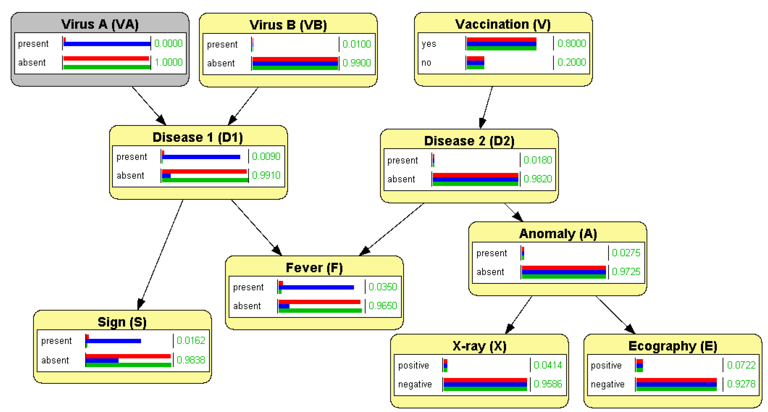
In OpenMarkov chance variables are drawn as rounded rectangles and colored in cream, as shown in Figure 1. When a finding is entered (usually by double-clicking on the value/state of the variable), OpenMarkov propagates it and shows the posterior probability by means of a horizontal bar. It is possible to have several sets of findings, each called an evidence case, and display several bars for each state. Figure 1 shows three evidence cases: in the first one, corresponding to the red bars, there is no finding (); in the second one, shown in blue, the presence of virus A is confirmed, so and ; in the third one, shown in green, this virus is known to be absent, i.e., and . This allows the user to see how the probabilities of the variables change when new findings are entered.
3.2. Correlation and Independence
3.2.1. Conditional Independence
Even though the concepts of probabilistic dependence (correlation) and independence are mathematically very simple (cf. Equation (1)), many students have difficulties to understand them intuitively, especially in the case of conditional independence. In our teaching, we use the network in Figure 1, which has a clear causal interpretation: all the variables are Boolean, and for each link , the finding +x increases the probability of +y, except in the case of vaccination, +v, which decreases the probability of being present.
In order to illustrate a priori independence, we point out that in this model there is no link between the two viruses, and , and they have no common ancestors. Therefore, they are d-separated in the graph, and because of Property (5) (with ), they are a priori independent. We can check it by introducing a finding for and observing that the probability of does not change, or vice versa; for example, , as shown in Figure 1, which confirms that Equation (2) holds. In contrast, we can see that the variables and are correlated by introducing evidence about the one and observing that the probability of the other changes; for example, in Figure 1 we observe that +|+.
We can also see that in this graph each node at the left of F is separated from each variable at its right when , which implies that they are pairwise a priori independent—see again Figure 1. We can verify it by introducing evidence for one variable in one side and observing that the probabilities on the other side do not change.
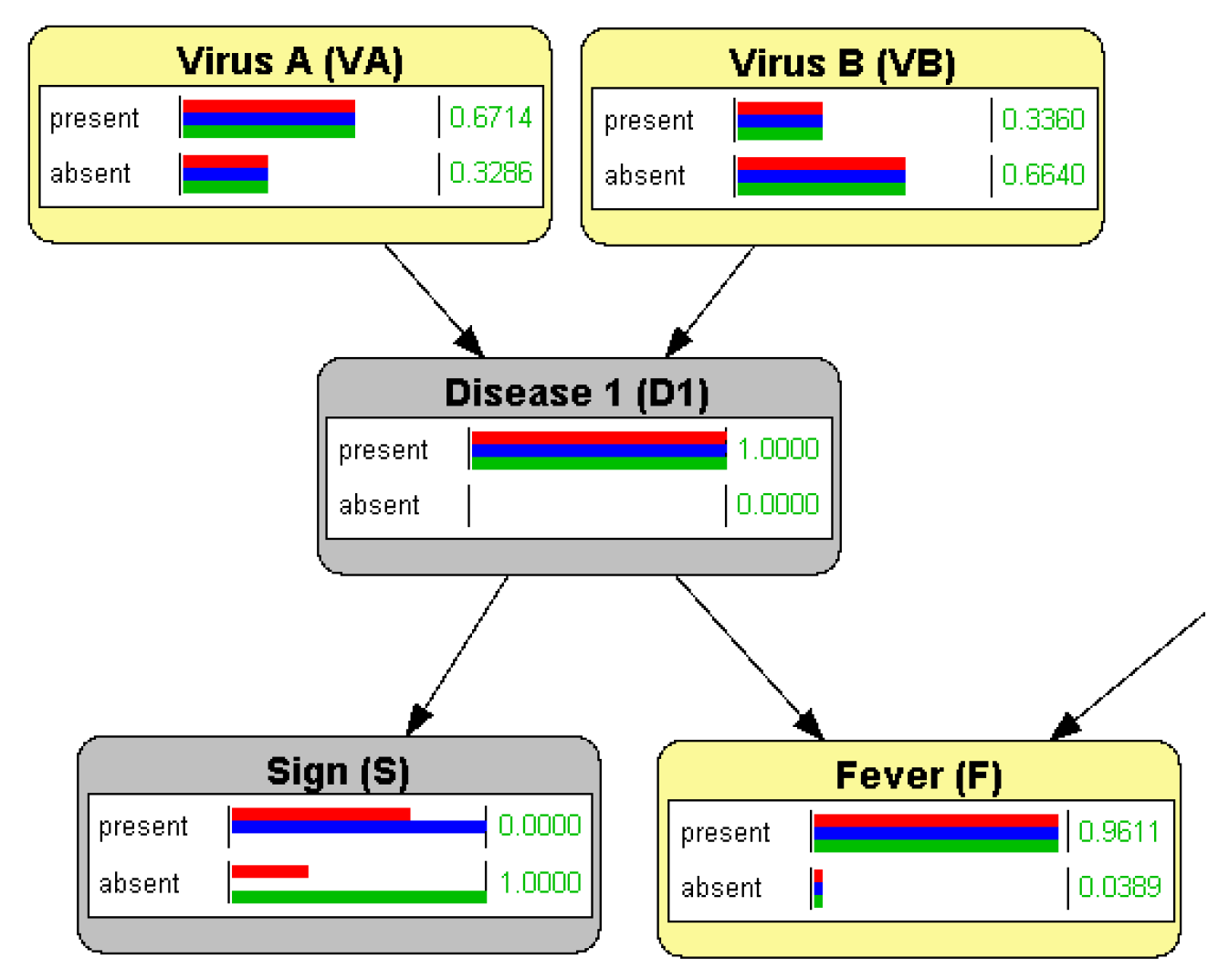
To illustrate conditional independence, we first show that S (a sign) and F (fever) are a priori correlated by introducing evidence on one of them and seeing that the probability of the other changes. However, if we first introduce evidence about , which plays the role of , and introduce a finding S (by generating a new evidence case in OpenMarkov), then the probability of F does not change, as we can observe in Figure 2. This shows that F and S, despite being correlated a priori, are conditionally independent given (it is an instance of Equation (1) with ). Our students easily understand that the correlation between fever and the sign is due to a common cause, and when we know with certainty whether this cause is present or absent, the correlation disappears. OpenMarkov confirms that our intuitive understanding of causation leads to the numerical results we expected.
3.2.2. d-Separation
Section 2.2.1 introduced the definition of d-separation. If we just left our students with it (or with its equivalent definition in Proposition 1), they would be absolutely unable to understand the rationale behind it—so would we! In particular, it is difficult to understand why some trails are active if and only if the intermediate node is in , while for other trails the opposite is true—see Definition 2. Additionally, a convergent path , which is a priori inactive, can be activated not only by Z but also by any of its descendants, while a divergent path , which is a priori active, can be blocked by X but not by its ancestors. It sounds arbitrary, if not esoteric.
To make d-separation intuitive, we explain that this property is a consequence of the factorization of the probability (cf. Equation (3)) and that it agrees with our notions of causality, provided that in Definition 2 is interpreted as the evidence, i.e., a set of findings for the observed variables. We first consider that a path containing just one link is always active, by definition, whatever the evidence. We can observe for the network in Figure 1 that introducing a finding for one variable affects the posterior probabilities of all its neighbors, even if there is evidence for other nodes. The correlation in this case is explained by a direct cause-effect relation.
We then consider a divergent trail, such as . Definition 2 says that this path is active a priori, i.e., when there is no evidence. We can verify it by introducing a finding for S or for F, as explained above. This correlation is intuitive because S and F are effects of a common cause. However, when the presence or the absence of this disease is confirmed or ruled out by direct observation, then , and implies . We can check it by first entering evidence for and then, in a new evidence case, adding a finding for S, either or ; the probability of F does not change, as shown in Figure 2. This also agrees with our notion of causal influence.
The behavior of a sequential trail is similar; for example, the path means that the causal influence of on S is mediated by . This path is active a priori because detecting virus A increases the probability of the disease and, consequently, that of the symptom (deductive reasoning). Similarly, the symptom makes us suspect the presence of the virus (abductive reasoning). However, the finding blocks this path, because once we know that the disease is present (or absent), the information about the virus does not affect the probability of the symptom, and vice versa. We can check it with OpenMarkov. Again, d-separation agrees with our intuitive notion of causality.
Let us now consider the convergent trail . When , it is inactive and and are separated. (At this point, it may be worth warning our students that, contrary to intuition, “being connected” is not a transitive property: is connected with and is connected with , but is not connected with . The analysis of whether a path is active cannot be done link by link, because an individual link is always active; it is necessary to consider every pair of consecutive links, i.e., every trail, as in Definition 2 and Proposition 1. The lesson is that, even though intuition is very useful in mathematics, it must be properly trained and supported by formal reasoning.)
We can check that and are separated—and, because of Property (5), a priori independent—by introducing evidence for and observing that the probability of does not change, as shown in Figure 1. This is intuitive, because there is no common cause for these variables. In contrast, when there is evidence about , the trail becomes active and, consequently, and are no longer separated: . We can verify it by first introducing evidence about —for example, —, generating a new evidence case, introducing evidence about , and observing that now the probability of changes: . This is consistent with the causal interpretation of the BN, because when a patient has the first disease, we suspect that the cause is virus A or virus B; if additional evidence (for example, the result of a test) leads us to ruling out virus A, we then suspect that the cause of the disease is virus B; conversely, if the presence of A is confirmed, our suspicion of B decreases. Put another way, the finding + creates a negative correlation between and , which were are a priori independent. This phenomenon, called explaining away [5], is the most typical case of intercausal reasoning; in particular, it is a property of the noisy-OR model [5,26]. (In this network there is another noisy OR at F.)
It also follows from the definition of d-separation that the convergent trail is not only activated by itself, but also by any of its descendants. We can verify it with OpenMarkov by introducing the findings +s or +f. This is another instance of explaining-away because any of these findings makes us suspect the presence of at least one of the viruses, with a negative correlation between and .
We may now ask ourselves: if the middle node in a divergent trail can block it, and the descendants of the middle node can activate a convergent trail, why cannot the ancestors of the middle node in a divergent trail block it? We can check with OpenMarkov that this is the case; for example, given the trail , if we first introduce the finding and then add in a new evidence case the finding , we observe that the probability increases, which proves that S and F are not conditionally independent given . The reason for this correlation is that the presence of a virus increases the probability of the disease, but—unlike the case in which the disease is confirmed by direct observation—the probability is not yet 100%, so it can be further increased by . We can also try other combinations of findings to check that no ancestor of blocks this trail.
3.2.3. Markov Property and Markov Blankets
As we saw in Section 2.2.1 (cf. Equation (4)), the Markov property means that every node is conditionally independent of its non-descendants given its parents. Again, this definition may be difficult to understand for students when stated in abstract, but it is intuitive when explained with examples. In particular, when a node has no parents, it is conditionally independent of its non-descendants. We can illustrate it with the two-diseases network (Figure 1) by showing, for example, that the probability of Disease 1 does not change when introducing evidence for the nodes at the right of Fever, which are not descendants of that disease; and vice versa. Similarly, we can introduce evidence for the parents of a node—for example, Fever—and then see that adding evidence about other nodes that are not its descendants does not alter its probability.
We can illustrate in the same manner the concept of Markov blanket, which denotes a set of nodes that surround a node, making it conditionally independent of the other variables in the network [5]. One might think that the set of parents and children of a node constitute a Markov blanket for it. However, this is not the case: if we introduce evidence for the parents and children of , i.e., for , S, and F, we can see that is not yet separated from all the other nodes in the network; in fact, every node in is correlated with because F has activated the trail . Therefore, the Markov blanket of a node must include not only its parents and children, but also the parents of its children.
3.3. Inference Algorithms for Bayesian Networks
We have seen that OpenMarkov is able to propagate evidence, but so far we have not discussed inference algorithms. In this section, we explain how this tool can help illustrate some of the basic algorithms, namely, arc reversal, logic sampling, and likelihood weighting.
3.3.1. Arc Reversal for Bayesian Networks
Arc reversal was initially designed to transform IDs into decision trees [2], but in our opinion, students understand it better if it is first introduced for BNs.
Let us use again the two-diseases network (Figure 1) as an example. When processing the query , is the variable of interest and F, S, and V are the evidence variables. Then X and U can be removed in OpenMarkov’s GUI because they are barren nodes. Then A becomes a barren node, which can also be removed. The user can invert link by right-clicking on it; OpenMarkov replaces it with , adds a new link (because A was a parent of ), and computes the new probability table ; the probability does not change because A has received no new parent. Now B is barren and can be removed. The user can then invert to remove A. After inverting , which adds the links and , it is possible to remove . In each step the user can inspect the new CPTs and check that they have been computed correctly. Finally, after inverting and the parents of (the variable of interest) are the three evidence nodes, and the user can retrieve the probability by opening the CPT for .
When there is a link and another directed path from X to Y, the option for inverting the link is disabled in its contextual menu (it appears in gray) because it would create a cycle. In the future, we might add a dialog that would suggest to the user the node deletions and arc reversals that will lead to calculating the probability of the variable of interest.
3.3.2. Stochastic Algorithms
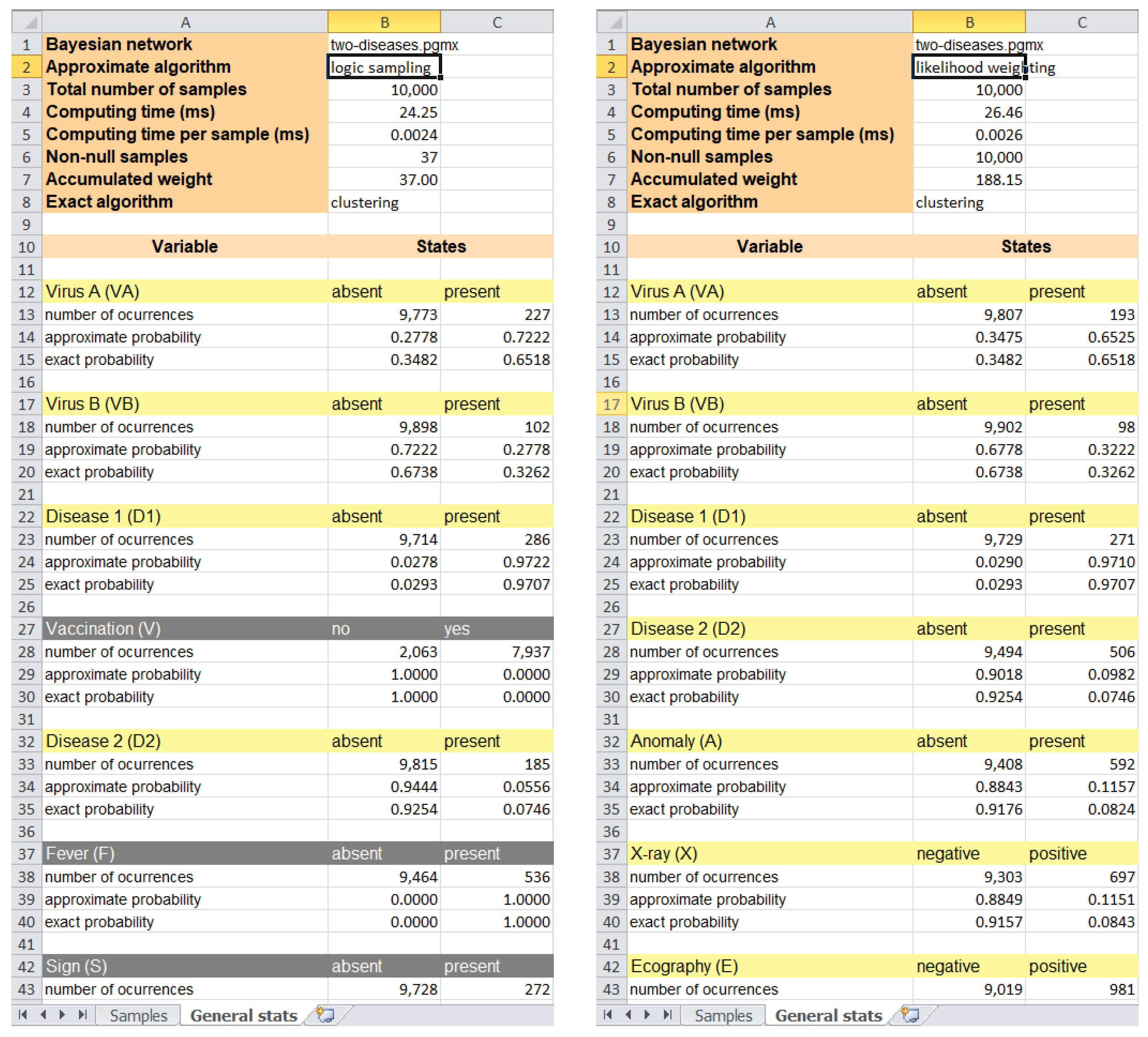
OpenMarkov currently implements two stochastic algorithms: logic sampling [27] and likelihood weighting [28]. Both start by sampling a value for each node without parents, using its prior distribution, and then proceed in topological order (i.e., downwards), sampling each other node in accordance with the probability distribution for the configuration of its parents. This way, every iteration of the algorithm obtains a sample—a configuration of all the nodes. OpenMarkov is able to store these configurations in a spreadsheet and compute some statistics, including the posterior probability of each variable, as shown in Figure 3.
The left side of this figure displays the output of the logic sampling algorithm. The 10,000 configurations obtained are stored in the “Samples” sheet (not visible in the figure), with a sample per row and a variable per column; those compatible with the evidence are colored in green and those incompatible in red. The “General stats” tab shows that only 37 samples are compatible (see cell B6), a clear indication of the inefficiency of this algorithm.
For each variable, the spreadsheet displays the number of samples in which each state has appeared; for example, has taken the state “absent” in 9714 samples (cell B23) and “present” in 286 (cell C23). It also shows the posterior probability for each state, which is not proportional to the number of occurrences because the samples incompatible with the evidence do not count.
The right side of Figure 3 shows the output of likelihood weighting. One difference with the previous algorithm is that it only samples the variables that do not make part of the evidence; therefore, the evidence variables are not shown in the sheet. Another difference is that now the number of non-null samples (cell B6) equals the number of samples, because all of them are valid. However, each sample has a weight between 0 and 1 (in logic sampling it was either 0 or 1), as shown in the “Samples” sheet. As a consequence, the total weight for this simulation is 188.15 (cell B6), much higher than the value of 37 obtained for logic sampling, and this usually leads to more accurate estimates of the posterior probabilities, as we can see by comparing the approximate probabilities with their exact probabilities for both algorithms.
3.4. Learning Bayesian Networks
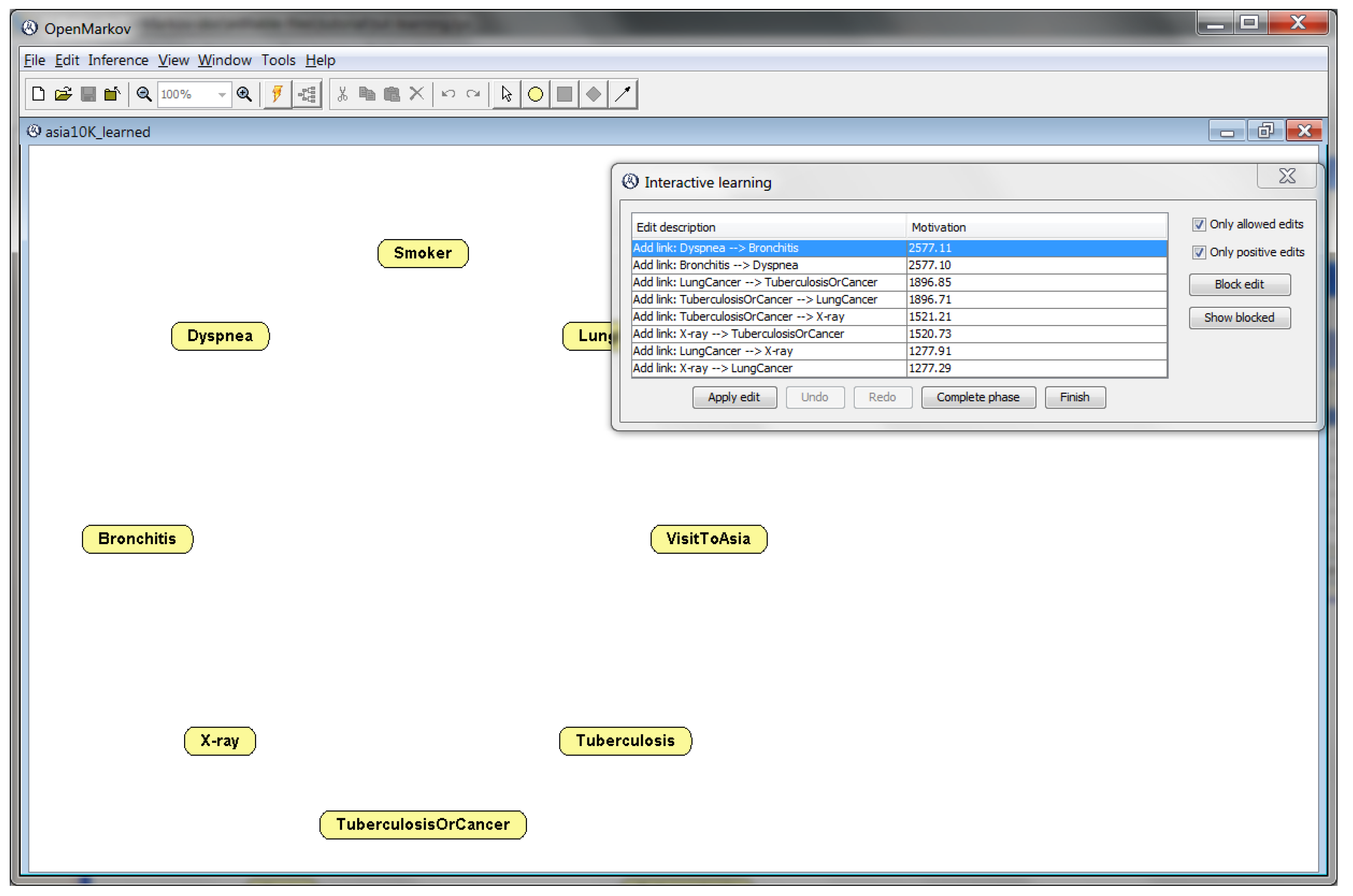
BNs can be built from human knowledge, data, or a combination of both. OpenMarkov implements the two basic algorithms for learning BNs from data: search-and-score [29] and PC [30]. Other tools offer many more algorithms, but the advantage of OpenMarkov is the possibility of interactive learning [31]: in every step, the GUI displays a list of the edits (operations) that it is ready to perform and a motivation for each edit, as shown in Figure 4 and Figure 5. This way, the user can monitor how the algorithm proceeds, step by step, and either accept the next edit proposed by the algorithm, or select another one from the list, or do a different edit at the GUI.
The search-and-score algorithm, also called “hill climbing”, departs from a network with a node for each variable in the data, and no link (cf. Figure 4). The possible edits are: adding a directed link (the most common edit), deleting one of the existing links, or inverting a link. This process is guided by a metric chosen by the user. Currently OpenMarkov offers six well-known metrics: BD, Bayesian, K2, entropy, AIC, and MDLM. When learning the network, it selects the edits compatible with the restrictions of the network (for example, a BN cannot have cycles) and ranks them according to their scores. This way, a student can see, for example, that when the network has no link yet, the K2 metric usually assigns different scores to the links and , although the resulting networks represent exactly the same probability distribution, which is an unsatisfactory property of this metric. It is also possible to see that every edit (for example, adding a link) usually changes the scores of future edits.
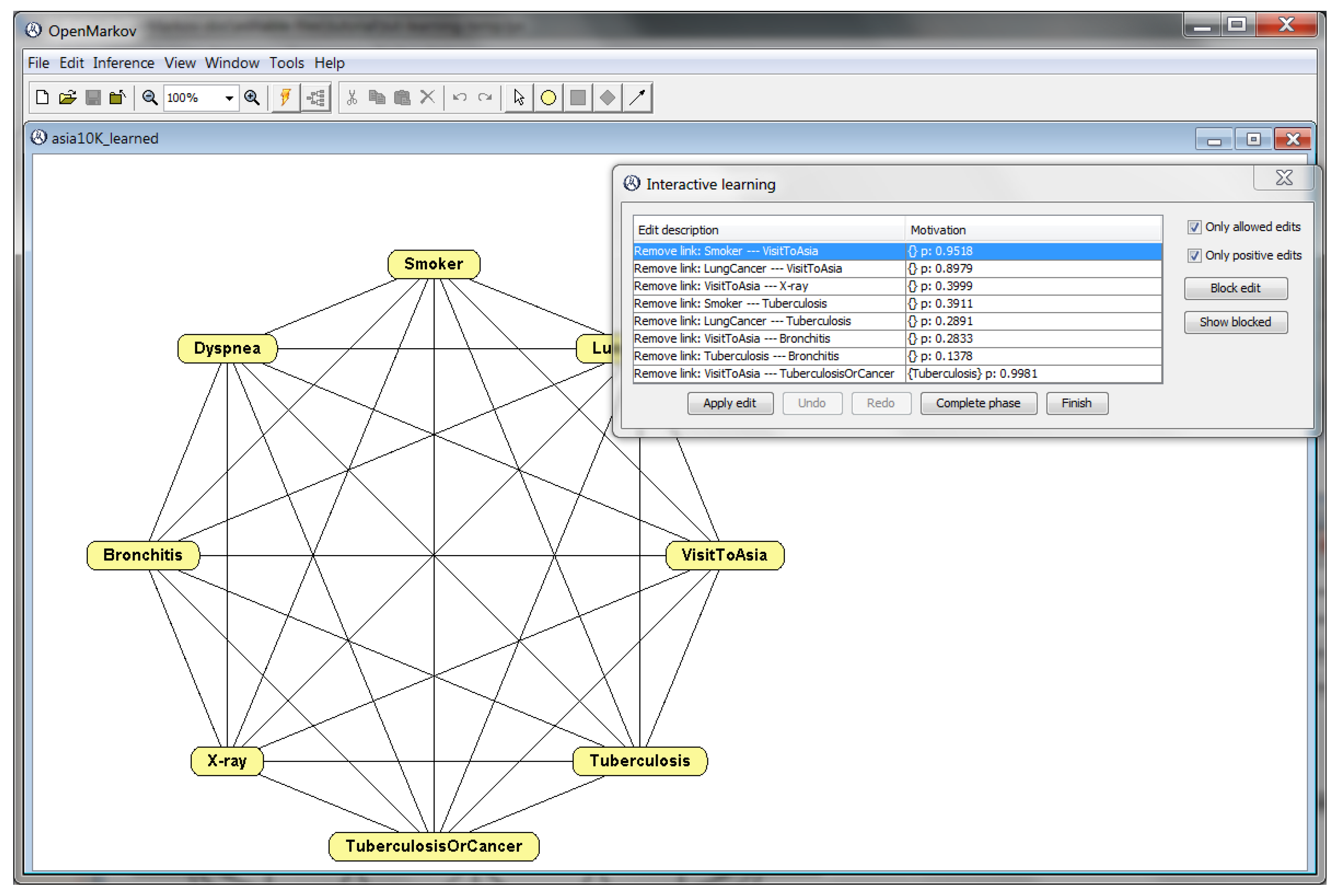
In contrast, the PC algorithm departs from a fully connected undirected graph (Figure 5) and removes the links one by one depending on the conditional independencies found in the database. For each undirected link X–Y, OpenMarkov performs a statistical test that returns the p-value for the “null hypothesis” that X and Y are a priori independent; if p is below a certain threshold, —called significance level, set by the user—, the null hypothesis is rejected and the link is kept; otherwise, it is removed. Links with higher p-values, which correspond to correlations that can be explained by chance, are proposed to be removed first. Then the PC algorithm tests, for each pair of variables, whether they are independent given a third variable, and then given a pair of other variables, and so on. In each step, the GUI shows the user a list of the links that might be removed, and for each link, the conditioning variables and the p-value. This way, the user can not only see the removals that the algorithm is considering, but also the certainty for each one. Finally, the algorithm assigns a direction to each link.
The tutorial of OpenMarkov, available at www.openmarkov.org/docs/tutorial; accessed on 20 September 2022, explains in detail the options it offers for learning BNs, either automatically or interactively.
4. Teaching Influence Diagrams
4.1. Evaluation of Influence Diagrams
4.1.1. Expected Utility and Optimal Policies
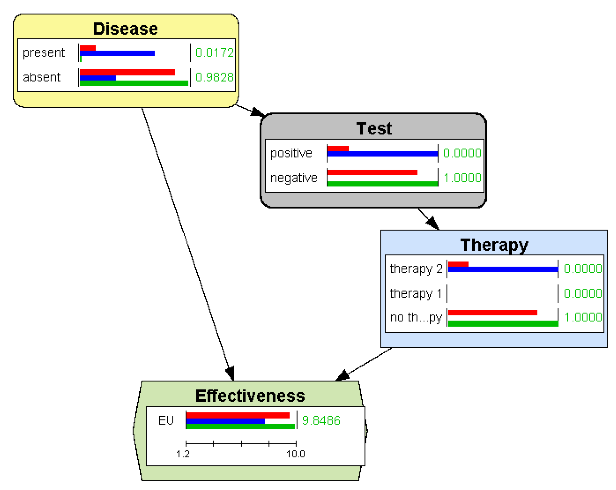
In Section 2.2.2 we mentioned that the evaluation of an ID consists in finding the maximum expected utility (MEU) and an optimal strategy. When OpenMarkov evaluates an ID in the GUI, it presents to the user the posterior probability of each chance and decision node and the expected utility of each utility node, as shown in Figure 6.
One way to evaluate an ID—the original method proposed by Howard and Matheson [2] when introducing this formalism—is to convert it into an equivalent decision tree (DT). For example, the ID in Figure 6 can be expanded into the DT in Figure 7, where each branch is labeled with its expected utility, obtained when evaluating the tree from the leaves to the root; for every decision node, one of its branches is marked with a small red rectangle to indicate the optimal choice in that scenario (in the case of a tie, more than one branch would have this mark). This evaluation method is very inefficient, because the size of the tree grows exponentially with the number of nodes in the ID. In fact, in our group we have built IDs for some medical problems [32,33], having fewer than 30 nodes, whose equivalent DTs contain tens of thousands of leaves. However, when teaching PGMs it is very useful to compare IDs with DTs for small problems because, in our opinion, an ID can only be understood as a compact representation of a DT, and all the algorithms for evaluating IDs take the DT as a reference. For these reasons, we implemented in OpenMarkov the automatic conversion of IDs into DTs.
However, OpenMarkov can also evaluate IDs with more efficient algorithms; by default, the GUI uses variable elimination [9,34]. After the evaluation, in addition to showing the posterior probability of each chance variable, with a bar for each evidence case, as in the case of BNs, it also displays a bar for every state (option) of every decision and for the expected utility of every utility node. For example, Figure 6 displays the probabilities and the expected utility for three evidence cases: when the test is not yet done (red bars), when it is positive (blue bars), and when it is negative (green bars).
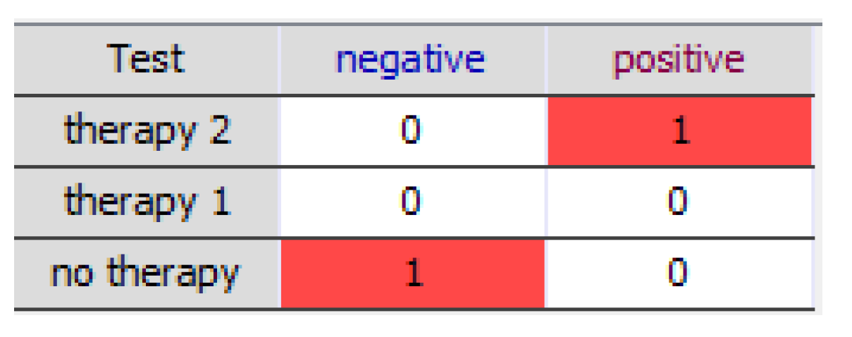
The optimal strategy calculated by OpenMarkov can be examined in different ways. One of them is to open for each decision D the probability table for the optimal policy—cf. Section 2.2.2. Since the optimal policies are deterministic—except in the case of ties—these tables usually contain only 0’s and 1’s, as in Figure 8, where the only informational predecessor of the decision (the only variable known when making it) is the result of the test.
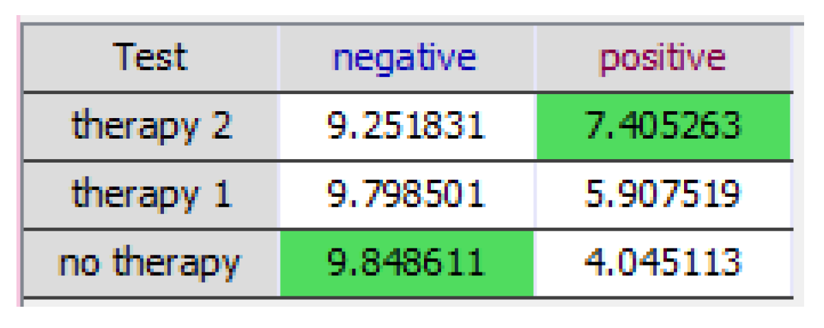
More insight about this policy is presented in Figure 9, which shows the expected utilities obtained when calculating the optimal policy for Therapy—cf. Equation (10).
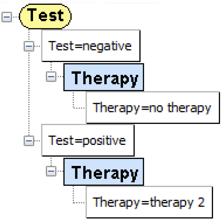
An alternative way to see the optimal strategy in OpenMarkov is to display the strategy tree [35], which summarizes all the policies in one figure. It is more compact than the DT—please compare Figure 7 and Figure 10—because it prunes the suboptimal branches (which implies that only one branch goes out from each decision node, except in the case of a tie) as well as the branches with null probability (for example, when we decide not to do a test, its result is neither “positive” nor “negative”). The strategy tree is very useful for large IDs; for example, the optimal-policy table for the last decision in Mediastinet, an ID for lung cancer [32], contained more than 15,000 columns, but only 5 were relevant because the others corresponded to impossible or suboptimal scenarios. In contrast, the strategy for that ID only has 5 leaves, one for each relevant column [35].
4.1.2. Arc Reversal for Influence Diagrams
As mentioned above, arc reversal was introduced by Howard and Matheson [2] to transform IDs and convert them into DTs. Later, Olmsted [12] designed an algorithm that iteratively removes the nodes from the graph, one by one, until only the utility node remains; this is much more efficient than expanding a DT—see also [13].
Again, we can illustrate this algorithm with OpenMarkov. For example, when evaluating the ID in Figure 6, we should remove first the node Disease because it is not an informational predecessor of any decision; but this node has a descendant that is not a utility node. We can then invert the link Disease → Test by right-clicking on it, as in BNs. Now Effectiveness, a utility node, is the only descendant of Disease, so the user can click “Absorb node” on the contextual menu of this node, which adds a link from Test to Effectiveness and computes the new utility table with Equation (11). If Disease were the parent of more than one utility node, OpenMarkov would fuse them into a single node, as explained in Section 2.2.3. Then the only descendant of Therapy is the utility node, and this decision can be absorbed by applying Equation (12); the optimal policy is obtained from Equation (10). Now the only descendant of Test is the utility node, so this chance node can be absorbed by applying again Equation (11). At the end, only one utility node remains in the ID; its potential contains a single numerical parameter, which is the MEU.
4.1.3. Expected Value of Perfect Information (EVPI)
A relevant concept in decision analysis is the EVPI [36], which measures the advantage we would obtain from a certain piece of information, such as knowing the exact value of a parameter or the value taken by a variable. For example, given the ID in Figure 6, we may ask ourselves: “What would be the value of knowing for sure whether the patient has the disease (or not) before deciding about the therapy?” In OpenMarkov this question can be easily solved by drawing an information link from Disease to Therapy. Students can observe that the expected utility (effectiveness) increases from 9.3937—see Figure 6—to 9.5100, which means that the EVPI is 0.1163. This example illustrates the advantages of IDs, because if the original problem had been modeled with a decision tree, computing the EVPI would require building a new decision tree almost from scratch.
4.2. Explanation of Reasoning
OpenMarkov offers several options for explaining the conclusions achieved by an ID, most of them developed for its predecessor, Elvira [24]. These options have been useful for our research group when building BNs and IDs for medicine [23] and also for teaching PGMs to our students.
4.2.1. Imposing Policies for What-If Reasoning
OpenMarkov allows the user to impose policies on some decision nodes, in which case the evaluation algorithm only calculates optimal policies for the other decisions, which may differ from those obtained without imposed policies. This functionality allows the user to analyze decision scenarios that can never occur if the decision maker applies the optimal strategy, thus performing what-if reasoning [24].
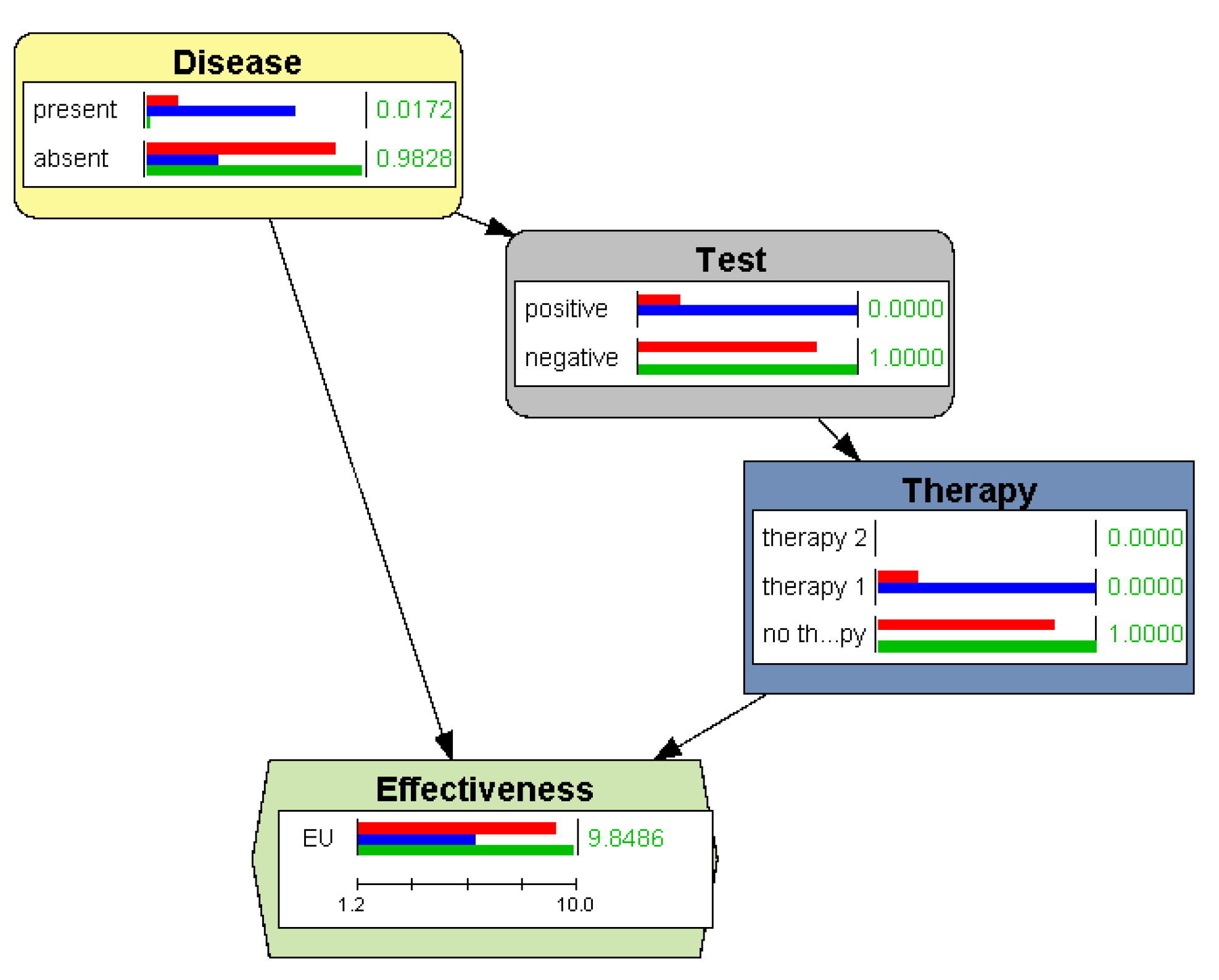
For example, the optimal strategy for the ID in Figure 6 is: “if the result of test is negative, then do not apply any therapy; otherwise, apply therapy 2”. However, the user might wish to investigate other policies, such as applying therapy 1 instead of therapy 2 when the test is positive, or applying therapy 1 in all cases, and calculate the expected utility for different results of the test, as shown in Figure 11.
4.2.2. Introducing Evidence
Lacave et al. [24] distinguished two types of evidence in the context of IDs: pre-resolution and post-resolution. Post-resolution evidence is introduced when every decision has been assigned a policy, either by the user or by the evaluation algorithm. The goal is to see how some findings affect the posterior probabilities—as in BNs—and the expected utilities. We have already seen two examples in Figure 6 and Figure 11: OpenMarkov displays the utility expected before doing the test (which is the same as the utility for the general population, because some people test positive and others test negative), but we can also compute the expected utility and the posterior probability of the disease for those people having a positive test result and for those having a negative result.
In contrast, pre-resolution evidence corresponds to the classical definition of evidence in IDs [37]. In this case the question is: “What would the optimal strategy and the expected utilities be if we had that information when making the decisions?”
4.2.3. Example: Justifying a Policy
The usefulness of these two explanation facilities can be illustrated with the following example, adapted from a situation we encountered during the construction of an ID for lung cancer [32], when the pneumologist did not understand why the model built so far advised against doing a test that, in his opinion, would be useful.
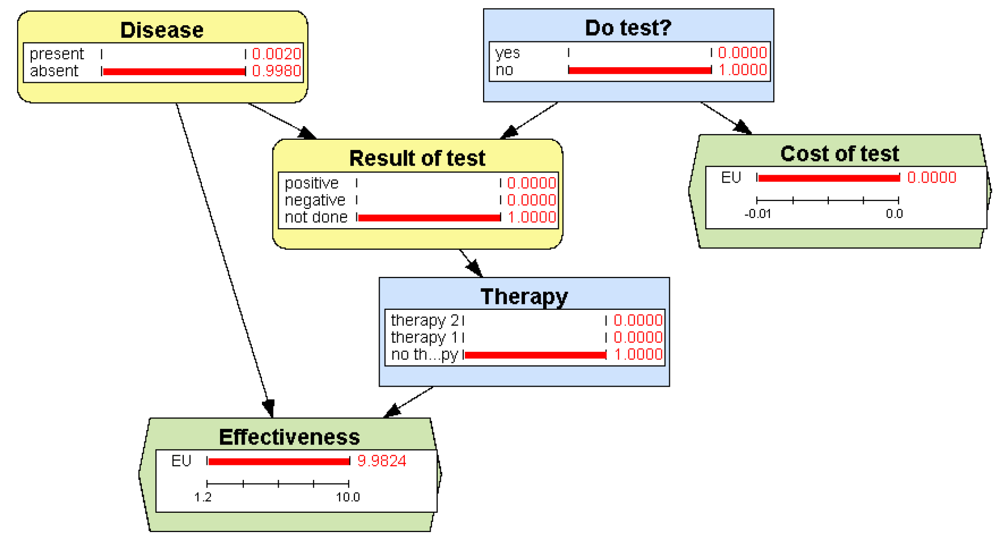
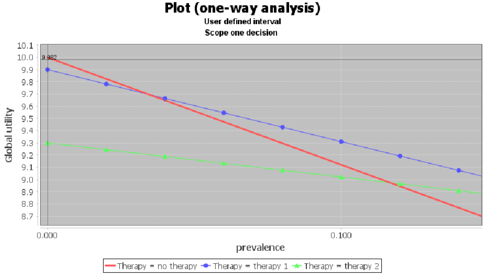
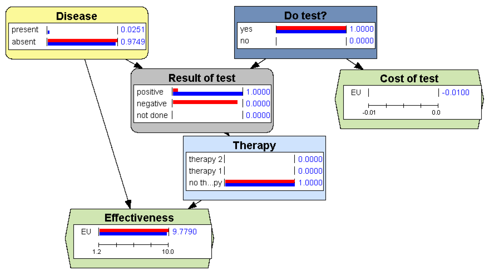
The ID in Figure 12 presents a similar situation, in which it is better not doing the test, which might be counterintuitive. The reason seems to be that the result of the test does not modify the optimal policy. To confirm it, we first perform the sensitivity analysis shown in Figure 13, which shows that when the probability of disease is below 3.45% no therapy should be applied. Then we try to find out the posterior probability of disease after a positive test, but when we try to introduce the finding “Result of test = positive”. OpenMarkov throws an error message saying that this finding is incompatible with the optimal policy, which precludes doing the test. A workaround consists in imposing the policy “Do test? = yes”, which allows us introducing that finding and observing that the posterior probability increases of disease increases only to 2.51% (see Figure 14), still below the 3.45% threshold.
5. Discussion and Conclusions
OpenMarkov is an open-source tool for building and evaluating several types of PGMs. It has been especially designed for medical applications and for teaching. It has been used for research and tuition in more than 30 countries.
In this paper we have illustrated with several examples how to teach several aspects of PGMs with OpenMarkov. Some of them—for example, the properties of d-separation, which are far from intuitive for beginners—might be illustrated with any other tool having a graphical user interface (GUI) able to show on a screen the graph of the model and a probability bar for each node, such as those mentioned in Section 2.3, but the explanation is much clearer if there is a probability bar for each evidence case, a feature that is only available in OpenMarkov. This tool also allows building networks in which some conditional probability tables (CPTs) are encoded as canonical models based on the independence of causal interactions, such as the noisy and leaky of the OR, AND, MAX, MIN, etc. [5,26], and implements efficient algorithms for evaluating them [38]. Students can learn how to apply these models and how they behave when propagating evidence.
Additionally OpenMarkov is useful to illustrate the execution of several iterative algorithms for inference and learning. In particular, it is able to display on a spreadsheet the samples generated by stochastic algorithms, as well the number of valid samples, the accumulated weights, and the posterior probabilities. It also allows the user to apply arc reversal iteratively for both BNs and IDs, showing how the probabilities and the utility tables are updated in each step. Similarly, it can learn BNs from a database using several variations of the two basic algorithms, search-and-score (hill climbing) and PC; in this case, the GUI offers several edits (such as adding, removing, or inverting a link), along with a qualitative score for each one, so that the user can understand what the algorithm intends to do and why. Students can compare the performance of different algorithms by observing not only the differences in the networks learned from the same database, but also how the algorithms differ step by step.
Our tool offers several possibilities for evaluating IDs. One of them is the conversion into decision trees, which can only be done for very small problems, but is very useful to intuitively understand the relation between the two formalisms. OpenMarkov can also apply efficient algorithms, such as variable elimination and arc reversal, and show the optimal policy (a table) for each decision, as well as the expected utility and the posterior probability of each chance and decision node, with the possibility of entering pre- and post-resolution evidence to observe how those utilities and probabilities vary. It can also show the optimal strategy in the form of a tree (cf. Figure 10), which is much more compact than the decision tree and the policy tables. Most of these features are not available in any other tool, whether commercial, free, or open-source.
Finally, OpenMarkov has novel types of PGMs, such as Markov influence diagrams [14] and decision analysis networks [15], developed by our research group, as well as new algorithms for cost-effectiveness analysis with these models [14,39,40]. They can be very useful for teaching health technology assessment (HTA), but that topic is out of the scope of this paper.
A limitation of OpenMarkov is that, although it implements several algorithms for exact inference, it only offers the most basic algorithms for stochastic inference and for learning. We implemented them just for pedagogical purposes, because these topics fall outside the priorities of our research group.
However, being open-source is an important advantage of OpenMarkov because it allows students with some knowledge of Java to inspect the implementation of the algorithms. For example, in the abstract class StochasticPropagation.java the students can find the data structures and methods common to the two algorithms discussed in this paper, while the classes that extend it, namely, LogicSampling.java and LikelihoodWeighting.java, implement the aspects in which the algorithms differ. Furthermore, advanced students can add new features—see [41] as an example. In fact, a significant part of OpenMarkov’s code has been written by undergraduate, master, and Ph.D. students. In the future, other researchers and students, not necessarily from our university, might contribute new algorithms for inference and learning. This tool can be especially useful as a workbench for new learning algorithms because it has been carefully designed to allow implementing other algorithms, integrating them in the GUI, and executing them interactively.
Given that nowadays PGMs make part of the computer science curriculum in all universities around the world, we hope that many teachers and students may consider using OpenMarkov as a pedagogical tool, and some of them will later use it for building real-world applications.
Author Contributions
M.A. implemented Carmen, the first prototype of this software tool. All authors have contributed to the design and implementation of OpenMarkov, and to writing, reviewing, and editing the manuscript. All authors have read and agreed to the published version of the manuscript.
Funding
This work has been supported by grant PID2019-110686RB-I00 from the Spanish Government. The development of OpenMarkov has also received support from other grants of the Spanish Government and from the Regional Government of Madrid, most of them co-financed by the European Regional Development Fund.
Data Availability Statement
Some of the networks shown in this paper, together with several PMGs for real-world medical problems, are available at http://www.probmodelxml.org/networks; accessed on 20 September 2022.)
Acknowledgments
We thank the reviewers of this journal and those of the PGM-2018 conference for their comments and corrections. We thank all the students who have collaborated in the development of OpenMarkov, in particular, José Enrique Mendoza and Antonio Sáez for their work on the GUI, and Iago París for implementing arc reversal and the stochastic algorithms.
Conflicts of Interest
The authors declare no conflict of interest.
Abbreviations
The following abbreviations are used in this manuscript:
| BN | Bayesian network |
| CPT | Conditional probability table |
| DT | Decision tree |
| GUI | Graphical user interface |
| ID | Influence diagram |
| MEU | Maximum expected utility |
| PGM | Probabilistic graphical model |
References
- Pearl, J. Fusion, propagation and structuring in belief networks. Artif. Intell. 1986, 29, 241–288. [Google Scholar] [CrossRef]
- Howard, R.A.; Matheson, J.E. Influence diagrams. In Readings on the Principles and Applications of Decision Analysis; Howard, R.A., Matheson, J.E., Eds.; Strategic Decisions Group: Menlo Park, CA, USA, 1984; pp. 719–762. [Google Scholar]
- Howard, R.A.; Matheson, J.E. Influence diagrams. Decis. Anal. 2005, 2, 127–143. [Google Scholar] [CrossRef]
- Pearl, J. Probabilistic Reasoning in Intelligent Systems: Networks of Plausible Inference; Morgan Kaufmann: San Mateo, CA, USA, 1988. [Google Scholar]
- Koller, D.; Friedman, N. Probabilistic Graphical Models: Principles and Techniques; The MIT Press: Cambridge, MA, USA, 2009. [Google Scholar]
- Sucar, L.E. Probabilistic Graphical Models. Principles and Applications; Springer: London, UK, 2015. [Google Scholar]
- Díez, F.J.; París, I.; Pérez-Martín, J.; Arias, M. Teaching Bayesian networks with OpenMarkov. In Proceedings of the Ninth European Workshop on Probabilistic Graphical Models (PGM’18), Prague, Czech Republic, 11–14 September 2018. [Google Scholar]
- Neapolitan, R.E. Probabilistic Reasoning in Expert Systems: Theory and Algorithms; Wiley-Interscience: New York, NY, USA, 1990. [Google Scholar]
- Luque, M.; Díez, F.J. Variable elimination for influence diagrams with super-value nodes. Int. J. Approx. Reason. 2010, 51, 615–631. [Google Scholar] [CrossRef]
- Nielsen, T.D.; Jensen, F.V. Welldefined decision scenarios. In Proceedings of the Fifteenth Conference on Uncertainty in Artificial Intelligence (UAI’99), Stockholm, Sweden, 30 July–1 August 1999; Laskey, K., Prade, H., Eds.; Morgan Kaufmann: San Francisco, CA, USA, 1999; pp. 502–511. [Google Scholar]
- Cowell, R.G.; Dawid, A.P.; Lauritzen, S.L.; Spiegelhalter, D.J. Probabilistic Networks and Expert Systems; Springer: New York, NY, USA, 1999. [Google Scholar]
- Olmsted, S.M. On Representing and Solving Decision Problems. Ph.D. Thesis, Dept. Engineering-Economic Systems, Stanford University, Stanford, CA, USA, 1983. [Google Scholar]
- Shachter, R.D. Evaluating influence diagrams. Oper. Res. 1986, 34, 871–882. [Google Scholar] [CrossRef]
- Díez, F.J.; Yebra, M.; Bermejo, I.; Palacios-Alonso, M.A.; Arias, M.; Luque, M.; Pérez-Martín, J. Markov influence diagrams: A graphical tool for cost-effectiveness analysis. Med. Decis. Mak. 2017, 37, 183–195. [Google Scholar] [CrossRef] [PubMed]
- Díez, F.J.; Luque, M.; Bermejo, I. Decision analysis networks. Int. J. Approx. Reason. 2018, 96, 1–17. [Google Scholar] [CrossRef]
- Lauritzen, S.L.; Nilsson, D. Representing and solving decision problems with limited information. Manag. Sci. 2001, 47, 1235–1251. [Google Scholar] [CrossRef]
- Dean, T.; Kanazawa, K. A model for reasoning about persistence and causation. Comput. Intell. 1989, 5, 142–150. [Google Scholar] [CrossRef]
- Boutilier, C.; Dearden, R.; Goldszmidt, M. Stochastic dynamic programming with factored representations. Artif. Intell. 2000, 121, 49–107. [Google Scholar] [CrossRef]
- Boutilier, C.; Poole, D. Computing optimal policies for partially observable decision processes using compact representations. In Proceedings of the Thirteenth National Conference on Artificial Intelligence (AAAI’96), Portland, OR, USA, 4–8 August 1996; Clancey, W.J., Weld, D.S., Eds.; AAAI Press/MIT Press: Portland, OR, USA, 1996; pp. 1168–1175. [Google Scholar]
- Díez, F.J.; van Gerven, M.A.J. Dynamic LIMIDs. In Decision Theory Models for Applications in Artificial Intelligence: Concepts and Solutions; Sucar, L.E., Hoey, J., Morales, E., Eds.; IGI Global: Hershey, PA, USA, 2011; pp. 164–189. [Google Scholar]
- Elvira Consortium. Elvira: An environment for creating and using probabilistic graphical models. In Proceedings of the First European Workshop on Probabilistic Graphical Models (PGM’02). In In Proceedings of the First European Workshop on Probabilistic Graphical Models (PGM’02), Cuenca, Spain, 6–8 November 2002; pp. 1–11. [Google Scholar]
- Oliehoek, F.A.; Spaan, M.T.J.; Terwijn, B.; Robbel, P.; Messias, J.V. The MADP Toolbox: An open source library for planning and learning in (multi-)agent systems. J. Mach. Learn. Res. 2017, 18, 1–5. [Google Scholar]
- Lacave, C.; Oniśko, A.; Díez, F.J. Use of Elvira’s explanation facilities for debugging probabilistic expert systems. Knowl.-Based Syst. 2006, 19, 730–738. [Google Scholar] [CrossRef]
- Lacave, C.; Luque, M.; Díez, F.J. Explanation of Bayesian networks and influence diagrams in Elvira. IEEE Trans. Syst. Man Cybern.—Part B Cybern. 2007, 37, 952–965. [Google Scholar] [CrossRef] [PubMed]
- Teach, R.L.; Shortliffe, E.H. An analysis of physician’s attitudes. In Rule-Based Expert Systems: The MYCIN Experiments of the Stanford Heuristic Programming Project; Addison-Wesley: Reading, MA, USA, 1984; pp. 635–652. [Google Scholar]
- Díez, F.J.; Druzdzel, M.J. Canonical Probabilistic Models for Knowledge Engineering; Technical Report CISIAD-06-01; UNED: Madrid, Spain, 2006. [Google Scholar]
- Henrion, M. Propagation of uncertainty by logic sampling in Bayes’ networks. In Proceedings of the Uncertainty in Artificial Intelligence 4 (UAI’88), Minneapolis, MN, USA, 10–12 July 1988; Shachter, R.D., Levitt, T., Kanal, L.N., Lemmer, J.F., Eds.; Elsevier Science Publishers: Amsterdam, The Netherlands, 1988; pp. 149–164. [Google Scholar]
- Fung, R.; Chang, K.C. Weighing and integrating evidence for stochastic simulation in Bayesian networks. In Proceedings of the Uncertainty in Artificial Intelligence 6 (UAI’90), Cambridge, MA, USA, 27–29 July 1990; Bonissone, P., Henrion, M., Kanal, L.N., Lemmer, J.F., Eds.; Elsevier Science Publishers: Amsterdam, The Netherlands, 1990; pp. 209–219. [Google Scholar]
- Cooper, G.F.; Herskovits, E. A Bayesian method for the induction of probabilistic networks from data. Mach. Learn. 1992, 9, 309–347. [Google Scholar] [CrossRef]
- Spirtes, P.; Glymour, C. An algorithm for fast recovery of sparse causal graphs. Soc. Sci. Comput. Rev. 1991, 9, 62–72. [Google Scholar] [CrossRef]
- Bermejo, I.; Oliva, J.; Díez, F.J.; Arias, M. Interactive learning of Bayesian networks with OpenMarkov. In Proceedings of the Sixth European Workshop on Probabilistic Graphical Models (PGM’12), Granada, Spain, 19–21 September 2012; pp. 27–34. [Google Scholar]
- Luque, M.; Díez, F.J.; Disdier, C. Optimal sequence of tests for the mediastinal staging of non-small cell lung cancer. BMC Med. Inform. Decis. Mak. 2016, 16, 9. [Google Scholar] [CrossRef] [PubMed]
- León, D. A Probabilistic Graphical Model for Total Knee Arthroplasty. Master’s Thesis, Department Artificial Intelligence, UNED, Madrid, Spain, 2011. [Google Scholar]
- Jensen, F.V.; Nielsen, T.D. Bayesian Networks and Decision Graphs, 2nd ed.; Springer: New York, NY, USA, 2007. [Google Scholar]
- Luque, M.; Arias, M.; Díez, F.J. Synthesis of strategies in influence diagrams. In Proceedings of the Thirty-third Conference on Uncertainty in Artificial Intelligence (UAI’17), Sydney, Australia, 11–15 August 2017; AUAI Press: Corvallis, OR, USA, 2017; pp. 1–9. [Google Scholar]
- Felli, J.C.; Hazen, G.B. Sensitivity Analysis and the Expected Value of Perfect Information. Med. Decis. Mak. 1998, 18, 95–109. [Google Scholar] [CrossRef] [PubMed]
- Ezawa, K.J. Value of evidence on influence diagrams. In Proceedings of the Tenth Conference on Uncertainty in Artificial Intelligence (UAI’94), Seattle, WA, USA, 29–31 July 1994; de Mántaras, R.L., Poole, D., Eds.; Morgan Kaufmann: San Francisco, CA, USA, 1994; pp. 212–220. [Google Scholar]
- Díez, F.J.; Galán, S.F. Efficient computation for the noisy MAX. Int. J. Intell. Syst. 2003, 18, 165–177. [Google Scholar] [CrossRef]
- Arias, M.; Díez, F.J. Cost-effectiveness analysis with influence diagrams. Methods Inf. Med. 2015, 54, 353–358. [Google Scholar] [CrossRef] [PubMed]
- Díez, F.J.; Luque, M.; Arias, M.; Pérez-Martín, J. Cost-effectiveness analysis with unordered decisions. Artif. Intell. Med. 2021, 117, 102064. [Google Scholar] [CrossRef] [PubMed]
- Li, L.; Ramadan, O.; Schmidt, P. Improving visual cues for the interactive learning of Bayesian networks. UC Berkeley. Available online: http://vis.berkeley.edu/courses/cs294-10-fa14/wiki/images/0/0a/Li_Ramadan_Schmidt_Paper.pdf (accessed on 20 September 2022).
Figure 1.
A Bayesian network for the differential diagnosis of two hypothetical diseases. The horizontal bars represent the probability of each state for each evidence case. We can check that and are a priori independent by introducing evidence about and observing that the probability of does not change. The same holds for the 5 variables at the right of F. In contrast, the 4 descendants of do depend on the evidence for this variable.

Figure 2.
An example of conditional independence: once we know with certainty that disease 1 is present, no finding about sign S affects the probability of fever or the suspicion about the viruses.
Figure 2.
An example of conditional independence: once we know with certainty that disease 1 is present, no finding about sign S affects the probability of fever or the suspicion about the viruses.

Figure 3.
Output of two stochastic algorithms: logic sampling (left) and likelihood weighting (right), for the evidence . The latter only samples the variables that are not part of the evidence.
Figure 3.
Output of two stochastic algorithms: logic sampling (left) and likelihood weighting (right), for the evidence . The latter only samples the variables that are not part of the evidence.

Figure 4.
Initial state of the interactive search-and-score algorithm when applied to a dataset generated from the Bayesian network Asia. The “Motivation” column shows the score of each edit for the metric selected.
Figure 4.
Initial state of the interactive search-and-score algorithm when applied to a dataset generated from the Bayesian network Asia. The “Motivation” column shows the score of each edit for the metric selected.

Figure 5.
Initial state of the interactive PC algorithm when applied to the same dataset as in the previous figure. The “Motivation” column shows, for each edit, the p-value obtained for the test of independence conditioned on the variables in curly brackets.
Figure 5.
Initial state of the interactive PC algorithm when applied to the same dataset as in the previous figure. The “Motivation” column shows, for each edit, the p-value obtained for the test of independence conditioned on the variables in curly brackets.

Figure 6.
An influence diagram (ID) for deciding the optimal therapy based on the result of a test. The red bars represent the probabilities and the utility when no finding is introduced, i.e., the values for the general population. The blue and green bars correspond to a positive and a negative test result respectively.

Figure 7.
A decision tree equivalent to the ID in Figure 6. A red rectangle denotes the optimal choice for each decision. Some branches have been collapsed to make the figure more compact.
Figure 7.
A decision tree equivalent to the ID in Figure 6. A red rectangle denotes the optimal choice for each decision. Some branches have been collapsed to make the figure more compact.

Figure 8.
Optimal policy of Therapy: the best choice (with probability 1) is “therapy 2” when the test is positive and “no therapy” when it is negative.
Figure 8.
Optimal policy of Therapy: the best choice (with probability 1) is “therapy 2” when the test is positive and “no therapy” when it is negative.

Figure 9.
Expected utility for Therapy. When the test is positive, “therapy 2” is chosen because it has the highest expected utility. When the test is negative, the highest expected utility is obtained for “no therapy”.
Figure 9.
Expected utility for Therapy. When the test is positive, “therapy 2” is chosen because it has the highest expected utility. When the test is negative, the highest expected utility is obtained for “no therapy”.

Figure 10.
Optimal strategy for the ID of Figure 6. It is much more compact than the decision tree in Figure 7.

Figure 11.
What-if reasoning: OpenMarkov allows the user to analyze what would happen if the decision maker applied a non-optimal policy. The node Therapy is colored in dark blue to indicate that a policy was imposed, instead of allowing the evaluation algorithm find the optimal strategy. The colors of the bars have the same meaning as in Figure 6.

Figure 12.
What-if reasoning: OpenMarkov allows the user to analyze what would happen if the decision maker applied a non-optimal policy. The node Therapy is colored in dark blue to indicate that a policy was imposed, instead of allowing the evaluation algorithm find the optimal strategy.
Figure 12.
What-if reasoning: OpenMarkov allows the user to analyze what would happen if the decision maker applied a non-optimal policy. The node Therapy is colored in dark blue to indicate that a policy was imposed, instead of allowing the evaluation algorithm find the optimal strategy.

Figure 13.
Sensitivity analysis for the ID in Figure 12, showing that when the probability of disease is below 0.0345, the best option is no therapy.
Figure 13.
Sensitivity analysis for the ID in Figure 12, showing that when the probability of disease is below 0.0345, the best option is no therapy.

Figure 14.
OpenMarkov allows the user to impose the suboptimal policy “Do test? = yes” and observe that a positive test result is unable to raise the posterior probability of disease above the 0.0345 threshold. This explains why it is not worth doing the test. The colors of the bars have the same meaning as in Figure 6 and Figure 11.

Publisher’s Note: MDPI stays neutral with regard to jurisdictional claims in published maps and institutional affiliations. |
© 2022 by the authors. Licensee MDPI, Basel, Switzerland. This article is an open access article distributed under the terms and conditions of the Creative Commons Attribution (CC BY) license (https://creativecommons.org/licenses/by/4.0/).
Share and Cite
MDPI and ACS Style
Díez, F.J.; Arias, M.; Pérez-Martín, J.; Luque, M. Teaching Probabilistic Graphical Models with OpenMarkov. Mathematics 2022, 10, 3577. https://0-doi-org.brum.beds.ac.uk/10.3390/math10193577
AMA Style
Díez FJ, Arias M, Pérez-Martín J, Luque M. Teaching Probabilistic Graphical Models with OpenMarkov. Mathematics. 2022; 10(19):3577. https://0-doi-org.brum.beds.ac.uk/10.3390/math10193577
Chicago/Turabian StyleDíez, Francisco Javier, Manuel Arias, Jorge Pérez-Martín, and Manuel Luque. 2022. "Teaching Probabilistic Graphical Models with OpenMarkov" Mathematics 10, no. 19: 3577. https://0-doi-org.brum.beds.ac.uk/10.3390/math10193577
Note that from the first issue of 2016, this journal uses article numbers instead of page numbers. See further details here.