Article

Analysis of Crack Problems in Multilayered Elastic Medium by a Consecutive Stiffness Method

1
School of Mechanical and Electrical Engineering, Wuhan Institute of Technology, Wuhan 430205, China
2
Department of Mechanical Engineering, The University of California, Riverside, CA 92521, USA
3
Institute of Textiles and Clothing, Hong Kong Polytechnic University, Hong Kong, China
*
Author to whom correspondence should be addressed.
Submission received: 3 November 2022 / Revised: 17 November 2022 / Accepted: 21 November 2022 / Published: 22 November 2022

Abstract

:
We propose a boundary-element-based method for crack problems in multilayered elastic medium that consists of a set of individually homogeneous strata. The method divides the medium along the slit-like crack surface so that the effects of the elements placed along one crack surface become distinguishable from those placed along the other surface. As a result, the direct method that cannot be directly applied for crack problems turns out to be applicable. After that, we derive a recursive formula that obtains a “stiffness matrix” for each layer by exploiting the chain-like structure of the system, enabling a sequential computation to solve the displacements on the crack surface in each layer “consecutively” in a descending order from the very top layer to the very bottom one. In our method, the final system of equations only contains the unknown displacements on the crack surface, ensuring the efficiency of the method. The numerical examples demonstrate better accuracy and broader applicability of our method compared to the displacement discontinuity method and more-acceptable efficiency of our method compared to the conventional direct method.

1. Introduction

Crack problems in multilayered elastic media have been found to be serve in many industrial applications, such as numerical stability analysis for safer construction [1,2,3,4,5], the characterization of fractured porous media for optimal transport efficiency [6,7,8,9,10], and the simulation of hydraulic fracturing for the economic development of unconventional reservoirs [11,12,13,14,15]. It is well accepted that the core component to model hydraulic fracturing is the ability to compute the elastic response of a pressurized crack intersecting a number of layers, each of which is assumed to be homogeneous and isotropic individually [15,16,17,18].
The boundary element method (BEM) is a widely-chosen method among the various numerical methods developed to calculate the opening displacement of cracks in crack problems [19]. Compared to methods that require the discretization of the whole domain of interest, for example, the finite element method (FEM), the BEM only discretizes the boundaries of a domain, leading to fewer elements in computation and enabling a more efficient computation consequently [20,21]. In addition, the BEM exploits analytical fundamental solutions, ensuring a potentially more-accurate computation [22]. As a result, determining appropriate analytical fundamental solutions becomes critical to the analysis of crack problems for ccurate construction of boundary element equations and efficient subsequent implementation.
The governing equations of multilayered media are a system of partial differential equations (PDEs) from the theory of elasticity [23]. Thus, it is natural to conceive a method that determines the analytical fundamental solution by reducing the PDEs to ordinary differential equations (ODEs) for easier computation [24]. Therefore, Fourier transform (FT) has been implemented in many works to reduce the PDEs of the system, in which all of the interfaces have to be parallel [16,23,24,25,26]. After the solutions of displacement and stress to the ODEs are determined in the FT field, a subsequent inverse FT on the solutions yields the analytical fundamental solutions in the spatial field. Improper integrals that require numerical evaluation, however, are usually contained in the analytical fundamental solutions due to the inverse FT, deteriorating the accuracy and efficiency of the following boundary-element implementation [27,28,29]. In addition, when the interfaces are not parallel, FT-based methods become inapplicable.
FT-based methods require the introduction of elements along the interfaces, while the displacement discontinuity method (DDM), a branch of the BEM that utilizes the physical analog of a slit-like crack and a series distribution of constant displacement discontinuities, does not need to take care of the interfaces [30], making itself perhaps the most efficient method to solve crack problems [23]. Unfortunately, the DDM only applies to homogeneous media or bi-materials (bounded by two half planes) since the analytical fundamental solutions to the DDM only exist in the two cases [30,31]. Shou et al. [28,29] attempted to extend the DDM to multilayered media. Their extension, however, turned out to be a first-order approximation instead of a full solution [32,33]. Apart from that, the application of DDM requires the loading on the two crack surfaces the same in magnitude but opposite in direction.
Unlike the DDM with its strict limitations, the conventional BEM, also known as the direct method (DM), is versatile for multilayered elastic media. The DM constructs the boundary-element equations for each layer using Kelvin’s solution and the reciprocal theorem as analytical fundamental solutions [34]. Then, it assembles all of the equations into a large system of algebraic equations by using the interface continuity. After that, all of the unknowns are solved simultaneously. It is obvious that the system of the final equations is going to grow to be tremendously huge with an increase in the number of layers, undermining the efficiency significantly [19,35]. As a result, Maier and Novati [36] proposed a transfer-matrix method that decomposes the large system of equations into smaller ones by exploiting the chain-like property of the multilayered system. The method, however, resulted in ill-conditioned matrices when dealing with thick layers. Therefore, the authors [37] developed a successive stiffness matrix method to remedy the issue. Unfortunately, neither of the two methods directly apply to elastic media containing a slit-like crack in which one crack surface coincides with the other effectively because the effects of elements placed along one crack surface become indistinguishable from those placed along the other surface [34]. Although some authors [22,34] have suggested that division of the media along the slit-like crack surface facilitates the application of the DM, no explicit procedure has been found in the literature, particularly when the DM is implemented with the chain-like structure of the multilayered media for better efficiency.
As a result, we propose a boundary-element-based method for crack problems in the multilayered elastic media. The method divides the media along the slit-like crack surface so that the effects of the elements placed along one crack surface become distinguishable from those placed along the other surface. Thus, the direct method that cannot be directly applied for crack problems turns out to be applicable. After that, we derive a recursive formula that obtains a “stiffness matrix” for each layer by utilizing the chain-like property of the system, enabling a sequential computation to solve the displacements on the crack surface in each layer “consecutively” in a descending order from the very top layer to the very bottom. Furthermore, the final system of equations in our method only contains the unknown displacements on the crack surfaces, ensuring a satisfying efficiency of the method. Therefore, our proposed method becomes decent in accuracy, acceptable in efficiency, and broad in applicability.
The remaining parts of the paper are presented as follows: Section 2 provides the statement of the crack problem; Section 3 derives the formulation of the consecutive stiffness method; Section 4 demonstrates the accuracy, efficiency, and applicability of the method under the plane-strain condition; and Section 5 summarizes the paper with conclusions.

2. Statement of Problem

The geometry and labeling of the crack problem in our work follows the conventions of the previous work (Figure 1) [37]. A multilayered elastic media consists of a number of layers, each of which is assumed to be homogeneous as well as isotropic and characterized by Young’s modulus E and the Poisson ratio v. A pressurized crack subjected to known pressure pc passes through the layers. We need to determine the crack opening displacement Dc.
In Figure 1, the index (i) denotes the ith layer, ranging from 1 (the bottom layer) to N (the top layer). The superscript i indicates the material properties and quantities of interest (traction and displacement) pertaining to the ith layer. The long dashed line represents the initial status of the crack as a slit-like crack with two surfaces, one of which coincides with the other effectively. The two short dashed lines along the two sides are the fictitious side boundaries, the distance of which h is assumed to be infinite. As a result, they are assumed to be “undisturbed” and characterized by zero displacements.
The quantities associated with the lower (bottom), upper (top), side boundaries, and crack surfaces of each layer will be labeled by the subscripts b, t, s, and c, respectively. Matrices and column vectors are denoted by bold symbols. Vectors of the nodal traction and displacement in the problem are indicated by p and u, respectively.
The bottom surface of the system often represents an underlying stiff rock formation, characterized by zero displacement, beneath the bottom of the multilayered medium [16], while the very top surface can be subjected to any prescribed boundary conditions, usually known traction [16,37]. Therefore, the boundary conditions of the system are assumed to be traction-free on the top surface for the sake of simplicity:
ub1 = 0, ptN = 0
where 0 is the null matrix or vector.
The boundary condition on the side boundaries is then:
usi = 0 (1 ≤ iN)
Therefore, the equations pertaining to the side boundaries can be split from those associated with other boundaries [37].
We have adopted the local coordinates defined in [34], resulting in the following interface continuity conditions (see Appendix A for details):
uti = −ubi+1, pti = pbi+1

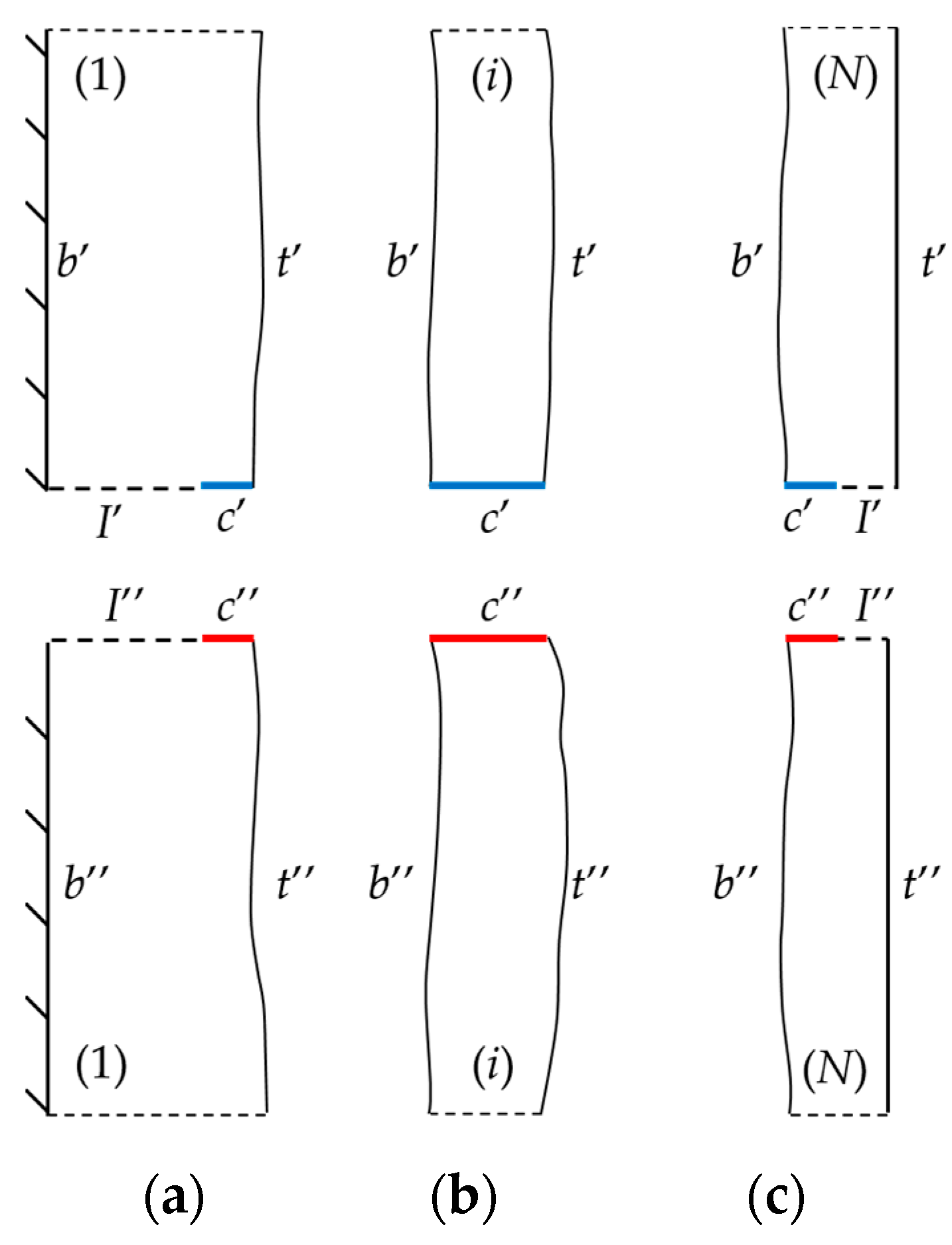
3. Formulation of the Method

We present Figure 2a by rotating Figure 1 by 90 degrees clockwise and by removing the symbols of quantities for visual simplicity. The initial slit-like upper and lower crack surfaces, one of which coincides with the other effectively, are marked in blue and red, respectively, for visual distinguishment. We then divide the media by cutting it along the initial slit-like crack surfaces in order to distinguish the effects of the elements placed along one crack surface from those placed along the other in subsequent numerical implementation, leading to the resultant medium shown in Figure 2b.
We indicate the upper and lower parts of each layer after the cutting by the superscripts ’ and ‘’, respectively (Figure 3). The dividing also results in the horizontal interfaces, denoted by I, in the bottom and top layers, as shown in Figure 3a,c.
(1) For the bottom layer (i = 1):
We define α to represent the boundaries other than the interface I, i.e., the bottom, top, and crack boundaries. After that, we can formulate the boundary element equations based on the direct method for the two parts of the bottom layer:
K1′u1′ = p1′, and K1″u1″ = p1″
where K1′ and K1″ are the coefficient matrices of the upper and lower parts, respectively. They are determined by the configuration of the layer only. Their explicit forms can be found in the work of Crouch and Starfield [34].
We can rewrite Equations (4) to (5) by discretizing with boundary elements and partitioning them according to the categorization of the boundaries:
[ K α α 1 K α I 1 K I α 1 K I I 1 ] { u α 1 u I 1 } = { p α 1 p I 1 } ,   and   [ K α α 1 K α I 1 K I α 1 K I I 1 ] { u α 1 u I 1 } = { p α 1 p I 1 }
Note that the continuity conditions defined by the local coordinates apply to interfaces I’ and I″:
uI = −uI″, pI = pI″
The substitution of Equation (6) into Equation (5) with subsequent algebraic arrangement leads to:
[ H α α 1 H α α 1 H α α 1 H α α 1 ] { u α 1 u α 1 } = { p α 1 p α 1 }
where { H α α 1 = K α α 1 K α I 1 ( K I I 1 + K I I 1 ) 1 K I α 1 H α α 1 = K α I 1 ( K I I 1 + K I I 1 ) 1 K I α 1 H α α 1 = K α I 1 ( K I I 1 + K I I 1 ) 1 K I α 1 H α α 1 = K α α 1 K α I 1 ( K I I 1 + K I I 1 ) 1 K I α 1 ,
and we define a new coefficient matrix H 1 [ H α α 1 H α α 1 H α α 1 H α α 1 ] .
As indicated in the statement of the problem ub1 = 0, the rows and columns pertaining to the bottom boundary can be extracted out of H1, leading to a submatrix H ^ 1 that contains only the quantities on the top and crack boundaries:
[ H t t 1 H t c 1 H c t 1 H c c 1 ] { u t 1 u c 1 } = { p t 1 p c 1 }
In Equation (8), the submatrices with the subscript without prime relate to the boundary elements on the corresponding boundaries of the two parts. For example, Htc1 is the submatrix representing the effects of the elements on the top boundaries of the two parts (both t′ and t″) on the elements on the crack surfaces of the two parts (both c′ and c″).
Equation (8) is in our preferable form, containing only the displacement of the crack surface, which is our target, and the quantities of the top boundary that links to the bottom boundary of upper layers via the continuity condition of Equation (3), enabling a recursive procedure to solve the displacement of the crack surfaces in each layer.
From Equation (8), we have:
uc1 = (Hcc1)−1(pc1Hct1ut1)
The substitution of Equation (9) and the continuity condition Equation (3) into (8) leads to:
p t 1 = [ ( H t t 1 ) 1 H t c 1 ( H c c 1 ) 1 H c t 1 ] u t 1 + H t c 1 ( H c c 1 ) 1 p c 1   = K ^ t t 1 u t 1 + p ^ t 1   = K ^ t t 1 u b 2 + p ^ t 1 = p ^ b 2
The stiffness matrix of the bottom layer K ^ tt1 = (Htt1)−1Htc1(Hcc1)−1Hct1, and p ^ t1 = Htc1 (Hcc1)−1 pc1. Equation (10) links the quantities of the bottom layer to those of the second layer.
(2) For the second layer (I = 2):
As shown in Figure 3b, the cutting results in two separate parts, each of which requires a system of linear algebraic equations:
K2′u2′ = p2′, and K2″u2″ = p2″
or in a more-explicit form:
[ K b b 2 K b c 2 K b t 2 K c b 2 K c c 2 K c t 2 K t b 2 K t c 2 K t t 2 ] { u b 2 u c 2 u t 2 } = { p b 2 p c 2 p t 2 } ,   and   [ K b b 2 K b c 2 K b t 2 K c b 2 K c c 2 K c t 2 K t b 2 K t c 2 K t t 2 ] { u b 2 u c 2 u t 2 } = { p b 2 p c 2 p t 2 }
The explicit forms of the coefficient matrices K2′ and K2″ are also found in the work of Crouch and Starfield [34].
Since the two parts are separate, we can simply “patch” the two equations into one:
[ K 2 0 0 K 2 ] { u 2 u 2 } = { p 2 p 2 }
We define the new coefficient matrix for the second layer H2 [ K 2 0 0 K 2 ] , which is then partitioned according to the categorization of the boundaries along the whole second layer, e.g., both t2′ and t2″ are categorized as t2:
[ H b b 2 H b c 2 H b t 2 H c b 2 H c c 2 H c t 2 H t b 2 H t c 2 H t t 2 ] { u b 2 u c 2 u t 2 } = { p b 2 p c 2 p t 2 }
From the third row, we obtain:
uc2 = (Hcc2)−1(pc2Hct2ut2Hcb2ub2)
The substitution of Equations (15) and (10) into the second row of Equation (14) leads to:
p b 2 = H b t 2 u t 2 + H b b 2 u b 2 + H b c 2 u c 2   = K ^ t t 1 u b 2 + p ^ t 1   = p t 1
Then, we can obtain:
u b 2 = ( A 2 K ^ t t 1 ) 1 B 2 u t 2 +   ( A 2 K ^ t t 1 ) 1 [ H b c 2 ( H c c 2 ) 1 p c 2 p ^ t 1 ]
where A2 = Hbc2(Hcc2)−1 Hcb2Hbb2, and B2 = Hbc2(Hcc2)−1 Hct2Hbt2.
The substitution of Equation (17) into (15) results in:
u c 2 = ( H c c 2 ) 1 [ H c t 2 H c b 2 ( A 2 K ^ t t 1 ) 1 B 2 ] u t 2   + ( H c c 2 ) 1 { [ I H c b 2 ( A 2 K ^ t t 1 ) 1 H b c 2 ( H c c 2 ) 1 ] p c 2 + H c b 2 ( A 2 K ^ t t 1 ) 1 p ^ t 1 }
where I is the identity matrix.
The substitution of Equations (17) and (18) into the first row of (14) leads to the stiffness matrix equation of the second layer:
p t 2 = K ^ t t 2 u t 2 + C 2 p c 2 + D 21 p ^ t 1   = K ^ t t 2 u t 2 + p ^ t 2   = K ^ t t 2 u b 3 + p ^ t 2 = p b 3
where { C 2 = H t c 2 ( H c c 2 ) 1 [ I H c b 2 ( A 2 K ^ t t 1 ) 1 H b c 2 ( H c c 2 ) 1 ] + H t b 2 ( A 2 K ^ t t 1 ) 1 H b c 2 ( H c c 2 ) 1 D 21 = H t c 2 ( H c c 2 ) 1 H c b 2 ( A 2 K ^ t t 1 ) 1 H t b 2 ( A 2 K ^ t t 1 ) 1 p ^ t 2 = C 2 p c 2 + D 21 p ^ t 1 K ^ t t 2 = H t t 2 H t b 2 ( A 2 K ^ t t 1 ) 1 B 2 H t c 2 ( H c c 2 ) 1 [ H c t 2 H c b 2 ( A 2 K ^ t t 1 ) 1 B 2 ]
Having obtained Equation (19), we can treat the remaining inner layers (i runs from 2 to N–1) in the same manner as we did for the second layer. Thus, we can obtain the recursive stiffness equation for the ith layer simply by replacing superscripts 1 and 2 in Equation (19) with i–1 and i, respectively.
p t i = K ^ t t i u t i + p ^ t i
(3) For the top layer (i = N):
The cutting of the top layer results in an interface that is shared by the two resultant upper and lower parts, the same as the bottom layer. Thus, we chose an analogous way that is used from Equations (5) to (10) to treat the top layer, leading to the new coefficient matrix of the top layer:
H N [ H α α N H α α N H α α N H α α N ]
where { H α α N = K α α N K α I N ( K I I N + K I I N ) 1 K I α N H α α N = K α I N ( K I I N + K I I N ) 1 K I α N H α α N = K α I N ( K I I N + K I I N ) 1 K I α N H α α N = K α α N K α I N ( K I I N + K I I N ) 1 K I α N
Unfortunately, the displacements of the bottom boundary of the top layer remain unknown. Thus, we cannot extract the equations associated with them out of the coefficient matrix, as we did for the bottom layer. As a result, we treated the coefficient matrix in the same manner as we did for the second layer to obtain explicit expressions of the displacement of the boundaries of the top layer. The results share the same forms of Equations (17)–(19) by replacing superscripts 1 and 2 with N − 1 and N, respectively, for the top layer:
u b N = ( A N K ^ t t N 1 ) 1 B N u t N +   ( A N K ^ t t N 1 ) 1 [ H b c N ( H c c N ) 1 p c N p ^ t N 1 ]
u c N = ( H c c N ) 1 [ H c t N H c b N ( A N K ^ t t 1 ) 1 B N ] u t N   + ( H c c N ) 1 {   [ I H c b N ( A N K ^ t t N 1 ) 1 H b c N ( H c c N ) 1 ] p c N + H c b N ( A N K ^ t t N 1 ) 1 p ^ t N 1 }
p t N = K ^ t t N u t N + C N p c N + D ( N ) ( N 1 ) p ^ t N 1
where { A N = H b c N ( H c c N ) 1 H c b N H b b N B N = H b c N ( H c c N ) 1 H c t N H b t N C N = H t c N ( H c c N ) 1 [ I H c b N ( A N K ^ t t N 1 ) 1 H b c N ( H c c N ) 1 ] + H t b N ( A N K ^ t t N 1 ) 1 H b c N ( H c c N ) 1 D ( N ) ( N 1 ) = H t c N ( H c c N ) 1 H c b N ( A N K ^ t t N 1 ) 1 H t b N ( A N K ^ t t N 1 ) 1 p ^ t N = C N p c N + D ( N ) ( N 1 ) p ^ t N 1 K ^ t t N = H t t N H t b N ( A N K ^ t t N 1 ) 1 B N H t c N ( H c c N ) 1 [ H c t N H c b N ( A N K ^ t t N 1 ) 1 B N ]
It is obvious from the stiffness matrix equation, Equation (24), that we can obtain utN easily when ptN is prescribed as a boundary condition of the whole multilayered media since all of the other quantities on the right-hand side of Equation (24) are known:
u t N = ( K ^ t t N ) 1 p t N C N p c N D ( N ) ( N 1 ) p ^ t N 1
The substitution of the calculated utN into Equations (22) and (23) solves ubN and ucN, respectively, since all of the other quantities on the right-hand sides of the two equations are known. Then, we can obtain ut N−1 via the interface continuity condition utN−1 = −ubN. After that, we can obtain ub N−1 and uc N−1 in the same manner as we calculated ubN and ucN, enabling a sequential computation that solves the displacements on the top boundary, crack surface, and bottom boundary of each layer in descending order from the very top layer to the very bottom one. It is worth noting that if utN is given as a boundary condition of the whole system, then we can start the sequential computation directly without Equation (25). Therefore, our method is applicable for any prescribed boundary condition at the very top surface and are not limited to the traction-given boundary condition.
Because we are particularly interested in the displacement of the crack surface uci, it is more efficient that the displacement ubi and uti both be expressed in terms of uci so that only uci is involved in the computation. Equations (17) and (18) give the expressions of ubi and uci by replacing superscripts 1 and 2 with i–1 and i, respectively, for the inner layer:
u b i =   ( A i K ^ t t i 1 ) 1 B i u t i + ( A i K ^ t t i 1 ) 1 [ H b c i ( H c c i ) 1 p c i p ^ t i 1 ]
u c i = ( H c c i ) 1 [ H c t i H c b i ( A i K ^ t t i 1 ) 1 B i ] u t i   + ( H c c i ) 1 { [ I H c b i ( A i K ^ t t i 1 ) 1 H b c i ( H c c i ) 1 ] p c i + H c b i ( A i K ^ t t i 1 ) 1 p ^ t i 1 }
From Equation (27), we have:
u t i = H ^ t t i H t c i H c c i u c i H ^ t t i H t c i p ˜ c i
The substitution of Equation (27) into (25) leads to:
u b i = H ^ b c i u c i + u ^ b i
where { H ^ t t i = { H t c i [ H c t i H c b i ( A i K ^ t t i 1 ) 1 B i ] } 1 p ˜ c i = [ I H c b i ( A i K ^ t t i 1 ) 1 H b c i ( H c c i ) 1 ] p c i + H c b i ( A i K ^ t t i 1 ) 1 p ^ t i 1 H ^ b c i = ( A i K ^ t t i 1 ) 1 B i H ^ t t i H t c i H c c i u ^ b i = ( A i K ^ t t i 1 ) 1 [ B i H ^ t t i H t c i p ˜ c i + H b c i ( H c c i ) 1 p c i p ^ t i 1 ]
The combination of Equation (28) and the interface continuity condition −uti−1 = ubi gives:
u c i 1 = H c t i H ^ t t i 1 H t c i 1 H c c i 1 1 H c t i 1 H ^ b c i u c i + u ^ b i + H ^ t t i 1 H t c i 1 p ˜ c i 1
Equation (30) is valid for the inner layers; thus, i ranges from 3 to N for Equation (30).
For the bottom layer, the combination of Equation (29) with i = 2 and Equation (9) leads to:
u c 1 = ( H c c 1 ) 1 [ p c 1 + H c t 1 u t 1 ( H ^ b c 2 u c 2 + u ^ b i ) ]
Once utN is determined from Equation (25) or given directly as a prescribed boundary condition, we can solve ucN with Equation (23), enabling a sequential computation to solve the displacements on the crack surfaces consecutively in each layer in a descending order from the very top layer to the very bottom one with Equations (30) and (31). The solved crack surface displacement in all of the layers uc contains two parts: the displacement on the upper crack surfaces, denoted by uc+, and that on the lower crack surfaces, denoted by uc. According to the local coordinate defined in [34], the crack opening displacement Dc is (see Appendix A for details):
Dc = uc + uc+

4. Results and Discussion
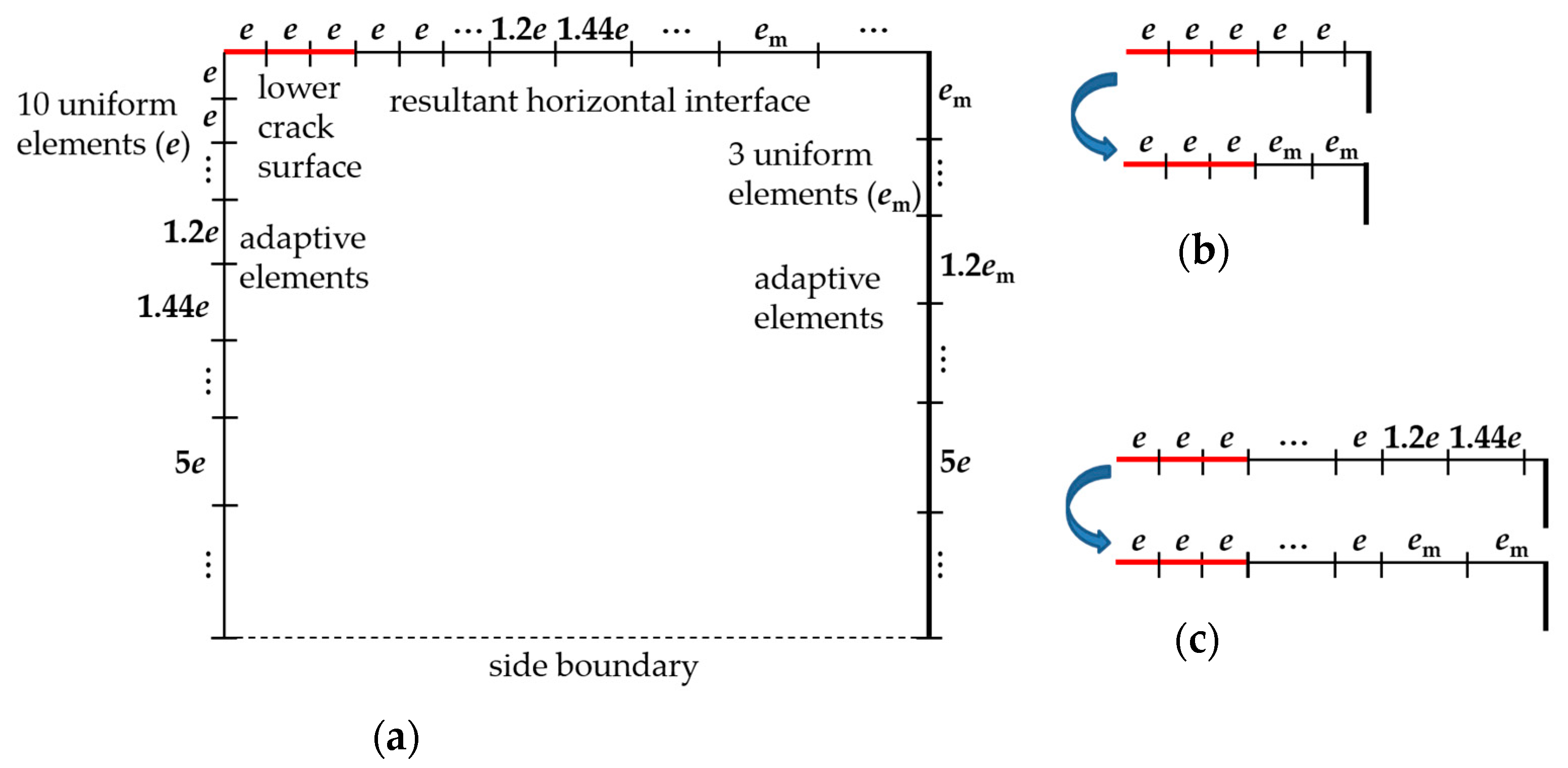
We shall demonstrate the results of three numerical examples to validate the accuracy and efficiency of the consecutive stiffness method (CSM) that is proposed in the previous section. A slit-like crack subjected to known normal traction perpendicularly intersects the interfaces, if any, which are assumed to be parallel, so that other methods can be used as benchmarks. The contrasts in Young’s modulus and the thickness of the layer maintain an order of magnitude, which falls within the range of practical fracturing treatment [15,38,39].
We defined the percentage error of a method as follows:
Err % = D 1 D 0 D 0 × 100 %
where D1 is the crack opening obtained by the method to be tested, and D0 represents the crack opening determined by the benchmark method.

4.1. Discretization

Figure 4 illustrates the discretization of the lower part of the top layer in our numerical examples schematically. We divided the whole initial slit-like crack surface into elements of a uniform size e, which was chosen carefully so that there would be sufficient space for at least two elements that are uniform in size e on the resultant horizontal interface (Figure 4b). After that, we placed adaptive elements on the bottom boundary (interfaces of the multilayered elastic media) of the top layer. We made sure that ten uniform elements in the same size e were placed adjacent to the crack surface. Then, we placed a series of elements, of which an element is 1.2 times larger than its previous one in size. When the size of an element became more than 5e, we made the elements and all of the following ones 5e in size exactly, preventing computational issues due to sharp contrasts in element size. As a result, we acquired an interface of one part in a size that is only slightly larger than 50l, in which l is half the length of the initial crack surface, as shown in Figure 5a.
We placed adaptive elements on the horizontal interface in the similar way. If the interface is too short for 10 uniform elements in size e, we removed the last two elements and introduced two new uniform elements in size em by dividing the remaining part in two evenly (Figure 4b). When the interface was longer than 10 uniform elements in size e, we used the same approach to treat the elements at the corner of the horizontal interface and the top surface (Figure 4c), preventing sharp contrasts in element size. After finishing the discretization of the horizontal interface, we chose a similar approach to discretize the top surface of the multilayered system. We first placed three elements that were uniform in size em with subsequent adaptive elements of which the maximum size does not exceed 5e. When the discretization became close to the corner of the top surface and the side boundary, we used the treatment shown in Figure 4b,c to determine the size of the last two elements on the top surface. Having completed the discretization of the lower part, we discretized the upper part using symmetry with respect to the crack surface. As a result, the distance of the two side boundaries h becomes about 100l, as shown in Figure 5a, approximating the condition of remote side boundaries (h→∞).
The approach to discretize the top layer also applies to the bottom layer. As for the inner layers, if any, discretization becomes simpler since there is no horizontal interface due to the division. We can discretize the two vertical interfaces in the same manner that we discretized the bottom boundary of the top layer, as illustrated in Figure 5b.

4.2. Homogeneous Medium

The first example is the calculation of the opening displacement of a crack under a known constant normal loading p1 in an infinite homogeneous and isotropic plane (Figure 6).
The analytical solution to crack opening in the homogeneous medium is [31]:
D 0 = 4 ( 1 v 2 ) E p 1 l 2 x 2
Then, the percentage errors of the DDM and the DM with respect to the analytical solution with different numbers of crack elements are illustrated in Figure 7, in which only the left-half part of the crack has been presented due to symmetry. The abscissa is normalized by x/l so that the coordinate −1 represents the crack tip. Figure 7b involves 100 crack elements, while only 11 elements are shown for visual simplicity.
Figure 7 clearly demonstrates that more-refined discretization leads to better accuracy along the whole crack surface, except at the crack tip, where the DDM yields an error that is almost twice that of the DM. The DM shows more satisfying accuracy than the DDM, particularly at the tip, since the integrals involved in the implementation of the DM can be evaluated analytically under the plane-strain condition and because the singularity at the tip of the DDM is stronger than that of the DM [28,29,34].

4.3. Two Bonded Half Planes

The second numerical example is the computation of the opening displacement of a crack that passes through two bonded half planes under known normal loading (Figure 8), in which the abscissa is normalized by
ξ = 2 x b 1 b 1 , x < 0 2 x b 2 b 2 , x 0
We assume that the loading satisfies an additional continuity condition (Equation (36)) so that a semi-analytical solution can be used as a benchmark [40], although neither the DDM nor the DM requires such an extra condition for implementation.
1 v 1 2 E 1 p 1 = 1 v 2 2 E 2 p 2
In addition, the two half planes are characterized by E1, v1 and E2, v2, respectively. We set E1 = 3.07(GPa), v1 = 0.35; E2 = 68.95(Gpa), and v2 = 0.3 and present the percentage errors of the DDM and the consecutive stiffness method (CSM) with respect to the semi-analytical solution in Figure 9 with different b1/b2 values. The thickness of layer d is set to be equal to 100 times that of the larger one of b1 and b2, approximating the condition of infinite d. We placed 10 uniform elements on the shorter segment of the crack surface.
Figure 9 illustrates that both methods match the benchmark along the crack surface well, except at the tip, where the CSM yields errors that are lower than 20%, which is acceptable for practical engineering applications. Furthermore, the CSM leads to generally satisfactory results when the ratio of crack segments falls in a practical range. The first and second numerical examples demonstrated the more-satisfactory accuracy of our CSM compared to the DDM.

4.4. General Multilayered Media

The third numerical example computes the opening displacement of a crack intersecting a few layers under constant loading p0 in a general multilayered media in which the number of layers is equal to or larger than three. The DDM fails in such a case since there is no analytical fundamental solution for it. Thus, we compared the efficiency of the CSM and that of the conventional DM, which led to a large system of equations and solved all of the unknowns simultaneously. We set the crack being distributed uniformly in the system so that the length of each crack segment was l1, as shown in Figure 10. Ten elements were placed on each crack segment. The thicknesses of the bottom and top layers were both set to 100l1, approximating the condition of their infinite thicknesses. We set E1 = 5(GPa), v1 = 0.3; E2 = 50(Gpa), and v2 = 0.25.
The durations required by the CSM and the conventional DM to solve the crack opening displacement are listed in Table 1. The computation was conducted with MATLAB 2014a on a laptop with an Intel(R) Core(TM) i7-2720QM CPU and 12GB RAM. The table clearly indicates that our CSM is more efficient than the conventional DM. The contrast becomes even larger with an increase in the number of layers, which leads to more elements being involved in the computation.
The three numerical examples clearly demonstrate the better accuracy and broader applicability of our method compared to the DDM, and more-acceptable efficiency of our method compared to the conventional DM.

5. Conclusions

We have proposed a numerical method based on the DM for crack problems in a multilayered elastic media consisting of a set of individually homogeneous strata. The method distinguishes the effects of elements placed along one crack surface from those placed along another crack surface by dividing the whole media along the initial slit-like crack surface. After that, we derived a recursive formula that obtains a “stiffness matrix” for each layer by exploiting the chain-like feature of the system, enabling a sequential computation to solve the displacements on the crack surface in each layer “consecutively” in a descending order from the very top layer to the very bottom one. In addition, the final system of equations in our method only contains the unknown displacements on the crack surfaces, ensuring the efficiency of the method. The numerical examples demonstrate the better accuracy and broader applicability of our method compared to the DDM and more-acceptable efficiency compared to the conventional DM, making it a convincing benchmark to test new methods for crack problems in multilayered elastic media. We are planning to conduct analysis of crack problems using our method in complex geometry, which fails the FT-based methods, and under complicated loading, which fails the DDM.

Author Contributions

Conceptualization, G.L. and G.X.; methodology, G.L. and B.X.; validation, Y.L. and W.X.; formal analysis, P.Z. and J.Z.; writing—original draft preparation, G.L.; editing, G.X. and B.X.; supervision, G.X. and B.X.; project administration, G.X. and B.X.; funding acquisition, G.L. and B.X. All authors have read and agreed to the published version of the manuscript.

Funding

This work was supported by the National Natural Science Foundation of China (No. 52004183).

Data Availability Statement

Not applicable.

Acknowledgments

The authors appreciate Petro-China Research Institute of Petroleum Exploration & Development, FrackOptima Inc.; Shell International Exploration and Production Inc.; and ConocoPhillips for the technical support.

Conflicts of Interest

The authors declare no conflict of interest.

Appendix A

The local coordinate adopted in our study follows the convention that the normal direction points outwards from the surface of the domain of interest and that the shear direction obeys the right-hand rule with respect to the normal one (Figure A1a).
Figure A1a shows the displacement and traction on a pair of interface elements (1) and (2). We set |u1| = |u2| = u0 and|p1| = |p2| = p0, where u0 and p0 are the magnitudes of the displacement and traction, respectively. According to the interface continuity, we have u1 = u2 = u0 and p1 = −p2 = p0 under the global coordinates (x, y). The local coordinates of Element (1) and (2), denoted by (x1, y1) and (x2, y2), respectively, however, are constructed as illustrated in Figure A1a based on the convention explained above. As a result, u1 = −u0 and p1 = p0 for Element (1), and u2 = u0 and p2 = p0 for Element (2). Therefore, the interface continuity under the local coordinates is:
u1 = −u2, p1 = p2
Figure A1. The local coordinates for (a) interface elements and for (b) the calculation of opening displacement [34].
Mathematics 10 04403 g0a1
Figure A1b illustrates the displacements of a pair of crack surface elements, denoted by u+ and u for the upper elements and lower elements, respectively, due to the loading conditions p. The local coordinates of the two elements are constructed based on the convention. Thus, u+ = −|u+|, and u = −|u|. The opening displacement D is defined as the relative displacement of the lower element with respect to the upper one [34]. Thus:
D = −|u| − |u+| = u + u+
Equations (A1) and (A2) correspond to Equations (3) and (32), respectively.
The Appendix A only presents the essence of the local coordinates, the details of which can be found in the work of Crouch and Starfield [34].

References

  1. Toroody, F.; Khalaj, S.; Leoni, L.; Carlo, F.; Bona, G.; Forcina, A. Reliability Estimation of Reinforced Slopes to Prioritize Maintenance Actions. Int. J. Environ. Res. Public Health 2021, 18, 373. [Google Scholar]
  2. Xiao, B.; Fang, J.; Long, G.; Tao, Y.; Huang, Z. Analysis of thermal conductivity of damaged tree-like bifurcation network withfractal roughened surfaces. Fractals 2022, 30, 2250104. [Google Scholar] [CrossRef]
  3. An, S.; Zou, H.; Li, W.; Deng, Z. Experimental investigation on the vibration attenuation of tensegrity prisms integrated with particle dampers. Acta Mech. Solida Sin. 2022, 35, 672–681. [Google Scholar] [CrossRef]
  4. Hamzah, K.; Long, N.; Senu, N.; Eshkuvatov, K. Numerical solution for crack phenomenon in dissimilar materials under various mechanical loadings. Symmetry 2021, 13, 235. [Google Scholar] [CrossRef]
  5. Xiao, B.; Wang, W.; Zhang, X.; Long, G.; Fan, J.; Chen, H.; Deng, L. A novel fractal solution for permeability and Kozeny-Carman constant of fibrous porous media made up of solid particles and porous fibers. Powder Technol. 2019, 349, 92–98. [Google Scholar] [CrossRef]
  6. Liang, M.; Liu, Y.; Xiao, B.; Yang, S.; Wang, Z. An analytical model for the transverse permeability of gas diffusion layer with electrical double layer effects in proton exchange membrane fuel cells. Int. J. Hydrog. Energ 2018, 43, 17880–17888. [Google Scholar] [CrossRef]
  7. Xiao, B.; Li, Y.; Long, G. A fractal model of power-law fluid through charged fibrous porous media by using the fractional-derivative theory. Fractals 2022, 30, 2250072. [Google Scholar] [CrossRef]
  8. Cantini, A.; Leoni, L.; Carlo, F.; Salvio, M.; Martini, C.; Martini, F. Technological Energy Efficiency Improvements in Cement Industries. Sustainability 2021, 13, 3810. [Google Scholar] [CrossRef]
  9. Liang, M.; Fu, C.; Xiao, B.; Luo, L.; Wang, Z. A fractal study for the effective electrolyte diffusion through charged porous media. Int. J. Heat Mass Transf. 2019, 137, 365–371. [Google Scholar] [CrossRef]
  10. Cheng, W.; Lu, C.; Feng, G.; Xiao, B. Ball sealer tracking and seating of temporary plugging fracturing technology in the perforated casing of a horizontal well. Energy Explor. Exploit. 2021, 39, 2045–2061. [Google Scholar] [CrossRef]
  11. Adachi, J.; Siebrits, E.; Peirce, A.; Desroches, J. Computer simulation of hydraulic fractures. Int. J. Rock Mech. Min. Sci. 2007, 44, 739–757. [Google Scholar] [CrossRef]
  12. Long, G.; Liu, S.; Xu, G.; Wong, S.; Chen, H.; Xiao, B. A perforation-erosion model for hydraulic-fracturing applications. SPE Prod. Oper. 2018, 33, 770–783. [Google Scholar] [CrossRef]
  13. Cheng, W.; Lu, C.; Xiao, B. Perforation optimization of intensive-stage fracturing in a horizontal well using a coupled 3D-DDM fracture model. Energies 2021, 14, 2393. [Google Scholar] [CrossRef]
  14. Cui, C.; Zhang, Q.; Banerjee, U.; Babuška, I. Stable generalized finite element method (SGFEM) for three-dimensional crack problems. Numer. Math. 2022, 152, 475–509. [Google Scholar] [CrossRef]
  15. Liu, S.; Valko, P. A rigorous hydraulic-fracture equilibrium-height model for multilayer formations. SPE Prod. Oper. 2018, 33, 214–234. [Google Scholar] [CrossRef]
  16. Peirce, A.; Siebrits, E. The scaled flexibility matrix method for the efficient solution of boundary value problems in 2D and 3D layered elastic media. Comput. Methods Appl. Mech. Eng. 2001, 190, 5935–5956. [Google Scholar] [CrossRef]
  17. Liu, S.; Valko, P.; McKetta, S.; Liu, X. Microseismic closure window characterizes hydraulic-fracture geometry better. SPE Reserv. Eval. Eng. 2017, 20, 423–445. [Google Scholar] [CrossRef]
  18. Long, G.; Xu, G. The effects of perforation erosion on practical hydraulic-fracturing applications. SPE J. 2017, 22, 645–659. [Google Scholar] [CrossRef]
  19. Cheng, W.; Jin, Y.; Chen, M.; Jiang, G. Numerical stress analysis for the multi-casing structure inside a wellbore in the formation using the boundary element method. Pet. Sci. 2017, 14, 126–137. [Google Scholar] [CrossRef] [Green Version]
  20. Long, G.; Xu, G. A combined boundary integral method for analysis of crack problems in multilayered elastic media. Int. J. Appl. Mech. 2016, 8, 1650070. [Google Scholar] [CrossRef]
  21. Cheng, W.; Jiang, G.; Xie, J.; Wei, Z.; Zhou, Z.; Li, X. A simulation study comparing the Texas two-step and the multistage consecutive fracturing method. Pet. Sci. 2019, 16, 1121–1133. [Google Scholar] [CrossRef]
  22. Blandford, G.; Ingraffea, A.; Liggett, J. Two-dimensional stress intensity factor computations using the boundary element method. Int. J. Numer. Methods Eng. 1981, 17, 387–404. [Google Scholar] [CrossRef]
  23. Peirce, A.; Siebrits, E. Uniform asymptotic approximations for accurate modeling of cracks in layered elastic media. Int. J. Fract. 2001, 110, 205–239. [Google Scholar] [CrossRef]
  24. Thompson, W. Transmission of elastic waves through a stratified medium. J. Appl. Phys. 1950, 21, 89–93. [Google Scholar] [CrossRef]
  25. Gilbert, F.; Backus, G. Propagator matrices in elastic wave and vibration problems. Geophysics 1966, 31, 326–332. [Google Scholar] [CrossRef]
  26. Buffler, H. Theory of elasticity of a multilayered medium. J. Elast. 1971, 1, 125–143. [Google Scholar] [CrossRef]
  27. Benitez, F.; Rosakis, A. Three-dimensional elastostatics of a layer and a layered medium. J. Elast. 1987, 18, 3–50. [Google Scholar] [CrossRef]
  28. Shou, K.; Napier, J. A two-dimensional linear variation displacement discontinuity method for three-layered elastic media. Int. J. Rock Mech. Min. Sci. 1999, 36, 719–729. [Google Scholar] [CrossRef]
  29. Shou, K. A superposition scheme to obtain fundamental boundary element solutions in multi-layered elastic media. Int. J. Numer. Anal. Methods Geomech. 2000, 24, 795–814. [Google Scholar] [CrossRef]
  30. Crouch, S. Solution of plane elasticity problems by the displacement discontinuity method. Int. J. Numer. Methods Eng. 1976, 10, 301–343. [Google Scholar] [CrossRef]
  31. Asaro, R.; Lubarda, V. Mechanics of Solids and Materials; Cambridge University Press: New York, NY, USA, 2006. [Google Scholar]
  32. Siebrits, E.; Crouch, S. On the paper ‘A two-dimensional linear variation displacement discontinuity method for three-layered elastic media’ by Keh-Jian Shou and J.A.L. Napier, International Journal of Rock Mechanics and Mining Sciences, Vol. 36(6), 719–729, 1999. Int. J. Rock Mech. Min. Sci. 2000, 37, 873–875. [Google Scholar] [CrossRef]
  33. Shou, K.; Napier, J. Author’s reply to discussion by E. Siebrits and S. L. Crouch regarding the paper ‘A two-dimensional linear variation displacement discontinuity method for three-layered elastic media’, Keh-Jian Shou and J.A.L. Napier, International Journal of Rock Mechanics and Mining Sciences, Vol. 36, 719–729, 1999. Int. J. Rock Mech. Min. Sci. 2000, 37, 877–878. [Google Scholar]
  34. Crouch, S.; Starfield, A. Boundary Element Methods in Solid Mechanics; George Allen & Unwein: London, UK, 1983. [Google Scholar]
  35. Zheng, R.; Deng, Z. External circular crack problem in magneto–electro-elasticity: Shear mode. Eng. Fract. Mech. 2022, 266, 108374. [Google Scholar] [CrossRef]
  36. Maier, G.; Novati, G. On boundary element-transfer matrix analysis of layered elastic systems. Eng. Anal. 1986, 3, 208–216. [Google Scholar] [CrossRef]
  37. Maier, G.; Novati, G. Boundary element elastic analysis of layered soils by a successive stiffness method. Int. J. Numer. Anal. Methods Geomech. 1987, 11, 435–447. [Google Scholar] [CrossRef]
  38. Xiao, B.; Huang, Q.; Chen, H.; Chen, X.; Long, G. A fractal model for capillary flow through a single tortuous capillary with roughened surfaces in fibrous porous media. Fractals 2021, 29, 2150017. [Google Scholar] [CrossRef]
  39. Zhang, Q.; Cui, C.; Banerjee, U.; Babuška, I. A condensed generalized finite element method (CGFEM) for interface problems. Comput. Methods Appl. Mech. Eng. 2022, 391, 114537. [Google Scholar] [CrossRef]
  40. Erdogan, F.; Biricikoglu, V. Two bonded half planes with a crack going through the interface. Int. J. Eng. Sci. 1973, 11, 745–766. [Google Scholar] [CrossRef]
Figure 1. Schematic view of the crack problem [37].
Mathematics 10 04403 g001
Figure 2. (a) Division of the media containing a slit-like crack; (b) results of the division.
Mathematics 10 04403 g002
Figure 3. Different boundaries of (a) the bottom layer; (b) inner layer; and (c) the top layer.
Mathematics 10 04403 g003
Figure 4. Schematic view of (a) discretization of the lower part of the top layer; (b) treatment of the elements adjacent to the corner when the horizontal interface is short; and (c) treatment of the elements adjacent to the corner when the horizontal interface is long.
Mathematics 10 04403 g004
Figure 5. Schematic view of (a) crack surface, interfaces, and side boundaries; (b) discretization of the lower part of an inner layer.
Mathematics 10 04403 g005
Figure 6. Schematic view of the crack problem in homogeneous medium.
Mathematics 10 04403 g006
Figure 7. Percentage errors of the DDM and the DM with (a) 5 crack elements and (b) 100 crack elements.
Mathematics 10 04403 g007
Figure 8. Schematic view of the crack problem in two bonded half planes.
Mathematics 10 04403 g008
Figure 9. Percentage errors of the DDM and the CSM with b1/b2 = (a) 1/25; (b) 1/1; and (c) 2/1.
Mathematics 10 04403 g009
Figure 10. Schematic view of a crack intersecting a multilayered media containing (a) 3 layers and (b) 5 layers.
Mathematics 10 04403 g010
Table 1. Durations of the CSM and the conventional DM.
MethodDuration for 3 Layers (s)Duration for 5 Layers (s)
CSM58101
DM194406
Publisher’s Note: MDPI stays neutral with regard to jurisdictional claims in published maps and institutional affiliations.

