
Detection and Prediction of Chipping in Wafer Grinding Based on Dicing Signal

1
Department of Computer Science and Information Engineering, National University of Kaohsiung, Kaohsiung 81148, Taiwan
2
Department of Fragrance and Cosmetic Science, Kaohsiung Medical University, Kaohsiung 80708, Taiwan
*
Author to whom correspondence should be addressed.
Mathematics 2022, 10(24), 4631; https://0-doi-org.brum.beds.ac.uk/10.3390/math10244631
Submission received: 21 October 2022
/
Revised: 4 December 2022
/
Accepted: 5 December 2022
/
Published: 7 December 2022
(This article belongs to the Special Issue From Edge Devices to Cloud Computing and Datacenters: Emerging Machine Learning Applications, Algorithms, and Optimizations)
Abstract
:Simple regression cannot wholly analyze large-scale wafer backside wall chipping because the wafer grinding process encounters many problems, such as collected data missing, data showing a non-linear distribution, and correlated hidden parameters lost. The objective of this study is to propose a novel approach to solving this problem. First, this study uses time series, random forest, importance analysis, and correlation analysis to analyze the signals of wafer grinding to screen out key grinding parameters. Then, we use PCA and Barnes-Hut t-SNE to reduce the dimensionality of the key grinding parameters and compare their corresponding heat maps to find out which dimensionality reduction method is more sensitive to the chipping phenomenon. Finally, this study imported the more sensitive dimensionality reduction data into the Data Driven-Bidirectional LSTM (DD-BLSTM) model for training and predicting the wafer chipping. It can adjust the key grinding parameters in time to reduce the occurrence of large-scale wafer chipping and can effectively improve the degree of deterioration of the grinding blade. As a result, the blades can initially grind three pieces of the wafers without replacement and successfully expand to more than eight pieces of the wafer. The accuracy of wafer chipping prediction using DD-BLSTM with Barnes-Hut t-SNE dimensionality reduction can achieve 93.14%.
Keywords:
wafer grinding; backside wall chipping; importance analysis; random forest; dimensionality reduction; Data Driven-Bidirectional LSTMMSC:
68T071. Introduction
In the promotion of Industry 4.0, innovative technology has brought significant reforms to factories, introducing technologies such as cloud computing, big data, the internet of things, and process simulation into factories, significantly increasing factory production capacity. Although the traditional statistical process control (SPC) has been applied widely in factories, Texas Instruments (TI) has proposed new generation approaches using advanced process control (APC) [1,2] or advanced equipment control (AEC) in cooperation with the US military in 1993. TI has tested and improved these process controls over the past ten years. In recent years, many fabs have introduced high-end process technology running in a small amount or across the board with the procedure initially from proof of concept (POC), then proof of service (POS), and finally proof of business (POB). In fierce market competition, fabs focus on APC to improve process control, AEC to enhance equipment efficiency, and other methods to reduce wafer manufacturing costs.
In the wafer grinding process, the fab has to analyze the machine-generated data to understand whether or not there are some signs or common points available before wafer backside wall chipping (or called the wafer chipping) has occurred. If so, people can implement preventive measures to avoid this situation as much as possible. Technically speaking, correlation analyses such as Spearman [3,4,5], Pearson [6,7], and Kendall [8] can analyze the correlation between the wafer grinding parameters. People can determine whether the data is linear and continuous and which method is appropriate for data correlation analysis. In consideration of this, it is not a matter of only looking at a single grinding parameter in the changes; instead, correlations among all of the key grinding parameters must be examined and the changes in all of them with different combinations when wafer chipping has occurred must be observed.
Advanced semiconductor manufacturing processes are all controlled by sophisticated and complex production machines, and the fab can control the process precisely, making the control parameters of these production machines hundreds or thousands. As long as there is a slight deviation of any key parameter, it may cause a deviation in the process, reducing the wafer production yield or scraping it. The fabs will cause unpredictable emergencies due to early equipment function problems in the wafer grinding process. For example, when the production line is grinding wafers, it may be affected by different factors, such as the wear of the blades, the temperature of the cooling water, and even the emission of the cleaning gas. These situations will have a significant impact on throughput and yield.
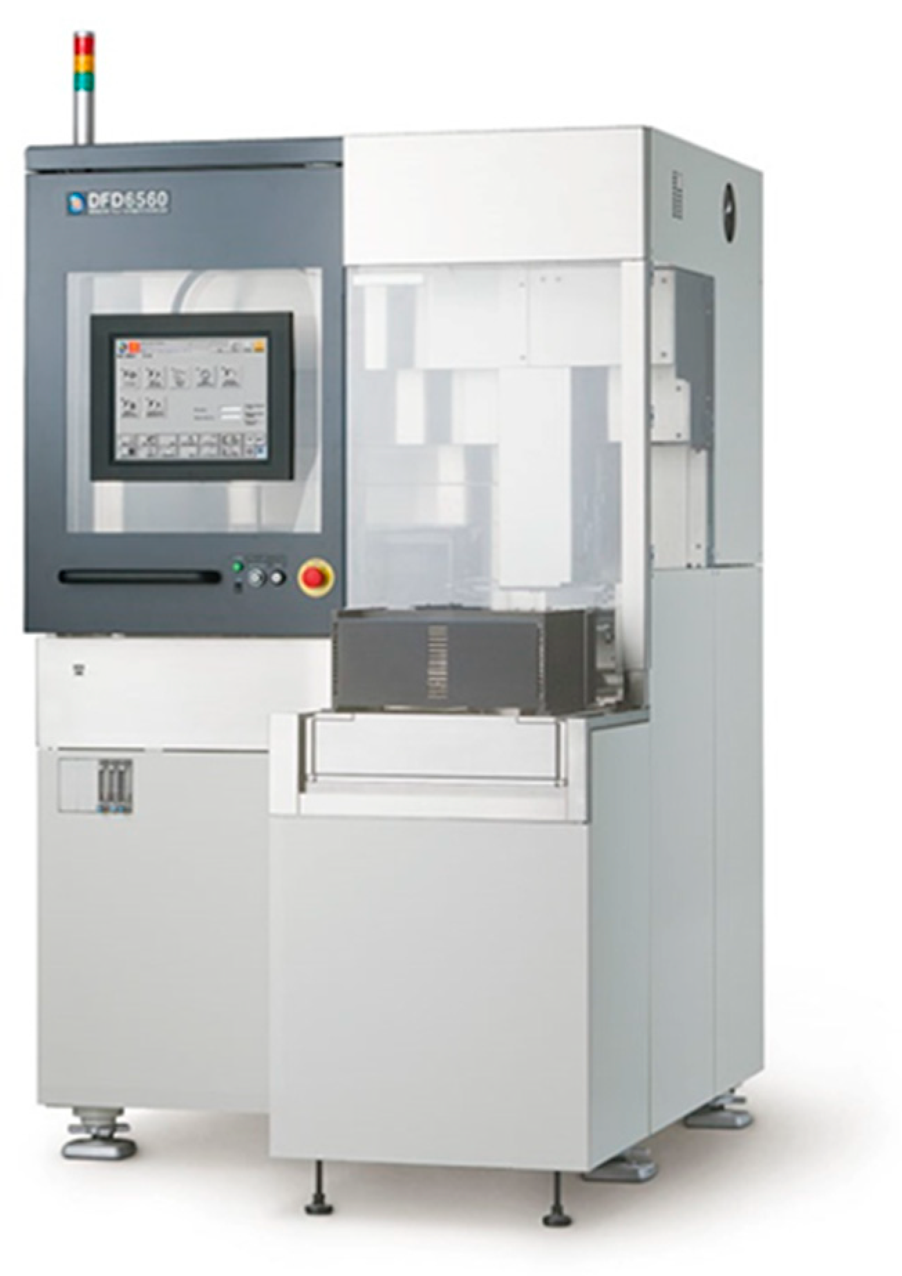
There are still many wafer grinding processes in fabs using early grinding machines (e.g., DFD6560). The production machine often judges the changes in the grinding signals for adjusting the key grinding parameters in the grinding process to reduce the occurrence of large-scale wafer chipping. Technically, simple regression cannot wholly analyze large-scale wafer backside wall chipping because the wafer grinding process encounters many problems. First, wafer grinding machines often miss some of the collected chipping data. In other words, the collected data is incomplete. Second, the collected chipping data presents a non-linear distribution. Third, simple regression may not mine hidden parameters with correlations from the collected data. Therefore, this study has proposed an approach to detect and predict chipping happening in the wafer grinding process, which can adequately adjust the key grinding parameters in time to reduce the occurrence of large-scale chipping, which can increase the wafer grinding yield, and also reduce the loss of the manufacture costs significantly.
2. Related Work
2.1. Literature Review
Based on fault detection and classification, abbreviated FDC [9,10], the production machine will upload the manufacturing parameters to the server or database in the semiconductor manufacturing process, as shown in Figure 1. After receiving the manufacturing parameters, the server and database will use data analysis or related algorithms. The data analysis will issue abnormal indicators when an abnormal situation has occurred. With the ability to monitor, improve, and predict these abnormal indicators, the production machine can detect and classify abnormal situations as early as possible and make the corrections timely, increasing the production yield and reducing the loss of manufacturing costs.
The fab uses sophisticated and complex machines to control the wafer grinding process. With the improved technology of the wafer grinding process, the fab can quickly monitor abnormal machine operations and rapidly respond to the appropriate treatment. FDC is one of the essential techniques for watching the wafer grinding process. From the initially set range of grinding parameters, FDC can instantly detect the deviation of the grinding parameters and issue a warning when the grinding parameters deviate. People can develop a set of early warning functions combined with FDC to foresee or predict the abnormal situations that may inevitably arise in the production machine. According to the abnormal situation predicted in the wafer grinding, we can take preventive measures to avoid wafer chipping, improving the wafer grinding yield and production capacity significantly.
In recent years, big data analytics have been dealing with enormous amounts of data for analysis and processing [11]. In addition, people can apply correlation analysis [12] to understand the correlation between variables and data analysis with a time series [13] to observe the trend of the data stream. Moreover, the technique of machine learning is becoming more and more critical for intelligent data-driven applications. Notably, the importance analysis can screen out random variables that highly impact a stochastic process. Random forest [14,15] can estimate which key parameters are essential in deciding a judgment. Random forests are relatively simple in the estimation method compared with deep learning approaches. Therefore, random forests are much easier and faster than deep learning approaches to find critical factors in a stochastic process.
In the literature review of wafer manufacture-related topics and process-related studies, it is necessary to retest the grinding wafer through the wafer surface depression before wafer assembly. This retest can avoid the situation that induces multiple wafers damaged simultaneously after assembling the defective wafers. Thus, we can reduce the loss of wafer manufacturing costs. The manufacturing process of various fabs frequently adopts this way. The paper [16] has mentioned that many state-of-the-art models for detecting wafer surface chipping phenomena are available for training models in practice. In addition, the article [17] has described a large amount of data in online databases to enable users to train and validate their models with data provided by others.
Furthermore, we are looking for a way to reduce the loss of production costs by using FDC to prevent the chipping from the wafer grinding process as much as possible in advance. Although most of the current literature [18] only uses simple statistics or machine learning to analyze the machine-generated data from time to time, the prediction of the chipping situation in the wafer grinding process is still not very good. Nevertheless, the study [19] has proposed long short-term memory (LSTM) and Bidirectional LSTM (BLSTM) models to show extremely high accuracy for data prediction with a time series. Meanwhile, it has also shown the comparison of the prediction accuracy between the two models. In short, the BLSTM model yielded a better result in the experiments. Moreover, the work [20] has launched many BLSTM models to predict abnormal signals and achieve good jobs. Therefore, this study adopts the BLSTM model to predict large-scale wafer-chipping situations.
In addition to the BLSTM model, the paper [21] has evaluated the performance of various models for time series applications. Based on MSDR, they developed a GMSDR that can perform well in the data set they used in the paper. However, this proposal is unsuitable for the experiments of our study because of a large amount of missing data on the machines and the nonlinear distribution of the collected data. The work [22] also proposed an approach whose framework can implement multiple DGCNs in the application process. DGCN has a solid ability to find essential parameters and use them to improve the accuracy of model predictions. However, it lacks the generalization to infer diversification because it is easier to overfit. The method [23] has proposed a way to help find correlations among various hidden parameters. The proposed deep learning framework can find the correlated hidden parameters in the data collected in their study better than a simple correlation analysis. However, the experimental data in our study comes from the wafer grinding machines, and they lack integrity when compared with the data set used in the method. In other words, our study cannot apply this method because it would possibly lead to overfitting to excessively find out the hidden relationship between various unimportant grinding parameters.
AI applications frequently require simplifying the data complexity to ease the computation burden and improve execution performance. Therefore, dimensionality reduction reduces the size of a vector from a high-dimensional vector to a low-dimensional vector for lowering the computation burden in many AI applications, such as clustering and classification. The paper [24] analyzed the traditional linear dimensionality reduction method PCA and proposed a new-PCA method. The new-PCA method performs feature screening through thresholding and uses entropy to optimize the dimensionality reduction effect. Compared with traditional PCA, it can run faster and obtain more dimensionality reduction effects. The article [25] proposed a nonlinear dimensionality reduction method t-SNE, and demonstrated the classification effect of various nonlinear data sets. The study [26] mentioned that t-SNE does not perform well in big data issues, so it proposed an improved approach called Barnes-Hut t-SNE to meet the practical applications.
2.2. Dimensionality Reduction
Production machines generate many different signals in the wafer grinding process, and most of the signals have little effect on the chipping phenomenon. People have to find some relatively important parameters before data analysis. The importance analysis [27] can effectively help find its important relative parameters, and dimensionality reduction reduces the data size to facilitate the model training afterward. Thus, this method can preserve the high accuracy of the predicted result by just using a few critical parameters in AI applications.
There are many different methods for data dimensionality reduction. This study will make a performance comparison between two methods, a linear PCA [24,28,29] and a nonlinear t-SNE [25,26,30,31]. In a Gaussian distribution, t-SNE converts the Euclidean distances between sample points in high-dimensional data into conditional probabilities, , which represents the similarity in Equation (1), where is a set of high-dimensional data, represents the data taken out at the moment, stands for the following data of , and denotes the variance. In Equation (2), we add the obtained and , and then divide it by 2N to obtain the probability density function (PDF) , where is the total number of data between and . Likewise, for low-dimensional data, the conditional probability of t distribution can give the probability density function in Equation (3), where is a set of low-dimensional data, represents the data taken out at the moment, and stands for the following data of . The reduction result will lose a lot of information after dimensionality reduction, and thus, outliers will significantly affect the result. That is why data distribution adopts a t distribution in the low-dimensional vector instead of Gaussian distribution. According to t distribution, the low-dimensional data take KL divergence in Equation (4) to obtain the loss function , and the gradient descent in Equation (5) to get . We can use this derivative for continuously updating low-dimensional data.
2.3. BLSTM Model
LSTM is an advanced model of RNN, as shown in Figure 2. Compared with the traditional RNN model, the LSTM model performs better due to long-term memory. The parameter is a long-term memory used to traverse each cell, storing the previous outcomes and passing them through each cell. The symbol × represents the three gates as follows: (a) forget gate, (b) input gate, and (c) output gate. The aggregation of a short-term memory and the current input can form an input vector, and then it goes through the sigmoid function and output to be a designated signal to control the three gates. In addition, the cell can convert an input vector to be by function as an intermediate input signal. Moreover, the cell can convert to be by function as an intermediate output signal of this cell. The representation of these three gates includes (a) a forget gate to control whether the long-term memory information enters this cell for accumulation into a new long-term memory , (b) an input gate to control whether can enter this cell for accumulation into a new long-term memory , and (c) an output gate to control whether can exist in this cell as the current output , and then transmit it to the next cell. In such a way, the LSTM model remembers previous outcomes and works on the following outcome according to long short-term memory.
BLSTM [20,32] is another model that evolved from the LSTM model, which simultaneously used a forward and backward time series in a single LSTM for training, as shown in Figure 3. Forward data in an LSTM model is used (called Forward LSTM) to understand how past data affects the present data, inferring causal relationships with each other. Similarly, backward data can be input into the LSTM model (called Backward LSTM) to learn the relationship between future data and past data. Finally, we integrate the results predicted by the forward LSTM model and the backward LSTM model to do the averaging or summation. The combined results can achieve better prediction than the traditional one-way LSTM model.
3. Method
The signals generated by the production machines in the wafer grinding process output many data sets. People can use data visualization and correlation analysis to find the trend of data distribution and the dependence between different wafer grinding parameters. Then, we adopt the importance analysis, one of the machine learning techniques, to search the key grinding parameters, and monitor them to figure out the pattern of parameter changes before and after wafer chipping. Tuning the parameters in time might appropriately avoid wafer chipping and increase the yield of wafer grinding. Therefore, this section will propose the methods such as data dimensionality reduction, prediction model establishment, and implementation procedure for solving the problem of large-scale wafer chipping.
3.1. Dimensionality Reduction of a Parameter Vector
As mentioned above, importance analysis can find the key parameters of wafer grinding, and we aggregate them into a high-dimensional vector. Then, this study performs dimensionality reduction to reduce a high-dimensional vector to a lower one and utilizes this low-dimensional vector to implement the wafer chipping detection and prediction. Before performing dimensionality reduction to a high-dimensional vector, some key grinding parameters with small values may be ignored after dimensionality reduction because the value gap between different key grinding parameters is too big. Therefore, this study standardizes the key grinding parameters using the min-max method, which wants to adjust each grinding parameter to a value between 0 and 1. The standardization formula for min-max in Equation (6), where represents the current parameter, stands for the minimum parameter value, denotes the maximum parameter value, and is the standardized parameter value
The vector of the key grinding parameters is not very high dimensional, and thus this study adopted Barnes-Hut t-SNE for the dimensionality reduction, as shown in Figure 4. Its computation burden is with the time complexity of , which is faster than the general t-SNE method with a time complexity of . Therefore, the suggested one is suitable for wafer grinding applications in practice. The data size of key grinding parameters is 223,990 out of 112 different wafers, and these data are inputted and denoted as . The parameter Perp determines how many similar points we found, and we usually set it higher when the amount of data is more considerable. On the contrary, if the amount of data is small, the parameter Perp with a high value may result in too many points being connected and not finding subtle changes. Dimensionality reduction gets the approximated value from the probability density function of Gaussian distribution to obtain its PDF in Equation (2), and form all of to get a PDF matrix . Next, the method can randomly generate an initial low-dimensional matrix using the t distribution density function to obtain its PDF in Equation (3), and aggregate all of to obtain a PDF matrix .
We can calculate the loss function by KL divergence in Equation (4), and collect all of to form a loss matrix according to the preset number of iterations. The closer the is to 1, the closer the distance between the two points is, and the closer the is to 0, the farther the distance between the two points is. Furthermore, the updated through the gradient descent in Equation (7) can eventually update , where represents .
3.2. Chipping Prediction Model
The data importing to the LSTM model simultaneously with the forward and the backward directions constructs a BLSTM model. This study executes the dimensionality reduction for the key grinding parameters to obtain the condensed information (i.e., an index). It feeds this information into the BLSTM model to predict the likely chipping in the wafer grinding process, as shown in Figure 5. Forward data represents a time series, and backward data means the reverse manner of a time series. This situation is to train two different LSTM models simultaneously through the forward and backward data. Averaging two predicted results from two individual cells can obtain a single final output. In Figure 5, represents the incoming long-term cumulative predicted condensed signal, stands for the incoming short-term predicted result of the previous condensed signal, denotes the current condensed signal of a time series, and is the intermediate output of the current cell, i.e., the signal with the aggregation of and where takes the function to form a new input signal. There are three gates (forget, input, and output) with the sigmoid function .
The wafer grinding process encounters many problems, such as collected data missing, data showing a non-linear distribution, and correlated hidden parameters lost. Nevertheless, we found that the collected data set can retrieve new information (the hidden feature) about chipping representation from the cases of wafer chipping area of less than 30%. Regarding the wafer chipping area ratio, the proportions of 10%, 10~15%, 15~20%, and 20~30% are equal samples during a single blade grinding of the wafers from the beginning until the replacement. Therefore, to increase the amount of data before training BLSTM, we will partition the data set into four groups with a coverage area of 10%, 10–15%, 15–20%, and 20–30%. After that, this study applied average pooling to smooth the four sampled data picked up from each coverage at the same corresponding sequence to obtain a new datum increasing the amount of training data, as shown in Figure 6. In such a way, we referred to this approach as Data Driven-Bidirectional LSTM (DD-BLSTM). The later experiments will show its technical contribution to improving the chipping detection and prediction accuracy significantly, which can verify this proposal.
3.3. Implementation Procedure
This study installed the package Anaconda3 to build a Python programming execution environment on Windows 10 and collected the wafer grinding-related data tables. Next, we query and correspond to the collected data tables so that the data about various wafer grinding parameters can correspond to the coordinates of the wafer grinding position. Then, this study conducts wafer chipping analysis according to the following execution flow, as shown in Figure 7. In Figure 7, the blocks with retrieve streaming data from database and mapping data will be implemented in Step (1), random forest screen out importance parameters in Steps (2)~(6), dimensionality reduction using Barnes-Hut t-SNE in Step (7), and training the DD-BLSTM model and implementing wafer chipping prediction in Step (8).
- (1)
- We collect the wafer grinding-related data provided by a fab in Taiwan; the data table shows the coordinates of the chipping positions out of 112 different wafers. Each chipping position denotes a point marked by orange, as shown in Figure 8. In Figure 9, the coordinates of each cutting position with two color yellow backgrounds correspond to a specific blade number, cutline, and channel number.
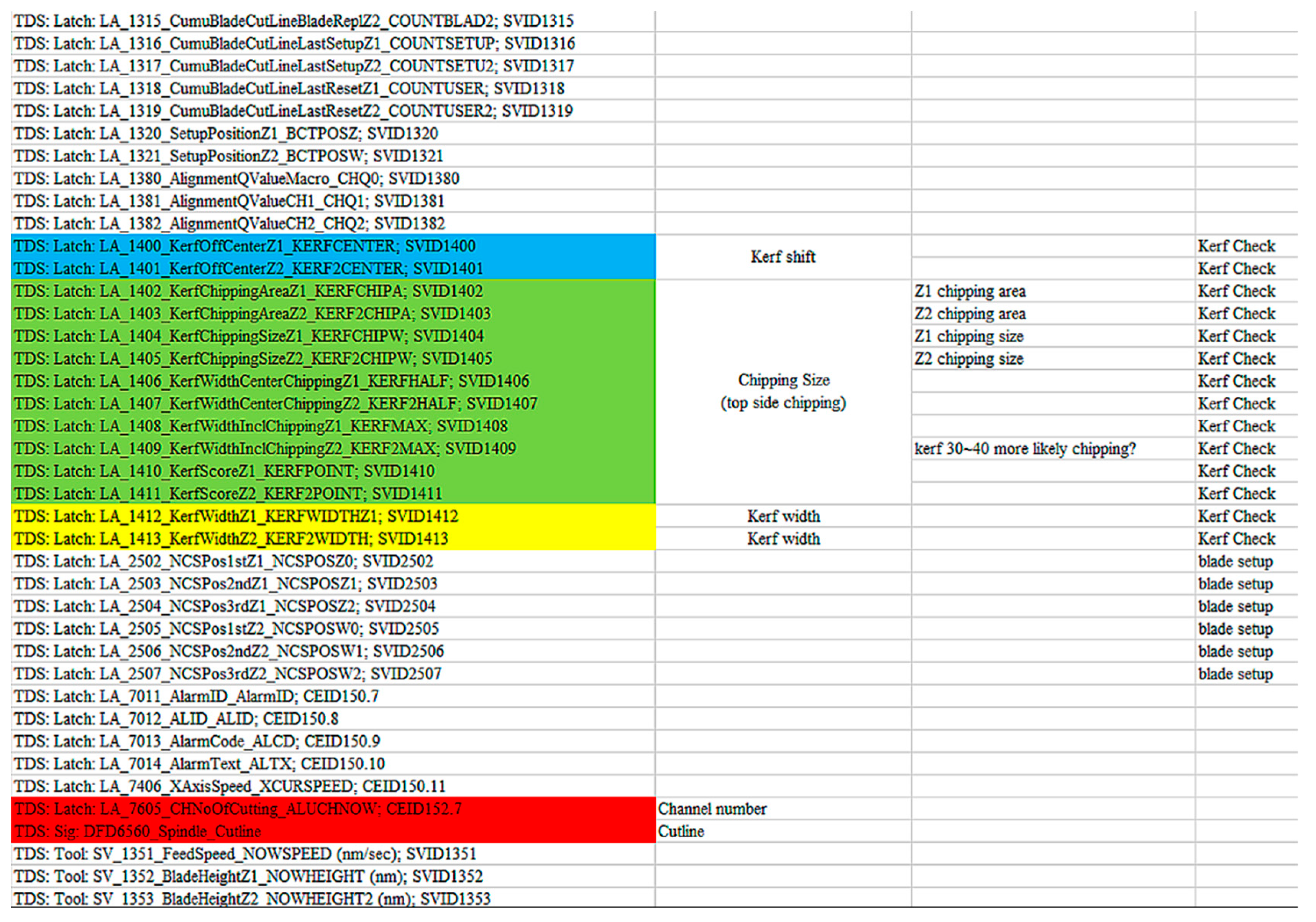
According to the channel number and cutline, on-site operators think of the following important signal listed in a summary table for the different parameter code groups with a color blue, green, yellow, and red background, as shown in Figure 10. Figure 11 displays the parameter code as a string with a color red and blue background, which can query the data about various wafer grinding parameters corresponding to the wafer chipping position.
- (2)
- We installed the Python programming execution environment of Anaconda3 on Windows 10. Moreover, installing relevant data analysis packages such as Pandas, Numpy, Scikit-learn, Tensorflow, and Keras is still necessary. In addition, Python programming requires setting up packages such as Matplotlib and Pyplot for drawing visual graphics.
- (3)
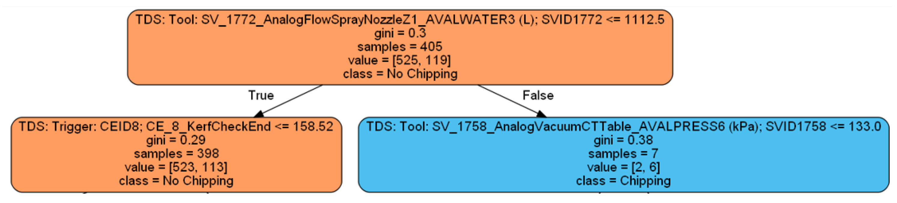
- We have checked the judgment conditions of each key parameter in different decision trees, as shown in Figure 12. According to the judgment conditions of each node in the decision tree, we can observe different parameter values, which are the normal and chipping situations. According to the parameter values within the judgment conditions, it is possible to know which key parameters will have a greater impact on the occurrence of wafer chipping. In Figure 12, we found that the parameter SVID_1772 of the node in the decision tree has eight data values greater than 1112.5, of which the machines judged six to be chipping situations. Therefore, the key grinding parameter SVID_1772 has an important influence on whether wafer chipping occurs. In random forest estimation, we can filter the ten key parameters extracted from the importance analysis to the eight most important parameters for the next step. These key parameters are SpindleCurrent_Z1, SpindleCurrent_Z2, SVID_1772, SVID_1773, SVID_1775, SVID_1752, SVID_1753, and SVID_1785. Among them, Information Gain can evaluate the chaos evaluation index of the decision tree in Equation (8), where p is the probability that the condition is true, and q is the probability that the condition is false. When Entropy in Equation (9) is 0, it means that the data types classified in this area of the data are all consistent.
- (4)
- Meanwhile, we use the decision tree presented in the previous step (3) to explore how every grinding parameter’s importance can affect the wafer grinding result and determine which ones are the key grinding parameters. After that, we conduct the correlation analysis on these parameters, as shown in Figure 13. We found that the spindle current of two blades will significantly impact the yield of wafer grinding and then continue to pick out the other eight key grinding parameters. The random forest method can estimate the possible chipping phenomenon caused by these ten key grinding parameters. We have imported these ten key grinding parameters into the random forest, and the pairings can achieve 87% accuracy when estimating wafer chipping coverage areas of less than 30% of the wafer surface area. This estimation accuracy is higher than the 78% accuracy using all grinding parameters.
- (5)
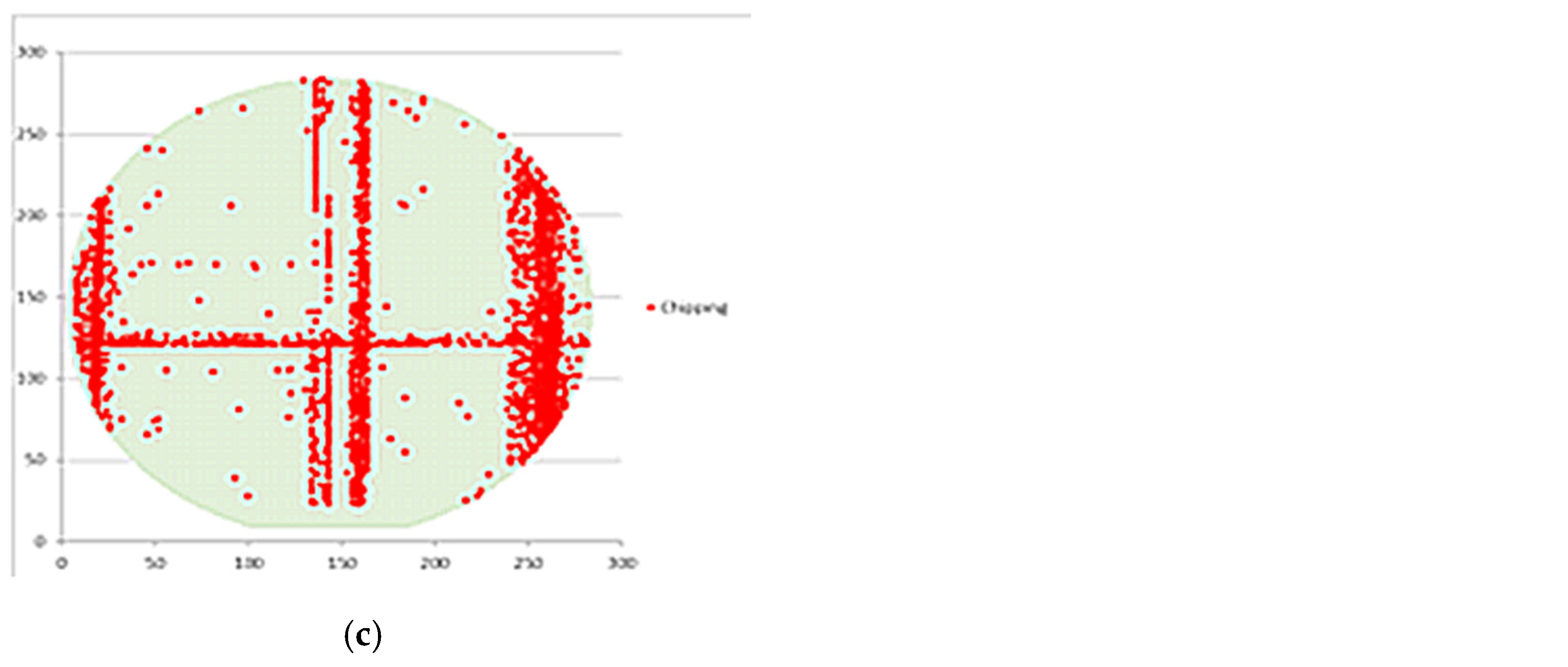
- First, this study used a time series analysis to check the data distribution relationship between the normal situation and the occurrence of chipping. This check goes through many wafers to examine whether normal behavior exists in the data distribution relationship where red dots represent the occurrence of wafer chipping, as shown in Figure 14. When examining the wafer grinding process, we found that the parameter SVID_1752 of the cleaning gas emission on the wafer may chip when its pressure is lower than 586. In addition, we also found that if the air pressure of the parameter SVID_1753 fluctuates too much, it is easy to cause this chipping phenomenon, as shown in Figure 15.
- (6)
- This study has tried three methods for correlation analysis: Pearson, Spearman, and Kendall tau. Technically speaking, we chose Kendall tau, which is more suitable for working on non-linear data distribution. It will make a comparison based on sorting the respective sequence sizes in the two parameters. First, it will make a comparison based on sorting the respective sequence sizes in the two parameters. Then, Equation (10) can compute the Kendall tau correlation, where represents the total number of concordant pairs and stands for the total number of discordant pairs. Finally, we can visualize the result of the correlation matrix among the various parameters, as shown in Figure 16. We found that the kerf width, kerf displacement, and the length of each blade between the two blades had a correlation between 0.45 and 0.74. According to the correlation between the parameters mentioned above, people can judge a considerable degree of mutual influence between the blades.
- (7)
- This study standardized eight key grinding parameters mentioned above for data preprocessing and then aggregated these key parameters into a high-dimensional parameter vector. Furthermore, dimensionality reduction can condense this parameter vector to a one-dimensional constant value as an index. Finally, we apply the heat map analysis to this index, explaining the trend in potential chipping. This study has introduced two vector dimensionality reduction methods, PCA and Barnes-Hut t-SNE, as shown in Figure 17 and Figure 18. In Figure 17 and Figure 18, the x-axis in (a) represents the current cutline map with starting cutline number 0. Since the leftmost part of the wafer map in (d) is drawn from coordinate 3, the x-axis of the wafer map in (d) corresponding to the cutline map in (a) is the cutline number + 3. The x-axis of the cutline map in (c) corresponding to the wafer map in (d) is 81, the cutline number. Compared with PCA, Barnes-Hut t-SNE is more pronounced concerning the degree of change in the value of dimensionality reduction. This discovery indicates that the Barnes-Hut t-SNE data changes are more sensitive than PCA when chipping occurs. Therefore, this study selected the Barnes-Hut t-SNE dimensionality reduction to better judge chipping occurrence than PCA.
- (8)
- To increase the amount of training data before training DD-BLSTM, we will partition the data set of wafer chipping area of less than 30% into four groups: 10%, 10~15%, 15~20%, and 20~30%, and then perform average pooling to smooth the four sampled data picked up from each group at the same corresponding sequence in order to obtain a new datum, increasing the amount of training data. The dimensionality-reduced data called index has been imported into the DD-BLSTM model to make an inference for predicting potential large-scale chipping, as shown in Figure 5. We can use it to check how effective the key grinding parameters are in predicting the occurrence of wafer chipping. In addition, we can also verify whether a decisive influence exists on the occurrence of wafer chipping. Figure 19 shows that the DD-BLSTM model with index inputs can get a loss (error) of 0.1126 during the training phase. After the test phase, we can use the trained model to predict the occurrence of wafer chipping in the other wafer grinding processes, as shown in Figure 20. In Figure 20, we found that in the early stage of the wafer grinding process, this study imported the index to the DD-BLSTM model, which can accurately predict the index that will happen shortly. In such a way, it is possible to determine whether chipping will occur soon. Therefore, we can use the predicted index to detect whether the wafer chipping has occurred or, based on the trend in the potential chipping, tell people that chipping may occur soon.
4. Experiment Results and Discussion
This section first describes the specifications of the production machines used for wafer grinding. It then gives the results before and after tuning key grinding parameters to improve the effect of wafer grinding. Finally, after implementing dimensionality reduction using PCA and Barnes-Hut t-SNE methods individually to get their respective condensed information (i.e., an index), we can import this information (an index) into the BLSTM model to predict the likely chipping in the wafer grinding process, and make the comparison of the accuracy of the chipping prediction with/without tuning key grinding parameters in the wafer grinding process.
4.1. Experiment Setting
In Figure 21, the production machine is DISCO DS6560, which was used in the experiments of wafer grinding in this section. The hardware specifications are shown in detail and are listed in Table 1.
The recipe of packages is available for applications used in this section, as listed in Table 2. The packages of Pandas and Numpy can perform data preprocessing. The machine learning suite Scikit-learn provides two dimensionality reduction methods, PCA and Barnes-Hut t-SNE. We used Tensorflow and Keras to build the deep learning model. Finally, Matplotlib or Pyplot package can show the experimental results visually.
4.2. Experimental Design
4.2.1. Settings for Parameter Dimensionality Reduction
As mentioned above, the importance analysis yielded seven important parameters of wafer grinding, including a spindle current, three kinds of water flow, and three kinds of cleaning gas emissions. We aggregated them into a seven-dimensional vector. Then, this study uses the Barnes-Hut t-SNE method to reduce the vector dimension. People can set either the exact or barnes_hut option in the t-SNE manual, and this experiment sets the barnes_hut option to speed up the calculation of dimensionality reduction. This setting can complete the calculation with time complexity O(n[log]n). This is faster than the other one with O(n2). This parameter setting is suitable for the application of wafer grinding in practice. The dimensionality reduction has generated 223,990 data concerning the key parameters from 112 pieces of wafer grinding. Since the amount of data is relatively large, we set the parameter perplexity to 50. This study chooses the parameter of early_exaggeration with the default 4.0 and the parameter learning_rate of 1000. If the cost function value of KL divergence increases in early training, people can consider reducing the parameters learning_rate and early_exaggeration. We set 1000 for the parameter n_iter, which represents the maximum number of iterations during optimization, and 30 for the parameter n_iter_without_progress, which means that the iteration will stop if there is no progress after 30 iterations. This study set 0.2 as the parameter angle, which is the relaxation degree of fault tolerance. However, the time required for calculation can be increased and can make the calculation result more accurate.
4.2.2. Settings for Chipping Prediction
A single LSTM model has three layers and a total of 640 neurons, as shown in Figure 5. In Figure 5, the activation function σ is the sigmoid function, and is the hyperbolic tangent. The loss function is a mean-square error (MSE) and the optimizer adaptive moment estimation (Adam). If the accuracy rate does not increase after ten training rounds, the process will terminate the training. We set the batch size to 128 and the maximum number of training rounds to 150. This study set the parameter return_sequences to true, which can return short-term output results between multiple units. In the training phase, we had a training data set with 167,993 signals used to train the BLSTM model, which collected the front-end grinding signals and their corresponding backend grinding signals of 82 different wafers.
Consequently, the trained model can infer the backend grinding signals according to the front-end grinding signals. We picked up 10% of the training data set in the training phase as validation to verify the training results. In the test phase, we tested the trained DD-BLSTM model using the test data set that had a total of 55,997 pairs of front-end grinding signals and their corresponding backend grinding signals out of 30 different wafers.
4.3. Experimental Results
4.3.1. Chipping Prediction Accuracy
After implementing dimensionality reduction methods PCA and Barnes-Hut t-SNE to obtain the condensed information (i.e., an index), we trained a DD-BLSTM model of index prediction for wafer chipping with different dimensionality reduction methods, PCA and Barnes-Hut t-SNE, as shown in Figure 22. Then, we imported this index into the trained DD-BLSTM model to predict the likely chipping of wafer grinding and compared the predicting accuracy between different dimensionality reductions, as listed in Table 3.
In Table 3, the fab has categorized the samples of wafer chipping obtained from the machines during the wafer grinding process into two classes. The first class is that the chipping area of a single wafer is less than 30%, and the second class is more significant than 30%. The ratio of the number of samples from the former to the number of samples from the latter is 11:1. First, we have trained the prediction model DD-BLSTM using the collected samples of wafer chipping mentioned above to obtain the trained model accordingly. As a result, the prediction accuracy of the first class of wafer chipping is higher than that of the second class of wafer chipping by 9.02% in the test. Next, according to the wafer-chipping samples mentioned above, the chipping data have scattered a non-linear distribution. Therefore, the prediction accuracy using the Barnes-Hut t-SNE dimensionality reduction method will be higher than that of the PCA dimensionality reduction method by 17.02% in the test.
Table 4 compares the prediction accuracy among models using Barnes-Hut t-SNE dimensionality reduction. In Table 4, DD-BLSTM has achieved the best accuracy in both Classes. LSTM has the worst prediction accuracy in Class I, whereas Auto Encoder has the worst prediction accuracy in Class II.
Table 5 compares prediction accuracy with different dimensionality reductions using the Barnes-Hut t-SNE method after dimensionality. After the test, the case of 1-dimensional can obtain the best prediction accuracy.
4.3.2. Wafer Grinding Results
In wafer grinding, the nonlinear Barnes-Hut t-SNE reduces the dimensionality of the input vector to obtain the condensed information (i.e., an index) and this information is imported into the DD-BLSTM model to predict the likely chipping. This study proposed two approaches in the experiments. In the first approach, the production machine runs wafer grinding without tuning the key grinding parameters. In the second approach, the production machine can tune the key grinding parameters in a timely way during the grinding process and check whether or not it can effectively control large-scale wafer chipping. In wafer grinding, the probability of wafer chipping will gradually increase due to the rapid wear of the blade, as shown in Figure 23. In Figure 23, when grinding at the third wafer, the production machine must change the blades to alleviate the occurrence of large-scale chipping.
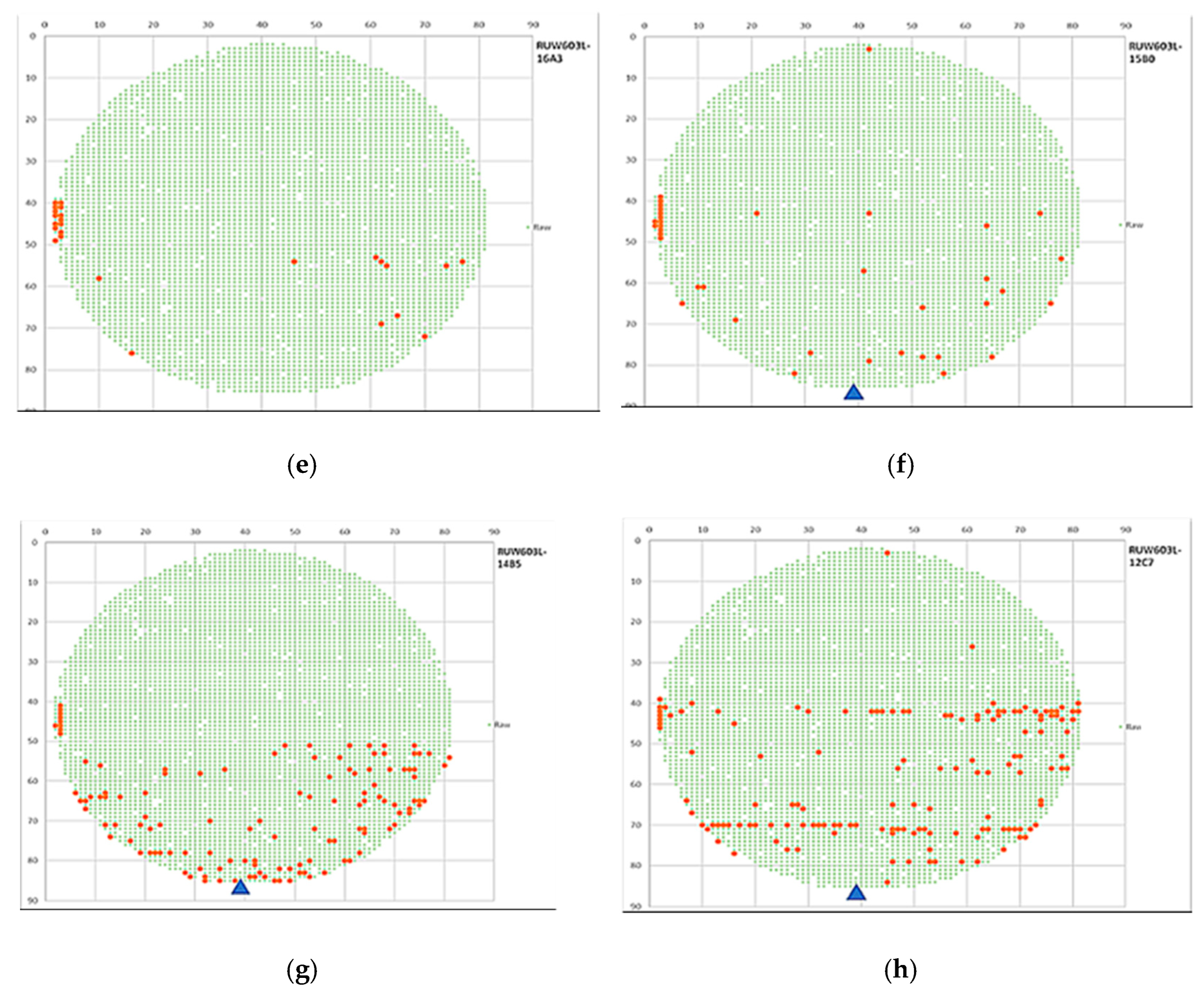
In contrast, in the second approach, the production machine can tune the key grinding parameters to stabilize the spindle current, monitor the water flow rate, and clean the gas emissions at any time during the grinding process. Consequently, it can defer the deterioration of the blades, and thus the speed of wafer chipping gets slower, as shown in Figure 24. Compared with the first approach, the second can extend the useful life of the blade to grind more wafers, as listed in Table 6. As a result, the proposed approach can significantly improve wafer grinding yield and thus reduce the loss of manufacturing costs.
4.4. Discussion
This study used the random forest method to estimate the chipping phenomenon during wafer grinding, which can effectively explore the important grinding parameters. This paper has shown that the prediction accuracy of a wafer chipping coverage area of less than 30% can be as high as 87% of the wafer surface area. However, the random forest can only estimate most of the errors after the wafer chipping has occurred and cannot do it in the process of chipping. The sensitivity of chipping detection and prediction during wafer grinding is poor. Moreover, if we have tested a wafer with around 50% chipping coverage area, the estimation accuracy of the random forest will drop to 52%. After chipping, the estimation misclassified them as normal, and most estimation errors arose. The estimation process only can pick out a few chippings successfully. The random forest needs to observe the judgment conditions of nodes, focus several key nodes on judging whether or not it could cause chipping, and then screen out the key grinding parameters.
In addition, the paper [32] compares the detection ability of outliers between the LSTM model and the BLSTM model. The wafer chipping frequency will increase over time because the blade will continue to wear while grinding until the machine replaces it. The article [19] uses the LSTM model to provide better prediction accuracy for data with temporal causality. With the same parameter settings, the BLSTM model will achieve better prediction accuracy than the LSTM model. Furthermore, this study has proposed a DD-BLSTM to replace a BLSTM model to get the best chipping detection and prediction performance.
The limitation of this experiment is that the earlier wafer grinding machines used in this experiment and the data generated by the machines are somewhat lacking. Therefore, it is necessary to mark the area where the chipping has occurred manually. Then, according to the manually marked areas, we must find each piece of chipping data individually, which requires a lot of workforce to aggregate the data. In addition, if the chipping coverage area accounts for more than 70% of the wafer surface area and the other extreme conditions, the currently trained model cannot provide the prediction accuracy as well as we expected. Fabs will not allow the worn blade to be in this lousy situation without replacing the blade during wafer grinding. Nevertheless, the currently trained model can successfully run chipping detection in the wafer grinding process.
5. Conclusions
Fabs have adopted many methods to adjust the parameters of the wafer grinding. However, simple regression cannot wholly analyze large-scale wafer backside wall chipping because the wafer grinding process encounters many problems, such as collected data missing, data showing a non-linear distribution, and correlated hidden parameters lost. The main contribution of this study was to propose a novel approach to solving this problem. We adopted importance analysis to find the key grinding parameters, used the Barnes-Hut t-SNE method to reduce the dimensionality of the key grinding parameters, and established a DD-BLSTM model to predict the occurrence of large-scale chipping. The objective of this study is to adjust the key grinding parameters in time to reduce the occurrence of large-scale wafer chipping. As a result, the proposed approach can significantly increase the yield of wafer grinding and reduce the loss of wafer manufacturing costs.
The experiments operated with the earlier machines, and the machines generated various signals that were not as detailed and precise as the latest machines. Suppose we can obtain a new machine that can capture more parameters, such as audio or video signals. In that case, we can effectively establish a powerful prediction model to improve accuracy. In future work, if a new machine can make the output data more complete, the assistance of visual algorithms and related packages through the program can automatically mark the abnormal values generated from the machines. As mentioned above, collecting data will save a lot regarding workforce and time.
Author Contributions
B.R.C. and H.-Y.M. conceived and designed the experiments; H.-F.T. collected the experimental dataset and proofread the paper; B.R.C. wrote the paper. All authors have read and agreed to the published version of the manuscript.
Funding
This research was funded by the Ministry of Science and Technology, Taiwan, MOST 111-2221-E-390-012 and MOST 111-2622-E-390-001, and The APC was funded by the Ministry of Science and Technology, Taiwan.
Data Availability Statement
The Sample Program.zip data used to support this study’s findings are available as follows: https://drive.google.com/file/d/1SPfMmKr43bQDvxU5iY9O1jpab7H-GUGn/view?usp=sharing (accessed on 19 June 2022).
Acknowledgments
This paper is supported and granted by the Ministry of Science and Technology, Taiwan (MOST 111-2622-E-390-001 and MOST 110-2622-E-390-001).
Conflicts of Interest
The authors declare no conflict of interest.
References
- Rosa-Zurera, M.; Jarabo-Amores, P.; Lopez-Ferreras, F.; Sanz-Gonzalez, J.L. Comparative analysis of importance sampling techniques to estimate error functions for training neural networks. In Proceedings of the IEEE/SP 13th Workshop on Statistical Signal Processing, Bordeaux, France, 17–20 July 2005; pp. 121–126. [Google Scholar] [CrossRef]
- Onda, H. Framework for wafer level control APC model. In Proceedings of the 2011 e-Manufacturing & Design Collaboration Symposium & International Symposium on Semiconductor Manufacturing (eMDC & ISSM), Hsinchu, Taiwan, 5–6 September 2011; pp. 1–10. Available online: http://resolver.scholarsportal.info/resolve/1523553x/v2011inone/1_ffwlcam.xml (accessed on 21 October 2022).
- Khokhar, M.S.; Cheng, K.; Ayoub, M.; Zakria; Eric, L.K. Multi-Dimension Projection for Non-Linear Data Via Spearman Correlation Analysis (MD-SCA). In Proceedings of the 2019 8th International Conference on Information and Communication Technologies (ICICT), Karachi, Pakistan, 16–17 November 2019; pp. 14–18. [Google Scholar] [CrossRef]
- Dong, Y.-Q. Value Ranges of Spearman’s Rho and Kendall’s Tau of a Class of Copulas. In Proceedings of the 2010 International Conference on Computational and Information Sciences, Chengdu, China, 17–19 December 2010; pp. 182–185. [Google Scholar] [CrossRef]
- Zhang, Z.; Yang, X. Constructing Copulas on the Parabolic Boundary of Kendall’s Tau-Spearman’s Rho Region. In Proceedings of the 2010 First ACIS International Symposium on Cryptography, and Network Security, Data Mining and Knowledge Discovery, E-Commerce and Its Applications, and Embedded Systems, Qinhuangdao, China, 23–24 October 2010; pp. 324–327. [Google Scholar] [CrossRef]
- Sangwan, A.; Zhu, W.; Ahmad, M.O. Design and Performance Analysis of Bayesian, Neyman–Pearson, and Competitive Neyman–Pearson Voice Activity Detectors. IEEE Trans. Signal Process. 2007, 55, 4341–4353. [Google Scholar] [CrossRef]
- Zhang, Q.T.; Song, S.H. Model Selection and Estimation for Lognormal Sums in Pearson’s Framework. In Proceedings of the 2006 IEEE 63rd Vehicular Technology Conference, Melbourne, VIC, Australia, 7–10 May 2006; pp. 2823–2827. [Google Scholar] [CrossRef]
- Jiao, Y.; Vert, J. The Kendall and Mallows Kernels for Permutations. IEEE Trans. Pattern Anal. Mach. Intell. 2018, 40, 1755–1769. [Google Scholar] [CrossRef] [PubMed] [Green Version]
- Zhang, Z.; Wang, H. Within Wafer & Wafer to Wafer Thickness Uniformity Controllable Study on ILD-CMP Via Polishing Pad’s Physical Property Analysis and Linear Interval Feedback APC’s Implementation. In Proceedings of the 2019 China Semiconductor Technology International Conference (CSTIC), Shanghai, China, 18–19 March 2019; pp. 1–3. [Google Scholar] [CrossRef]
- Gang, D.; He, Y.; Shao, X. Anomaly Detection and Analysis of FDC Data. In Proceedings of the 2021 5th IEEE Electron Devices Technology & Manufacturing Conference (EDTM), Chengdu, China, 8–11 April 2021; pp. 1–3. [Google Scholar] [CrossRef]
- Thiry, L.; Zhao, H.; Hassenforder, M. Categorical Models for BigData. In Proceedings of the 2018 IEEE International Congress on Big Data (BigData Congress), San Francisco, CA, USA, 2–7 July 2018; pp. 272–275. [Google Scholar] [CrossRef]
- Yamaki, S.; Seki, S.; Sugita, N.; Yoshizawa, M. Performance Evaluation of Cross Correlation Functions Based on Correlation Filters. In Proceedings of the 2021 20th International Symposium on Communications and Information Technologies (ISCIT), Tottori, Japan, 19–22 October 2021; pp. 145–149. [Google Scholar] [CrossRef]
- Garibo-Morante, A.A.; Tellez, F.O. Univariate and Multivariate Time Series Modeling using a Harmonic Decomposition Methodology. IEEE Lat. Am. Trans. 2022, 20, 372–378. [Google Scholar] [CrossRef]
- Kang, S.; Cho, S.; An, D.; Rim, J. Using Wafer Map Features to Better Predict Die-Level Failures in Final Test. IEEE Trans. Semicond. Manuf. 2015, 28, 431–437. [Google Scholar] [CrossRef]
- Schelthoff, K.; Jacobi, C.; Schlosser, E.; Plohmann, D.; Janus, M.; Furmans, K. Feature Selection for Waiting Time Predictions in Semiconductor Wafer Fabs. IEEE Trans. Semicond. Manuf. 2022, 35, 546–555. [Google Scholar] [CrossRef]
- Li, K.S.-M.; Jiang, X.-H.; Chen, L.L.-Y.; Wang, S.-Y.; Huang, A.Y.-A.; Chen, J.E.; Liang, H.S.; Hsu, C.-L. Wafer Defect Pattern Labeling and Recognition Using Semi-Supervised Learning. IEEE Trans. Semicond. Manuf. 2022, 35, 291–299. [Google Scholar] [CrossRef]
- Tsuda, T.; Inoue, S.; Kayahara, A.; Imai, S.-i.; Tanaka, T.; Sato, N.; Yasuda, S. Advanced Semiconductor Manufacturing Using Big Data. IEEE Trans. Semicond. Manuf. 2015, 28, 229–235. [Google Scholar] [CrossRef]
- Fan, S.-K.S.; Hsu, C.-Y.; Tsai, D.-M.; He, F.; Cheng, C.-C. Data-Driven Approach for Fault Detection and Diagnostic in Semiconductor Manufacturing. IEEE Trans. Autom. Sci. Eng. 2020, 17, 1925–1936. [Google Scholar] [CrossRef]
- Sunny, M.A.I.; Maswood, M.M.S.; Alharbi, A.G. Deep Learning-Based Stock Price Prediction Using LSTM and Bi-Directional LSTM Model. In Proceedings of the 2020 2nd Novel Intelligent and Leading Emerging Sciences Conference (NILES), Giza, Egypt, 24–26 October 2020; pp. 87–92. [Google Scholar] [CrossRef]
- Yang, S. Research on Network Behavior Anomaly Analysis Based on Bidirectional LSTM. In Proceedings of the 2019 IEEE 3rd Information Technology, Networking, Electronic and Automation Control Conference (ITNEC), Chengdu, China, 15–17 March 2019; pp. 798–802. [Google Scholar] [CrossRef]
- Liu, D.; Wang, J.; Shang, S.; Han, P. MSDR: Multi-Step Dependency Relation Networks for Spatial-Temporal Forecasting. In Proceedings of the 28th ACM SIGKDD Conference on Knowledge Discovery and Data Mining, Washington, DC, USA, 14–18 August 2022. [Google Scholar] [CrossRef]
- Ou, J.; Sun, J.; Zhu, Y.; Jin, H.; Zhang, F.; Huang, J.; Wang, X. STP-TrellisNets: Spatial-Temporal Parallel TrellisNets for Metro Station Passenger Flow Prediction. In Proceedings of the 29th ACM International Conference on Information and Knowledge Management, Virtual Event, 19–23 October 2020. [Google Scholar] [CrossRef]
- Deng, S.; Rangwala, H.; Ning, Y. Robust Event Forecasting with Spatiotemporal Confounder Learning. In Proceedings of the 28th ACM SIGKDD Conference on Knowledge Discovery and Data Mining, Washington, DC, USA, 14–18 August 2022. [Google Scholar] [CrossRef]
- Yumeng, C.; Yinglan, F. Research on PCA Data Dimension Reduction Algorithm Based on Entropy Weight Method. In Proceedings of the 2020 2nd International Conference on Machine Learning, Big Data and Business Intelligence (MLBDBI), Taiyuan, China, 23–25 October 2020; pp. 392–396. [Google Scholar] [CrossRef]
- White, M.T.; Jeon, S. Using t-SNE to explore Misclassification. In Proceedings of the 2019 IEEE MIT Undergraduate Research Technology Conference (URTC), Cambridge, MA, USA, 11–13 October 2019; pp. 1–4. [Google Scholar] [CrossRef]
- Meyer, B.H.; Pozo, A.T.R.; Zola, W.M.N. Improving Barnes-Hut t-SNE Scalability in GPU with Efficient Memory Access Strategies. In Proceedings of the 2020 International Joint Conference on Neural Networks (IJCNN), Glasgow, UK, 19–24 July 2020; pp. 1–8. [Google Scholar] [CrossRef]
- Xue, D.; Zhong, C.; Zhang, E.; Jiang, W.; Zhang, C. Die chipping FDC development at wafer saw process. In Proceedings of the 2021 22nd International Conference on Electronic Packaging Technology (ICEPT), Xiamen, China, 14–17 September 2021; pp. 1–2. [Google Scholar] [CrossRef]
- Zeng, Y.; Lou, Z. The New PCA for Dynamic and Non-Gaussian Processes. In Proceedings of the 2020 Chinese Automation Congress (CAC), Shanghai, China, 6–8 November 2020; pp. 935–938. [Google Scholar] [CrossRef]
- Xia, Z.; Chen, Y.; Xu, C. Multiview PCA: A Methodology of Feature Extraction and Dimension Reduction for High-Order Data. IEEE Trans. Cybern. 2022, 52, 11068–11080. [Google Scholar] [CrossRef] [PubMed]
- Liu, D.; Guo, T.; Chen, M. Fault Detection Based on Modified t-SNE. In Proceedings of the 2019 CAA Symposium on Fault Detection, Supervision and Safety for Technical Processes (SAFEPROCESS), Xiamen, China, 5–7 July 2019; pp. 269–273. [Google Scholar] [CrossRef]
- Chatzimparmpas, A.; Martins, R.M.; Kerren, A. t-viSNE: Interactive Assessment and Interpretation of t-SNE Projections. IEEE Trans. Vis. Comput. Graph. 2020, 26, 2696–2714. [Google Scholar] [CrossRef] [PubMed]
- Aparna, R.; Chitralekha, C.K.; Chaudhari, S. Comparative study of CNN, VGG16 with LSTM and VGG16 with Bidirectional LSTM using kitchen activity dataset. In Proceedings of the 2021 Fifth International Conference on I-SMAC (IoT in Social, Mobile, Analytics and Cloud) (I-SMAC), Palladam, India, 11–13 November 2021; pp. 836–843. [Google Scholar] [CrossRef]
Figure 1.
Fault Detection and Classification (FDC).

Figure 2.
LSTM Architecture.

Figure 3.
BLSTM flowchart.

Figure 4.
Barnes-Hut t-SNE dimensionality reduction flowchart.

Figure 5.
BLSTM architecture.

Figure 6.
New information from the average pooling of equal-sample partitions.

Figure 7.
Execution flow.

Figure 8.
A sample wafer chipping.

Figure 9.
Cutline, channel number, and blade number of each coordinate.

Figure 10.
Parameter title and its related information.

Figure 11.
Wafer grinding signals.

Figure 12.
Condition of a node in the decision tree.

Figure 13.
Important parameters in wafer grinding.

Figure 14.
(a) mode CH1 in the wafer ID TR7VC470W12C2; (b) mode CH2 in the wafer ID TR7VC470W12C2; (c) mode CH1 in the wafer ID TR7W1101W04F7; (d) mode CH2 in the wafer ID TR7W1101W04F7.
Figure 14.
(a) mode CH1 in the wafer ID TR7VC470W12C2; (b) mode CH2 in the wafer ID TR7VC470W12C2; (c) mode CH1 in the wafer ID TR7W1101W04F7; (d) mode CH2 in the wafer ID TR7W1101W04F7.

Figure 15.
Time series of parameter SVID_1753 in the wafer ID TR7W1101W04F7.

Figure 16.
Correlation coefficient matrix.

Figure 17.
Heat map after PCA dimensionality reduction where (a) Heat map of kerf Z1; (b) Cutting Sequence; (c) Heat map of kerf Z2 in which arrows represent sawing direction; (d) Wafer chipping coordinate of ID: RUW603L_13C2 in CH2 in which a triangle symbol represents the kerf Z1 stopped location.

Figure 18.
Heat map after Barnes-Hut t-SNE dimensionality reduction where (a) Heat map of kerf Z1; (b) Cutting Sequence; (c) Heat map of kerf Z2 in which arrows represent sawing direction; (d) Wafer chipping coordinate of ID: RUW603L_13C2 in CH2 in which a blue triangle represents the kerf Z1 stopped location.


Figure 19.
Loss and accuracy in training phase of DD-BLSTM model.

Figure 20.
DD-BLSTM prediction of index changes and chipping discovery where the brown rectangle represents the occurrence of predicted chipping and true chipping simultaneously.
Figure 20.
DD-BLSTM prediction of index changes and chipping discovery where the brown rectangle represents the occurrence of predicted chipping and true chipping simultaneously.

Figure 21.
Production machine DISCO DS6560.

Figure 22.
Training a DD-BLSTM model of index prediction.

Figure 23.
Wafer chipping distribution without tuning parameters where (a) grinding of the 1st wafer; (b) grinding of the 2nd wafer; (c) grinding of the 3rd wafer.
Figure 23.
Wafer chipping distribution without tuning parameters where (a) grinding of the 1st wafer; (b) grinding of the 2nd wafer; (c) grinding of the 3rd wafer.


Figure 24.
Wafer chipping distribution with tuning parameters where (a) grinding of the 1st wafer; (b) grinding of the 2nd wafer; (c) grinding of the 3rd wafer; (d) grinding of the 4th wafer; (e) grinding of the 5th wafer; (f) grinding of the 6th wafer; (g) grinding of the 7th wafer; (h) grinding of the 8th wafer. A blue triangle represents the kerf Z1 stopped location.


Table 1.
Specifications of DISCO DS6560.
| Specification | Unit | High Speed (Option) with 1.8 kW | ||
|---|---|---|---|---|
| Z1 | Z2 | |||
| Max. workpiece size | mm | Φ300 | ||
| X-axis | Cutting range | mm | 310 | |
| Cutting speed | mm/s | 0.1~1000 | ||
| Y1·Y2-axis | Cutting range | mm | 310 | |
| Index step | mm | 0.0001 | ||
| Positioning accuracy | mm | Within 0.002/310 (Single error) Within 0.002/5 | ||
| Z-axis | Max. stroke | mm | 14.2 (For Φ2 inch blade) | |
| Moving resolution | mm | 0.00005 | ||
| Repeatability accuracy | mm | 0.001 | ||
| θ-axis | Max. rotating angle | deg | 380 | |
| Spindle | Rated torque | N·m | 0.29 | 0.19 |
| Revolution speed range | min−1 | 6000~60,000 | 20,000~80,000 | |
| Machine dimensions (W × D × H) | mm | 1240 × 1550 × 1960 | 81 mm convex (left side) | |
| Machine weight | kg | Approx. 1640 | ||
Table 2.
Recipe of Packages.
| Software | Version |
|---|---|
| Anaconda® Individual Edition | 4.10.3 |
| Jupyter Notebook | 4.3.1 |
| Tensorflow | 2.6.2 |
| Keras | 2.6.0 |
| Pandas | 1.1.5 |
| Numpy | 1.19.5 |
| Matplotlib | 3.3.4 |
| Pyplot | 5.5.0 |
| Scikit-learn | 0.23.2 |
Table 3.
Accuracy of chipping prediction using different dimensionality reductions.
| Dimensionality Reduction | PCA | Barnes-Hut t-SNE | |
|---|---|---|---|
| Chipping Area of a Wafer | |||
| Class I: Less than 30% | 0.7612 | 0.9314 | |
| Class II: More than 30% | 0.5236 | 0.8412 | |
Table 4.
The accuracy of prediction models using Barnes-Hut t-SNE.
| Models | LSTM | AutoEncoder | BLSTM | DD-BLSTM | |
|---|---|---|---|---|---|
| Wafer Chipping Area | |||||
| Class I: Less than 30% | 0.8122 | 0.8611 | 0.9234 | 0.9314 | |
| Class II: More than 30% | 0.6413 | 0.5219 | 0.8216 | 0.8412 | |
Table 5.
Comparison of the prediction accuracy with different dimensionality reduction.
| Model and Class | DD-BLSTM | ||
|---|---|---|---|
| Dimensionality | Class I | Class II | |
| 1-dimensional | 0.9314 | 0.8412 | |
| 2-dimensional | 0.9223 | 0.8212 | |
| 3-dimensional | 0.9121 | 0.8303 | |
| 4-dimensional | 0.9222 | 0.8083 | |
| 5-dimensional | 0.9313 | 0.8155 | |
| 6-dimensional | 0.8771 | 0.7798 | |
| 7-dimensional | 0.8511 | 0.7421 | |
| 8-dimensional | 0.8365 | 0.7254 | |
Table 6.
Wafer grinding using different approaches.
| Method | Original Approach | Proposed Approach | |
|---|---|---|---|
| Attribute | |||
| Number of grinding wafers needed to change kerf immediately | 3 | 8 | |
| Backside wall chipping distributed | Whole wafer | The bottom half of a wafer | |
Publisher’s Note: MDPI stays neutral with regard to jurisdictional claims in published maps and institutional affiliations. |
© 2022 by the authors. Licensee MDPI, Basel, Switzerland. This article is an open access article distributed under the terms and conditions of the Creative Commons Attribution (CC BY) license (https://creativecommons.org/licenses/by/4.0/).
Share and Cite
MDPI and ACS Style
Chang, B.R.; Tsai, H.-F.; Mo, H.-Y. Detection and Prediction of Chipping in Wafer Grinding Based on Dicing Signal. Mathematics 2022, 10, 4631. https://0-doi-org.brum.beds.ac.uk/10.3390/math10244631
AMA Style
Chang BR, Tsai H-F, Mo H-Y. Detection and Prediction of Chipping in Wafer Grinding Based on Dicing Signal. Mathematics. 2022; 10(24):4631. https://0-doi-org.brum.beds.ac.uk/10.3390/math10244631
Chicago/Turabian StyleChang, Bao Rong, Hsiu-Fen Tsai, and Hsiang-Yu Mo. 2022. "Detection and Prediction of Chipping in Wafer Grinding Based on Dicing Signal" Mathematics 10, no. 24: 4631. https://0-doi-org.brum.beds.ac.uk/10.3390/math10244631
Note that from the first issue of 2016, this journal uses article numbers instead of page numbers. See further details here.