Article

Note on the Numerical Solutions of Unsteady Flow and Heat Transfer of Jeffrey Fluid Past Stretching Sheet with Soret and Dufour Effects

1
Department of Mathematics, College of Science and Humanities in Al-Kharj, Prince Sattam bin Abdulaziz University, Al-Kharj 11942, Saudi Arabia
2
Department of Basic Engineering Science, Faculty of Engineering, Menoufia University, Shebin El-Kom 32511, Egypt
3
Department of Mathematics, COMSATS University, Islamabad 45550, Pakistan
4
Department of Mathematics, University of Sargodha, Sargodha 40100, Pakistan
5
Department of Mathematics, Faculty of Science, Aswan University, Aswan 81528, Egypt
*
Author to whom correspondence should be addressed.
Submission received: 1 November 2022 / Revised: 24 November 2022 / Accepted: 25 November 2022 / Published: 7 December 2022

Abstract

:
A numerical investigation of unsteady boundary layer flow with heat and mass transfer of non-Newtonian fluid model, namely, Jeffrey fluid subject, to the significance of Soret and Dufour effects is carried out by using the local nonsimilarity method and homotopy analysis method. An excellent agreement in the numerical results obtained by both methods is observed and we establish a new mathematical approach to obtain the solutions of unsteady-state flow with heat and mass transfer phenomenons. Similarity transformation is applied to governing boundary layer partial differential equations to obtain the set of self-similar, nondimensional partial differential equations. Graphical results for different emerging parameters are discussed. The dimensionless quantities of interest skin friction coefficient, Sherwood number, and Nusselt number are discussed through tabulated results. The main novelty of the current work is that the average residual error of the m t h -order approximation of the OHAM scheme for steady-state solution is decreased for higher-order approximation. Further, a rapid development of the boundary layer thickness with the increasing values of dimensionless time τ is observed. It is noted that for large values of τ , the steady state in the flow pattern is gained. It is worth mentioning that the magnitude of Sherwood number is increased with the increasing values of Schmidt number S c and Dufour number D f . The magnitude of local Nisselt number is increased for the increasing values of Soret number, S r .
MSC:
76D05; 76D10

1. Introduction

The significance of boundary layer flow of Newtonian/non-Newtonian fluids past a stretching surface has gained the attention of many researchers due to their applications in science and engineering, e.g., polymer extrusion, food processing, and many others. With this understanding, first, we focus on the work of the community engaged in this field. Initially, the boundary layer flow of viscous fluid was discussed by Crane [1] theoretically. The case of heat and mass transfer analysis with suction and blowing was studied by Gupta and Gupta [2]. Magnetohydrodynamic flow and heat transfer of viscous fluid past stretching sheet was discussed by Chakrabarti and Gupta [3] numerically. The uniqueness of solutions of the Navier–Stokes fluid past a stretching sheet was determined by Mcleod and Rajagopal [4] in detail. The numerical solutions of boundary layer flow of viscous fluid past stretching plate were simulated by Liao [5], and they presented the obtained results graphically as well as in tabular form. Magnetohydrodynamic flow due to vertical stretching sheet with heat transfer was studied by Ishak et al. [6] theoretically. Further, the MHD free convection flow past vertical stretching plate under the influence of heat generation and viscous dissipation was studied by Khaleque and Samad [7]. The stagnation point flow of upper convected Maxwell fluid past stretching sheet with melting heat transfer was studied by Hayat et al. [8]. Further extension in this model for similar flow for third-grade fluid with viscous dissipation was discussed by Hayat et al. [9]. Three-dimensional flow of Oldroyd-B fluid over a bidirectional stretching sheet with surface temperature and surface heat flux generation was studied by Hayat et al. [10].
The real-world formulation of emerging phenomenons is not adequate when the constitutive relations for viscous fluid are applied. Therefore, to completely describe the true behavior, we must take into consideration non-Newtonian fluid models which are more adequate to describe the nature of fluid flow. A large variety of non-Newtonian fluid models have been studied for boundary layer flows of non-Newtonian fluids, among which is the Jeffrey fluid model. This fluid model is capable of describing the characteristics of relaxation and retardation times of the non-Newtonian fluids. Analysis of an endoscope and magnetic field on the peristalsis involving Jeffrey fluid were carried out by Hayat et al. [11]. Magnetohydrodynamic peristaltic flow of Jeffery fluid through finite length of cylindrical tube was studied by Tripathi et al. [12]. Further, the MHD peristaltic flow of a Jeffrey fluid under the influence of slip and heat transfer in inclined asymmetric porous channel was studied by Das [13], and heat source or sink effects past stretching sheet for Jeffrey fluid were discussed by Qasim [14]. Three-dimensional stretched flow of Jeffrey fluid under the influence of variable thermal conductivity and thermal radiation was discussed by Hayat et al. [15]. Lifting of a Jeffrey fluid on a vertical belt under influence of magnetic field and wall slip conditions was discussed by Farooq et al. [16]. The time-dependent analysis of flow and heat transfer of Jeffrey fluid along stretching sheet was carried out by Hayat et al. [17]. The stagnation-point flow of Jeffrey fluid under the effects of melting heat transfer and mass transfer with Soret and Dufour effects was studied by Hayat et al. [18]. Moreover, the Jeffrey fluid flow between two torsionally oscillating disks was discussed by Reddy et al. [19].
When heat and mass transfer occur simultaneously between two mediums, the relations between the fluxes and the driving potentials are significant in nature. Experimental studies showed that an energy flux can be generated not only by temperature gradients but by composition of gradient as well, which can be given by the Fick’s laws of diffusion. This type of energy flux is known as Dufour or diffusion-thermo effect. In a similar manner, we also have mass fluxes being created by temperature gradient, which can be given by the Fourier’s laws of heat conduction, and this phenomenon is known as Soret or thermal-diffusion. The energy and concentration generation due to Dufour and Soret effects are comparatively small in magnitude as compared to other effects; however, these effects are significantly important for the light molecular weight substances. Forced and natural convection boundary layer flow with the significance of Soret and Dufour effects was studied by Abreu et al. [20]. Soret and Dufour effects with the inclusion of variable wall temperature and concentration are discussed by Cheng [21]. The MHD Hiemenz flow and mass transfer with Soret and Dufour effects through porous medium along the stretching sheet were studied by Addel-Rahman [22]. Mixed convection flow of second-grade fluid subject to Hall and ion-slip currents with Soret and Dufour effects were studied by Hayat and Nawaz [23]. Three-dimensional flow in a viscoelastic fluid past stretching surface with significance of Soret and Dufour effects was studied by Hayat et al. [24]. The natural convection heat and mass transfer flow past a horizontal surface in porous medium with variable viscosity with significance of Soret and Dufour effects was investigated by Moorthy et al. [25]. Axisymmetric flow of a Jeffery fluid over a stretching surface with significance of Newtonian heating along with thermal-diffusion and diffusion-thermo effects was studied by Awais et al. [26].
Homotopy analysis method was developed by Liao [27]. The homotopy analysis method has been successfully applied to many highly nonlinear problems in the last decade; some of them are [5,8,9,10,15,17,18,23,24,26]. The development in the homotopy analysis method was made by many researchers. One of them is the optimal homotopy analysis method (OHAM), in which the convergence of homotopy solution is determined by the optimization of convergence control parameters against the residual error, as mentioned in [28,29]. The local nonsimilarity method was introduced by Sparrow and Yu [30], and the solutions of nonsimilar equations arising in mixed convection flow was discussed. The numerical analysis of the local nonsimilarity method at third level of truncation was carried out by Yu and Sparrow [31], and Rabadi and Dweik applied this method in the mixed convective flow with flux [32]. Massoudi discussed the local nonsimilarity solutions for the flow of a non-Newtonian fluid over a wedge [33]. Yian and Norsarahaida [34] studied vertical free convection boundary layers flow using local nonsimilarity method. Mushtaq et al. [35] studied the mixed convection flow of second-grade subject to vertical stretching flat surface with variable surface temperature. Recently, Kairi et al. [36] conducted a numerical study on the influence of viscous dissipation and thermo-diffusion subjected to double-diffusive convection over a vertical cone in a non-Darcy porous medium saturated by a non-Newtonian fluid with variable heat and mass fluxes. Sardar et al. [37] investigated the local nonsimilar solutions in the convective flow of Carreau fluid with the inclusion of MHD and radiative heat transfer. Swarajya and Rao [38] applied this method to study variations in drag and heat transfer at a vertical plate due to steady flow of a colloidal suspension of the nanofluid. RamReddy et al. [39] studied the significance of nonlinear Boussinesq approximation on natural convective flow with the method of local nonsimilarity approach. Keeping in view the above literature review, our current problem deals with the unsteady flow and heat transfer of Jeffrey fluid past a stretching sheet with the inclusion of Soret and Dufour effects. As far as our approach and knowledge, the local nonsimilarity method has never been applied to unsteady flow phenomenons so far, so we are the first to use this method in conjunction with the homotopy analysis method and also carry out a numerical compression for both approaches.

2. Mathematical Formulation

We consider the unsteady incompressible bidirectional boundary layer flow of the Jeffrey fluid with constant viscosity μ and density ρ past a stretching sheet. Initially, the fluid and the plate are at rest. The flow is induced by the sudden stretching of the sheet with constant velocity u w ( x ) = c x , where c is a positive (stretching sheet) constant. The stretching sheet is raised to a temperature T w , and T is the embedded temperature of the fluid such that ( T w > T ) , as shown in Figure 1. The conservation equations for the proposed model take the following forms:
· V = 0 ,
ρ D V D t = d i v τ 1 + ρ F ,
ρ C p D T D t = k 2 T + Φ + J ,
D C D t = D 2 C + R c .
where V is the velocity, ρ is density, T is the temperature, C p is the specific heat and constant pressure, k is thermal conductivity of the fluid, Φ is the viscous dissipation, J is the Dufour effect, C is the concentration of diffusion species, D is the diffusion coefficient, R c is the Soret effect, D D t is the material derivative, F is the body for force, and τ 1 is the Cauchy stress tensor. For incompressible Jeffrey fluid, this tensor is given by
τ 1 = p I + S ,
where p is pressure and the extra stress tensor S is given by
S = μ 1 + λ 1 A 1 + λ 2 D A 1 D t ,
where μ is the viscosity of the fluid, λ 2 is the ratio of relaxation and retardation time, and λ 1 is retardation time, respectively. A 1 is the first Rivlin–Erickson tensor, given by
A 1 = ( V ) + ( V ) ,
where ⋆ denotes the transpose. The heat flux J , also known as known as Dufour or diffusion-thermo effect, can be given by Frick’s law of diffusion, as follows:
J = ρ D K t C s 2 C ,
where C s is the specific heat capacity of the solid surface, K T is the thermal diffusion ratio, and R c is the concentration flux generated by the temperature gradient, known as Soret or thermo-diffusion effect, given by Fourier’s law of heat conduction:
R c = q . A = D k T 2 T T m .
where T m is the mean temperature of the fluid. We assume that viscous dissipation Φ is insignificant and we consider the thermal and radiative heat transfer along with the Soret and Dufour effect in this unsteady fluid flow. It is also assumed that all the thermal properties are taken as constant. Body forces are negligible and the pressure p is constant for the fluid flow. The governing boundary layer equations under the standard Prandtl boundary layer approximations are given by
u x + v y = 0 ,
u t + u u x + v u y = ν 1 + λ 2 2 u y 2 + λ 1 3 u y 2 t + u 3 u x y 2 u x 2 u y 2 + u y 2 u x y + v 3 u y 3 ,
T t + u T x + v T y = k ρ C P 2 T y 2 + 16 σ T 3 3 ρ C P k 2 T y 2 + D k T C S 2 C y 2 ,
C t + u C x + v C y = D 2 C y 2 + D k T T m 2 T y 2 ,
subject to boundary conditions
t 0 : u = 0 , v = 0 , T = T , C = C for any x , y t > 0 : u = u w ( x ) = a x , v = 0 , T = T w , C = C w at y = 0 , u 0 , v 0 , T T , C C as y ,
where σ is the Stefan–Boltzmann constant and k is Rosseland mean absorption coefficient. The expressions for skin friction coefficient C f x , local Nusselt number N u x , and local Sherwood number S h are given by
C f x = τ w 1 / 2 ρ u w ( x ) 2 , N u x = x q w k ( T w T ) , S h x = x j w D C w C ,
where the wall skin friction τ w , wall heat flux q w , and mass flux j w are given by
τ w = μ 1 + λ 2 u y + λ 1 u 2 u y x + 2 u y t + v 2 u y 2 y = 0 , q w = k + 16 σ T 3 3 k T y y = 0 , j w = D C y y = 0 .
We introduce the similarity variables of the form
η = a ν ξ y , u = a x f ( η , ξ ) , v = a ν ξ f ( η , ξ ) , ξ = 1 exp [ τ ] , τ = a t , θ ( η , ξ ) = T T T w T , ϕ ( η , ξ ) = C C C w C ,
Using (17) in Equations (10)–(13) along the initial and boundary conditions (14), we obtain the following transformed system of self-similar partial differential equations:
{ ξ β ( 1 ξ ) } f + 1 + λ 2 ξ ( 1 ξ ) ( η 2 f ξ f ξ ) ξ 2 ( f 2 f f ) + β ξ ( 1 ξ ) f ξ η 2 ( 1 ξ ) f i v + ξ f 2 f f = 0 ,
θ + Pr e f f 1 ξ η 2 θ ξ θ ξ + Pr e f f ξ f θ + Pr e f f D f ϕ = 0 ,
ϕ + S c 1 ξ η 2 ϕ ξ ϕ ξ + S c ξ f ϕ + S c S r θ = 0 ,
with the initial and boundary conditions
f ( 0 , ξ ) = 0 , f ( 0 , ξ ) = 1 , θ ( 0 , ξ ) = 1 , ϕ ( 0 , ξ ) = 1 , f ( , ξ ) = 0 , θ ( , ξ ) = 0 , ϕ ( , ξ ) = 0 ,
where
β = a λ 1 , Pr = ρ C P υ k , R d = 4 σ T 3 k k , Pr e f f = Pr 1 + 4 3 R d , D f = D k T ( C w C ) C P C S ( T w T ) , S c = υ D , S r = D k T ( T w T ) T m ( C w C ) ,
where prime denotes the derivatives with respect to η , β is the Deborah number, P r is Prandtl number, R d is the radiation parameter, Pr e f f is the effective Prandtl number, D f is the Dufour number, S c is the Schmidt number, and S r is the Soret number. The similarity expression for skin friction coefficient C f x , local Nusselt number N u x , and local Sherwood number S h x are given by using (17) in Equations (15) and (16). We have
1 / 2 ξ 1 2 R e x 1 / 2 C f = 1 1 + λ 2 1 + β f 0 , ξ + β 1 ξ f 0 , ξ ξ 1 2 ξ f 0 , ξ , ξ 1 2 R e x 1 / 2 N u x = 1 + 4 3 R d θ 0 , ξ , ξ 1 2 R e x 1 / 2 S h = ϕ 0 , ξ ,
where R e x = a x 2 / ν = U w x / ν is the local Reynolds number.

3. Steady-State Flow

To obtain the steady-state flow problem we input ξ = 1 in Equations (18)–(20), and we obtain
f + 1 + λ 2 ( f 2 + f f ) + β f 2 f f = 0 ,
θ + Pr e f f f θ + Pr e f f D f ϕ = 0 ,
ϕ + S c f ϕ + S c S r θ = 0 ,
with the conditions
f ( 0 ) = 0 , f ( 0 ) = 1 , θ ( 0 ) = 1 , ϕ ( 0 ) = 1 , f ( ) = 0 , θ ( ) = 0 , ϕ ( ) = 0 .
It is important to note that the exact solution of Equation (24), subject to boundary conditions (27), has the form
f η = 1 e m η m ; m = 1 + λ 2 1 + β .
Substituting the expression of f ( η ) from Equation (28) into Equations (25) and (26), the resulting differential equation can be solved numerically by the symbolic computation software Mathematica version 13.1, Wolfram Research, Champaign, Illinois.

4. Solution Methodology

4.1. Local Nonsimilarity Method

4.1.1. First Level of Truncation

At the first level of truncation, the terms containing ξ ( . ) ξ in Equations (18)–(20) are neglected under the assumption that the terms involving ξ are small [37]. This is particularly true when ξ < < 1 . Thus, the terms with ξ ( . ) ξ of Equations (18)–(20) are neglected to obtain the following system of equations:
{ ξ β ( 1 ξ ) } f + 1 + λ 2 ξ ( 1 ξ ) ( η 2 f ) ξ 2 ( f 2 f f ) + β ξ f 2 f f i v η 2 ( 1 ξ ) f i v = 0 ,
θ + Pr e f f 1 ξ η 2 θ + Pr e f f ξ f θ + Pr e f f D f ϕ = 0 ,
ϕ + S c 1 ξ η 2 ϕ + S c ξ f ϕ + S c S r θ = 0 ,
with the initial and boundary conditions
f ( 0 , ξ ) = 0 , f ( 0 , ξ ) = 1 , θ ( 0 , ξ ) = 1 , ϕ ( 0 , ξ ) = 1 , f ( , ξ ) = 0 , θ ( , ξ ) = 0 , ϕ ( , ξ ) = 0 ,
It can be seen that Equations (29)–(31) can be treated as a system of ordinary differential equations for the functions f ( η ) and θ ( η ) and ϕ ( η ) with ξ as a parameter.

4.1.2. Second Level of Truncation

To find the higher level of truncation, we introduce the following new functions:
g ( η , ξ ) = f ξ , h ( η , ξ ) = f ξ , j ( η , ξ ) = f ξ ,
At the second level, the governing equations, Equations (18)–(20), for the function f ( η , ξ ) , θ ( η , ξ ) , and ϕ ( η , ξ ) , respectively, are retained intact, and are as follows:
{ ξ β ( 1 ξ ) } f + 1 + λ 2 ξ ( 1 ξ ) ( η 2 f ξ g ) ξ 2 ( f 2 f f ) + β ξ ( 1 ξ ) g η 2 ( 1 ξ ) f i v + ξ f 2 f f = 0 ,
θ + P r e f f 1 ξ η 2 θ ξ h + P r e f f ξ f θ + P r e f f D f ϕ = 0 ,
ϕ + S c 1 ξ η 2 ϕ ξ j + S c ξ f ϕ + S c S r θ = 0 ,
with the initial and boundary conditions
f ( 0 , ξ ) = 0 , f ( 0 , ξ ) = 1 , θ ( 0 , ξ ) = 1 , ϕ ( 0 , ξ ) = 1 , f ( , ξ ) = 0 , θ ( , ξ ) = 0 , ϕ ( , ξ ) = 0 ,
To derive the subsidiary equations for g ( η ; ξ ) , h ( η ; ξ ) , and j ( η ; ξ ) and their boundary conditions, we take the derivatives of Equations (34)–(36) with respect to ξ . Thus, we obtain
( 1 + β ) f + ξ ( 1 β ) g + 1 + λ 2 { ( 1 2 ξ ) η 2 f + ( 3 ξ 2 2 ξ ) g + ξ ( 1 ξ ) η 2 g 2 ξ f 2 f f ξ 2 2 f g f g f g } + β η 2 f ( i v ) η 2 ( 1 ξ ) g ( i v ) + f 2 f f i v + ξ 2 f g g f ( i v ) f g ( i v ) = 0 ,
h + P r e f f ( 2 ξ 1 ) h η 2 θ + ( 1 ξ ) η 2 h + P r e f f f θ + ξ g θ + f h + P r e f f D f j = 0
j + S c ( 2 ξ 1 ) j η 2 ϕ + ( 1 ξ ) η 2 j + S c f ϕ + ξ g ϕ + f j + S c S r h = 0
subject to boundary conditions
g ( 0 , ξ ) = 0 , g ( 0 , ξ ) = 0 , h ( 0 , ξ ) = 0 , j ( 0 , ξ ) = 0 , g ( , ξ ) = 0 , h ( , ξ ) = 0 , j ( , ξ ) = 0 .
At this level of truncation, the terms g ξ , h ξ , and j ξ and their derivative terms with respect to η are neglected. Considering the present scheme, solutions of the equations for the functions f ( η ; ξ ) , θ ( η ; ξ ) , ϕ ( η ; ξ ) , g ( η ; ξ ) , h ( η ; ξ ) , and j ( η ; ξ ) are obtained using the MatLab built-in package b v p 4 c .

4.2. Homotopy Analysis Method

We select the initial guesses and the linear operator for the homotopy analysis method (HAM) and the optimal homotopy analysis method (OHAM) as
f 0 η = 1 e η , θ 0 ( η ) = e η , ϕ 0 ( η ) = e η ,
L f f = f f , L θ f = f f , L ϕ f = f f ,
where L f , L θ , and L ϕ satisfy the following properties:
L f A 1 + A 2 e η + A 3 e η = 0 , L θ A 4 e η + A 5 e η = 0 , L ϕ A 6 e η + A 7 e η = 0 ,
where A i ( i = 1 - - 7 ) are the arbitrary constants and have to be determined later.

5. Results and Discussion

The system of self-similar partial differential Equations (18)–(20) subject to the boundary conditions (21) is solved directly by the homotopy analysis method, whereas local nonsimilarity is applied at the second level of truncation. The system of self-similar ordinary differential Equations (34)–(36) subject to the boundary conditions (37) for the functions f, θ , and ϕ and Equations (38)–(40) subject to the boundary conditions (41) for the g, h, and j with ξ as a parameter is solved numerically. Table 1 shows the numerical comparison of the values of f ( 0 , ξ ) , θ ( 0 , ξ ) , and ϕ ( 0 , ξ ) obtained by the 15th-order homotopy analysis method, and with the values of convergence control parameters f = 0.70 , θ = 1.2 , and ϕ = 0.16 and the numerical solution of system of ordinary differential equations with the help of computer software MatLab by considering arbitrary values of the emerging parameters. We observe a significant agreement in the numerical results obtained by both mathematical approaches.
For ξ = 1 , the steady-state flow given by Equations (24)–(26), we first obtain the optimized values of the convergence control parameter by using Module G e t O p t i V a r [ m ] of the MATHEMATICA package B V P H 2.0 . Table 2 shows the corresponding values of convergence control parameters at different order of homotopy approximations. Table 3 shows the average residual error of mth-order approximation of OHAM steady-state solution, and we observe a decrease in the residual error for higher-order approximations. Table 4 shows the convergence of steady-state approximations of OHAM solutions with optimized values of convergence control parameters as f = 1.3 , θ = 1.0 , and ϕ = 1.0 .

5.1. Analysis of Solutions

5.1.1. Transient-State Solutions

Three-dimensional plots are shown in Figure 2, Figure 3 and Figure 4; these surfaces are generated for dimensionless time unsteady parameter ξ [ 0 , 1 ] and for η [ 0 , ] . The growth of solution is observed with increase in ξ , and the effect of stretch vanishes for large values of η .
Figure 5, Figure 6 and Figure 7 show the behavior of the dimensionless time τ on the development of boundary layer thickness of velocity profile f ( η , ξ ) , temperature profile θ ( η , ξ ) , and concentration profile ϕ ( η , ξ ) , respectively. We observe a rapid development of boundary layer thickness with increases in dimensionless time τ and gain the steady-state flow as τ . Figure 8 and Figure 9 show the influence of the β and λ 2 on velocity profile, respectively, and it is found that the velocity profile is increasing function of β and decreasing function of λ 2 . Figure 10 and Figure 11 show the influence of the D f and Pr e f f on temperature profile, respectively, and it is found that the temperature profile is increasing function of D f and decreasing function of Pr e f f . Figure 12 and Figure 13 show the influence of the S c and S r on concentration profile, respectively, and it is found that the velocity profile is decreasing function of S c and increasing function of S r .

5.1.2. Steady-State Solutions

In Figure 14 and Figure 15, we compare the exact solutions of f ( η ) and the analytical series solution derived by OHAM . It is found that the derived series solution agrees with the exact solution for different values of β and λ 2 . Moreover, the small values of Deborah number β are associated with the liquid-like behavior of the matter, and for the large values of Deborah number β , solid-like behavior is associated. Keeping this fact in mind, we plotted the graphs with only small values of Deborah number β . We observed that the velocity profile f ( η ) is an increasing function with the increase in Deborah number β . On the other hand, the velocity profile f ( η ) is a decreasing function of increasing relaxation time λ 2 .  Figure 16 and Figure 17 show that the OHAM solution of θ ( η ) agrees with the numerical solutions obtained by MATHEMATICA. As we know, for the small values of effective Prandtl number Pr e f f the fluid is highly conductive. Physically, if Pr e f f increases, the thermal diffusivity decreases and this effect leads to the decrease in thermal energy transfer ability; thus, we have a decrease in thermal boundary layer thickness. Figure 17 shows the influence of effective Prandtl number Pr e f f on the temperature profile θ ( η ) , and, as expected, with increase in Pr e f f , we observe a decrease in temperature and thermal boundary layer thickness. Figure 16 represents the effect of Dufour number D f on the temperature profile and thermal boundary layer thickness; it is found that the temperature is an increasing function of the Dufour number D f and we observe increased thermal boundary layer thickness with increasing Dufour number D f . Figure 18 and Figure 19 show the effect of Schmidt number S c on the concentration profile and it is found that the concentration profile is the decreasing function of the Schmidt number S c . There is aneffect of Soret number S r on the concentration profile, and it is found that the concentration profile is the rapidly increasing function of the Soret number S r .

5.2. Dimensionless Numbers Analysis

The combined effect of Deborah number β and λ 2 on the skin friction coefficient is shown in Table 5. Similar behavior is obtained by HAM and LNS methods, and results indicate that the magnitude of the skin friction coefficient is a decreasing function of β and increasing function of λ 2 . Table 6 shows the numerical values of local Nusselt number and Sherwood number given by (15) with different values of emerging parameters with ξ = 0.5 and R d = 0.1 . The results indicate that the magnitude of local Nusselt number and Sherwood number increases with increase in Deborah number β and decreases with increase in λ 2 , respectively. The magnitude of local Nusselt number increases with increase in effective Prandtl number Pr e f f , whereas Sherwood number is a decreasing function of this parameter. The magnitude of local Nusselt number decreases with increase in Dufour number D f , ; in other words, an increase in D f decreases the temperature. On the other hand, magnitude of Sherwood number increases with increase in D f . The magnitude of local Nusselt number decreases with increase in Schmidt number S c , ; in other words, an increase in S c decreases the temperature. On the other hand, magnitude of Sherwood number increases with increase in S c . The magnitude of local Nusselt number increases with increase in Soret number S r ; in other words, an increase in S r increases the temperature. On the other hand, magnitude of Sherwood number decreases with increase in S r .

5.3. Closing Remarks

The unsteady flow with heat and mass transfer over stretching sheet with Soret and Dufour effects is numerically studied using two different methods. The homotopy analysis method is straightforward to apply on partial differential equations but requires very long processing time at higher order of approximations, which may be considered as a disadvantage of the homotopy analysis method. On the other hand, the numerical solutions of system of ordinary differential equations at second level of truncation are easily computed with very small processing time. The results obtained by both methods are very close and the impact of emerging parameters is equivalent in both approaches. On the basis of processing time, the local nonsimilarity method is the recommended option. The influence of emerging parameters on velocity, temperature, and concentration profiles can be summarized as follows:
  • The analytical solution obtained by OHAM for the similarity equations agrees with the exact solution of steady-state velocity profile and with the numerical solution of steady-state temperature and concentration profile.
  • The velocity profile is found to be the increasing function of Deborah number β and decreasing function of λ 2 .
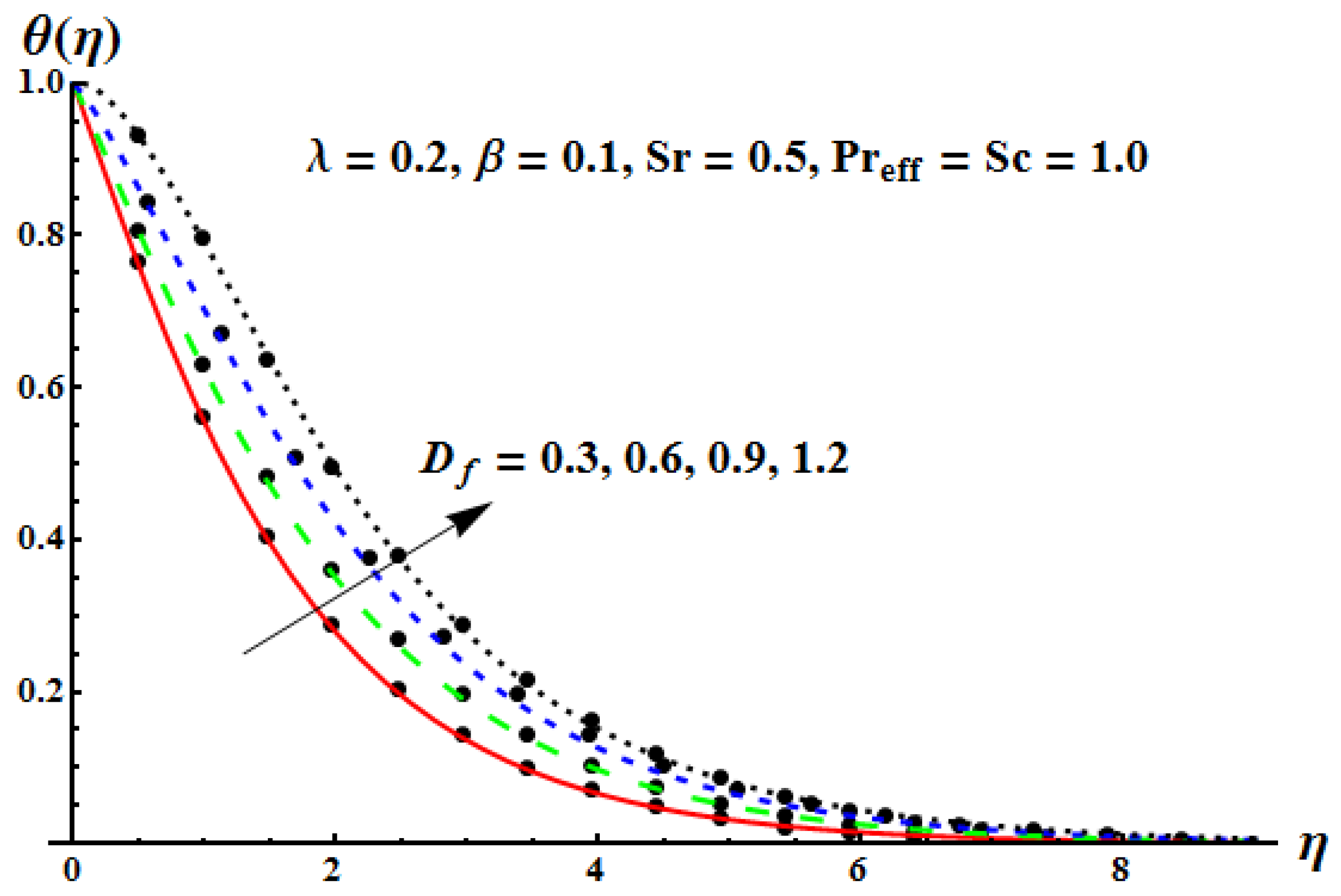
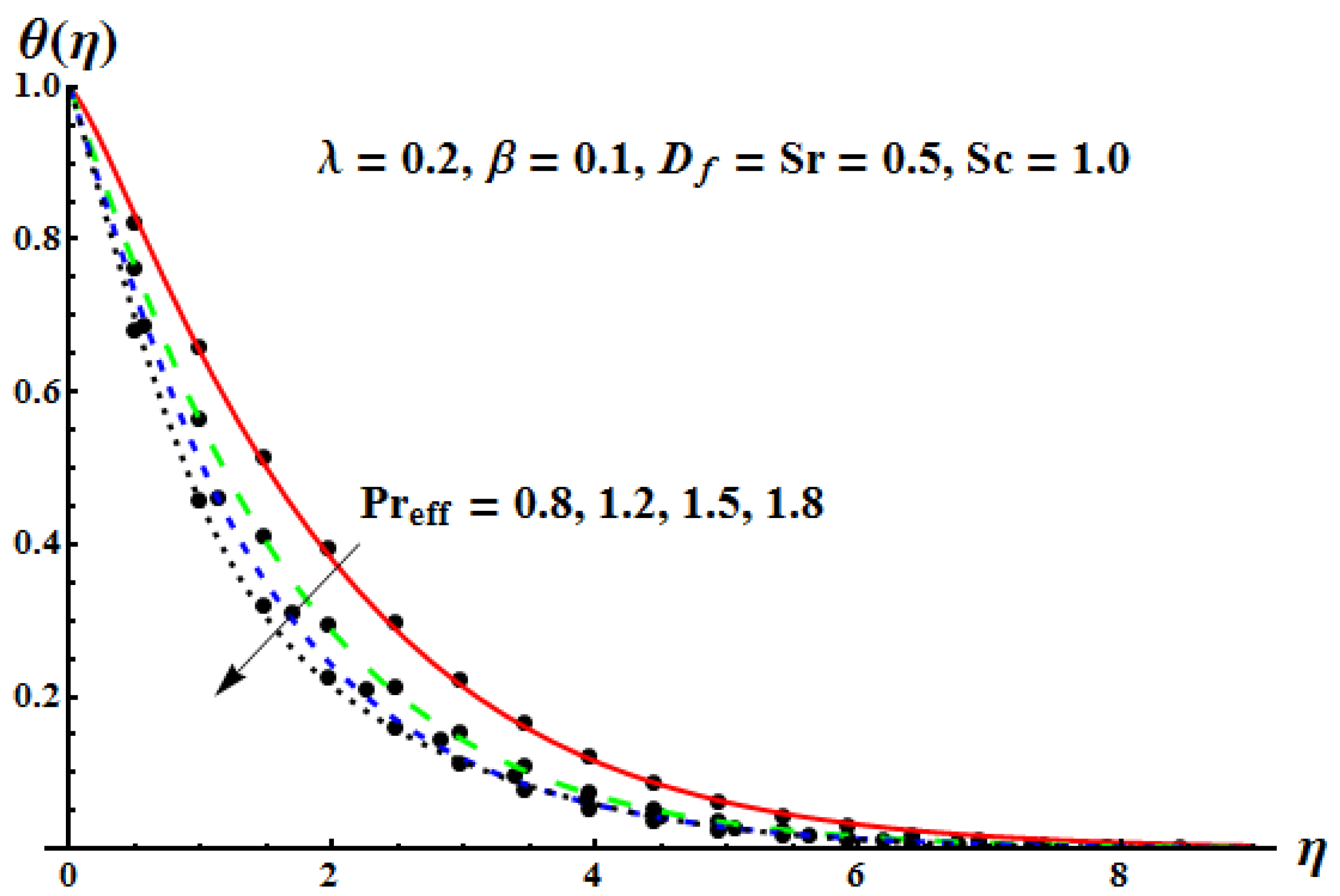
  • The temperature profile decreases with increase in effective Prandtl number Pr e f f , whereas it increases with increase in Dufour number D f . There is no significant effect of Soret number S r and Schmidt number S c on the temperature profile in the steady case.
  • The concentration profile ϕ ( η ) is an increasing function of Soret number S r and decreasing function of Schmidt number S c . There is no significant effect of effective Prandtl number Pr e f f and Dufour number D f on the concentration profile in the steady case.
  • The behavior of effective Prandtl number Pr e f f on the temperature profile is the same as the behavior of Schmidt number S c on the concentration profile. Similarly, the behavior of Dufour number D f on the temperature profile is the same as the behavior of Soret number S r on the concentration profile, in both steady and transient flow cases.
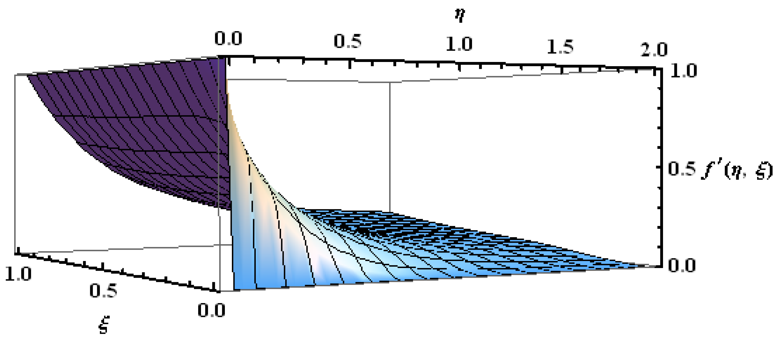
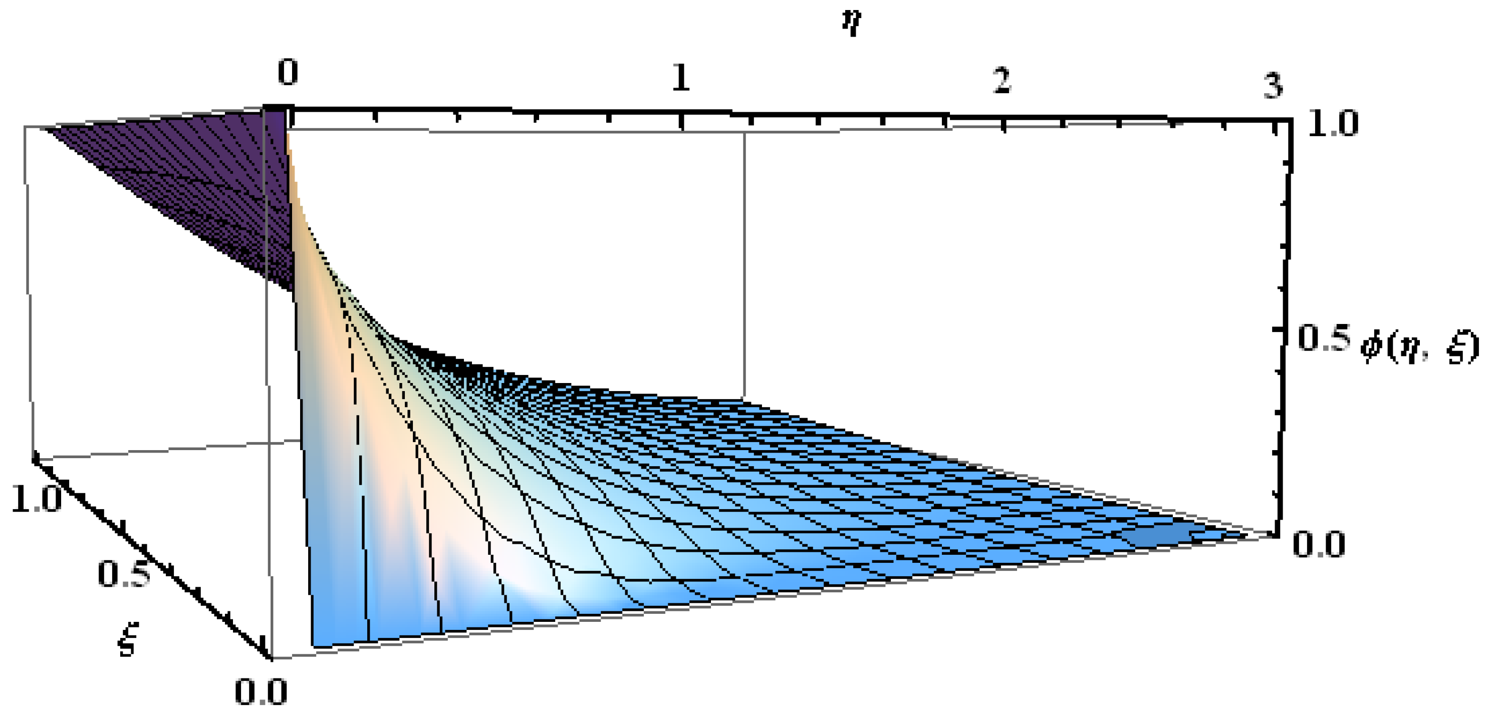
  • We observed a development of velocity, temperature, and concentration boundary layers as the dimensionless time τ increased from 0 and the boundary layers gained the steady state as dimensionless time τ .
  • The behavior of all emerging parameters for all profiles is the same as in the case of steady-state flow.
  • The skin friction coefficient is a decreasing function of β and increasing function of λ 2 , local Nusselt number is an increasing function of effective Prandtl number Pr e f f , and Sherwood number is a decreasing function of this parameter.
  • The local Nusselt number decreases with increase in Dufour number D f , and Sherwood number increases with increase in D f .
  • The local Nusselt number decreases with increase in Schmidt number S c , and Sherwood number increases with increase in S c .
  • The local Nusselt number increases with increase in Soret number S r , and Sherwood number decreases with increase in S r .

Author Contributions

Formal analysis, S.I.A.; Investigation, S.I.A. and M.A.H.; Methodology, H.A.N., M.M. and M.A.; Project administration, H.A.N.; Resources, A.M.R.; Software, M.N.; Supervision, M.A. and A.M.R.; Visualization, M.A.H.; Writing—original draft, H.A.N., M.M., M.N. and M.A.; Writing—review & editing, M.M. and M.N. All authors have read and agreed to the published version of the manuscript.

Funding

This research was funded by the Deputyship for Research & Innovation, Ministry of Education in Saudi Arabia grant number (IF2/PSAU/2022/01/22970).

Data Availability Statement

The data is generated by the authors by using FORTRAN Laher-90, no from other source.

Acknowledgments

The authors extend their appreciation to the Deputyship for Research and Innovation, Ministry of Education in Saudi Arabia for funding this research work through the project number (IF2/PSAU/2022/01/22970).

Conflicts of Interest

The authors declare no conflict of interest.

References

  1. Crane, L.J. Flow Past a Stretching Plate. J. Appl. Math. Phys. (ZAMP) 1970, 21, 60–74. [Google Scholar] [CrossRef]
  2. Gupta, P.S.; Gupta, A.S. Heat and Mass Transfer on a Stretching Sheet with Suction or Blowing. Can. J. Chem. Eng. 1977, 55, 744–746. [Google Scholar] [CrossRef]
  3. Chakrabarti, A.; Gupta, A.S. Hydromagnetic Flow and Heat Transfer Over a Stretching Sheet. Q. Appl. Math. 1979, 33, 73–78. [Google Scholar] [CrossRef] [Green Version]
  4. McLeodK, J.B.; Rajagopal, R. On the Uniqueness of Flow of a Navier-Stokes Fluid Due to a Stretching Boundary. In Analysis and Continuum Mechanics; Springer: Berlin/Heidelberg, Germany, 1987; Volume 98, pp. 385–393. [Google Scholar]
  5. Liao, S.J. A new branch of solutions of boundary-layer flows over an impermeable stretched plate. Int. J. Heat Mass Transf. 2005, 48, 2529–2539. [Google Scholar] [CrossRef]
  6. Ishak, A.; Nazar, R.; Pop, I. Hydromagnetic flow and heat transfer adjacent to a stretching vertical sheet. WSEAS Trans. Heat Mass Transf. 2008, 44, 921–927. [Google Scholar] [CrossRef]
  7. Khaleque, T.; Abdus Samad, M. Effects of Radiation, Heat Generation and Viscous Dissipation on MHD Free Convection Flow along a Stretching Sheet. Res. J. Appl. Sci. Eng. Technol. 2010, 2, 368–377. [Google Scholar]
  8. Hayat, T.; Mustafa, M.; Shehzad, S.A.; Obaidat, S. Melting heat transfer in the stagnation point flow of an upper convected Maxwell fluid past a stretching sheet. Int. J. Numer. Methods Fluids 2012, 68, 233–243. [Google Scholar] [CrossRef]
  9. Hayat, T.; Iqbal, Z.; Mustafa, M.; Hendi, A. Melting heat transfer in the stagnation point flow of third grade fluid past a stretching sheet with viscous dissipation. Therm. Sci. 2013, 17, 865–875. [Google Scholar] [CrossRef]
  10. Hayat, T.; Shehzad, S.A.; Al-Mezel, S.; Alsaedi, A. Three-dimensional flow of an Oldroyd-B fluid over a bidirectional stretching surface with prescribed surface temperature and prescribed surface heat flux. J. Hydrol. Hydromechan. 2014, 62, 117–125. [Google Scholar] [CrossRef] [Green Version]
  11. Hayat, T.; Niaz, A.; Ali, N. Effects of an endoscope and magnetic field on the peristalsis involving Jeffrey fluid. Commun. Nonlinear Sci. Numer. Simul. 2008, 13, 1581–1591. [Google Scholar] [CrossRef]
  12. Tripathi, D.; Ali, N.; Hayat, T.; Chaube, M.K.; Hendi, A.A. Peristaltic flow of MHD Jeffrey fluid through finite length cylindrical tube. Appl. Math. Mech. Engl. Ed. 2011, 32, 1231–1243. [Google Scholar] [CrossRef]
  13. Das, K. Influence of slip and heat transfer on MHD peristaltic flow of a Jeffrey fluid in an inclined asymmetric porous channel. Indian J. Math. 2012, 54, 19–45. [Google Scholar]
  14. Qasim, M. Heat and mass transfer in a Jeffrey fluid over a stretching sheet with heat source/sink. Alex. Eng. J. 2013, 52, 571–575. [Google Scholar] [CrossRef] [Green Version]
  15. Hayat, T.; Shehzad, S.A.; Alsaedi, A. Three-dimensional stretched flow of Jeffrey fluid with variable thermal conductivity and thermal radiation. Appl. Math. Mech. Engl. Ed. 2013, 34, 823–832. [Google Scholar] [CrossRef]
  16. Farooq, A.A.; Batiha, B.; Siddiqui, A.M. Lifting of a Jeffrey fluid on a vertical belt under the simultaneous effects of magnetic field and wall slip conditions. Int. J. Adv. Math. Sci. 2013, 1, 91–97. [Google Scholar] [CrossRef]
  17. Hayat, T.; Iqbal, Z.; Mustafa, M.; Alsaedi, A. Unsteady flow and heat transfer of Jeffrey fluid over a stretching sheet. Therm. Sci. 2014, 18, 1069–1078. [Google Scholar] [CrossRef]
  18. Hayat, T.; Iqbal, Z.; Mustafa, M.; Alsaedi, A. Stagnation-point flow of Jeffrey fluid with melting heat transfer and Soret and Dufour effects. Int. J. Numer. Methods Heat Fluid Flow 2014, 24, 402–418. [Google Scholar] [CrossRef]
  19. Reddy, G.B.; Sreenadh, S.; Reddy, R.H.; Kavitha, A. Flow of a Jeffrey fluid between torsionally oscillating disks. Ain Shams Eng. J. 2015, 6, 355–362. [Google Scholar] [CrossRef] [Green Version]
  20. Abreu, C.R.A.; Alfradique, M.F.; Telles, A.S. Boundary layer flows with Dufour and Soret effects: I: Forced and natural convection. Chem. Eng. Sci. 2006, 61, 4282–4289. [Google Scholar] [CrossRef]
  21. Cheng, C.Y. Soret and Dufour effects on heat and mass transfer by natural convection from a vertical truncated cone in a fluid-saturated Porous medium with variable wall temperature and concentration. Int. Commun. Heat Mass Transf. 2010, 37, 1031–1035. [Google Scholar] [CrossRef]
  22. Abdel-Rahman, G.M. Thermal-diffusion and MHD for Soret and Dufour’s effects on Hiemenz flow and mass transfer of fluid flow through porous medium onto a stretching surface. Physica B 2010, 405, 2560–2569. [Google Scholar] [CrossRef]
  23. Hayat, T.; Nawaz, M. Soret and Dufour effects on the mixed convection flow of a second grade fluid subject to Hall and ion-slip currents. Int. J. Numer. Methods Fluids 2011, 67, 1073–1099. [Google Scholar] [CrossRef]
  24. Hayat, T.; Safdar, A.; Awais, M.; Mesloub, S. Soret and Dufour effects for three-dimensional flow in a viscoelastic fluid over a stretching surface. Int. J. Heat Mass Transf. 2012, 55, 2129–2136. [Google Scholar] [CrossRef]
  25. Moorthy, M.B.K.; Kannan, T.; Senthilvadivu, K. Soret and Dufour Effects on Natural Convection Heat and Mass Transfer Flow past a Horizontal Surface in a Porous Medium with Variable Viscosity. WSEAS Trans. Heat Mass Transf. 2013, 8, 121–130. [Google Scholar]
  26. Awais, M.; Hayat, T.; Nawaz, M.; Alsaedi, A. Newtonian heating, thermal-diffusion and diffusion-thermo effects in an axisymmetric flow of a Jeffery fluid over a stretching surface. Braz. J. Chem. Eng. 2015, 32, 555–561. [Google Scholar] [CrossRef] [Green Version]
  27. Liao, S.J. Beyond Perturbation: Introduction to Homotopy Analysis Method; CRC Press LLC: Boca Raton, FL, USA, 2004. [Google Scholar]
  28. Liao, S.J. Homotopy Analysis Method in Nonlinear Differential Equations; Higher Education Press: Beijing, China, 2012. [Google Scholar]
  29. Liao, S.J. Advances in the Homotopy Analysis Method; World Scientific Publishing Co., Pte. Ltd.: Singapore, 2014. [Google Scholar]
  30. Sparrow, E.M.; Yu, H.S. Local Non-Similarity Thermal Boundary-Layer Solutions. J. Heat Transf. 1971, 93, 328–334. [Google Scholar] [CrossRef]
  31. Chen, T.S.; Sparrow, E.M. Flow and Heat Transfer Over a Flat Plate With Uniformly Distributed, Vectored Surface Mass Transfer. J. Heat Transf. 1976, 98, 674–676. [Google Scholar] [CrossRef]
  32. Rabadi, N.; Dweik, Y. Local Non-similarity Solutions for Mixed Convection Flow with Lateral Mass Flux over an Inclined Flat Plate Embedded in a Saturated Porous Medium. J. King Saud Univ.-Eng. Sci. 1995, 7, 267–286. [Google Scholar] [CrossRef]
  33. Massoudi, M. Local non-similarity solutions for the flow of a non-Newtonian fluid over a wedge. Int. J. Non-Linear Mech. 2001, 36, 961–976. [Google Scholar] [CrossRef]
  34. Lok, Y.; Norsarahaida, A. Local Nonsimilarity Solution for Vertical Free Convection Boundary Layers. Matematika 2002, 18, 21–31. [Google Scholar]
  35. Mushtaq, M.; Asghar, S.; Hossain, M. Mixed convection flow of second grade fluid along a vertical stretching flat surface with variable surface temperature. Heat Mass Transf. 2007, 43, 1049–1061. [Google Scholar] [CrossRef]
  36. Kairi, R.R.; RamReddy, C.; Raut, S. Influence of viscous dissipation and thermo-diffusion on double diffusive convection over a vertical cone in a non-Darcy porous medium saturated by a non-Newtonian fluid with variable heat and mass fluxes. Nonlinear Eng. 2017, 7, 65–72. [Google Scholar] [CrossRef] [Green Version]
  37. Sardar, H.; Khan, M.; Ahmad, L. Local non-similar solutions of convective flow of Carreau fluid in the presence of MHD and radiative heat transfer. J. Braz. Soc. Mech. Sci. Eng. 2019, 41, 1–13. [Google Scholar] [CrossRef]
  38. Kucharlapati, S.L.; Rao, C. Variations in drag and heat transfer at a vertical plate due to steady flow of a colloidal suspension of nano particles in a base fluid. Mater. Today Proc. 2019, 18, 2084–2088. [Google Scholar] [CrossRef]
  39. RamReddy, C.; Naveen, P.; Srinivasacharya, D. Influence of Non-linear Boussinesq Approximation on Natural Convective Flow of a Power-Law Fluid along an Inclined Plate under Convective Thermal Boundary Condition. Nonlinear Eng. 2019, 8, 94–106. [Google Scholar] [CrossRef]
Figure 1. The physical geometry of the fluid flow.
Mathematics 10 04634 g001
Figure 2. Surface of f ( ξ , η ) for ξ [ 0 , 1 ] and for η [ 0 , ] .
Mathematics 10 04634 g002
Figure 3. Surface of θ ( ξ , η ) for ξ [ 0 , 1 ] and for η [ 0 , ] .
Mathematics 10 04634 g003
Figure 4. Surface of ϕ ( ξ , η ) for ξ [ 0 , 1 ] and for η [ 0 , ] .
Mathematics 10 04634 g004
Figure 5. Influence of τ on f ( η , ξ ) .
Mathematics 10 04634 g005
Figure 6. Influence of τ on θ ( η , ξ ) .
Mathematics 10 04634 g006
Figure 7. Influence of τ on ϕ ( η , ξ ) .
Mathematics 10 04634 g007
Figure 8. Influence of β on f ( η , ξ ) .
Mathematics 10 04634 g008
Figure 9. Influence of λ 2 on f ( η , ξ ) .
Mathematics 10 04634 g009
Figure 10. Influence of D f on θ ( η , ξ ) .
Mathematics 10 04634 g010
Figure 11. Influence of P r e f f on θ ( η , ξ ) .
Mathematics 10 04634 g011
Figure 12. Influence of S c on ϕ ( η , ξ ) .
Mathematics 10 04634 g012
Figure 13. Influence of S r on ϕ ( η , ξ ) .
Mathematics 10 04634 g013
Figure 14. Influence of λ 2 on f ( η ) . Solid line: OHAM solution, solid circles: exact solution.
Mathematics 10 04634 g014
Figure 15. Influence of β on f ( η ) . Solid line: OHAM solution, solid circles: exact solution.
Mathematics 10 04634 g015
Figure 16. Influence of D f on θ ( η ) . Solid line: OHAM solution, solid circles: numerical solution.
Mathematics 10 04634 g016
Figure 17. Influence of P r e f f on θ ( η ) . Solid line: OHAM solution, solid circles: numerical solution.
Mathematics 10 04634 g017
Figure 18. Influence of S c on ϕ ( η ) . Solid line: OHAM solution, solid circles: numerical solution.
Mathematics 10 04634 g018
Figure 19. Influence of S r on ϕ ( η ) . Solid line: OHAM solution, solid circles: numerical solution.
Mathematics 10 04634 g019
Table 1. Comparison of numerical solutions with β = 0.1 , λ 2 = 0.2 , Pr e f f = 1.0 , D f = 0.5 , S c = 1.0 , and S r = 0.5 for τ = 0.75 and η [ 0 , 10 ] .
HAMLNS
f ( 0 , ξ ) 0.837139 0.833349
θ ( 0 , ξ ) 0.414291 0.414302
ϕ ( 0 , ξ ) 0.668850 0.661738
Table 2. Optimal values of convergence control parameters with β = 0.1 , λ 2 = 0.2 , Pr e f f = 1.0 , D f = 0.5 , S c = 1.0 , and S r = 0.5 for η [ 0 , 10 ] and ξ = 1.0 .
Order of Approximation
m
f θ ϕ E m tot
2 1.3564 0.8199 0.8199 1.0655 × 10 3
4 1.3864 0.9012 0.9012 9.3333 × 10 5
6 1.4128 0.9500 0.9500 1.4189 × 10 6
8 1.4325 0.9832 0.9832 2.7762 × 10 6
10 1.3173 1.0091 1.0091 7.0329 × 10 7
Table 3. Average residual error of m t h -order approximation of OHAM steady-state solution β = 0.1 , λ 2 = 0.2 , Pr e f f = 1.0 , D f = 0.5 , S c = 1.0 , and S r = 0.5 for η [ 0 , 10 ] and ξ = 1.0 .
Order of Approximation
m
E m f at f = 1.31 E m θ at θ = 1.0 E m ϕ at ϕ = 1.0 E m tot
6 8.2948 × 10 8 1.2977 × 10 5 1.2968 × 10 5 2.6028 × 10 5
10 3.2795 × 10 10 3.4395 × 10 7 3.4347 × 10 7 6.8775 × 10 7
16 1.1893 × 10 13 3.3040 × 10 9 3.2979 × 10 9 6.6020 × 10 9
24 5.0280 × 10 18 1.5758 × 10 10 1.5733 × 10 10 3.1492 × 10 10
30 3.3298 × 10 21 8.8380 × 10 12 8.8210 × 10 12 1.7659 × 10 11
36 2.5201 × 10 24 5.5078 × 10 13 5.4987 × 10 13 1.1006 × 10 12
40 2.2124 × 10 26 9.0373 × 10 14 9.0217 × 10 14 1.8059 × 10 13
44 2.2907 × 10 27 1.5235 × 10 14 1.5203 × 10 14 3.0439 × 10 14
Table 4. The convergence of steady-state approximations of OHAM solutions with β = 0.1 , λ 2 = 0.2 , Pr e f f = 1.0 , D f = 0.5 , S c = 1.0 , S r = 0.5 , and ξ = 1.0 .
m f ( 0 ) θ ( 0 ) ϕ ( 0 )
5 1.04567 0.43765 0.43765
10 1.04446 0.43206 0.43206
14 1.04446 0.43043 0.43043
20 1.04446 0.42987 0.42987
25 1.04446 0.42976 0.42976
30 1.04446 0.42973 0.42973
35 1.04446 0.42972 0.42972
40 1.04446 0.42972 0.42972
45 1.04446 0.42972 0.42972
50 1.04446 0.42972 0.42972
Table 5. The impact of emerging parameters on the local skin friction coefficient C f x .
β λ 2 1 / 2 ξ 1 2 Re x 1 / 2 C f x
HAMLNS
0.1 0.2 −0.810916−0.810136579708008
0.2 −0.865708−0.862813397684096
0.3 −0.92212−0.928645306198704
0.4 −1.02733−1.016061707634548
0.10.5−0.716637−0.715574452433584
0.6−0.691239−0.693642216319338
0.7−0.670491−0.673674640038218
0.8−0.655178−0.655395338946309
Table 6. The impact of emerging parameters on the Nusselt number N u x and Sherwood number S h x with R d = 0.1 .
β λ 2 Pr eff D f Sc Sr ξ 1 2 Re x 1 / 2 Nu x ξ 1 2 Re x 1 / 2 Sh x
HAMLNSHAMLNS
0.1 0.2 0.1 0.3 0.20.3−0.191064−0.193536−0.292952−0.292298
0.2 −0.191180−0.193776−0.293074−0.293147
0.3 −0.191271−0.193961−0.293169−0.293917
0.4 −0.191341−0.194120−0.293238−0.294629
0.10.5 −0.192781−0.192170−0.285601−0.287609
0.6 −0.192543−0.191798−0.285316−0.286282
0.7 −0.192313−0.191454−0.285040−0.285050
0.8 −0.192091−0.191134−0.284773−0.283899
0.20.1 −0.193556−0.193536−0.292952−0.292298
0.2 −0.272448−0.277065−0.286259−0.288730
0.3 −0.347235−0.344452−0.285995−0.286049
0.4 −0.402231−0.400301−0.285730−0.283756
0.10.1 −0.198235−0.197816−0.292952−0.292119
0.2 −0.195624−0.195677−0.286259−0.292208
0.3 −0.192757−0.193536−0.285995−0.292298
0.4 −0.402231−0.191393−0.285730−0.292388
0.30.1 −0.196925−0.196511−0.198721−0.196626
0.2 −0.192260−0.193536−0.290406−0.292298
0.3 −0.191285−0.191183−0.366907−0.369898
0.4 −0.186176−0.189153−0.433794−0.435793
0.30.1−0.193544−0.193439−0.298659−0.295350
0.2−0.193550−0.193487−0.297816−0.293824
0.3−0.193556−0.193536−0.293339−0.292298
0.4−0.193561−0.193585−0.290047−0.290770
Publisher’s Note: MDPI stays neutral with regard to jurisdictional claims in published maps and institutional affiliations.

