Improvement of Linear and Nonlinear Control for PMSM Using Computational Intelligence and Reinforcement Learning

Abstract

Starting from the nonlinear operating equations of the permanent magnet synchronous motor (PMSM) and from the global strategy of the field-oriented control (FOC), this article compares the linear and nonlinear control of a PMSM. It presents the linear quadratic regulator (LQR) algorithm as a linear control algorithm, in addition to that obtained through feedback linearization (FL). Naturally, the nonlinear approach through the Lyapunov and Hamiltonian functions leads to results that are superior to those of the linear algorithms. With the particle swarm optimization (PSO), simulated annealing (SA), genetic algorithm (GA), and gray wolf Optimization (GWO) computational intelligence (CI) algorithms, the performance of the PMSM–control system (CS) was optimized by obtaining parameter vectors from the control algorithms by optimizing specific performance indices. Superior performance of the PMSM–CS was also obtained by using reinforcement learning (RL) algorithms, which provided correction command signals (CCSs) after the training stages. Starting from the PMSM–CS performance that was obtained for a benchmark, there were four types of linear and nonlinear control algorithms for the control of a PMSM, together with the means of improving the PMSM–CS performance by using CI algorithms and RL–twin delayed deep deterministic policy gradient (TD3) agent algorithms. The article also presents experimental results that confirm the superiority of PMSM–CS–CI over classical PI-type controllers.

1. Introduction

The study of PMSM represents the increasing concern from the researchers from both the constructive point of view and the point of view of the performance of their control systems. Due to their constructive advantages, as well as the performance of their control systems, PMSMs are pieces of equipment that are increasingly used in robotics, electric drives, numerical controls, computer peripherals, the aerospace industry, etc. [1,2,3,4].

The primary control strategy of a PMSM is direct torque control (DTC) [5], which is based on the direct control of torque and flux with the help of simple ON/OFF-type controllers. For superior PMSM control performance, the FOC-type control strategy is used. In their global FOC structure PMSM control systems can have ON/OFF, PI, or more sophisticated controllers that use adaptive, predictive, robust, sliding-mode control (SMC), or synergetic algorithms for their synthesis [6,7,8,9,10,11]. Another approach to these controllers is the use of fuzzy logic elements, artificial neural networks, and neuro-fuzzy combinations thereof in their synthesis [12].

From the point of view of the equations describing the operation of a PMSM, they are obviously nonlinear, but the approaches regarding the synthesis of the controllers can consist in both linearization and the use of techniques specific to nonlinear control systems. Thus, from the first category, this article presents LQR algorithms and a control algorithm obtained through FL [13,14,15,16,17,18,19].

Regarding the nonlinear approach, this article presents control algorithms that were obtained by using Lyapunov functions, as well as Hamiltonian control algorithms that were obtained by rewriting the operating equations of a PMSM in a specific form [20,21,22,23,24,25,26,27,28,29].

An important role in optimizing the parameter vectors in control algorithms is played by the use of CI-type algorithms. Of these, four algorithms were chosen, and these can be considered representative of the category of CI-type algorithms: PSO, SA, GA, and GWO [30,31,32,33,34].

In addition, a special role in improving the performance of PMSM–CS is played by the use of the RL-TD3 agent algorithm. RL is a framework for learning the relationships between states that are characteristic of the description of a system and the actions on it. An agent performs the maximization of a reward based on the actions on the system while also taking observations of the system into account. Thus, a similarity between the interaction of this RL-TD3 agent with a controlled process and that of a controller can be noted [35,36,37,38].

One of the advantages of the RL-TD3 agent is that it does not use a mathematical model of a controlled process, but provides CCS after the training stages in order to improve the performance of PMSM–CS. Therefore, starting from the PMSM–CS performance obtained for a benchmark, this article presents four types of linear and nonlinear control algorithms for the control of a PMSM, together with a means of improving the PMSM–CS performance by using CI algorithms and the RL-TD3 agent algorithm.

Thus, the main contributions of this article can be summarized as follows:

• The synthesis of linear controllers for the control of a PMSM based on LQR-type and FL-type control algorithms;
• The synthesis of nonlinear controllers for the control of a PMSM based on nonlinear-type and PCH-type control algorithms;
• The synthesis of improved control structures of a PMSM based on linear/nonlinear controllers by using CI-type algorithms for the optimization of the control algorithms’ parameters and an RL-TD3-type agent for the CCSs of the controllers;
• Validation of the proposed control structures with numerical simulations realized in Matlab/Simulink and comparison of their performance by using the same benchmark from a series of articles: LQR-type control [14,15, FL-type control [16,19], nonlinear-type control [20,26], and PCH-type control [27,29];
• Real-time implementation in embedded systems by completing the software-in-the-loop (SIL), processor-in-the-loop (PIL), and hardware-in-the-loop (HIL) stages, which were presented in [39,40,41,42], for the LQR-CI algorithm (for example), thus proving the superiority of its performance compared to the use of classical PI-type controllers.

The numerical simulations of the PMSM control system based on LQR, FL, nonlinear, and PCH controllers were implemented in Matlab/Simulink version 2021b and the Simscape Electrical toolbox. The numerical libraries that were applied in order to solve the ordinary differential equations that were shown during process modeling and controller synthesis were included in Matlab/Simulink, and the type of solver used was the ode8 Dormand–Prince solver.

Moreover, RL-TD3 is an actor–critic RL agent, but it is an improved variant of the deep deterministic policy gradient (DDPG) and can be considered the most suitable RL agent for the control of an industrial process—in this case, for the control of a PMSM. The RL toolbox from Matlab was used for the implementation of the RL-TD3 agent, and the Optimization toolbox from Matlab was used for the development of the CI-type algorithms.

For the real-time implementation, TMDSHVMTRPFCKIT, a high-voltage motor control development kit from Texas Instruments, was used, and the software applications were developed in the Matlab/Simulink programming environment based on the Motor-Control Blockset (MCB) and the Embedded Coder Support Package (ECSP) for TI C2000 MCU toolboxes.

The rest of this paper is organized as follows: Section 2 and Section 3 present the linear controllers, namely, the LQR controller and FL controller, respectively. The nonlinear controllers are presented in Section 4, and the PCH-type controller is presented in Section 5. Section 6 presents the CI algorithms and RL-TD3 agent algorithms. The numerical simulations are presented in Section 7, and the experimental results are presented in Section 8. Some conclusions are presented in the last section.

2. LQR Control for a PMSM

The operating equations of a PMSM in a d-q rotating reference frame are presented in the following [1,2,3,4].

$$\left\{\begin{array}{l}\frac{d{i}_d}{dt}=-\frac{R_s}{L_d}{i}_d+\frac{L_q}{L_d}{n}_p\omega i_q+\frac{1}{L_d}{u}_d\\ \frac{d{i}_q}{dt}=-\frac{R_s}{L_q}{i}_q-\frac{L_d}{L_q}{n}_p\omega i_d-\frac{{\lambda }_0}{L_q}{n}_p+\frac{1}{L_q}{u}_q\\ \frac{d\omega }{dt}=\frac{3}{2}\frac{n_p}{J}\left({\lambda }_0{i}_q+\left(L_d-L_q\right)\hspace{0.33em}{i}_d{i}_q\right)-\frac{1}{J}{T}_L-\frac{B_0}{J}\omega \\ \frac{d{\theta }_e}{dt}=n_p\omega \end{array}\right.$$

(1)

These notations are the usual ones, and they can be briefly described as follows: u_d denotes the voltage on the d-axis, u_q denotes the voltage on the q-axis, R_d denotes the resistance on the d-axis, R_q denotes the resistance on the q-axis, L_d denotes the inductance on the d-axis, L_q denotes the inductance on the q-axis, i_d denotes the current on the d-axis, i_q denotes the current on the q-axis, ω denotes the PMSM’s rotor speed, B denotes the viscous friction coefficient, J denotes the moment of inertia of the PMSM rotor, n_p denotes the number of pole pairs, T_L denotes the load torque, λ₀ denotes the flux linkage, and θ_e denotes the electrical angle of the PMSM rotor.

Moreover, by accepting the simplified version in which L_d = L_q = L, for a surface-mounted permanent magnet, the linearized version of the system (1) can be written as in (2) [13,14,15,16].

$$\left\{\begin{array}{l}\dot{x}=Ax+Bu+Ew\\ y=Cx\end{array}\right.$$

(2)

where $x={\left[\begin{array}{ccc}{i}_q& i_d& \omega \end{array}\right]}^T$ denotes the state vector, $u={\left[\begin{array}{cc}{u}_q& u_d\end{array}\right]}^T$ denotes the control input, and w denotes the disturbance, which, in this case, is the load torque T_L.

The forms of the matrices A, B, and E are expressed as in relation (3).

$$A=\left[\begin{array}{ccc}\frac{-R}{L}& 0& \frac{{\lambda }_0{n}_p}{L}\\ 0& \frac{-R}{L}& 0\\ \frac{3n_p{\lambda }_0}{2J}& 0& \frac{-B}{J}\end{array}\right],\hspace{0.33em}B=\left[\begin{array}{cc}\frac{1}{L}& 0\\ 0& \frac{1}{L}\\ 0& 0\end{array}\right],\hspace{0.33em}E=\left[\begin{array}{c}0\\ 0\\ -\frac{1}{J}\end{array}\right],\hspace{0.33em}C=\left[\begin{array}{ccc}0& 0& 1\end{array}\right]$$

(3)

Furthermore, Figure 1 shows the proposed control block diagram of the PMSM–CS–CI based on the LQR-type controller. Thus, it can be noted that the parameters of the LQR-type controller will be optimized by using one of the CI methods proposed in Section 1 and described in Section 6.

In addition, an optimization of the performance of PMSM–CS–CI will be performed by using an RL-TD3 agent for the CCSs. It can be specified that, in the case of the LQR-type controller, the command can be written as a linear weighted sum of the state variables; due to the structure of the neural network used (as will be presented in Section 6 and Section 7), an RL-TD3 agent will be used to optimize the LQR-type controller’s parameters.

Regarding the implementation of the LQR-type controller, it follows the basic FOC structure of the PMSM, in which i_d = 0 can be chosen [1,15]. Noting that in the system (1), after choosing i_d = 0, the first equation can be considered disjoined from the other three equations, by choosing the new state vector $x={\left[\begin{array}{ccc}{i}_q& \omega & \theta \end{array}\right]}^T$, the expression of control u_d is inferred, the command vector u becomes u_q, and the matrices in relation (3) become:

$$A=\left[\begin{array}{ccc}-\frac{R}{L}& \frac{-{\lambda }_0{n}_p}{L}& 0\\ \frac{3n_p{\lambda }_0}{2J}& -\frac{B}{J}& 0\\ 0& 1& 0\end{array}\right],\hspace{0.33em}B=\left[\begin{array}{c}\frac{1}{L}\\ 0\\ 0\end{array}\right],\hspace{0.33em}E=\left[\begin{array}{c}0\\ \frac{1}{J}\\ 0\end{array}\right],\hspace{0.33em}C=\left[\begin{array}{ccc}0& 1& 0\end{array}\right]$$

(4)

Thus, the control law u_d is expressed in the following form:

$$u_d=-L{n}_p\omega \hspace{0.33em}{i}_q$$

(5)

By associating a performance control index in the form of Equation (6), the optimal control of the PMSM that minimizes the criterion in (6) is expressed in the form of Equation (7) [13,14,15,16].

$$J_0=\frac{1}{2}{\displaystyle \underset{0}{\overset{\infty }{\int }}\left(x^{T}Qx+u^{T}Ru\right)dt}$$

(6)

$$u=-Kx$$

(7)

In the above equations, matrices Q and R set the weights of the state vector x and the control u, and $K=R^{-1}{B}^{T}P$, where the vector $K=\left[\begin{array}{ccc}{k}_1& k_2& k_3\end{array}\right]$. In addition, the matrix P in the relationship above is a solution to the following Riccati matrix equation:

$$A^{T}P+PA-PB{R}^{-1}{B}^{T}P+Q=0$$

(8)

Figure 2 shows the synthesis of the implementation of controls u_d and u_q based on the input variables, states, and parameters of vector K, which will be optimized with CI methods.

3. FL Control for a PMSM

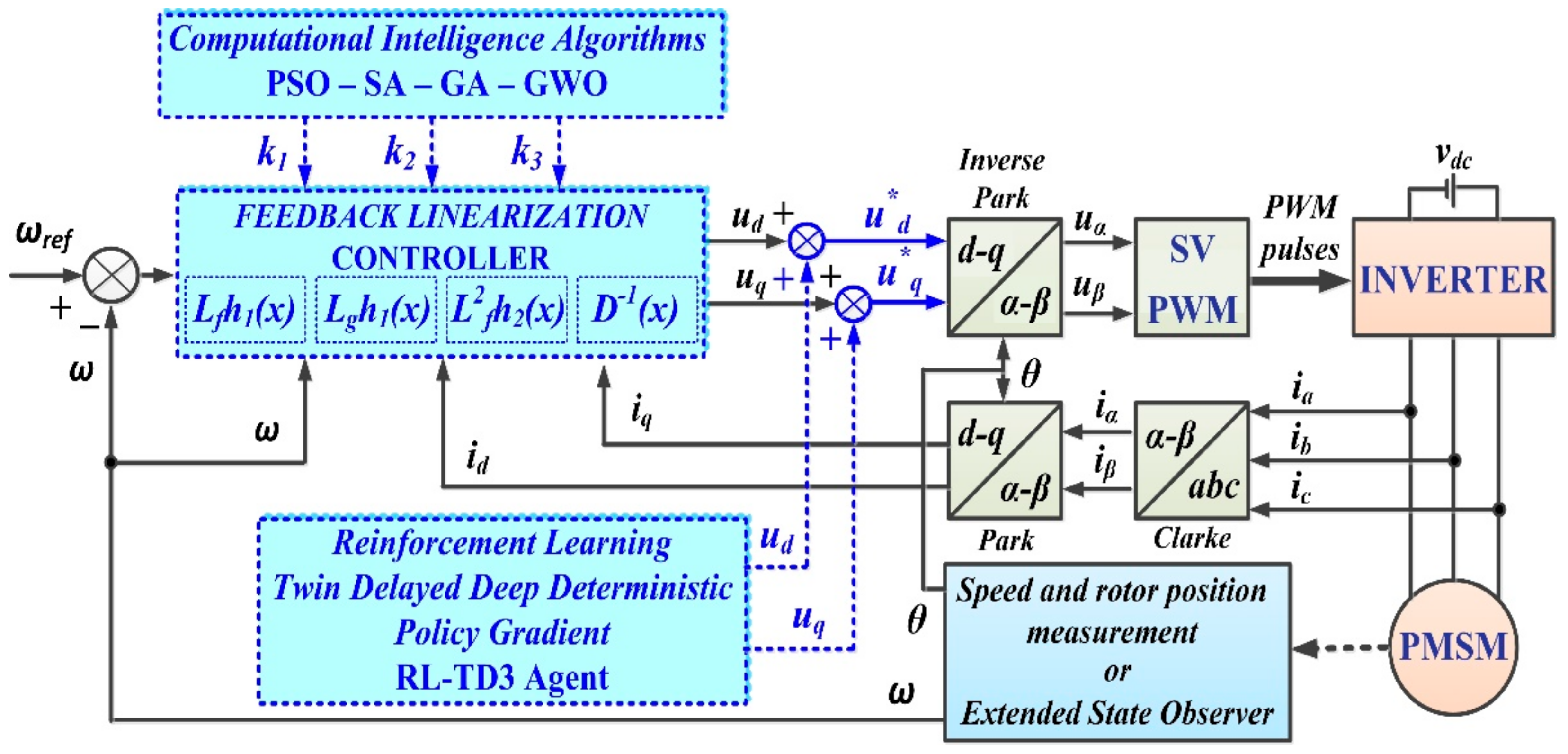
Though the linearization of the model in Section 2 was performed in the classical manner, in this section, the linearization of the nonlinear model (1) of the PMSM will be performed by using the feedback linearization control method. Thus, Figure 3 shows the proposed PMSM–CS–CI control block diagram based on an FL-type controller. The parameters of control laws u_d and u_q will be optimized with CI methods. Furthermore, an optimization of the performance of PMSM–CS–CI will be presented by using an RL-TD3 agent for CCSs.

The system (1) can be rewritten in the form of Equation (9) in order to easily follow the feedback linearization method.

$$\left\{\begin{array}{l}{f}_1=a_{11}{x}_1+a_{12}{x}_2{x}_3\\ f_2=a_{21}{x}_2+a_{22}{x}_1{x}_3+a_{23}{x}_3\\ f_3=a_{31}{T}_L+a_{32}{x}_2+a_{33}{x}_3\end{array}\right.$$

(9)

The notations used in Equation (9) are specified below: $a_{11}=-\frac{R}{L}$, $a_{12}=n_p$, $a_{21}=-\frac{R}{L}$, $a_{22}=-n_p$, $a_{23}=\frac{{\lambda }_0{n}_p}{L}$, $a_{31}=-\frac{1}{J}$, $a_{32}=\frac{3n_p{\lambda }_0}{2J}$, and $a_{33}=-\frac{B}{J}$. Based on these notations, the system (9) becomes:

$$\dot{x}=f(x)+{\displaystyle \sum _{i=1}^m{g}_i(x)u_i};\hspace{1em}i=1,2$$

(10)

In Equation (10), the state vector, the command vector, and the vector functions g_i are defined as follows: $x={[\begin{array}{ccc}{x}_1& x_2& x_3\end{array}]}^T={[\begin{array}{ccc}{i}_d& i_q& \omega \end{array}]}^T$, $u={[\begin{array}{cc}{u}_1& u_2\end{array}]}^T={[\begin{array}{cc}{u}_d& u_q\end{array}]}^T$, $g_1={\left[\begin{array}{ccc}\frac{1}{L}& 0& 0\end{array}\right]}^T$, and $g_2={\left[\begin{array}{ccc}0& \frac{1}{L}& 0\end{array}\right]}^T$.

In the general case, starting from Equation (10), this can be written in the following compact form [17,18,19]:

$$\left\{\begin{array}{l}\dot{x}=f(x)+g(x)u\\ y=h(x)\end{array}\right.$$

(11)

where $x={[x_1,\dots ,x_n]}^T$ denotes the state vector, f(x) and g(x) denote the two n-dimensional smooth vector fields, u denotes the scalar control, y denotes the variable output, and h(x) denotes the scalar function.

Defining the relative order for the output h as a positive integer r results in the following equation:

$$\left\{\begin{array}{l}{L}_g{L}_f^{k}h(x)\equiv 0,\hspace{1em}\forall x\in U, 0\le k\le r-2\\ L_g{L}_f^{k}h(x)\ne 0,\hspace{1em} k=r-1\end{array}\right.$$

(12)

where $L_f^{k}h(x)$ denotes the k-order Lie derivative of h(x) relative to f(x) and $L_g{L}_f^{k}h(x)$ denotes the Lie derivative of $L_f^{k}h(x)$ relative to g(x) [17,18,19].

For linearization, the system output of the following form can be chosen:

$$y=cx$$

(13)

In this sense, the output function is derived until the control u explicitly appears in its expression:

$$y^{(k)}=L_f^{k}h(x)+L_g{L}_f^{k-1}h(x)u,\hspace{1em}k=0,1,\dots ,r$$

(14)

By replacing the relation (12) with (14), the system of equations of the output derivatives can be obtained:

$$\left\{\begin{array}{l}{y}^{(k)}=L_f^{k}h(x),\hspace{1em}k=0,1,\dots ,r-1\\ y^{(r)}=L_f^{r}h(x)+L_g{L}_f^{r-1}h(x)u,\hspace{1em}k=r\end{array}\right.$$

(15)

The following transformation can be defined:

$$z=\left[\begin{array}{l}{z}_1\\ z_2\\ z_3\\ ⋮\\ z_r\\ z_{r+1}\\ ⋮\\ z_n\end{array}\right]=\left[\begin{array}{l}y\\ \dot{y}\\ ⋮\\ y^{r-1}\\ {\eta }_1\\ ⋮\\ {\eta }_{n-r}\end{array}\right]=\left[\begin{array}{l}h(x)\\ L_{f}h(x)\\ ⋮\\ L^{r-1}h(x)\\ {\eta }_1(x)\\ ⋮\\ {\eta }_{n-r}(x)\end{array}\right]=\Phi (x)$$

(16)

In the transformation expressed in relation (16), it can be noted that the new state vector is z, and η is a function that depends on the old state vector x.

Based on these, the nonlinear system (11) to which the transformation (16) is applied can be written in the following form:

$$\left\{\begin{array}{l}\left[\begin{array}{l}{\dot{z}}_1\\ {\dot{z}}_2\\ ⋮\\ {\dot{z}}_{r-1}\\ {\dot{z}}_r\end{array}\right]=\left[\begin{array}{ccccc}0& 1& 0& \cdots & 0\\ 0& 0& 1& \cdots & 0\\ ⋮& ⋮& ⋮& ⋮& ⋮\\ 0& 0& 0& \cdots & 1\\ 0& 0& 0& \cdots & 0\end{array}\right]\left[\begin{array}{l}{z}_1\\ z_2\\ ⋮\\ z_{r-1}\\ z_r\end{array}\right]+\left[\begin{array}{l}0\\ 0\\ ⋮\\ 0\\ 1\end{array}\right]v\\ \left[\begin{array}{l}{\dot{z}}_{r+1}\\ ⋮\\ {\dot{z}}_n\end{array}\right]=\left[\begin{array}{l}{\dot{\eta }}_1(z)\\ ⋮\\ {\dot{\eta }}_{n-r}(z)\end{array}\right]\end{array}\right.$$

(17)

In the system (17), the state vector $z_L={[z_1,\dots ,z_r]}^T$ characterizes the linear subsystem, and the state vector $z_N={[z_{r+1},\dots ,z_n]}^T$ characterizes the nonlinear subsystem. The control law of the nonlinear system is expressed by the following relation: $v=L_f^{k}h[{\Phi }^{-1}(z)]+L_g{L}_f^{r-1}h[{\Phi }^{-1}(z)]u$. The linearized form of this control law can be chosen as follows:

$$v=-k{z}_L=-k_1{z}_1-k_2{z}_2\cdots -k_r{z}_r$$

(18)

where $k_1,\dots ,k_r$ denotes the coefficients of the linearized control law.

By combining Equations (15)–(18), the control law of the nonlinear system (11) can be obtained.

$$u=\frac{-L_f^{r}h[{\Phi }^{-1}(z)]-k{z}_L}{L_g{L}_f^{r-1}h[{\Phi }^{-1}(z)]}$$

(19)

In particular, in the case of the PMSM–CS described by Equation (10), the following relations can be obtained:

$$y=h(x)=\left[\begin{array}{c}{h}_1\\ h_2\end{array}\right]=\left[\begin{array}{c}{x}_1\\ x_3\end{array}\right]=\left[\begin{array}{c}{i}_d\\ \omega \end{array}\right]$$

(20)

where y denotes the output of the system.

As in relation (14), the system output y from relation (20) can be derived, and the following relation can be written:

$${\dot{y}}_1(x)=L_f{h}_1(x)+L_{g_1}{h}_1(x)u_d$$

(21)

in which the following terms can be identified: $L_f{h}_1(x)=f_1(x)$ and $L_g{h}_1(x)=\left[\begin{array}{cc}\frac{1}{L}& 0\end{array}\right]$.

Let us note that the relative degree of the output y₁ is r₁ = 1. Similarly, the output y₂ is derived, and the following relations can be written:

$$\left\{\begin{array}{l}{\dot{y}}_2(x)=L_f{h}_2(x)=f_3(x)\\ {\ddot{y}}_2(x)=L_f^2{h}_2(x)+L_{g_2}{L}_f{h}_2(x)u_q\end{array}\right.$$

(22)

In Equation (22), the sizes $L_f^2{h}_2(x)=a_{32}{f}_2(x)+a_{33}{f}_3(x)$ and $L_{g_2}{L}_f{h}_2(x)=\left[\begin{array}{cc}0& a_{32}/L\end{array}\right]$ are identified. Let us note that the relative degree of output y₁ is r₁ = 1.

By writing the relations (22) in a compact manner, the following relation can be obtained:

$$\left(\begin{array}{c}{\dot{y}}_1(x)\\ {\ddot{y}}_2(x)\end{array}\right)=\left(\begin{array}{c}\frac{d{i}_d}{dt}\\ \frac{d^2\omega }{d^{2}t}\end{array}\right)=A(x)+D(x)\left(\begin{array}{c}{u}_d\\ u_q\end{array}\right)$$

(23)

where $A(x)=\left(\begin{array}{c}{f}_1(x)\\ a_{32}{f}_2(x)+a_{33}{f}_3(x)\end{array}\right)$, and $D(x)=\left(\begin{array}{cc}\frac{1}{L}& 0\\ 0& \frac{a_{32}}{L}\end{array}\right)$ denotes the decoupling matrix.

Thus, the control laws u_d and u_q are obtained in the following form [19]:

$$\left(\begin{array}{c}{u}_d\\ u_q\end{array}\right)=D^{-1}(x)\left[\begin{array}{cc}\left(\begin{array}{c}{v}_1\\ v_2\end{array}\right)& -A(x)\end{array}\right]$$

(24)

where $\det (D)=\frac{1}{L^2}{a}_{32}$ and $D^{-1}=\left(\frac{L^2}{a_{32}}\right)\left(\begin{array}{cc}\frac{a_{32}}{L}& 0\\ 0& \frac{1}{L}\end{array}\right)$.

In Equation (24), ν₁ and ν₂ are components that are included in the new input vector of the system. They are expressed by the following relation:

$$\left(\begin{array}{c}{\nu }_1\\ {\nu }_2\end{array}\right)=\left(\begin{array}{c}{\dot{y}}_1\\ {\ddot{y}}_2\end{array}\right)=\left(\begin{array}{c}{k}_{11}(i_{dref}-i_d)\\ k_{21}({\omega }_{ref}-\omega )+k_{22}({\dot{\omega }}_{ref}-\dot{\omega })\end{array}\right)$$

(25)

By including Equation (25) in (24), the following relation can be obtained:

$$\left(\begin{array}{c}{u}_d\\ u_q\end{array}\right)=\frac{L^2}{a_{32}}\left(\begin{array}{cc}\frac{a_{32}}{L}& 0\\ 0& \frac{1}{L}\end{array}\right)\hspace{0.33em}\left(\begin{array}{c}{k}_{11}(i_{dref}-i_d)-f_1(x)\\ k_{21}({\omega }_{ref}-\omega )+k_{22}({\dot{\omega }}_{ref}-\dot{\omega })-a_{32}{f}_2(x)-a_{33}{f}_3(x)\end{array}\right)$$

(26)

The control laws u_d and u_q can be inferred with components from Equation (26), as in the relations below, and Figure 4 presents the synthesis of the implementation of controls u_d and u_q based on the input variables, states, and parameters of the vector $K=\left[\begin{array}{ccc}{k}_{11}& k_{12}& k_{22}\end{array}\right]$, which will be optimized with CI methods.

$$\left\{\begin{array}{l}{u}_d=L\left(k_{11}{i}_d-f_1(x)\right)\\ u_q=\frac{L}{a_{32}}\left(k_{21}({\omega }_{ref}-\omega )+k_{22}({\dot{\omega }}_{ref}-\dot{\omega })\right.\left.-a_{32}{f}_2(x)-a_{33}{f}_3(x)\right)\end{array}\right.$$

(27)

4. Nonlinear Control for a PMSM

In Section 2 and Section 3, the control laws of the controllers were inferred by simplifying and linearizing the system (1) and describing the PMSM’s operating equations, which were nonlinear. Thus, in this section, the notions and elements of nonlinear systems theory will be used to obtain the control laws u_d and u_q, and the central element, which, from the start, will be a Lyapunov function.

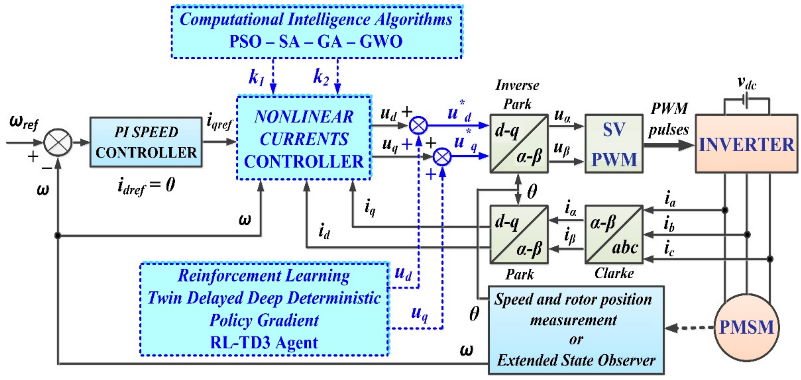
Thus, Figure 5 shows the proposed PMSM–CS–CI control block diagram based on a nonlinear-type controller in which the FOC-type control structure is kept. The parameters of the control laws u_d and u_q will be optimized with CI methods. Moreover, an optimization of the PMSM–CS–CI performance will be presented by using an RL-TD3 agent for the CCS.

Starting from Equation (1) and noting that ${\lambda }_d=\frac{1}{L_d}$ and ${\lambda }_q=\frac{1}{L_q}$, the following form can be obtained [20,26]:

$$\left\{\begin{array}{l}\frac{d{i}_d}{dt}={\lambda }_d{u}_d+f_1\\ \frac{d{i}_q}{dt}={\lambda }_q{u}_q+f_2\end{array}\right.$$

(28)

In Equation (28), the expressions of the terms f₁ and f₂ are given as follows:

$$\left\{\begin{array}{l}{f}_1=-\left(\frac{R_s{i}_d}{L_d}\right)+\left(\frac{L_q{n}_p\omega i_q}{L_d}\right)\\ f_2=-\left(\frac{R_s{i}_q}{L_q}\right)-\left(\frac{L_d{n}_p\omega i_d}{L_q}\right)-\left(\frac{{\lambda }_0{n}_p\omega }{L_q}\right)\end{array}\right.$$

(29)

By choosing a Lyapunov function of the form

$$V=0.5\cdot {\left(i_d-i_{dref}\right)}^2+0.5\cdot {\left(i_q-i_{qref}\right)}^2$$

(30)

and by deriving it, the following form can be obtained:

$$\dot{V}=\left(i_d-i_{dref}\right)\left({\dot{i}}_d-{\dot{i}}_{dref}\right)+\left(i_q-i_{qref}\right)\hspace{0.33em}\left({\dot{i}}_q-{\dot{i}}_{qref}\right)$$

(31)

By using the relations (29), the following equation can be written:

$$\dot{V}=\left(i_d-i_{dref}\right)\left({\lambda }_d{u}_d+f_1-{\dot{i}}_{dref}\right)+\hspace{0.33em}\left(i_q-i_{qref}\right)\left({\lambda }_q{u}_q+f_2-{\dot{i}}_{qref}\right)$$

(32)

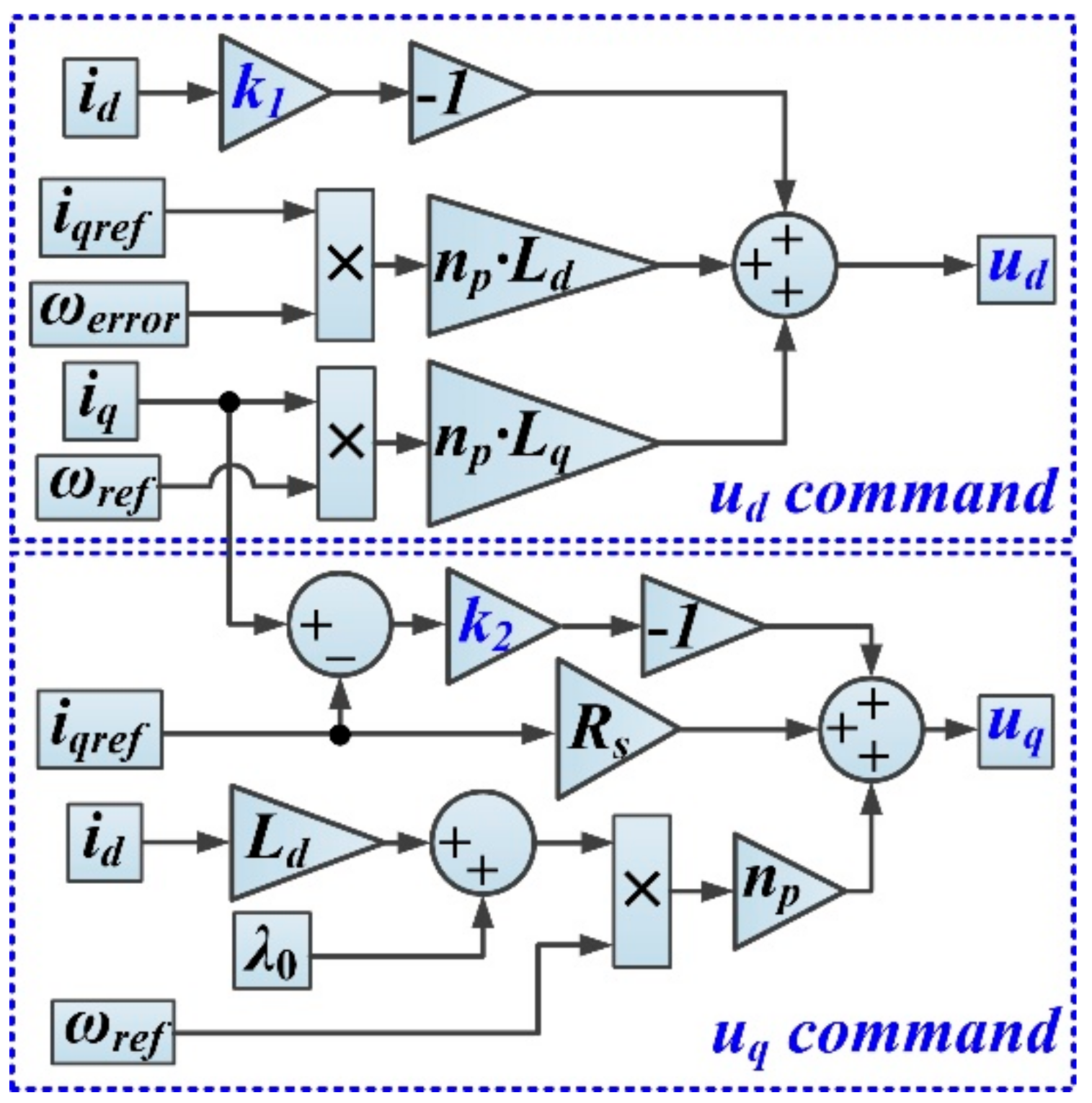
In order to stabilize the system, the control laws u_d and u_q can be chosen from Equation (32) in the following form [20,26]:

$$\left\{\begin{array}{l}{u}_d=\left(\frac{1}{{\lambda }_d}\right)\left(-f_1+{\dot{i}}_{dref}-k_1\left(i_d-i_{dref}\right)\right)\\ u_q=\left(\frac{1}{{\lambda }_q}\right)\left(-f_2+{\dot{i}}_{qref}-k_2\left(i_q-i_{qref}\right)\right)\end{array}\right.$$

(33)

Moreover, by choosing the strictly positive parameters k₁ and k₂, the following equation can be written:

$$\dot{V}=-k_1{\left(i_d-i_{dref}\right)}^2-k_2{\left(i_q-i_{qref}\right)}^2<0$$

(34)

From Equation (34), the asymptotic stability of the closed-loop system can be obtained:

$$\left\{\begin{array}{l}\underset{t\to \infty }{\lim }{i}_d(t)=i_{dref}(t)\\ \underset{t\to \infty }{\lim }{i}_q(t)=i_{qref}(t)\end{array}\right.$$

(35)

If it is assumed that the parametric variations in the expressions of relations f₁ and f₂ given in (29) can be embedded into the form of Equation (36), the robustness of the nonlinear control laws given in Equation (33) can be verified.

$$f_i=f_{in}+\Delta f_i;\hspace{1em}i=1,2$$

(36)

In Equation (36), the nominal values are denoted as f_in, Δf_i represents the variations around the nominal functions, and f_i represents the total actual functions. In addition, it is assumed that parametric uncertainties have the following upper bound:

$$\left|\Delta f_i\right|\le {\beta }_i;\hspace{1em}i=1,\hspace{0.17em}2$$

(37)

By introducing Equation (36) into (28), the following can be written:

$$\left\{\begin{array}{l}\frac{d{i}_d}{dt}={\lambda }_d{u}_d+{\widehat{f}}_1+\Delta f_1\\ \frac{d{i}_q}{dt}={\lambda }_q{u}_q+{\widehat{f}}_2+\Delta f_2\end{array}\right.$$

(38)

In the case of the above disturbed system, the Lyapunov function of the following form can be chosen:

$$V_1=0.5\cdot {\left(i_d-i_{dref}\right)}^2+0.5\cdot {\left(i_q-i_{qref}\right)}^2$$

(39)

Following the technique of Lyapunov functions, as in the previous case, the control laws can be obtained in the following form:

$$\left\{\begin{array}{l}{u}_d=\left(\frac{1}{{\lambda }_d}\right)\left(-{\widehat{f}}_1+{\dot{i}}_{dref}-k_1\left(i_d-i_{dref}\right)-k_{11}sign\left(i_d-i_{dref}\right)\right)\hspace{0.33em}\hspace{0.33em}\hspace{0.33em}\hspace{0.33em}\hspace{0.33em}\\ u_q=\left(\frac{1}{{\lambda }_q}\right)\left(-{\widehat{f}}_2+{\dot{i}}_{qref}-k_2\left(i_q-i_{qref}\right)-k_{22}sign\left(i_q-i_{qref}\right)\right)\end{array}\right.$$

(40)

By choosing $k_{ii}>\beta i,\hspace{0.33em}{k}_i>0$ with i = 1,2, the following equation can be obtained:

$${\dot{V}}_1=\left(i_d-i_{dref}\right)\left(\Delta f_1-k_{11}sign\left(i_d-i_{dref}\right)\right) + \left(i_q-i_{qref}\right)\hspace{0.33em}\left(\Delta f_2-k_{22}sign\left(i_q-i_{qref}\right)\right)+\dot{V}<0$$

(41)

By choosing coefficients k_ii with i = 1,2 in the form

$$\left\{\begin{array}{l}{k}_{11}>{\beta }_1>\left|\Delta f_1\right|\\ k_{22}>{\beta }_2>\left|\Delta f_2\right|\end{array}\right.$$

(42)

the following inequality can be obtained:

$${\dot{V}}_1<\dot{V}<0$$

(43)

From Equation (43), the asymptotic stability of the closed-loop system is inferred, even in the case of parametric disturbance. Figure 6 shows the synthesis of the implementation of controls u_d and u_q based on the input variables, states, and parameters of the vector $K=\left[\begin{array}{cc}{k}_1& k_2\end{array}\right]$, which will be optimized with CI methods.

5. PCH Control for a PMSM

Further to the approach in the previous section regarding the descriptive equations for a nonlinear PMSM, this section focuses on the PCH theory. Thus, it can be started by writing the initial system of Equation (1) in Hamiltonian form and highlighting the energy storage elements, as well as all of the interconnections with the inputs and outputs of the system. The passivity property of the system can be considered, and, by minimizing the total energy function, the control laws u_d and u_q, which drive the closed-circuit system to the proposed steady state, can be obtained [27,28,29].

Thus, Figure 7 shows the control block diagram of the proposed PMSM–CS–CI based on the PCH controller, in which the FOC-type control structure is kept. The parameters of the control laws u_d and u_q will be optimized with CI methods. Moreover, an optimization of the PMSM–CS–CI performance will be presented by using an RL-TD3 agent for the CCS.

By describing the system (1) in the form of a PCH system, as in Equation (44), the algorithm for obtaining the control laws u_d and u_q can be started [27,28,29]:

$$\left\{\begin{array}{l}\dot{x}=\left[J(x)-R(x)\right]\frac{\partial H(x)}{\partial x}+g(x)u\\ y=g^T(x)\frac{\partial H(x)}{\partial x}\end{array}\right.$$

(44)

The notations in Equation (44) are common in descriptions of PCH systems, i.e., $x\in R^n$ denotes the energy variables, $u,y\in R^m$ denotes the input/output port power variables, $R(x)=R^T(x)\ge 0$ denotes the dissipation matrix, g(x) denotes the matrix for the interconnection, $J(x)=J^T(x)$ denotes the skew-symmetric matrix, and H(x) denotes the total stored energy function of the system.

After some calculations and rearrangements of terms, the initial system (1) can be written in the following form:

$$\left\{\begin{array}{l}{L}_d\left(\frac{d{i}_d}{dt}\right)=-R_s{i}_d+L_q{n}_p\omega i_q+u_d\\ L_q\left(\frac{d{i}_q}{dt}\right)=-R_s{i}_q-L_d{n}_p\omega i_d-{\lambda }_0{n}_p\omega +u_q\\ J\left(\frac{d\omega }{dt}\right)=\left(\frac{3n_p}{2}\right)\left[{\lambda }_0{i}_q+\left(L_d-L_q\right)\hspace{0.33em}{i}_d{i}_q\right]-T_L-B_0\omega +f_{\omega }\end{array}\right.$$

(45)

In the system (45), in addition to the usual notations presented in the description of the operating equations of the PMSM, a global term of parametric disturbance and external disturbance can be denoted as f_ω, and it can be expressed as follows:

$$f_{\omega }=-\left[\Delta J\omega -\Delta B\omega +T_L\right.\left.-n_p\left(\Delta L_d-\Delta L_q\right)i_d{i}_q-n_p\Delta {\lambda }_0{i}_q\right]$$

(46)

where $\Delta L_d=L_{dref}-L_d$ denotes the inductance variations on the d-axis, $\Delta L_q=L_{qref}-L_q$ denotes the inductance variations on the q-axis, $\Delta {\lambda }_0={\lambda }_{0ref}-{\lambda }_0$ denotes the flux linkage variations, $\Delta B=B_{ref}-B$ denotes the variations in the viscous friction coefficient, and $\Delta J=J_{ref}-J$ denotes the variations in the moment of inertia of the PMSM’s rotor and load.

In Equation (47), the state, input, and output vectors are defined as is typical in a PCH system.

$$\left\{\begin{array}{l}x={[\begin{array}{ccc}{x}_1& x_2& x_3\end{array}]}^T={[\begin{array}{ccc}{L}_d{i}_d& L_q{i}_q& J\omega \end{array}]}^T\\ u={[\begin{array}{ccc}{u}_d& u_q& f_{\omega }\end{array}]}^T\\ y={[\begin{array}{ccc}{i}_d& i_q& \omega \end{array}]}^T\end{array}\right.$$

(47)

With these elements, the Hamiltonian function can be defined as in the following expression:

$$H(x)=\frac{L_d{i}_d^2}{2}+\frac{L_q{i}_q^2}{2}+\frac{J{\omega }^2}{2}=\frac{x_1^2}{2L_d}+\frac{x_2^2}{2L_q}+\frac{x_3^2}{2J}$$

(48)

By derivation, the following relation can be expressed:

$$\frac{\partial H(x)}{\partial x}={[\begin{array}{ccc}{i}_d& i_q& \omega \end{array}]}^T$$

(49)

The characteristic elements of the PCH system are presented by identifying them in the relations given in the form:

$$J(x)=\left[\begin{array}{ccc}0& 0& n_p{x}_2\\ 0& 0& -n_p(x_1+{\lambda }_0)\\ -n_p{x}_2& n_p(x_1+{\lambda }_0)& 0\end{array}\right];\hspace{0.33em}R(x)=\left[\begin{array}{ccc}{R}_s& 0& 0\\ 0& R_s& 0\\ 0& 0& B\end{array}\right];\hspace{0.33em}g(x)=\left[\begin{array}{ccc}1& 0& 0\\ 0& 1& 0\\ 0& 0& 1\end{array}\right]$$

(50)

The reference vector can be chosen accordingly:

$$x={[\begin{array}{ccc}{x}_{1ref}& x_{2ref}& x_{3ref}\end{array}]}^T=[\begin{array}{ccc}{L}_d{i}_{dref}& L_q{i}_{qref}& J{\omega }_{ref}\end{array}]=[\begin{array}{ccc}0& L_q\left(B\omega -f_{\omega }\right)/\left(n_p{\lambda }_0\right)& J{\omega }_{ref}\end{array}]$$

(51)

The form of the closed-circuit system is shown in the following equation:

$$\dot{x}=\left[J_d(x)-R_d(x)\right]\frac{\partial H(x)}{\partial x}$$

(52)

where J_d(x) denotes the desired interconnection and R_d(x) denotes the desired damping matrix.

Based on these, the relations given in the following equations can be defined:

$$\left\{\begin{array}{l}{J}_d(x)=J(x)+J_a(x)=-J_d^T(x)\\ R_d(x)=R(x)+R_a(x)=R_d^T(x)>0\end{array}\right.$$

(53)

For the closed-circuit system, the Hamiltonian becomes:

$$H_d(x)=\frac{{\left(x_1-x_{1ref}\right)}^2}{2L_d}+\frac{{\left(x_2-x_{2ref}\right)}^2}{2L_q}+\frac{{\left(x_3-x_{3ref}\right)}^2}{2J}$$

(54)

Its derivative can be written in the following form:

$$\partial H_d(x)/\partial x=[\begin{array}{ccc}{i}_d-i_{dref}& i_q-i_{qref}& \omega -{\omega }_{ref}\end{array}]$$

(55)

The matrices J_a and R_a can be chosen in the following form:

$$J_a(x)=\left[\begin{array}{ccc}0& -J_{12}& J_{13}\\ J_{12}& 0& -J_{23}\\ -J_{13}& J_{23}& 0\end{array}\right];\hspace{0.33em}{R}_a(x)=\left[\begin{array}{ccc}{k}_1& 0& 0\\ 0& k_2& 0\\ 0& 0& 0\end{array}\right]$$

(56)

where J₁₂, J₁₃, J₂₃ denote the interconnection parameters and k₁, k₂ denote the damping parameters.

Considering the fact that in the FOC strategy, i_REF is set to zero, the expressions of the control laws u_d and u_q in the first form can be obtained as follows:

$$\left\{\begin{array}{l}{u}_d=-k_1{i}_d-J_{12}\left(i_q-i_{gref}\right)+J_{13}\left(\omega -{\omega }_{ref}\right)-n_p{L}_q{i}_q{\omega }_{ref}\\ u_q=J_{12}{i}_d+R_s{i}_{gref}-k_2\left(i_q-i_{gref}\right)-J_{23}\left(\omega -{\omega }_{ref}\right)+n_p\left(L_d{i}_d+{\lambda }_0\right){\omega }_{ref}\end{array}\right.$$

(57)

Moreover, the global term f_ω becomes:

$$f_{\omega }=-J_{13}{i}_d+J_{23}\left(i_q-i_{gref}\right)-\frac{3}{2}{n}_p\left(L_d{i}_d+{\lambda }_0\right)i_{qref}+B{\omega }_{ref}$$

(58)

Taking the relations (51) into account by reaching the minimum function H_d (x), the desired steady states are reached under the action of the control laws u_d and u_q, by fulfilling the following relations:

$$\left\{\begin{array}{l}{f}_{\omega }=-n_p{\lambda }_0{i}_{qref}\\ J_{13}=-n_p{L}_d{i}_{qref}\\ J_{23}=0\end{array}\right.$$

(59)

By imposing the interconnection parameter J₁₂ = 0, from expressions (57) to (59), the control laws u_d and u_q of the PCH-type controller can be obtained in the form of relations (60):

$$\left\{\begin{array}{l}{u}_d=-k_1{i}_d-n_p{L}_d{i}_{gref}\left(\omega -{\omega }_{ref}\right)-n_p{L}_q{i}_q{\omega }_{ref}\\ u_q=R_s{i}_{qref}-k_2\left(i_q-i_{qref}\right)+n_p\left(L_d{i}_d+{\lambda }_0\right){\omega }_{ref}\end{array}\right.$$

(60)

Figure 8 shows the synthesis of the implementation of the controls u_d and u_q based on the input variables, states, and parameters of the vector $K=\left[\begin{array}{cc}{k}_1& k_2\end{array}\right]$, which will be optimized with CI methods.

6. Computational Intelligence and Reinforcement Learning Algorithms for PMSM Control Optimization

In this section, the synthesis of a series of CI-type algorithms that will be used to optimize the parameters of vector K for each of the four types of controllers described in the previous sections will be presented. In addition, by using the RL-TD3 agent algorithm, improved performance of the PMSM–CS can be obtained by providing CCSs, which will overlap with the command signals provided by the four types of controllers.

In addition, in the case of the LQR-type controller, an RL-TD3 agent algorithm will be used to optimize the LQR-type controller’s parameters due to the structure of the neural network used and the fact that the control can be written as a linear weighted sum of the state variables.

6.1. PSO Algorithm

The proposed error criterion to be minimized for this type of optimization algorithm is presented in the following equation:

$$f(t)={\displaystyle \underset{0}{\overset{t}{\int }}{e}^2(t)dt}$$

(61)

In this equation, the error e(t) denotes the difference between the PMSM’s reference rotor speed and the PMSM’s instantaneous rotor speed:

$$e(t)={\omega }_{ref}(t)-\omega (t)$$

(62)

An analogy can be made between the way that the PSO algorithm works with the representation of the trajectory of a group of particles in the state space, which, after minimizing an error criterion, gives the possibility of realizing its optimal trajectory [30,31,32,33,34]. The position and speed of each particle in the group can be denoted as x_i and v_i. For each of these particles, the personal optimum can be expressed as follows:

$$y_i(t+1)=\left\{\begin{array}{l}{x}_i(t+1)\hspace{0.33em}if\hspace{0.33em}f(x_i(t+1))<f(y_i(t))\\ y_i(t)\hspace{0.33em}else\end{array}\right.$$

(63)

Let us note the neighborhood’s best position with ${\widehat{y}}_i$; the expression for the social optimum for the neighborhood for each particle can be obtained with the following relation:

$$\widehat{y}(t)=\arg \min \left(f(y_1(t)),f(y_2(t)),\dots ,f(y_n(t))\right)$$

(64)

By recurrence, the following relation between the position and the speed of each particle can be obtained:

$$\left\{\begin{array}{c}{v}_{i,j}(t)=w{v}_{i,j}(t)+c_1{r}_{1,j}(t)\left(y_{i,j}(t)-x_{i,j}(t)\right)+c_2{r}_{2,j}(t)\left({\widehat{y}}_{i,j}(t)-{\widehat{x}}_{i,j}(t)\right)\\ x_i(t+1)=x_i(t)+v_i(t+1)\end{array}\right.$$

(65)

In Equation (65), w r denotes the weight of inertia (for example, w = 0.9), $i=1,\dots ,N$, where N denotes the number of particles, $j=1,\dots ,D$, where D denotes the dimension of the problem, r₁ and r₂ are random numbers, and c₁ and c₂ are positive constants. Usually, depending on the complexity of the problem and the capacity of the computing system, the number of particles selected is N = 50, c₁ = 0.12, and c₂ = 1.2.

The execution of this algorithm is stopped either by using a predefined number of iterations or by achieving convergence and providing the solution, which, in our case, represents the parameters of the vector K in the structure of each control law of PMSM–CS–CI.

6.2. SA Algorithm

This optimization algorithm was inspired in its description by the analogy of the states that a solid undergoes during the cooling process. In addition, the system’s energy function can be assimilated into the objective function that is intended to be minimized. By analogy with the process of solid quenching, the minimum function to be optimized is reached when the mobility of molecules is low, namely, at low temperatures. The transition of the states is given with a probability provided by the Boltzmann–Gibbs distribution, which is presented in the following form [30,31,32,33,34]:

$$\varphi \left(x_i(t)\right)=\frac{1}{1+e^{f\left(\frac{x_i(t)}{T(t)}\right)}}$$

(66)

where T(t) denotes the temperature parameter.

The probability of a transition between two points in which x_i and x_j are given takes the following form [30,31,32,33,34]:

$$P_{ij}=\left\{\begin{array}{l}1;\hspace{1em}if\hspace{0.17em}f\left(x_j\right)<f\left(x_i\right)\\ e^{-\frac{f\left(x_j\right)-f\left(x_i\right)}{c_{b}T}};\hspace{1em}otherwise\end{array}\right.$$

(67)

where c_b denotes the Boltzman constant.

At each iteration, the solution can be written in the following form:

$$x(t+1)=x(t)+D(t)r(t)$$

(68)

where D denotes a matrix whose elements contain the maximum change in variables allowed and $r(t)\approx U{(-1,1)}^{n_x}$.

In addition to Equation (68), the law of evolution of the next state can be written as in Equation (69).

$$D(t+1)=(1-\alpha )D(t)+\alpha \omega R(t)$$

(69)

where R(t) denotes a diagonal matrix whose elements are the values of successful changes, and α and ω are constants.

To simulate the decrease in the temperature, the following relation can be used:

$$T(t+1)=\alpha T(t);\hspace{1em}\alpha \in (0, \hspace{0.17em}1)$$

(70)

The algorithm stops when convergence is reached or after a predefined number of iterations.

6.3. GA Algorithm

As indicated by its name, this optimization algorithm is inspired by genetics, i.e., by the way in which a population of chromosomes evolves through various specific mechanisms, such as selection, crossover, mutation, etc. Starting from the objective function that is characteristic of each individual, but also of those in the neighborhood, each chromosome receives a probability of selection for reproduction. This relation can be described by the following expression [30,31,32,33,34]:

$$Adequate(P_{ind})=2-PS+2\left(PS-1\right)\left(P_{ind}-1\right)/N_{ind}$$

(71)

where: P_IND—position of the individual; N_IND—size of the population; PS—selection pressure where $1\le PS\le 2$. It can be noted that the highest value for the fitness function is obtained for P_IND = N_IND, and an unfitness function is obtained for P_IND = 1. Another important step in the genetic algorithm is the selection of parents that will make up the new population from the current population of chromosomes. This can be done in many ways, but the basic idea is to select the best parents in hopes that they will produce the best offspring. In the case of tournament-type selection, each individual in the current population is represented by a space proportional to the value of its assessment function.

In the case of the optimization of the control parameters of PMSM–CS, the algorithm calculates the speed error e_ω and its derivative, as defined in Equations (72) and (73). The output is represented by the variation in the reference current Δi_qref [30,31,32,33,34]:

$$e_{\omega }(k)={\omega }_{ref}-\omega (k)$$

(72)

$$s{e}_{\omega }(k)=e_{\omega }(k)-e_{\omega }(k-1)$$

(73)

where ω_ref denotes the PMSM’s reference rotor speed.

The speed error can be calculated and updated at each step. The numerical representation of each parameter from the K vector of PMSM–CS–CI can be chosen. The crossover probability, defined as p_c, and the mutation probability, defined as p_m, can be chosen. The initial population of parameters K is generated (yielding a random selection result). Δi_qref is generated for each member of the population C_i with $i=1,\dots ,n$. Moreover, the value of the fitness function is assigned to each element of the population C_i, and it is expressed as follows:

$$p_1=e_{\omega }(k)$$

(74)

$$p_2=s{e}_{\omega }(k)$$

(75)

$$F=\frac{1}{{\alpha }_1{p}_1^2+{\alpha }_2{p}_2^2}$$

(76)

The maximum fit of the population C_i becomes C*, and the change in the control action is defined as i_qref*(k) for PMSM–CS–CI:

$$i_{qref}^{\ast }(k+1)=i_{qref}^{\ast }(k)+\Delta i_{qref}^{\ast }(k)$$

(77)

The algorithm stops when convergence is reached or after a predefined number of iterations. The criterion according to which the algorithm is carried out is based on the integral of the timed-weighted absolute error (ITAE) and has the following form:

$$f(t)={\displaystyle \underset{0}{\overset{t}{\int }}t\left|e(t)\right|dt}$$

(78)

6.4. GWO Algorithm

This algorithm is inspired by how the grey wolf hunts in packs to catch prey. Thus, from a hierarchical point of view, the leader and the second most important are denoted as α and β, and the third most important is denoted as δ, while the least important is denoted as ω. By analogy, there are four stages, which are called searching, encircling, attacking, and hunting of the prey. After generating the number of wolves and their initial positions, the first three solutions for the best fitness function can be selected, and they are denoted as α, β, and δ, while another solution is denoted as ω. In addition, at each iteration, the position of the prey X_p(k) and the position of a wolf at the current iteration X(k) can be calculated.

Based on this, the stage called “encircling of the prey” is described by the following equations [30,31,32,33,34]:

$$D=\left|C{X}_p(k)-X(k)\right|$$

(79)

$$X(k+1)=X_p(k)-AD$$

(80)

where k denotes the number of iterations, D denotes the calculation of the vector in order to express the new position of the grey wolf, $A=2a{r}_1-a,\hspace{0.33em}{r}_1\in [0,\hspace{0.17em}1]$ and $C=2a{r}_2,\hspace{0.17em}{r}_2\in [0,\hspace{0.17em}1]$ denote coefficient vectors for program initialization, and a has a linear decrease between 2 and 0.

Noting the position of the wolf at each iteration as (x, y) and the position of the prey as $\left(x\text{'},y\text{'}\right)$, the following equations iteratively define the GWO-type algorithm’s solution [30,31,32,33,34]:

$$\left\{\begin{array}{l}{D}_{\alpha }=\left|C_1{X}_{\alpha }(k)-X(k)\right|\\ D_{\beta }=\left|C_2{X}_{\beta }(k)-X(k)\right|\\ D_{\delta }=\left|C_3{X}_{\delta }(k)-X(k)\right|\end{array}\right.$$

(81)

$$\left\{\begin{array}{l}{X}_1=X_{\alpha }-A_1{D}_{\alpha }\\ X_2=X_{\beta }-A_2{D}_{\beta }\\ X_3=X_{\delta }-A_3{D}_{\delta }\end{array}\right.$$

(82)

$$X(k+1)=\frac{X_1+X_2+X_3}{3}$$

(83)

The algorithm stops after obtaining the minimum of the objective function with an imposed precision or after a predefined number of iterations.

6.5. RL-TD3 Agent Algorithm

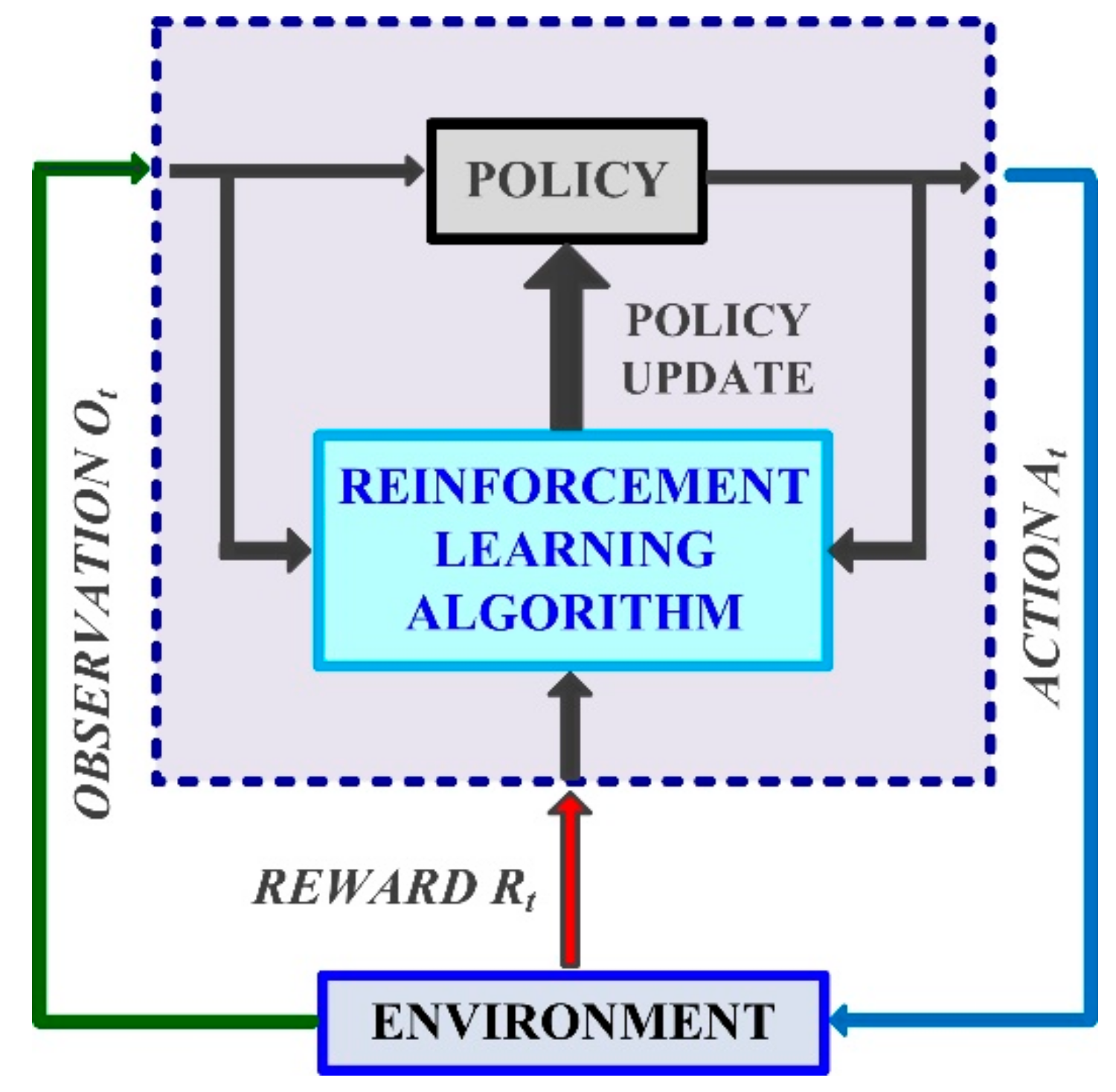
The commonly used machine learning techniques are the following: linear regression, decision tree, support vector machine, neural networks and deep learning, and ensemble of trees. From the point of view of the strategies used in machine learning, the following can be mentioned: unsupervised learning, supervised learning, and RL. Unsupervised learning is typically utilized in the fields of data clustering and dimensionality reduction, while supervised learning mainly deals with classification and regression problems. RL is a framework for learning the relationship between states that are characteristic of the description of a system and the actions on it. The agent achieves the maximization of a reward based on the actions on the system, while also taking observations of the system into account. If it can be considered that the reward can be regarded as an optimization criterion, a very strong analogy with the control of an industrial process can be obtained [35,36,37].

Figure 9 presents the block diagram of the RL-TD3 agent for process control. Finding the optimal policy of the RL-TD3 agent, in this case, can be translated into finding the command signals of the PMSM in order to optimize a performance criterion. Figure 10 shows the implementation of the RL-TD3 controller agent in Matlab/Simulink for the improvement of the performance of PMSM–CS–CI. The analogy with controlling an industrial process can be noted, in the sense that the observations given by currents and speed are the inputs, the outputs represent actions in the form of command signals, and the optimization criterion is in the form of a reward.

The value of the reward is expressed in the following relation:

$$R_C=-\left(5i_{q\_error}^2+5i_{d\_error}^2+5{\omega }_{error}^2+0.1{\displaystyle \sum _j{\left(u_{t-1}^j\right)}^2}\right)$$

(84)

where i_{q_error}, i_{d_error}, and ω_error denote the errors relative to the imposed references of the d-q axis currents i_d and i_q and the rotor speed, respectively. In addition, $u_{t-1}^j$ denotes the weighted actions from the previous step.

The main steps of the RL-TD3 agent can be summarized as follows:

• Formulating the problem;
• Creating the process and reward;
• Training and validating the RL-TD3 agent;
• Deploying the policy.
• The main steps of the training stage are as follows [11,36,37]:
• Selecting the action $A=\mu (S)+N$ for a stochastic noise N and for a current observation S;
• Calculating the action A, reward R, and the next observation S';
• Storing the experience as a 4-tuple $\left(S,A,R,S^{\prime }\right)$;
• M, the experiences $\left(S_i,A_i,R_i,{S^{\prime }}_i\right)$, are randomly generated;
• For each ${S^{\prime }}_i$, which represents a terminal state, the value function target y_i is set to R_i.

Otherwise, the steps below can be followed [11,36,37]:

$$y_i=R_i+\gamma \cdot \min \left({Q^{\prime }}_k\left({S^{\prime }}_k,clip\left({\mu }^{\prime }\left({S^{\prime }}_k\left|{\theta }_{\mu }\right.\right)+\epsilon \right)\hspace{0.33em}\left|{\theta }_{{Q^{\prime }}_k}\right.\right)\right)$$

(85)

The parameters of each critic are expressed in the relation:

$$L_k=\frac{1}{M}{\displaystyle \sum _{i=1}^M{\left(y_i-Q_k\left(S_i,A_i\left|{\theta }_{Qk}\right.\right)\right)}^2}$$

(86)

The parameters of the actor are updated in the following manner:

$${\nabla }_{{\theta }_{\mu }}J=\frac{1}{M}{\displaystyle \sum _{i=1}^M{G}_{ai}{G}_{\mu i}}$$

(87)

where $G_{ai}={\nabla }_A\min \left(Q_k\left(S_i,A\left|{\theta }_Q\right.\right)\right)$, $A=\mu \left(S_i\left|{\theta }_{\mu }\right.\right)$, and $G_{\mu i}={\nabla }_{{\theta }_{\mu }}\mu \left(S_i\left|{\theta }_{\mu }\right.\right)$.

For the following parametric updates, a smoothing factor τ can be chosen, and the following relations can be written:

$${\theta }_{Q{k}^{\prime }}=\tau {\theta }_{Qk}+\left(1-\tau \right){\theta }_{Q{k}^{\prime }}$$

(88)

$${\theta }_{{\mu }^{\prime }}=\tau {\theta }_{\mu }+\left(1-\tau \right){\theta }_{{\mu }^{\prime }}$$

(89)

The characteristic RL-TD3 algorithm stops after obtaining the minimum of the objective function with an imposed precision or after a predefined number of iterations. At this moment, an agent that can be used both for parametric optimization by exploiting the structure of the neural network and for providing CCSs can be created and trained.

7. Numerical Simulations for PMSM–CS–CI

This section presents the results of numerical simulations performed in Matlab/Simulink for the control of a PMSM with the following parameters: stator resistance: R_s = 2.875 Ω, inductances on the d-q axis: L_d = L_q = 0.0085 H, combined inertia of the PMSM rotor and load: J = 8·10⁻³ kg·m², combined viscous friction of the PMSM rotor and load: B = 0.01 N·m·s/rad, flux induced by the permanent magnets of the PMSM rotor in the stator phases: λ = 0.175 Wb, and the pole pair number: n_p = 4.

It can be specified that this motor can be considered a benchmark in Matlab/Simulink simulations because it was presented in a series of articles on control [10,11,15,19,26,29]. The results obtained for PMSM–CS–CI for each of the controllers presented in the previous sections—LQR, FL, nonlinear-type, and PCH controllers—will be comparatively presented, and for each of them, both the initial version of the controller and the versions obtained through the control algorithms’ optimization of parameter K or through the implementation that used the RL-TD3 agent controller with CCSs are presented.

7.1. Numerical Simulations for PMSM–CS–CI Based on the LQR Controller

In order to determine the vector of the command parameters $K=\left[\begin{array}{ccc}{k}_1& k_2& k_3\end{array}\right]$ for the command law (7), the Matlab instruction K = lqr(A,B,Q,R) was used, where Q = diag(40 3000 1) and R = 1 denote the state and control weighting matrices [27].

The transfer function of the PMSM is given in the following equation:

$$H_{PMSM}(s)=\frac{117.6s^2+147.1s}{s^3+339.5s^2+4.366\cdot {10}^{4}s}$$

(90)

The controllability of the system can be verified with a pole at the origin and a complex–conjugate pole pair (−169 ± 121 i), and the parameters of the LQR command law are: k₁ = 14.04, k₂ = 53.31, and k₃ = 1.

By using improved versions of the LQR control law based on the CI algorithms described in Section 6, the following values of the command parameter vector can be obtained: for the PSO-type algorithm, k₁ = 20.78, k₂ = 139.23, and k₃ = 0.17. For the SA-type algorithm, k₁ = 18.42, k₂ = 159.52, and k₃ = 0.2. For the GA-type algorithm, k₁ = 17.35, k₂ = 278.65, and k₃ = 0.29. For the GWO-type , k₁ = 16.16, k₂ = 300, and k₃ = 0.43. Figure 11 presents the evolution of the performance of the PSO-type algorithm for PMSM–CS.

In the case of using the RL-TD3 agent algorithm to optimize the vector of the command parameter K, the reward is used in the form

$$R_O=-\left(40i_q^2+3000{\omega }_{error}^2+{\theta }^2+0.1{\displaystyle \sum _j{\left(u_{t-1}^j\right)}^2}\right)$$

(91)

The state vector in this case is $x={\left[\begin{array}{ccc}{i}_q& \omega & \theta \end{array}\right]}^T$, and the command law can be expressed by the following relation:

$$u=\left[\begin{array}{ccc}{i}_q& {\omega }_{error}& \theta \end{array}\right]\hspace{0.17em}{\left[\begin{array}{ccc}{k}_1& k_2& k_3\end{array}\right]}^T$$

(92)

The RL-TD3 agent used to implement the command law (92) was implemented by using a neural network with one fully connected layer. The vector of parameters K was obtained at the end of the learning period and represented the learnable parameters of the actor.

These could be obtained by using the following functions: actor = getActor (agent) and parameters = getLearnableParameters (actor). The vector obtained were: k₁ = 10, k₂ = 307, and k₃ = 0.3.

In order to improve the performance of PMSM–CS based on the LQR-type controller, an RL-TD3 agent algorithm could be used, which, after the learning phase, was able to provide CCSs that overlapped with the command signals of the LQR-type controller. The implementation of the RL-TD3 agent in Matlab/Simulink is presented in Figure 10, and the reward is given by Equation (84).

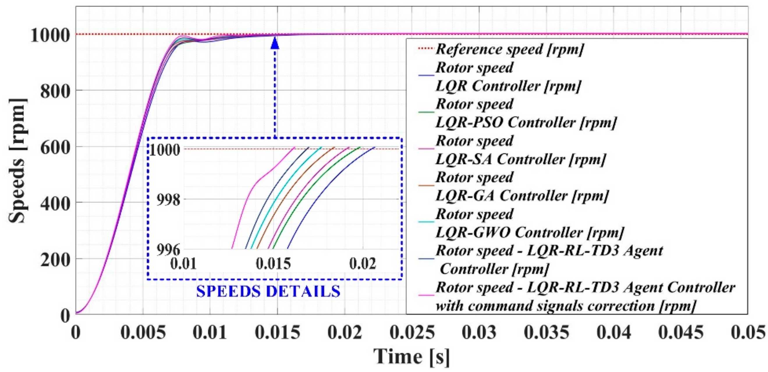
Figure 12 comparatively presents the results of the simulation of the PMSM control in which the control system was made with the LQR-type controller optimized with CI algorithms or based on the RL-TD3 agent controller with CCSs. The evolution of the rotor speed, stator currents, and d-q frame currents for a 1000 rpm step signal and a 0.5 Nm torque load is presented.

Figure 13 comparatively shows the performance of PMSM–CS–CI in terms of speed control for the controllers mentioned above. It improvements in the performance of the basic LQR controller (especially in terms of response time) that used CI algorithms can be noted, and the best results were obtained by using RL-TD3 agent controller with CCSs.

7.2. Numerical Simulations for PMSM–CS–CI Based on the FL Controller

By using improved versions of the FL-type control law based on the CI algorithms described in Section 6, the following values of the command parameter vector could be obtained: PSO-type algorithm: k₁₁ = 97, k₂₁ = 145,294, and k₂₂ = 702; SA-type algorithm: k₁₁ = 101, k₂₁ = 153,785, and k₂₂ = 735; GA-type algorithm: k₁₁ = 104, k₂₁ = 167,119, and k₂₂ = 759; GWO-type algorithm: k₁₁ = 107, k₂₁ = 178,534, and k₂₂ = 767.

Figure 14 presents the evolution of the performance of the SA-type algorithm for PMSM–CS.

In order to improve the performance of PMSM–CS based on the FL-type controller, an RL-TD3 agent algorithm could be used, which, after the learning phase, was able to provide CCSs that overlapped with the command signals of the FL-type controller. The implementation of the RL-TD3 agent in Matlab/Simulink is presented in Figure 10, and the reward is given by Equation (84).

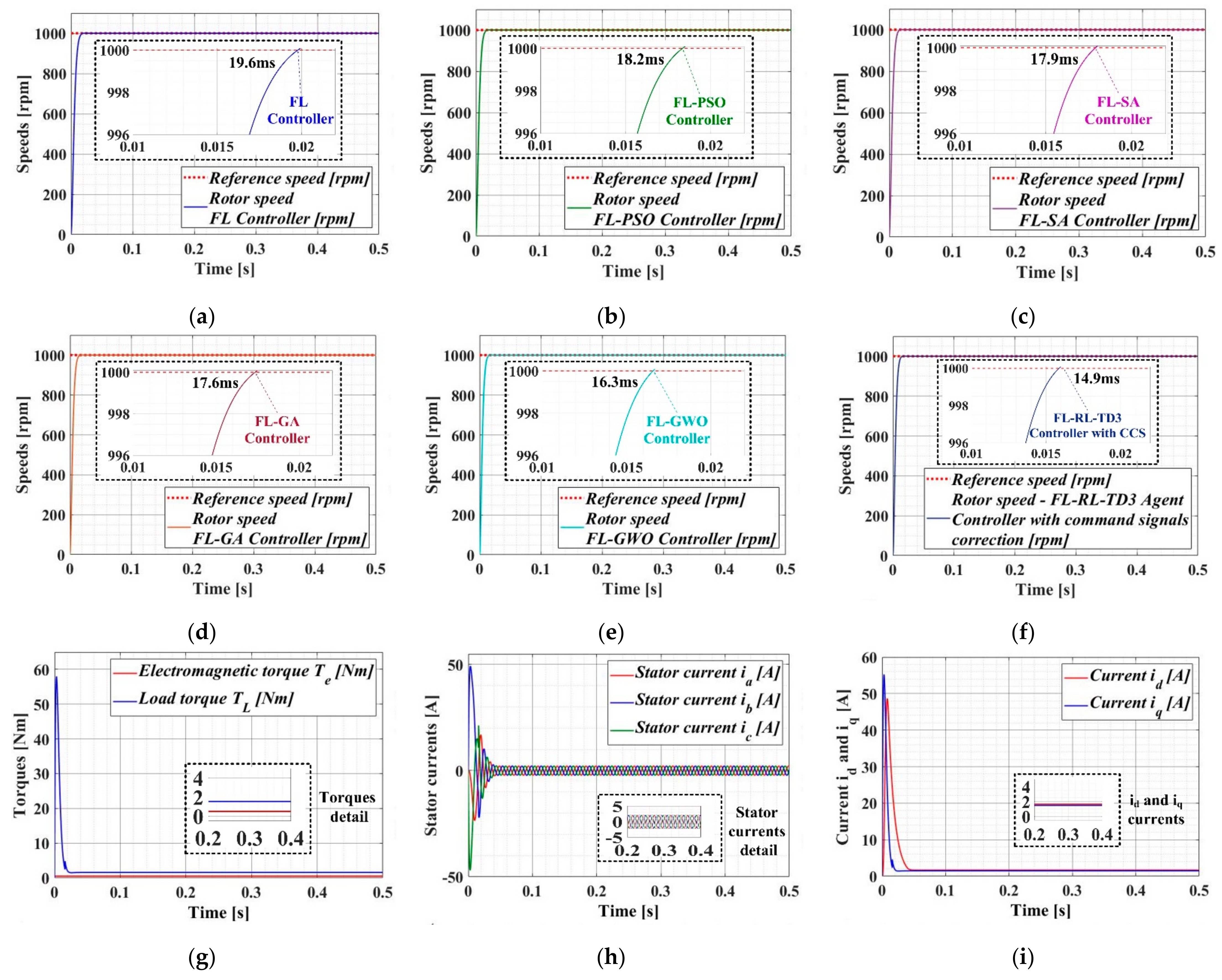
Figure 15 comparatively presents the results of the simulation of the PMSM control in which the control system was made with an FL-type controller that was optimized with CI algorithms or based on the RL-TD3 agent controller with CCSs. The evolution of the rotor speed, load and electromagnetic torques, stator currents, and d-q frame currents for a 1000 rpm step signal and a 0.5 Nm torque load is presented.

Figure 16 comparatively shows the performance of PMSM–CS–CI in terms of speed control for the controllers mentioned above. Improvements in the performance of the basic FL controller (especially in terms of response time) that used the CI algorithms can be noted, and the best results were obtained by using the RL-TD3 agent controller with CCSs.

7.3. Numerical Simulations for PMSM–CS–CI Based on the Nonlinear-Type Controller

By using improved versions of the nonlinear control law based on the CI algorithms described in Section 6, the following values of the command parameter vector could be obtained: PSO-type algorithm: k₁ = 65 and k₂ = 105,200; SA-type algorithm: k₁ = 214 and k₂ = 135,300; GA-type algorithm: k₁ = 529 and k₂ = 172,850; GWO-type algorithm: k₁ = 700 and k₂ = 190,000.

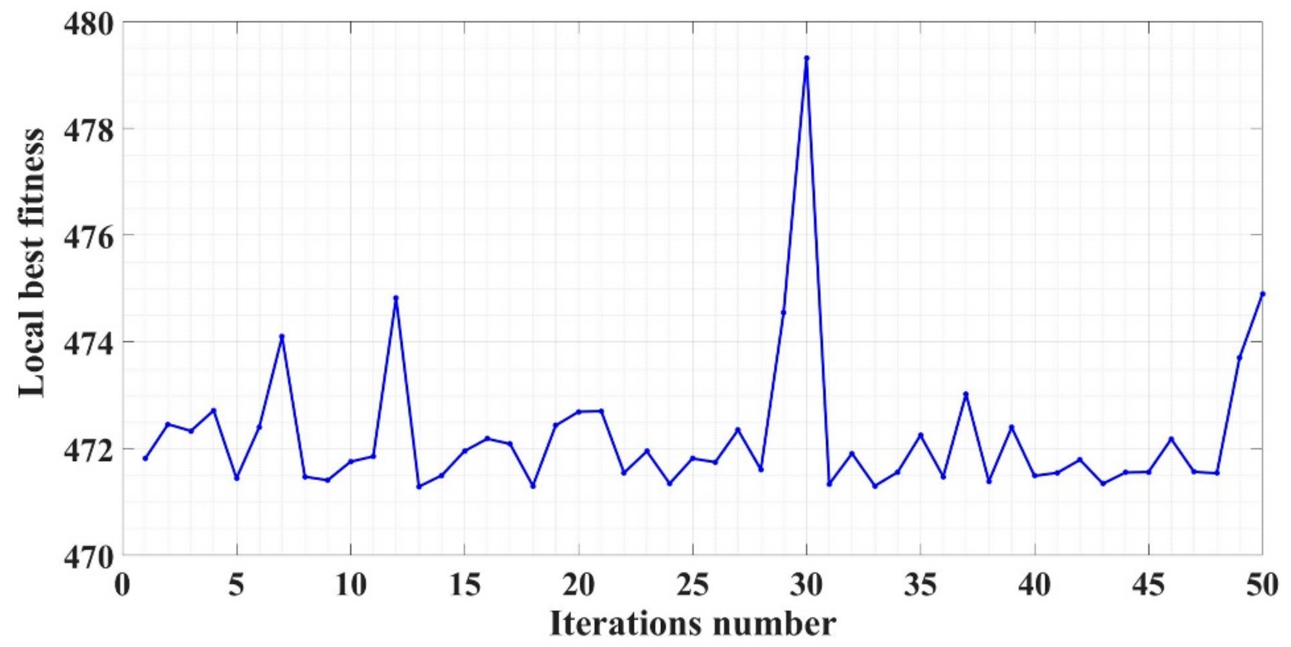
Figure 17 presents the evolution of the performance of the GA-type algorithm for PMSM–CS.

In order to improve the performance of PMSM–CS based on a nonlinear-type controller, an RL-TD3 agent algorithm could be used, which, after the learning phase, was able to provide CCSs that overlapped the command signals of the nonlinear-type controller. The implementation of the RL-TD3 agent in Matlab/Simulink is presented in Figure 10, and the reward is given by Equation (84).

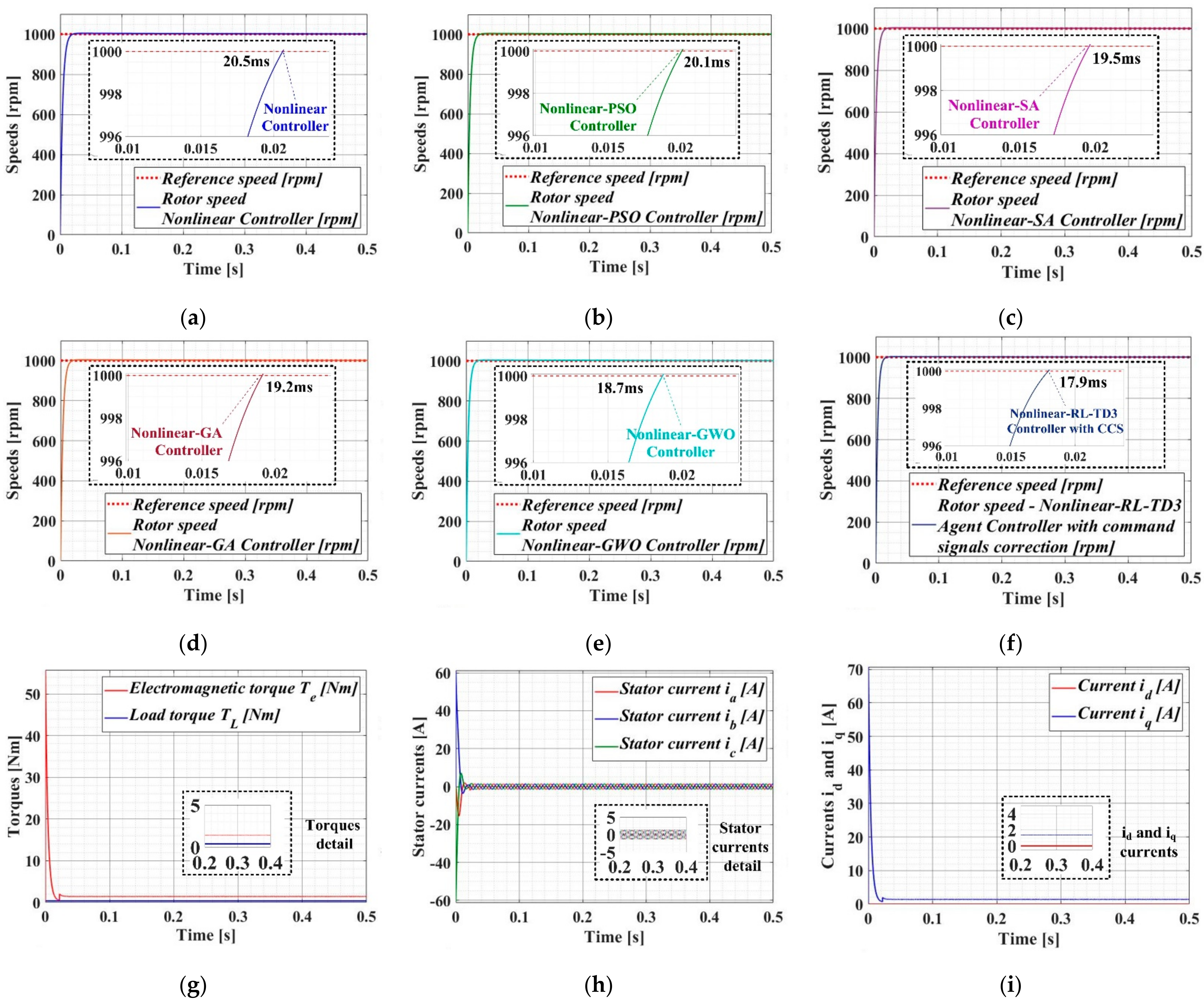
Figure 18 comparatively presents the results of the simulation of the PMSM control in which the control system was made with the nonlinear-type controller optimized with CI algorithms or based on the RL-TD3 agent controller with CCSs. The evolution of the rotor speed, load and electromagnetic torques, stator currents, and d-q frame currents for a 1000 rpm step signal and a 0.5 Nm torque load is presented.

Figure 19 comparatively shows the performance of PMSM–CS–CI in terms of speed control for the controllers mentioned above. Improvements in the performance of the basic nonlinear controller (especially in terms of response time) when using the CI algorithms can be noted, and the best results were obtained by using the RL-TD3 agent controller with CCSs.

7.4. Numerical Simulations for PMSM–CS–CI Based on the PCH Controller

By using improved versions of the PCH-type control law based on the CI algorithms described in Section 6, the following values of the command parameter vector could be obtained: PSO-type algorithm: k₁ = 989 and k₂ = 6.24; SA-type algorithm: k₁ = 921 and k₂ = 5.92; GA-type algorithm: k₁ = 872 and k₂ = 4.98; GWO-type algorithm: k₁ = 825 and k₂ = 4.12.

Figure 20 presents the evolution of the performance of the GA-type algorithm for PMSM–CS.

In order to improve the performance of PMSM–CS based on the PCH-type controller, an RL-TD3 agent algorithm could be used, which, after the learning phase, was able to provide CCSs that overlapped with the command signals of the PCH-type controller. The implementation of the RL-TD3 agent in Matlab/Simulink is presented in Figure 10, and the reward is given by Equation (84). Thus, the evolution of the RL-TD3 agent algorithm’s performance is presented in Figure 21. We specify that the training time of the RL-TD3 agent was of the order of hours.

Figure 22 comparatively presents the results of the simulation of the PMSM control in which the control system was made with the PCH-type controller optimized with CI algorithms or based on the RL-TD3 agent controller with CCSs. The evolution of the rotor speed, load and electromagnetic torques, stator currents, and d-q frame currents for a 1000 rpm step signal and a 0.5 Nm torque load is presented.

Figure 23 comparatively shows the performance of PMSM–CS–CI in terms of speed control for the controllers mentioned above.

Improvements in the performance of the basic PCH-type controller (especially in terms of response time) that used CI algorithms can be noted, and the best results were obtained by using the RL-TD3 agent controller with CCSs.

The parameters used to compare the performance of the PMSM control systems based on the types of controller and the optimization versions described in the previous sections were the response time, overshooting, steady-state error, and speed ripple, which are described in the following relation:

$${\omega }_{rip}=\sqrt{\frac{1}{N}{\displaystyle \sum _{i=1}^N{\left(\omega (i)-{\omega }_{ref}(i)\right)}^2}}$$

(93)

where N denotes the number of samples, ω denotes the rotor speed, and ω_ref denotes the reference rotor speed.

Based on these comparative indicators, the PMSM–CS–CI performance is presented in

Table 1. Performance of the proposed control structures of the PMSM–CS–CI.

Controller		Response Time [ms]	Overshoot [%]	Steady-State Error [%]	Speed Ripple [rpm]
LQR	classic	20.05	0.4	0.2	55.84
	PSO	19.6	0.4	0.2	55.76
	SA	19	0.4	0.2	55.42
	GA	18.2	0.4	0.2	55.13
	GWO	17.5	0.4	0.2	54.90
	RL-TD3	16.8	0.4	0.2	54.59
	RL-TDC with CCS	16	0.4	0.2	54.27
FL	classic	19.6	0.3	0.15	58.11
	PSO	18.2	0.3	0.15	55.99
	SA	17.9	0.3	0.15	55.67
	GA	17.6	0.3	0.15	54.28
	GWO	16.3	0.3	0.15	53.79
	RL-TD3 with CCS	14.9	0.3	0.15	52.31
Nonlinear	classic	20.5	0.2	0.1	43.15
	PSO	20.1	0.2	0.1	43.73
	SA	19.5	0.2	0.1	42.54
	GA	19.2	0.2	0.1	41.96
	GWO	18.7	0.2	0.1	41.40
	RL-TD3 with CCS	17.9	0.2	0.1	38.46
PCH	classic	18.1	0.1	0.05	42.17
	PSO	17.8	0.1	0.05	41.20
	SA	17.2	0.1	0.05	38.17
	GA	16.3	0.1	0.05	37.93
	GWO	15.2	0.1	0.05	37.21
	RL-TD3 with CCS	14.1	0.1	0.05	36.19

.

It can be noted that for each type of controller, the best performance was obtained by using the RL-TD3 agent controller with CCSs in addition to the basic controller.

Thus, for the PMSM–CS presented for the motor that was used as a benchmark in [10,11,15,19,26,29], it can be noted that the best performance was obtained with the PCH-type controller together with an RL-TD3 agent controller with CCSs.

8. Experimental Results

The PMSM used in the numerical simulations as a benchmark and whose characteristics were presented in Section 7 finds its real equivalent in the form of the TelcoMotion DT4260 PMSM. Experiments on this motor controlled by means of the LAUNCHXL-F28379D electronic platform kit with a DRV8305 gate driver were presented by authors of other articles [10,11], so in this article, a PMSM with higher power, the Anaheim Automation EMJ-04APA22, was used, and it was controlled by means of the TMDSHVMTRPFCKIT electronic platform kit.

The main characteristics of the PMSM used were as follows: stator resistance: R_s = 4.7 Ω, inductances on the d-q axis: L_d = L_q = 0.0017 H, combined inertia of the PMSM’s rotor and load: J = 4·10⁻³ kg·m², combined viscous friction of the PMSM’s rotor and load: B = 0.01 N·m·s/rad, flux induced by the permanent magnets of the PMSM’s rotor in the stator phases: λ = 0.175 Wb, and pole pair number: n_p = 4.

TMDSHVMTRPFCKIT is a high-voltage motor control development kit from Texas Instruments that is dedicated to the control of PMSMs. The main MCU of this kit’s board is the TMS320F28069M Real-Time Microcontroller [39,40,41].

The software application that was used to implement the algorithms presented in the previous sections in the hardware described above was developed in the Matlab/Simulink programming environment based on MCB and ECSP for the TI C2000 MCU toolboxes. The usual stages of SIL, PIL, and HIL were completed [40,41]. By using the Matlab/Simulink development environment, the software used in the numerical simulations presented in the previous section could also be used for the real-time implementation. It can be noted that the integral blocks of the type “1/s” were replaced with $k{T}_s/(z-1)$ integral discrete blocks, where T_s denotes the sampling time, k denotes the current step, and s and z are complex continuous and discrete variables, respectively.

The evolution of the PMSM–CS–CI is presented in Figure 24 for a series of reference speed step signals, a load torque of 1 Nm, and an FOC-type control algorithm with a classical PI-type controller. An overshooting of approximately 5% and a steady-state error of less than 1% were noted for both the positive and negative steps of the speed reference of the PMSM rotor.

Figure 25 shows the performance of PMSM–CS–CI for the same series of reference step signals of the PMSM rotor speed and a load torque of 1 Nm, but for the LQR–CI-type PMSM control algorithm. It can be noted that there was a halving of the response time when the overshooting and the steady-state error decreased below 0.4%.

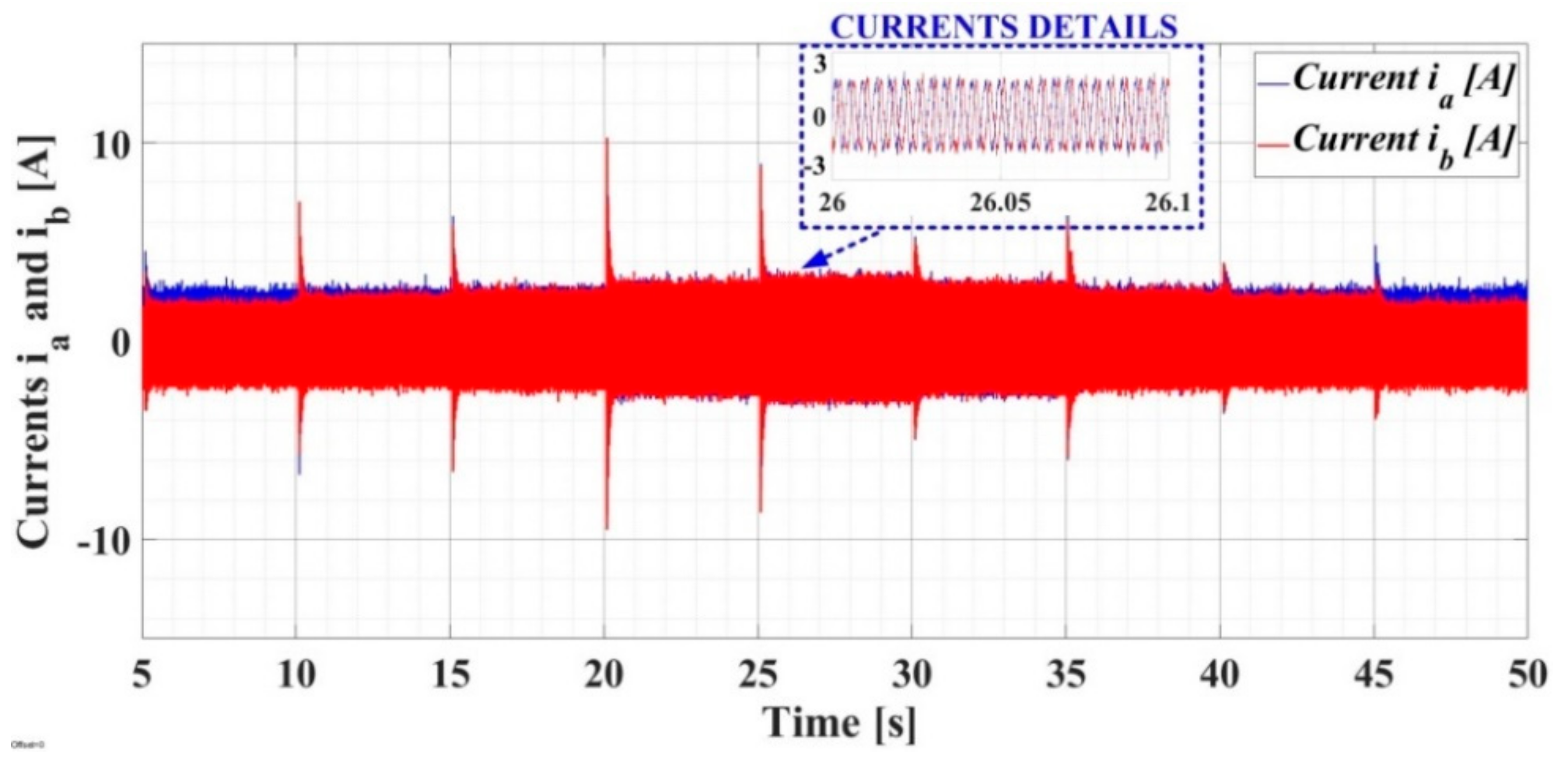
In addition, the real-time evolutions of stator currents i_a and i_b are presented in Figure 26, that of the d-q frame current i_q is presented in Figure 27, and those of the electromagnetic torque T_e and load torque T_L are presented in Figure 28.

It can be specified that the torque load of 1 Nm was provided by the TP 1410 drive system connected to the PMSM shaft. The TP 1410 servo-brake and drive system were programmable and could be used as a load for the PMSM in order to simulate the load torque. The main characteristics of the TP 1410 servo-brake and drive system in terms of the load of the PMSM were a speed ranging between −4000 and 4000 rpm and a maximum braking power of 400 W.

Figure 29 shows the experimental setup which contained the following: TP 1410 servo-brake and drive system, Anaheim Automation EMJ-04APA22 PMSM, PC-host, scope, power source, and TMDSHVMTRPFCKIT development board kit.

9. Conclusions

This article comparatively presents the linear and nonlinear control of a PMSM. The starting elements were the nonlinear operating equations of the PMSM and the global FOC strategy. The LQR algorithm and the algorithm obtained by FL were presented as linear control algorithms. Naturally, the nonlinear approach that used Lyapunov and Hamiltonian functions led to results superior to those of the linear algorithms. By using CI-type algorithms—PSO, SA, GA, and GWO—the performance of PMSM–CS was optimized by obtaining the vectors of the parameters from the control algorithms by optimizing specific performance indices. In addition, superior performance of PMSM–CS was obtained by using RL-type algorithms, which provided CCSs after the training stages. Numerical simulations of a benchmark PMSM were presented for comparison, and the best performance of PMSM–CS was obtained by using a PCH–RL–TD3 agent controller. In addition, an experimental that confirmed the superiority of PMSM–CS–CI was presented. The real-time implementation in embedded systems was achieved by completing the SIL, PIL, and HIL stages of the LQR–CI algorithm (as an example), and the superiority of its performance compared to the use of classical PI-type controllers was proved. In future work, we will deepen the improvements in the performance of linear and nonlinear PMSM controllers by using other CI-type algorithms, as well as other RL-type agent structures.

References

- Liu, D.; Guo, X.; Lei, Y.; Wang, R.; Chen, R.; Chen, F.; Li, Z. An Improved Control Strategy of PMSM Drive System with Integrated Bidirectional DC/DC. Energies 2022, 15, 2214. [Google Scholar] [CrossRef]
- Zhou, K.; Ai, M.; Sun, Y.; Wu, X.; Li, R. PMSM Vector Control Strategy Based on Active Disturbance Rejection Controller. Energies 2019, 12, 3827. [Google Scholar] [CrossRef] [Green Version]
- Lakhe, R.K.; Chaoui, H.; Alzayed, M.; Liu, S. Universal Control of Permanent Magnet Synchronous Motors with Uncertain Dynamics. Actuators 2021, 10, 49. [Google Scholar] [CrossRef]
- Vidlak, M.; Makys, P.; Gorel, L. A Novel Constant Power Factor Loop for Stable V/f Control of PMSM in Comparison against Sensorless FOC with Luenberger-Type Back-EMF Observer Verified by Experiments. Appl. Sci. 2022, 12, 9179. [Google Scholar] [CrossRef]
- Hakami, S.S.; Lee, K.-B. Four-Level Hysteresis-Based DTC for Torque Capability Improvement of IPMSM Fed by Three-Level NPC Inverter. Electronics 2020, 9, 1558. [Google Scholar] [CrossRef]
- Huang, Y.; Zhang, J.; Chen, D.; Qi, J. Model Reference Adaptive Control of Marine Permanent Magnet Propulsion Motor Based on Parameter Identification. Electronics 2022, 11, 1012. [Google Scholar] [CrossRef]
- Liu, F.; Li, H.; Liu, L.; Zou, R.; Liu, K. A Control Method for IPMSM Based on Active Disturbance Rejection Control and Model Predictive Control. Mathematics 2021, 9, 760. [Google Scholar] [CrossRef]
- Zhu, S.; Huang, W.; Zhao, Y.; Lin, X.; Dong, D.; Jiang, W.; Zhao, Y.; Wu, X. Robust Speed Control of Electrical Drives With Reduced Ripple Using Adaptive Switching High-Order Extended State Observer. IEEE Trans. Ind. Electron. 2022, 37, 2009–2020. [Google Scholar] [CrossRef]
- Merabet, A. Cascade Second Order Sliding Mode Control for Permanent Magnet Synchronous Motor Drive. Electronics 2019, 8, 1508. [Google Scholar] [CrossRef] [Green Version]
- Nicola, M.; Nicola, C.-I. Sensorless Fractional Order Control of PMSM Based on Synergetic and Sliding Mode Controllers. Electronics 2020, 9, 1494. [Google Scholar] [CrossRef]
- Nicola, M.; Nicola, C.-I.; Selișteanu, D. Improvement of PMSM Sensorless Control Based on Synergetic and Sliding Mode Controllers Using a Reinforcement Learning Deep Deterministic Policy Gradient Agent. Energies 2022, 15, 2208. [Google Scholar] [CrossRef]
- Xia, C.; Guo, C.; Shi, T. A Neural-Network-Identifier and Fuzzy-Controller-Based Algorithm for Dynamic Decoupling Control of Permanent-Magnet Spherical Motor. In IEEE Transactions on Industrial Electronics; IEEE: Piscataway, NJ, USA, 2010; pp. 2868–2878. [Google Scholar] [CrossRef]
- Valencia-Rivera, G.H.; Merchan-Villalba, L.R.; Tapia-Tinoco, G.; Lozano-Garcia, J.M.; Ibarra-Manzano, M.A.; Avina-Cervantes, J.G. Hybrid LQR-PI Control for Microgrids under Unbalanced Linear and Nonlinear Loads. Mathematics 2020, 8, 1096. [Google Scholar] [CrossRef]
- Xu, W.-J. Permanent Magnet Synchronous Motor with Linear Quadratic Speed Controller. Energy Procedia 2012, 14, 364–369. [Google Scholar] [CrossRef] [Green Version]
- Nicola, M.; Nicola, C.-I. Improved Performance for PMSM Control System Based on LQR Controller and Computational Intelligence. In Proceedings of the International Conference on Electrical, Computer and Energy Technologies (ICECET), Cape Town, South Africa, 9–10 December 2021; pp. 1–6. [Google Scholar] [CrossRef]
- Chen, Y.-T.; Yu, C.-S.; Chen, P.-N. Feedback Linearization Based Robust Control for Linear Permanent Magnet Synchronous Motors. Energies 2020, 13, 5242. [Google Scholar] [CrossRef]
- Li, X.; Chen, X. A Multi-Index Feedback Linearization Control for a Buck-Boost Converter. Energies 2021, 14, 1496. [Google Scholar] [CrossRef]
- Abootorabi Zarchi, H.; Soltani, J.; Arab Markadeh, G. Adaptive Input–Output Feedback-Linearization-Based Torque Control of Synchronous Reluctance Motor without Mechanical Sensor. IEEE Trans. Ind. Electron. 2010, 57, 375–384. [Google Scholar] [CrossRef]
- Nicola, M.; Nicola, C.-I. Improved Performance for PMSM Control System Based on Feedback Linearization and Computational Intelligence. In Proceedings of the International Conference on Electrical, Computer and Energy Technologies (ICECET), Cape Town, South Africa, 9–10 December 2021; pp. 1–6. [Google Scholar] [CrossRef]
- Fezzani, A.; Drid, S.; Makouf, A.; Chrifi-alaoui, L.; Ouriagli, M.; Delahoche, L. Robust control of permanent magnet synchronous motor. In Proceedings of the 15th International Conference on Sciences and Techniques of Automatic Control and Computer Engineering (STA), Hammamet, Tunisia, 21–23 December 2014; pp. 711–718. [Google Scholar] [CrossRef]
- Fezzani, A.; Drid, S.; Makouf, A.; Chrifi-Alaoui, L.; Ouriagli, M. Speed Sensoless Robust Control of Permanent Magnet Synchronous Motor Based on Second-Order Sliding-Mode Observer. Serb. J. Electr. Eng. 2014, 11, 419–433. [Google Scholar] [CrossRef] [Green Version]
- Jeong, Y.W.; Choo Chung, C. Nonlinear Current Control with Modified Torque Modulation for Permanent Magnet Synchronous Motors. In Proceedings of the 59th IEEE Conference on Decision and Control (CDC), Jeju, Republic of Korea, 14–18 December 2020; pp. 928–933. [Google Scholar] [CrossRef]
- Dini, P.; Saponara, S. Cogging Torque Reduction in Brushless Motors by a Nonlinear Control Technique. Energies 2019, 12, 2224. [Google Scholar] [CrossRef] [Green Version]
- Lee, I.; Kim, Y.; Shin, D.; Lee, Y.; Chung, C.C. Nonlinear adaptive speed control for permanent magnet synchronous motors under unbalanced resistances. In Proceedings of the IECON 2015—41st Annual Conference of the IEEE Industrial Electronics Society, Yokohama, Japan, 9–12 November 2015; pp. 1692–1697. [Google Scholar] [CrossRef]
- Abdul-Adheem, W.R.; Ibraheem, I.K. Improved Sliding Mode Nonlinear Extended State Observer based Active Disturbance Rejection Control for Uncertain Systems with Unknown Total Disturbance. Int. J. Adv. Comput. Sci. Appl. 2016, 7, 80–93. [Google Scholar] [CrossRef] [Green Version]
- Nicola, M.; Nicola, C.-I. Improved Performance of PMSM Control Based on Nonlinear Control Law and Computational Intelligence. In Proceedings of the International Conference on Electrical, Computer and Energy Technologies (ICECET), Prague, Czech Republic, 20–22 July 2022; pp. 1–8. [Google Scholar] [CrossRef]
- Liu, X.; Yu, H.; Yu, J.; Zhao, Y. A Novel Speed Control Method Based on Port-Controlled Hamiltonian and Disturbance Observer for PMSM Drives. IEEE Access 2019, 7, 111115–111123. [Google Scholar] [CrossRef]
- Zhao, Y.; Yu, H.; Wang, S. Development of Optimized Cooperative Control Based on Feedback Linearization and Error Port-Controlled Hamiltonian for Permanent Magnet Synchronous Motor. IEEE Access 2021, 9, 141036–141047. [Google Scholar] [CrossRef]
- Nicola, M.; Nicola, C.-I. Improved Performance for the PMSM Control Based on PCH Controller and Computational Intelligence. In Proceedings of the 19th IEEE International Multi-Conference on Systems, Signals & Devices (SSD), Setif, Algeria, 6–10 May 2022; pp. 1650–1657. [Google Scholar] [CrossRef]
- Demir, G.; Vural, R.A. Speed Control Method Using Genetic Algorithm for Permanent Magnet Synchronous Motors. In Proceedings of the 6th International Conference on Control Engineering & Information Technology (CEIT), Istanbul, Turkey, 25–27 October 2018; pp. 1–6. [Google Scholar] [CrossRef]
- Wang, C.-S.; Guo, C.-W.C.; Tsay, D.-M.; Perng, J.-W. PMSM Speed Control Based on Particle Swarm Optimization and Deep Deterministic Policy Gradient under Load Disturbance. Machines 2021, 9, 343. [Google Scholar] [CrossRef]
- Mohan, P.V.; Dixit, S.; Gyaneshwar, A.; Chadha, U.; Srinivasan, K.; Seo, J.T. Leveraging Computational Intelligence Techniques for Defensive Deception: A Review, Recent Advances, Open Problems and Future Directions. Sensors 2022, 22, 2194. [Google Scholar] [CrossRef] [PubMed]
- Rao, H.; Jia, H.; Wu, D.; Wen, C.; Li, S.; Liu, Q.; Abualigah, L. A Modified Group Teaching Optimization Algorithm for Solving Constrained Engineering Optimization Problems. Mathematics 2022, 10, 3765. [Google Scholar] [CrossRef]
- Rahman, M.A.; Sokkalingam, R.; Othman, M.; Biswas, K.; Abdullah, L.; Abdul Kadir, E. Nature-Inspired Metaheuristic Techniques for Combinatorial Optimization Problems: Overview and Recent Advances. Mathematics 2021, 9, 2633. [Google Scholar] [CrossRef]
- Song, Z.; Yang, J.; Mei, X.; Tao, T.; Xu, M. Deep reinforcement learning for permanent magnet synchronous motor speed control systems. Neural Comput. Appl. 2021, 33, 5409–5418. [Google Scholar] [CrossRef]
- Faria, R.d.R.; Capron, B.D.O.; Secchi, A.R.; de Souza, M.B., Jr. Where Reinforcement Learning Meets Process Control: Review and Guidelines. Processes 2022, 10, 2311. [Google Scholar] [CrossRef]
- MathWorks—Reinforcement Learning Toolbox™ User’s Guide. Available online: https://www.mathworks.com/help/reinforcement-learning/getting-started-with-reinforcement-learning-toolbox.html?s_tid=CRUX_lftnav (accessed on 2 December 2021).
- MathWorks—Twin-Delayed Deep Deterministic Policy Gradient Reinforcement Learning Agent. Available online: https://www.mathworks.com/help/reinforcement-learning/ug/td3-agents.html (accessed on 15 December 2021).
- MathWorks—Motor Control Blockset Documentation. Available online: https://www.mathworks.com/help/mcb/index.html (accessed on 7 February 2022).
- MathWorks—Embedded Coder Support Package for Texas Instruments C2000 Processors. Available online: https://www.mathworks.com/help/supportpkg/texasinstrumentsc2000/index.html (accessed on 14 February 2022).
- MathWorks—Run Real-Time Simulation of Permanent Magnet Synchronous Motor. Available online: https://www.mathworks.com/help/slrealtime/ug/apply-slrt-to-simulate-pms-motor-example.html (accessed on 21 February 2022).
- Koulamas, C.; Lazarescu, M.T. Real-Time Embedded Systems: Present and Future. Electronics 2018, 7, 205. [Google Scholar] [CrossRef]
Figure 1.
The proposed control block diagram of the PMSM–CS–CI based on an LQR-type controller.
Figure 2.
Schematic representation of the LQR controller: ud and uq commands.
Figure 3.
The proposed control block diagram of PMSM–CS–CI based on an FL-type controller.
Figure 4.
Schematic representation FL controller: ud and uq commands.
Figure 5.
The proposed PMSM–CS–CI control block diagram based on a nonlinear-type controller.
Figure 6.
Schematic representation of a nonlinear-type controller: ud and uq commands.
Figure 7.
Figure 8.
Schematic representation of a PCH controller: ud and uq commands.
Figure 9.
Block diagram of the RL for process control.
Figure 10.
Matlab/Simulink implementation of the RL-TD3 agent for the proposed controllers.
Figure 11.
Evolution of the performance of the PSO-type algorithm.
Figure 12.
Time evolution parameters of the PMSM–CS–CI based on the LQR-type controller: (a) rotor speed—LQR; (b) speed—LQR–PSO; (c) speed—LQR–SA; (d) speed—LQR–GA; (e) speed—LQR–GWO; (f) speed—LQR–RL–TD3; (g) speed—LQR–RL–TD3 with CCSs; (h) stator currents ia, ib, and ic; (i) currents id and iq.
Figure 13.
Comparison of the time evolution of speed for PMSM–CS–CI based on the LQR-type controller.
Figure 14.
Evolution of the performance of the SA-type algorithm.
Figure 15.
Time evolution of the parameters of the PMSM–CS–CI based on the FL-type controller: (a) rotor speed—FL; (b) speed—FL–PSO; (c) speed—FL–SA; (d) speed—FL–GA; (e) speed—FL–GWO; (f) speed—FL–RL–TD3 with CCSs; (g) electromagnetic and load torques; (h) stator currents ia, ib, and ic; (i) currents id and iq.
Figure 16.
Comparison of the time evolution of speed for PMSM–CS–CI based on the FL-type controller.
Figure 17.
Evolution of the performance of the GA-type algorithm.
Figure 18.
Time evolution parameters of the PMSM–CS–CI based on the nonlinear-type controller: (a) rotor speed—nonlinear; (b) speed—nonlinear–PSO; (c) speed—nonlinear–SA; (d) speed—nonlinear–GA; (e) speed—nonlinear–GWO; (f) speed—nonlinear–RL–TD3 with CCSs; (g) electromagnetic and load torques; (h) stator currents ia, ib, and ic; (i) currents id and iq.
Figure 19.
Comparison of the time evolution of speed for PMSM–CS–CI based on the nonlinear-type controller.
Figure 20.
Evolution of the performance of the GWO-type algorithm.
Figure 21.
Evolution of the reward for the RL-TD3 agent algorithm’s performance.
Figure 22.
Time evolution parameters of the PMSM–CS–CI based on the PCH-type controller: (a) rotor speed—PCH; (b) speed—PCH–PSO; (c) speed—PCH–SA; (d) speed—PCH–GA; (e) speed—PCH–GWO; (f) speed—PCH–RL–TD3 with CCSs; (g) electromagnetic and load torques; (h) stator currents ia, ib, and ic; (i) currents id and iq.
Figure 23.
Comparison of the time evolution of speed for PMSM–CS–CI based on the PCH-type controller.
Figure 24.
Real-time speed evolution of PMSM–CS–CI based on the PI-type controller.
Figure 25.
Real-time speed evolution of PMSM–CS–CI based on the LQR-type controller.
Figure 26.
Real-time evolution of currents ia and ib for PMSM–CS–CI based on the LQR-type controller.
Figure 27.
Real-time evolution of current iq for PMSM–CS–CI based on the LQR-type controller.
Figure 28.
Real-time evolution of torques Te and TL for PMSM–CS–CI based on the LQR-type controller.
Figure 29.
Experimental setup for testing the PMSM–CS–CI.