
Local Linear Approximation Algorithm for Neural Network

1
Department of Statistics, Pennsylvania State University, University Park, PA 16802, USA
2
Corporate Model Risk, Wells Fargo Bank, Charlotte, NC 28202, USA
*
Author to whom correspondence should be addressed.
†
These authors contributed equally to this work.
Mathematics 2022, 10(3), 494; https://0-doi-org.brum.beds.ac.uk/10.3390/math10030494
Submission received: 14 December 2021
/
Revised: 23 January 2022
/
Accepted: 28 January 2022
/
Published: 3 February 2022
(This article belongs to the Special Issue Statistical Methods in Data Mining)
Abstract
:This paper aims to develop a new training strategy to improve efficiency in estimation of weights and biases in a feedforward neural network (FNN). We propose a local linear approximation (LLA) algorithm, which approximates ReLU with a linear function at the neuron level and estimate the weights and biases of one-hidden-layer neural network iteratively. We further propose the layer-wise optimized adaptive neural network (LOAN), in which we use the LLA to estimate the weights and biases in the LOAN layer by layer adaptively. We compare the performance of the LLA with the commonly-used procedures in machine learning based on seven benchmark data sets. The numerical comparison implies that the proposed algorithm may outperform the existing procedures in terms of both training time and prediction accuracy.
1. Introduction
Despite that neural networks have many successful applications, there is a long-standing challenge of training feedforward neural network (FNN) models efficiently to strike a balance between training time and prediction performance. Stochastic gradient descent [1,2,3] is widely used for training neural networks, but it has a slow learning rate and noisy training curves in the beginning of the training epochs.
In order to reduce total training iterations and consequently training time, while achieving high generalization ability, many studies have developed different efficient training algorithms for neural networks, among which linear approximation of the neural network received lots of attentions. Douglas and Meng [4], Singhal and Wu [5] and Stan and Kamen [6] developed linearized least squares using Kalman recursion to update weight parameters. They demonstrated increased training efficiency of this technique compared to gradient descent. However, these methods lacked robustness in terms of model accuracy. Kollias and Anastassiou [7] developed an adaptive least squares algorithm based on the Marquardt-Levenberg optimization algorithm. See Ngia and Sjoberg [8], Kim and Lee [9] and Zhou and Si [10] for other Marquardt-Levenberg based methods. Moreover, Maddox et al. [11], Khan et al. [12] and Mu et al. [13] suggested linearizing neural network with first order Taylor expansion followed by Gaussian process for inference. However, these methods only worked on pre-trained networks but not random initialization [14].
The work in this paper aims to address the problem from a different point of view, and develop a reliable training algorithm called Local Linear Approximation (LLA) Algorithm. In each iteration, LLA uses the first order Taylor expansion to locally approximate activation functions of each neuron. It computes estimated gradient and Hessian matrix, and updates weights and biases in the spirit of Fisher scoring algorithm. Algorithms taking into account Fisher information or Hessian matrix have been proposed via natural gradient descent [15,16]. However, the proposed LLA is different from the existing algorithms. See Section 2.1 for more details. We develop LLA for both regression and classification problems. The high-level summary of the major contributions of this work are shown below:
(a) We derive a novel adaptive method, LLA, which leverages the ideas of linearizing neural network and iterative Fisher scoring, aiming at reducing training time while achieving higher prediction performance than current baselines. Distinguished from existing methods that linearize neural networks, LLA has a unique initialization procedure.
(b) We investigate the convergence behavior of LLA by establishing a connection between the Fisher scoring algorithm and the iterative regression. The connection implies that LLA and Fisher scoring algorithms share the same rate of convergence. Thus, the LLA has a quadratic convergence rate.
(c) As an extension of the one-hidden-layer LLA, we built a layer-wise optimized adaptive neural network (LOAN) for further improvement. The performance of LLA with multiple hidden layers is examined. The experiments demonstrate that shallow LOAN achieves both stable performance and high prediction accuracy level.
(d) We use several benchmark data sets to illustrate and evaluate our proposed method. The results indicate that LLA has a faster convergence rate and outperforms existing optimization methods and machine learning models in terms of prediction on both training and testing data.
2. New Method for Constructing Neural Network
According to the universal approximation theorem [17,18], provided that the network has enough hidden units, an FNN with one-hidden-layer and a linear output layer may approximate any Borel measurable functions well (Section 6.4.1 in [19]). It is common to consider a deep neural network for better prediction performance, but in practice one-hidden-layer neural network with a large number of nodes can still achieve high prediction performance [20,21], which is an easy starting point to explain our proposed LLA method.
2.1. Regression Settings
Consider an one-hidden-layer neural network with nodes:
where is the p-dimensional input vector, W and are the weight matrix and the bias vector in the first hidden layer, respectively, is the j-th row of W corresponding to the jth node, and is the j-th element of . Throughout this paper, we set , the ReLU activation function. Consider a linear regression model in the output layer
For this neural network, the parameters to be optimized are W, a weight matrix, , a -dimensional vector, , a dimensional vector and , a one-dimensional parameter. Denote , and . Let . Suppose that we have a set of sample , . In the literature, the estimation of is to minimize the least squares (LS) function
which is highly nonlinear in . Hence, parameter estimation is challenging for deep neural network.
To tackle these problems, we propose an algorithm to minimize (3). Given in the current step, we propose to approximate by a linear function based on the first-order Taylor expansion of :
We refer (4) to as local linear approximation (LLA) since it is linear approximation with first order Taylor expansion at the neuron level. For any function f, let be an approximation of f by (4) throughout the paper. Thus, is approximated by:
where and . For , define
and
Further define
and
which is a -dimensional vector. With the aid of approximation (5), the objective function in (3) is approximated by
which is a least squares function of linear regression with the response and predictors .
Theorem 1.
Let be the value of at the c-th step. Then
The proof of Theorem 1 is given in Appendix A.1 of this paper. Theorem 1 implies that updating based on (the second equation) is actually equivalent to updating based on (the first equation). Let
where . Thus is a linear function of while it is nonlinear in . This enables us to update easily.
Denote the resulting least squares estimates of , and by , and , respectively. By the definition of and , we can update and as follows
for . If is very close to zero, one may simply set and . The LLA algorithm is to firstly update by least squares estimates of Equation (10). Then, the estimates of W and are obtained by Equation (13). The estimation process is conducted iteratively till convergence. The procedure can be summarized in Algorithm 1.
Motivated by single index models, we design an initialization procedure for W and with nodes as follows. Firstly, we fit data with a linear regression model and obtain the least squares estimates for the coefficients of , denoted by , and the intercept, denoted by . Let , be quantile points of , . We set initial value:
for . Since the objective function is nonconvex, numerical minimization algorithm may depend on the initial value. We find that the proposed initialization strategy works reasonably well in practice. We have conducted some numerical comparison between this initialization procedure and the Xavier initialization strategy, which is based on randomization. Based on our simulation study, the proposed initialization procedure has a better and more stable performance than the Xavier initialization strategy.
| Algorithm 1 Local Linear Approximation (LLA) Algorithm for Regression |
Input: Given data and the number of nodes Initialization: Get initial values for and in Equation (14) Output: W and
|
To understand the convergence behavior of the proposed LLA algorithm, let us briefly describe the Fisher scoring algorithm for a general nonlinear least squares problem. Let
where is a general nonlinear function with existing finite second-order derivatives with respect to , a general parameter vector. Denote and to be the gradient and Hessian matrix of , respectively. The Fisher scoring algorithm is to update by
where stands for an estimate of .
Similar to the proof of Theorem 1, we can rewrite into the following form
which is the solution of the least squares problem
given .
Theorem 2.
For given , let . Then (10) coincides with
The proof of Theorem 2 is given in Appendix A.2 of this paper.
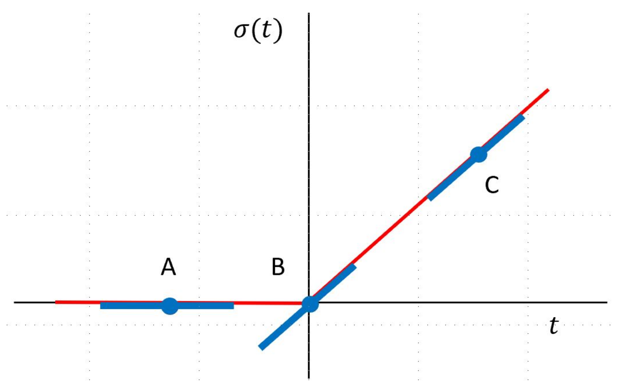
Based on Theorem 2, we may show that the proposed LLA algorithm shares the same convergence rate of the Fisher scoring algorithm. Thus, the convergence rate of the proposed LLA algorithm is quadratic. The Fisher scoring algorithm has been proposed for FNN back in 1990s [22]. Recently, researchers use Fisher information or Hessian matrix information by constructing natural gradient descent [15,16,23]. A natural question which arises here is why the Fisher scoring algorithm is not implemented directly. We have compared the LLA algorithm and the Fisher scoring algorithm via numerical simulation. Our numerical comparison implies that the LLA algorithm is more stable and converges faster than the Fisher scoring algorithm. This may be because is linear in , and (10) provides a better approximation than (15) for both and . In addition, the form of ReLU activation function implies that its first-order derivative is bounded, and its second-order derivative is 0 if it exists. The LLA algorithm takes advantages of it since the LLA in (4) is based on , the first-order Taylor expansion of . Figure 1 presents an illustration of the LLA of ReLU activation function at three different locations.
2.2. Classification
2.2.1. Binary Classification
For a classification problem, the output layer is
where . Thus, training an FNN reduces to estimating by maximizing the log-likelihood function
where . We approximate in the same way as in (4) and approximate similarly by:
where is defined in Equation (5). Let and be the gradient and Hessian matrix of , respectively.
According to Theorems 1 and 2 for regression in Section 2.1, extension to classification involves no fundamentally new ideas. Thus, let be the value of at the c-th step, can be updated based on
and the convergence rate is quadratic as well.
This implies that we can iteratively update using , in which is defined similarly as in (12) and is a linear function of . Thus, we can directly apply logistic regression of on and obtain an estimate of . To save computational cost, we use one-step iteration rather than a full iteration in the logistic regression. The initial values play an important role in the model performance since the log-likelihood function is nonconcave. Similarly, we propose a method to construct initial values of W and for classification. We fit data using a logistic regression model and obtain the estimates of the intercept and the coefficients of , denoted by and , respectively. Let , be quantile points of , . We may set initial values:
for . The procedure for updating , , and is summarized in Algorithm 2.
| Algorithm 2 Local Linear Approximation (LLA) Algorithm for Classification |
Input: Given data and number of nodes . Initialization: Get initial values for and defined in Equation (19). Output: W and
|
2.2.2. Extension to Multi-Class Classification
The proposed procedures may be extended to multi-class classification problems. For classification problem with classes, consider the following model
and
where with for . Let . Suppose that , , is a set of samples from the model above. Denote . Then, the log-likelihood function is
Note that for one-hidden-layer FNN, , where is the weight matrix and is the bias vector for class t. We may apply the same linear approximation in (4) to for all t. This results in a linear approximation of . Specifically, let
and
Then
where and . That is,
is a linear function of , where with , and .
Replacing with , we may update easily by using similar strategy described in Section 2.2. Thus, Algorithms 2 can be used to iteratively update , and . Similarly, we may extend the LLA proposed in Section 2.2 to FNN for multi-class classification problem.
2.3. Layer-Wise Optimized Adaptive Neural Network
In practice, one-hidden-layer neural network with a large number of nodes may approximate regression functions well and lead to good prediction performance in many applications. Sometimes, it is still of interest to examine the performance of deep neural network for further improvement. We consider regression problem as an example in this subsection, and propose a layer-wise optimized adaptive neural network (LOAN) as an extension of one-hidden layer LLA. The LLA may be extended to estimate the weights and biases in the LOAN layer by layer adaptively.
Consider an L-hidden layer FNN:
for with , the p-dimensional input vector, where s are activation functions, applied to each component of output from the previous layer. and are the weight matrix and the bias vector in the l-th hidden layer. Consider a linear regression model in the output layer
Denote , where .
The back-propagation with gradient decent algorithm is to seek optimal weights and biases in all layers of FNN via minimizing . This leads to a high-dimensional, nonconvex minimization problem. In this subsection, we propose LOAN for deep FNN. Layerwise construction of neural network has been proposed in the literature. Contrastive divergence [24] trains Boltzmann machines through approximate likelihood gradient with sampling Gibbs chain [25,26,27,28]. The decoupled neural interface [29] updates weight matrix using synthetic gradient, a gradient approximation, estimated based on local information and trains each layer asynchronously. More recent work on this topic include Chen et al. [30], Shin [31], and Song et al. [32].
The idea of LOAN can be summarized as follows. We start with , fit the data with one-hidden-layer network as described in Section 2.1, and obtain estimates and of W and . We set and for the weight matrix and bias vector in FNN. Then we define . We fit data with one-hidden-layer network, and obtain and by the proposed LLA. Then we set and . Therefore, by running one-hidden-layer network on data with , we construct a LOAN by estimating s and s. This procedure can be summarized in Algorithm 3.
| Algorithm 3 Layerwise Optimized Adaptive Network (LOAN) |
Input: LOAN structure with being the number of nodes for the l-th layer. Initialization: Obtain the estimates of and in the first hidden layer by fitting the data with one-hidden-layer LLA in Algorithm 1. Set .
|
3. Numerical Comparison
In this section, we compare the performance of the proposed LLA with commonly-used procedures in machine learning. To be specific, we shall compare LLA algorithm with Adam and Adamx [33]. Furthermore, we will compare the proposed LLA model with the following popular machine learning models (regressors or classifiers).
- 1.
- 2.
- XGBoost [36] (python version 1.2.0)
- 3.
- 4.
- 5.
Codes for the numerical studies can be found at https://github.com/zengmudong/Local-Linear-Approximation-Algorithm-for-Neural-Network, accessed on 15 January 2022.
3.1. Regression Problems
Firstly, we compare the performance of LLA with commonly-used procedures for regression problems based on four benchmark data sets. The stability constant in the Algorithm 1 is set to be in this subsection.
(1) Airfoil (AF, for short) data, which consists of observations with predictors, can be downloaded from https://archive.ics.uci.edu/ml/datasets/Airfoil+Self-Noise (accessed on 15 January 2022). The response is the scaled sound pressure level. The explanatory variables include frequency, angle of attack, chord length, free-stream velocity, suction side displacement thickness.
(2) Bikesharing (BS, for short) data, which consists of observations with predictors and can be downloaded from https://archive.ics.uci.edu/ml/datasets/bike+sharing+dataset (accessed on 15 January 2022). The response is the log-transformed count. The explanatory variables include normalized hour, normalized temperature, normalized humidity, normalized wind speed, season, holiday, weekday, and weather situation.
(3) California house price (CHP, for short) data [40], which consists of n = 20,640 observations and predictors, can be downloaded from Carnegie-Mellon StatLib repository (http://lib.stat.cmu.edu/datasets/ (accessed on 15 January 2022)). The response variable is the median house value. The explanatory variables include longitude, latitude, housing median age, medium income, population, total rooms, total bedrooms, and households.
(4) Parkinson (PK, for short) data, which consists of observations and predictors, can be downloaded from https://archive.ics.uci.edu/ml/datasets/Parkinsons+Telemonitoring (accessed on 15 January 2022). The response variable is the total UPDRS scores, and the explanatory variables include subject age, subject gender, time interval from baseline recruitment date, and 16 biomedical voice measures.
In the numerical comparison, we first standardize the response and predictors so that their sample means and variances equal 0 and 1, respectively. We split each data set into 80% training data and 20% testing data with seed . Thus, we may obtain 30 MSEs for testing data and 30 MSEs for training data for each procedure. We report the sample mean and standard deviation (std) of the 30 MSEs for each procedure and data set. In addition to MSE, other measures such as have also been considered. The patterns for other measures are similar to those with MSE.
3.1.1. Impact of the Number of Nodes for Regression Problems
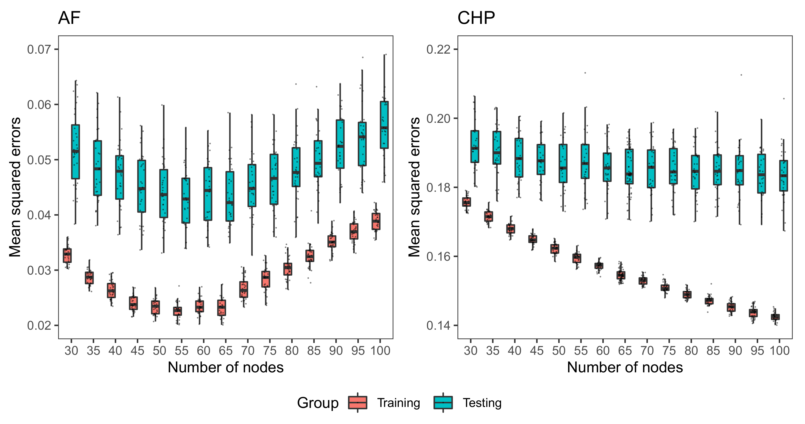
As illustrated in Figure 2, we investigate the performance of LLA with different number of nodes for testing and training data sets.
The left and right panels of Figure 2 depict the box-plots of MSEs for AF and CHP data sets, respectively. For CHP data, the MSE of training data decreases as the number of nodes increases, while the MSE of testing data decreases firstly and then remains at the same level as the number of nodes increases. This is expected since as the number of nodes increases, the corresponding neural network may be overfitted, which may lead to an increase of prediction error. For AF data set, the MSE of training and testing data decreases at first, but then increases as the number of nodes increases, reaching its minimum when the number of nodes is around 60. The difference in the pattern of training MSE between AF and CHP data in Figure 2 might be due to different sample sizes of AF data (n = 1503) and CHP data (n = 20,640).
Experiments of these two data sets suggest that LLA yields the best prediction performance when the number of nodes in one-hidden-layer neural network is 60. Thus, we set 60 as the default number of nodes for LLA regressor.
3.1.2. Comparison with Stochastic Gradient Algorithms
In this subsection, we compare the performance of LLA with Adam and Adamax [33], two popular stochastic gradient algorithms.
We consider default settings for these three algorithms. The default number of nodes in LLA is 60 by default, as discussed in Section 3.1.1. For the Adam algorithm, the default step size is , exponential decay rates for the moment estimates are , the constant for numerical stability is , and moving averages are initialized as zero vectors. The default settings for Adamax algorithm are the same as those of Adam, except that the step size is set to be .
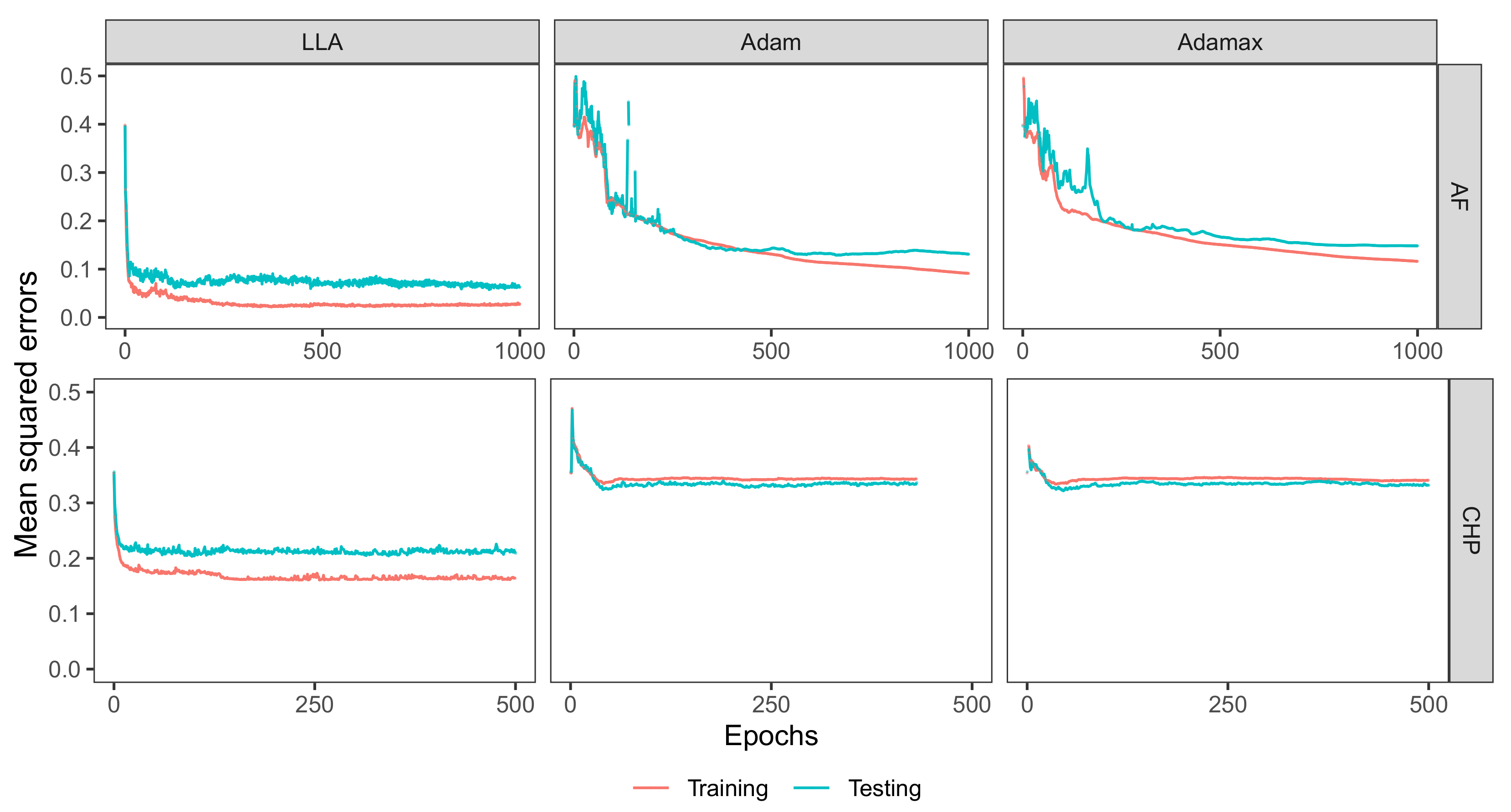
Figure 3 depicts the MSEs of training and testing data versus the number of epochs for each algorithm. From Figure 3, the MSEs of LLA algorithm become stable quickly after a few epochs. Compared with the Adam and the Adamax, the LLA algorithm needs fewer epochs to achieve stability. When the MSEs become stable, the LLA has the least MSEs among these three algorithms. This is expected because for a nonlinear least squares problem, the LLA algorithm utilizes both gradient and Hessian of the objective function in the minimization problem. In contrast, the Adam and Adamax algorithms are stochastic gradient descent algorithms, which only take advantage of the gradient of the objective function. Thus, they converge comparatively slowly.
3.1.3. Performance of LLA in Regression Settings
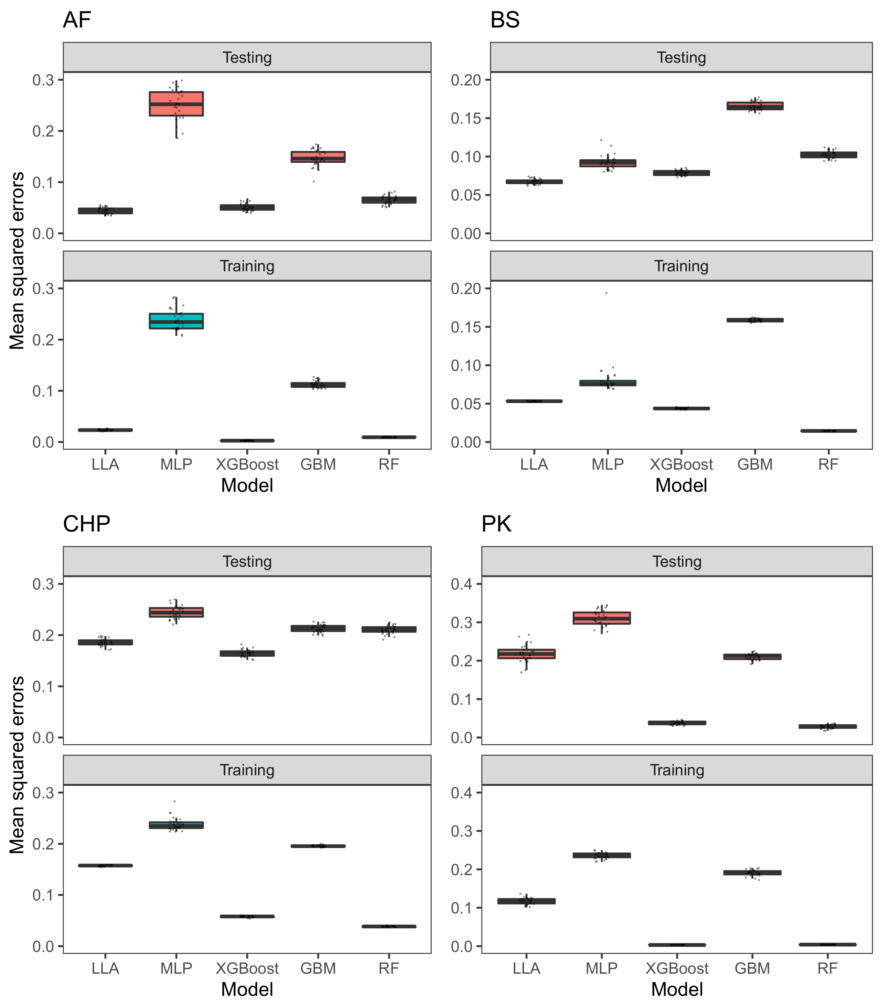
Next, we compare the performance of LLA with other commonly used procedures. All hyperparameters are set by default. However, the performance of procedures such as MLP might be further improved by extensively tuning their hyper-parameters. Table 1 depicts the values of 100 times of the sample mean and standard deviation of the 30 MSEs of testing data (testing MSE for short) as well as the 30 MSEs of training data (training MSE for short). Table 1 implies that XGBoost performs better than other two boosting methods: AdaBoost and GBM, and the LLA performs well in terms of prediction accuracy. Specifically, the LLA has the lowest testing MSEs for AF and BS data sets. For CHP, the LLA has slightly greater testing MSE than XGBoost, while XGBoost has a deeper tree by default. For AF, BS, and CHP data sets, the difference between testing MSE and training MSE is small for LLA. This implies that the LLA is less likely to be over-fitting. As illustrated in Figure 4, for AF, BS, and CHP data sets, the prediction MSE of MLP and GBM are likely to have large variation for different data splittings and thus more potential outliers. LLA prediction has relatively small standard deviation of MSEs and fewer points outside the interquartile range (IQR) of boxplots, compared to other procedures. This implies that LLA is likely to obtain consistent results and has a fairly stable performance. For PK data, LLA outperforms MLP in terms of both prediction accuracy and standard deviation of MSEs. However, XGBoost and RF have the best performance. This motivates us to examine the data further.
By doing exploratory data analysis of PK data, we find that several of the 19 predictors in PK data are highly correlated. For example, the correlation between Shimmer and Shimmer(dB) is 0.9923. The correlation between Jitter(%) and Jitter(RAP) is 0.9841. The poor performance of the LLA may be due to the collinearity of predictors since the linear regression is applied for updating the weights and biases. Thus, we conduct a principal component analysis (PCA), and the first 6, 9, and 13 principal components (PC) can explain 95%, 99%, and 99.9% of the variance. We further apply all procedures to PK data with predictors being set to PCs. Table 2 depicts the MSEs for PK data with PC predictors. Compared with Table 1, the performance of XGBoost and RF becomes poor. Table 1 and Table 2 imply that the performance of RF and XGBoost are not robust under linear transformation of predictors. The performance of MLP is quite stable across different numbers of PC variables. The performance of the LLA improves significantly via using PCs.
3.2. Classification
In this section, we compare the performance of LLA classifier with other commonly-used procedures based on the following three data sets.
(1) Ringnorm (RN, for short) data consists of n = 7400 observations with predictors and can be downloaded from https://www.cs.toronto.edu/~delve/data/ringnorm/desc.html (accessed on 15 January 2022). This data set has been analyzed in [41]. Each class is drawn from a multivariate normal distribution. Breiman [41] reports the theoretical expected misclassification rate as 1.3%.
(2) Magic gamma (MG, for short) data consists of n = 19,020 observations with predictors and can be downloaded from https://archive.ics.uci.edu/ml/datasets/MAGIC+Gamma+Telescope (accessed on 15 January 2022). The data are Monte Carlo generated to simulate registration of high energy gamma particles in a ground-based atmospheric Cherenkov gamma telescope using the imaging technique [42]. The binary response is whether the event is a signal or a background event. The explanatory variables include fLength (major axis of ellipse), fLength (minor axis of ellipse), fSize (10-log of sum of content of all pixels), fSize (ratio of sum of two highest pixels over fSize), fConc1 (ratio of highest pixel over fSize), fAsym (distance from highest pixel to center projected onto major axis), etc.
(3) Mammographic mass (MM, for short) data consists of observations with missing values deleted and predictors. It can be downloaded from https://archive.ics.uci.edu/ml/datasets/Mammographic+Mass (accessed on 15 January 2022). The response is severity (benign or malignant). The explanatory variables include age, shape, margin, and density.
We first standardize the continuous predictors so that their sample means and variances equal 0 and 1, respectively. We split each data set into 80% training data and 20% testing data with seed . Thus, we may obtain 30 AUC-ROC (AUC-ROC is the area under the receiver operating characteristic curve, which plots two parameters true positive rate and false positive rate. It provides an aggregate measure of performance of a classifier across all possible classification thresholds.) (AUC for short hereafter) scores for testing data and 30 AUC scores for training data for each procedure. We report the sample mean and standard deviation (std) of the 30 AUC scores for each procedure and data set.
3.2.1. Impact of the Number of Nodes for Classification Problems
We firstly investigate the impact of the number of nodes on the performance of LLA classifier in terms of AUCs for testing and training data sets. The number of nodes ranges from 15 to 70 in the LLA.
Figure 5 depicts the box-plots of AUCs for RN and MM data, respectively. For RN data set, the AUCs of training and testing data remain close to 1 across different number of nodes, and reach the maximum at approximately 30. As shown in Figure 5, when the number of nodes is small, LLA algorithm has a stable performance. As the number of nodes increases, it is likely to incur overfitting problem, especially for RN data set, leading to estimates with larger variance. For MM data, the AUCs of training data first increase and then keep constant when the number of nodes is chosen to be from 50 to 70. For the testing data, when the number of nodes varies from 15 to 35, the AUCs are close with each other. As the number of nodes increases, the AUCs for the testing data decrease and keep the same at approximately 0.85. When the number of nodes is too large, overfitting issue is likely to happen. As illustrated from these two data sets, when the number of nodes is set to be 30, the corresponding LLA classifier yields good performance in terms of prediction. Therefore, we set 30 as the default value in our numerical experiments for classification problems.
3.2.2. Comparison with Stochastic Gradient Algorithms
We then examine the convergence rate of the LLA algorithm in comparison with Adam and Adamax, two well-known stochastic gradient algorithms for neural networks. To make a fair comparison among the LLA, Adam and Adamax, we set in one-hidden-layer network for all these three algorithms. The default settings are used for the three algorithms. Specifically, the default step size for Adam is , the exponential decay rates for the moment estimates , . The constant for numerical stability is set to be . And the moving averages are initialized to be zero vectors. For Adamax, the step size is set to be .
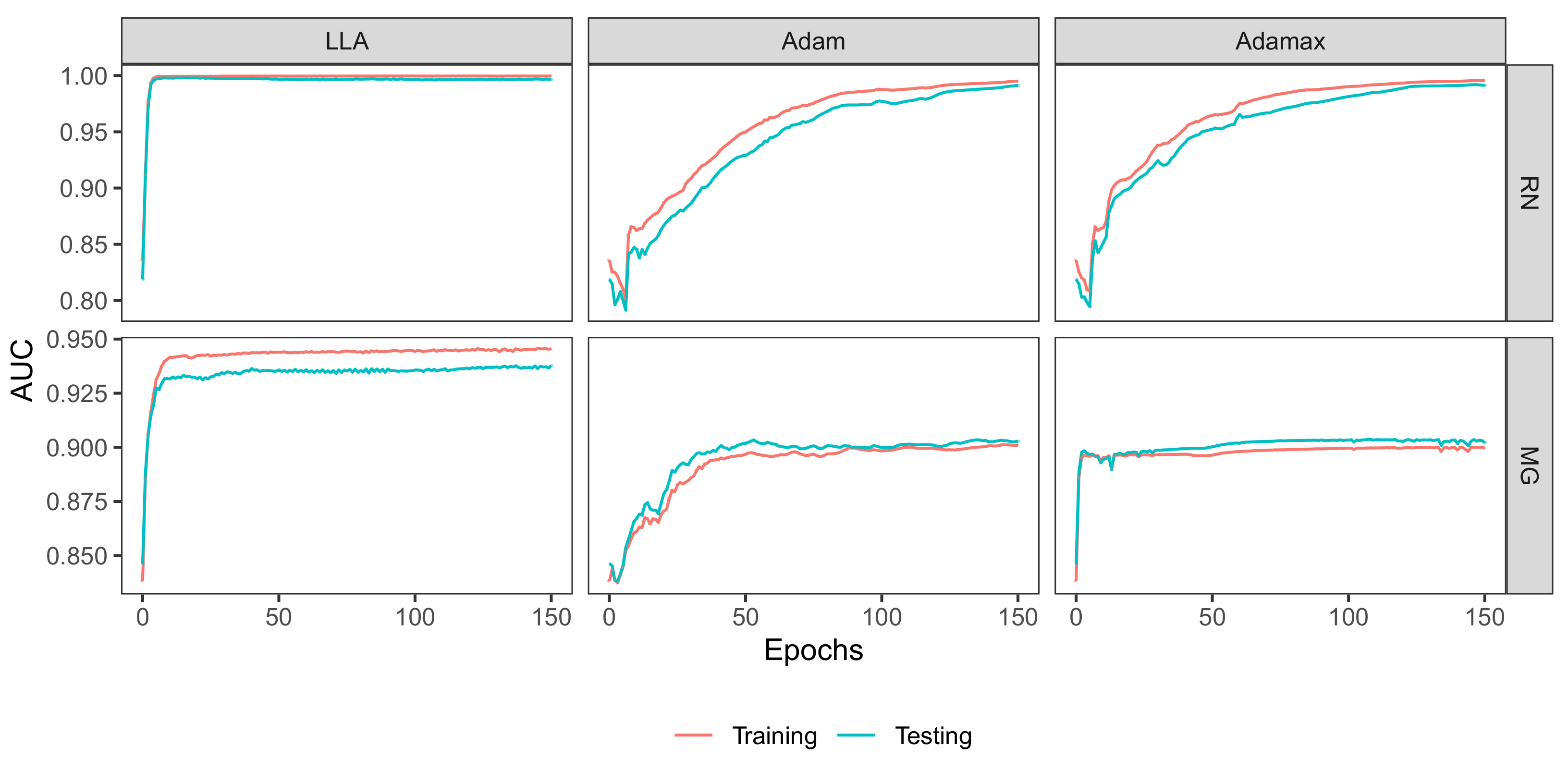
Figure 6 depicts the AUC scores of training and testing data versus the number of epochs for each algorithm. As seen from Figure 6, the AUC curves of the LLA algorithm increase and then become stable within 20 epochs for both RN and MG data sets. Both Adam and Adamax need many more epochs to have stable AUC values. For example, both Adam and Adamax need 150 epochs to have stable AUC values for RN data. This implies that the LLA converges faster than Adam and Adamax, consistent with our theoretical analysis. The LLA also performs better than the Adam and Adamax in terms of AUC score. This can be clearly seen from the AUC plots for the MG data set.
3.2.3. Performance of LLA in Classification Problems
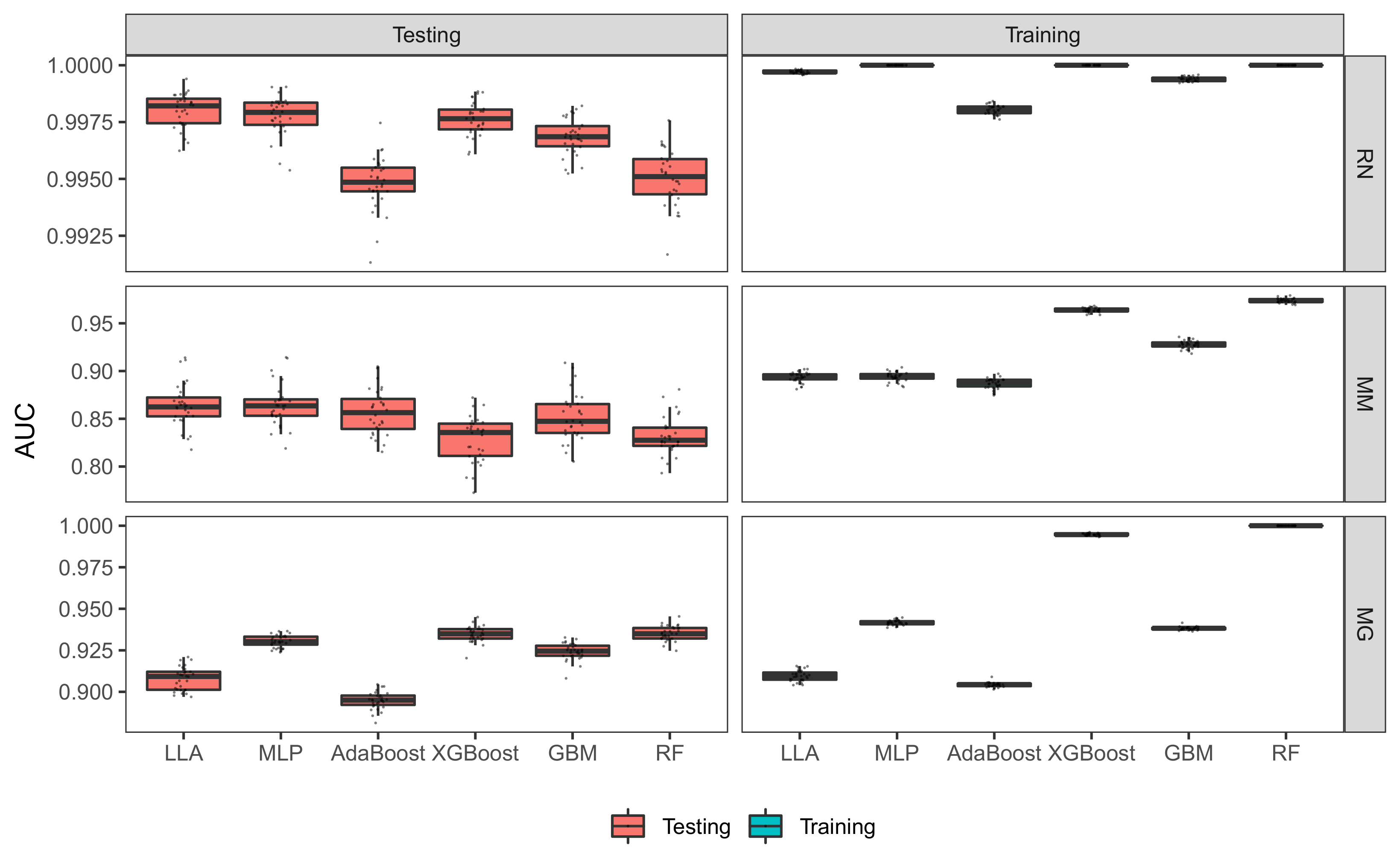
We next compare the performance of the LLA classifier with other procedures with default settings. The number of nodes in the LLA for RN, MM and MG data sets are 30. The number of max epochs is set to be 100. Table 3 depicts the values of 100 times of the sample mean and standard deviations of the 30 AUC scores for the testing data (testing AUC for short) as well as those for the training data (training AUC for short). Table 3 implies that the LLA performs the best for RN and MM data sets in terms of AUC scores, followed by MLP. Figure 7 compares the AUC scores of different methods more explicitly. As shown in Figure 7, all procedures have small standard deviation for the testing data. However, for the training data, RF has a large standard deviation for the RN data while XGBoost, GBM, and Adaboost have more fluctuations for the MM data. The LLA has small standard deviations for all data sets, illustrating that the LLA retains stability. The differences between the testing AUCs and training AUCs are small for the LLA classifier, which shows that it is less likely for the LLA classifier to be over-fitting. For MG data, the RF performs the best, followed by XGBoost. This motivates us to examine the data further by considering multi-layer network, which will be discussed in Section 3.4 in details.
3.3. Analysis of Computational Time
In this section, we compare the computational time of LLA with other commonly used procedures. As shown in Figure 3, LLA converges faster than ADAM algorithm in terms of training epochs. Each training epoch of LLA takes longer time than Adam and Adamax, though. To make fair comparison on computational time, we use the ‘tensorflow.keras.Sequential’ to build one-hidden-layer neural networks with Adam and Adamax optimizers. Similar to the Monte Carlo experiment settings used for Table 1 and Table 3, we randomly split the data into two parts (80% for training and 20% for testing), and repeat the process for 30 times to calculate the mean and standard deviation. For regression problems, models contain 60 nodes (by default) in the hidden layer and are forced to run 1000 epochs. For classification problems, models contain 30 nodes (by default) in the hidden layer and are forced to run 150 epochs. The experiments are run on a personal computer (3.1 GHz Intel Core i5 processor) with Python 3.8 and TesorFlow 2.4.0. Table 4 shows the sample means along with standard deviations (in parenthesis) of testing MSE (100 times of the actual values), and training time (in seconds). The results show that although LLA takes longer time in training 1000/150 epochs, it can achieve higher accuracy in both regression and classification models. Moreover, as shown in Figure 3 and Figure 6, LLA converges in fewer epochs than Adam or Adamax, demonstrating that if early stopping is applied, computational time of LLA is comparable to the time of Adam and Adamax. Consider AF data set as an example. If LLA stops at 220 epochs, its average and standard deviation of training time will be 55.3 and 9.2 s, meaning that the computational time of LLA is close to Adam’s and Adamax’s. For classification problems, LLA can also converge in fewer epochs than Adam or Adamax as shown in Figure 6.
3.4. Performance of Deep LOAN
In this subsection, we examine the performance of the LOAN with multiple-hidden layers. Since there is no option to set different depth levels for AdaBoost, we exclude it for this comparison. We set the MLP, XGBoost, GBM, and RF with the same number of layer or depth as L, the number of hidden layers used in the LLA. Other parameters of the MLP, XGBoost, GBM and RF are set to be the default values. For regression problem, we apply these four procedures and LLA to CHP data. For classification problem, we investigate MG data in details.
For regression problems, Table 5 depicts the sample mean and standard deviation of the 30 training and testing data splittings for , 2 and 3, based on CHP data set. The number of nodes in the one-hidden-layer LOAN is set to be 60. The number of nodes in the LOAN with two hidden layer is set to be 60 and 10 in the first and second layer, respectively. The number of nodes in the LOAN with three hidden layers is set to be 60, 10, and 50 in the first, second and third layer, respectively. From Table 5, we can see that both the LOAN and MLP have smaller MSE as L increases, but there is no dramatic improvement, while XGBoost, GBM, and RF seem to have more improvement as L increases. Table 5 indicates that LOAN performs the best when 2 and 3 in terms of mean and standard deviation of both training and testing MSEs.
For classification problems, Table 6 depicts the sample means and standard deviations of AUC scores for different values of L based on MG data set. For LOAN with different number of layers, 30 nodes is chosen for each layer. Compared with GBM and RF, LLA, MLP, and XGBoost perform better. As the number of layer increases, the improvement of LOAN is dramatic. Although LLA does not perform the best when only one hidden layer is used, it achieves the highest AUC scores when L is set to be 2 and 3. The standard deviations for LOAN continue to decrease as L increases for both testing and training data, illustrating that deep LLA leads to a more stable performance in terms of prediction for this data set. These experiments demonstrate that shallow LOAN achieves both stable performance and high prediction accuracy level compared to commonly-used deep learning models.
4. Conclusions and Discussion
In this paper, we develop the LLA algorithm in an FNN for both regression and classification problems, and show that the LLA has a quadratic convergence rate. Our comparison based on benchmark data sets indicates that the LLA can greatly improve training efficiency and outperforms commonly-used procedures in both training time and prediction accuracy. This algorithm is generally applicable, and can be extended to deep neural networks via layer-wise or back-propagation construction. Exciting future work could further extend the proposed method in different studies such as survival data analysis. Parallel computing algorithm can also be developed for the proposed method.
Author Contributions
R.L. and A.S. proposed the topic and framework. M.Z. and Y.L. implemented the algorithm and conducted real data analysis. All authors have read and agreed to the published version of the manuscript.
Funding
This research received no external funding.
Data Availability Statement
The data analyzed in Section 3.1 and Section 3.2 are publicly available.
Acknowledgments
The authors are grateful to the reviewers for constructive comments, which lead to a significant improvement of this work. The views expressed in the paper are those of the authors and do not represent the views of Wells Fargo.
Conflicts of Interest
The authors declare no conflict of interest.
Appendix A
This appendix consists of the proofs of Theorems 1 and 2.
Appendix A.1. Proof of Theorem 1
Proof.
Recall . Thus, the corresponding least squares problem is
The Fisher scoring algorithm is to update
The gradient and Hessian matrix of the least squares function can be derived
Thus,
and a natural estimate of is
Then
By using Fisher scoring algorithm, we do not need to evaluate , which typically is hard to calculate. The LLA is to approximate by
Note that
and
Thus,
Therefore, the Fisher scoring algorithm for the least squares function based on the local linear approximation
has the same updated as given in (A1). This completes the proof of Theorem 1. □
Appendix A.2. Proof of Theorem 2
References
- Gardner, W.A. Learning characteristics of stochastic-gradient-descent algorithms: A general study, analysis, and critique. Signal Process. 1984, 6, 113–133. [Google Scholar] [CrossRef]
- Oymak, S.; Soltanolkotabi, M. Overparameterized nonlinear learning: Gradient descent takes the shortest path? In Proceedings of the 36th International Conference on Machine Learning (ICML), PMLR, Long Beach, CA, USA, 9–15 June 2019; Volume 97, pp. 4951–4960. [Google Scholar]
- Ali, A.; Dobriban, E.; Tibshirani, R. The implicit regularization of stochastic gradient flow for least squares. In Proceedings of the 37th International Conference on Machine Learning (ICML), PMLR, Virtual, 13–18 July 2020; pp. 233–244. [Google Scholar]
- Douglas, S.; Meng, T.Y. Linearized least-squares training of multilayer feedforward neural networks. In Proceedings of the IJCNN-91-Seattle International Joint Conference on Neural Networks, Seattle, WA, USA, 8–12 July 1991; Volume 1, pp. 307–312. [Google Scholar] [CrossRef]
- Singhal, S.; Wu, L. Training multilayer perceptrons with the extende kalman algorithm. Adv. Neural Inf. Process. Syst. 1988, 1, 133–140. [Google Scholar]
- Stan, O.; Kamen, E. A local linearized least squares algorithm for training feedforward neural networks. IEEE Trans. Neural Netw. 2000, 11, 487–495. [Google Scholar] [CrossRef] [PubMed]
- Kollias, S.; Anastassiou, D. An adaptive least squares algorithm for the efficient training of artificial neural networks. IEEE Trans. Circuits Syst. 1989, 36, 1092–1101. [Google Scholar] [CrossRef]
- Ngia, L.S.; Sjoberg, J. Efficient training of neural nets for nonlinear adaptive filtering using a recursive Levenberg-Marquardt algorithm. IEEE Trans. Signal Process. 2000, 48, 1915–1927. [Google Scholar] [CrossRef]
- Kim, C.T.; Lee, J.J. Training two-layered feedforward networks with variable projection method. IEEE Trans. Neural Netw. 2008, 19, 371–375. [Google Scholar]
- Zhou, G.; Si, J. Advanced neural-network training algorithm with reduced complexity based on Jacobian deficiency. IEEE Trans. Neural Netw. 1998, 9, 448–453. [Google Scholar] [CrossRef] [PubMed]
- Maddox, W.; Tang, S.; Moreno, P.; Wilson, A.G.; Damianou, A. Fast adaptation with linearized neural networks. In Proceedings of the 24th International Conference on Artificial Intelligence and Statistics, PMLR, Virtual, 13–15 April 2021; Volume 130, pp. 2737–2745. [Google Scholar]
- Khan, M.E.; Immer, A.; Abedi, E.; Korzepa, M. Approximate inference turns deep networks into Gaussian processes. arXiv 2019, arXiv:1906.01930. [Google Scholar]
- Mu, F.; Liang, Y.; Li, Y. Gradients as features for deep representation learning. In Proceedings of the 8th International Conference on Learning Representations (ICLR), Addis Ababa, Ethiopia, 26–30 April 2020. [Google Scholar]
- Jacot, A.; Gabriel, F.; Hongler, C. Neural tangent kernel: Convergence and generalization in neural networks. In Advances in Neural Information Processing Systems; Bengio, S., Wallach, H., Larochelle, H., Grauman, K., Cesa-Bianchi, N., Garnett, R., Eds.; Curran Associates, Inc.: Red Hook, NY, USA, 2018; Volume 31, pp. 8571–8580. [Google Scholar]
- Martens, J. Deep learning via hessian-free optimization. In Proceedings of the 27th International Conference on Machine Learning (ICML), Haifa, Israel, 21–24 June 2010; pp. 735–742. [Google Scholar]
- Kunstner, F.; Balles, L.; Hennig, P. Limitations of the empirical fisher approximation for natural gradient descent. arXiv 2020, arXiv:1905.12558v3. [Google Scholar]
- Hornik, K.; Stinchcombe, M.; White, H. Multilayer feedforward networks are universal approximators. Neural Netw. 1989, 2, 359–366. [Google Scholar] [CrossRef]
- Cybenko, G. Approximation by superpositions of a sigmoidal function. Math. Control. Signals Syst. 1989, 2, 303–314. [Google Scholar] [CrossRef]
- Goodfellow, I.; Bengio, Y.; Courville, A. Deep Learning; MIT Press: Cambridge, UK, 2016; Volume 1. [Google Scholar]
- Huang, G.B.; Zhu, Q.Y.; Siew, C.K. Extreme learning machine: Theory and applications. Neurocomputing 2006, 70, 489–501. [Google Scholar] [CrossRef]
- Yu, D.; Deng, L. Efficient and effective algorithms for training single-hidden-layer neural networks. Pattern Recognit. Lett. 2012, 33, 554–558. [Google Scholar] [CrossRef]
- Kurita, T. Iterative weighted least squares algorithms for neural networks classifiers. New Gener. Comput. 1994, 12, 375–394. [Google Scholar] [CrossRef]
- Martens, J. New Insights and Perspectives on the Natural Gradient Method. J. Mach. Learn. Res. 2020, 21, 1–76. [Google Scholar]
- Hinton, G.E. Training products of experts by minimizing contrastive divergence. Neural Comput. 2002, 14, 1771–1800. [Google Scholar] [CrossRef]
- Bengio, Y.; Lamblin, P.; Popovici, D.; Larochelle, H. Greedy layer-wise training of deep networks. Adv. Neural Inf. Process. Syst. 2007, 19, 153. [Google Scholar]
- Bengio, Y.; Delalleau, O. Justifying and generalizing contrastive divergence. Neural Comput. 2009, 21, 1601–1621. [Google Scholar] [CrossRef]
- Hinton, G.E. Learning multiple layers of representation. Trends Cogn. Sci. 2007, 11, 428–434. [Google Scholar] [CrossRef]
- Salakhutdinov, R.; Hinton, G. Deep boltzmann machines. In Proceedings of the 12th International Conference on Artificial Intelligence and Statistics, PMLR, Clearwater Beach, FL, USA, 16–18 April 2009; Volume 5, pp. 448–455. [Google Scholar]
- Jaderberg, M.; Czarnecki, W.M.; Osindero, S.; Vinyals, O.; Graves, A.; Silver, D.; Kavukcuoglu, K. Decoupled neural interfaces using synthetic gradients. In Proceedings of the 34th International Conference on Machine Learning, PMLR, Sydney, Australia, 6–11 August 2017; Volume 70, pp. 1627–1635. [Google Scholar]
- Chen, S.; Wang, W.; Pan, S.J. Deep neural network quantization via layer-wise optimization using limited training data. In Proceedings of the AAAI Conference on Artificial Intelligence, Honolulu, HI, USA, 27 January–1 February 2019; Volume 33, pp. 3329–3336. [Google Scholar]
- Shin, Y. Effects of depth, width, and initialization: A convergence analysis of layer-wise training for deep linear neural networks. arXiv 2019, arXiv:1910.05874. [Google Scholar] [CrossRef]
- Song, Y.; Meng, C.; Liao, R.; Ermon, S. Nonlinear equation solving: A faster alternative to feedforward computation. arXiv 2020, arXiv:2002.03629. [Google Scholar]
- Kingma, D.P.; Ba, J. Adam: A Method for Stochastic Optimization. arXiv 2017, arXiv:1412.6980v9. [Google Scholar]
- Pal, S.K.; Mitra, S. Multilayer perceptron, fuzzy sets, classifiaction. IEEE Trans. Neural Netw. 1992, 3, 683–697. [Google Scholar] [CrossRef] [PubMed]
- Pedregosa, F.; Varoquaux, G.; Gramfort, A.; Michel, V.; Thirion, B.; Grisel, O.; Blondel, M.; Prettenhofer, P.; Weiss, R.; Dubourg, V.; et al. Scikit-learn: Machine learning in Python. J. Mach. Learn. Res. 2011, 12, 2825–2830. [Google Scholar]
- Chen, T.; Guestrin, C. Xgboost: A scalable tree boosting system. In Proceedings of the 22nd ACM SIGKDD International Conference on Knowledge Discovery and Data Mining, San Francisco, CA, USA, 13–17 August 2016; pp. 785–794. [Google Scholar]
- Friedman, J.H. Greedy function approximation: A gradient boosting machine. Ann. Stat. 2001, 29, 1189–1232. [Google Scholar] [CrossRef]
- Freund, Y.; Schapire, R.E. A decision-theoretic generalization of on-line learning and an application to boosting. J. Comput. Syst. Sci. 1997, 55, 119–139. [Google Scholar] [CrossRef] [Green Version]
- Breiman, L. Random forests. Mach. Learn. 2001, 45, 5–32. [Google Scholar] [CrossRef] [Green Version]
- Pace, R.K.; Barry, R. Sparse spatial autoregressions. Stat. Probab. Lett. 1997, 33, 291–297. [Google Scholar] [CrossRef]
- Breiman, L. Bias, Variance, and Arcing Classifiers; Technical Report, 460; Statistics Department, University of California: Berkeley, CA, USA, 1996. [Google Scholar]
- Heck, D.; Knapp, J.; Capdevielle, J.; Schatz, G.; Thouw, T. CORSIKA: A Monte Carlo code to simulate extensive air showers. Rep. Fzka 1998, 6019, 5–8. [Google Scholar]
Figure 1.
Illustration of LLA in Equation (4). The LLA algorithm is to approximate by a local linear function iteratively, where t stands for a general argument and is replaced with in the text. This figure illustrates the LLA of the ReLU activation function at points A, B and C with local linear functions around their neighborhood.

Figure 2.
Box plots of 30 MSEs of one-hidden-layer LLA with nodes for training and testing data. The left panel is for the AF data set and the right panel is for the CHP data set.
Figure 2.
Box plots of 30 MSEs of one-hidden-layer LLA with nodes for training and testing data. The left panel is for the AF data set and the right panel is for the CHP data set.

Figure 3.
MSE of LLA, Adam and Adamax algorithms versus the number of epochs.

Figure 4.
Comparison with commonly-used procedures with default hyper-parameter value for regression problems.
Figure 4.
Comparison with commonly-used procedures with default hyper-parameter value for regression problems.

Figure 5.
Box plots of 30 AUCs of LLA algorithm with nodes being set to for training and testing data. The top panel is the AUCs of RN data set, and the bottom panel is the AUCs of MM data set.
Figure 5.
Box plots of 30 AUCs of LLA algorithm with nodes being set to for training and testing data. The top panel is the AUCs of RN data set, and the bottom panel is the AUCs of MM data set.

Figure 6.
AUCs of LLA, Adam and Adamax algorithms versus the number of epochs.

Figure 7.
Box plots of 30 AUCs for the LLA and the five commonly-used procedures with default hyper-parameter values for classification problems.
Figure 7.
Box plots of 30 AUCs for the LLA and the five commonly-used procedures with default hyper-parameter values for classification problems.


Table 1.
Comparison with commonly-used regressors with default hyper-parameter values.
| Methods | AF | BS | CHP | PK |
|---|---|---|---|---|
| 100 × Mean (Std) | 100 × Mean (Std) | 100 × Mean (Std) | 100 × Mean (Std) | |
| MSE for Testing Data | ||||
| LLA | 4.3317 (0.5895) | 6.7291 (0.2957) | 18.5801 (0.6955) | 22.8113 (5.4049) |
| MLP | 25.4913 (3.4600) | 9.9173 (2.0827) | 24.1495 (1.0754) | 31.4595 (2.3832) |
| XGBoost | 5.1042 (0.7245) | 7.8751 (0.3137) | 16.4491 (0.6905) | 3.7880 (0.4386) |
| AdaBoost | 31.7242 (2.6197) | 27.7419 (0.7384) | 56.3744 (5.3267) | 60.9171 (1.8358) |
| GBM | 14.7338 (1.5846) | 16.5968 (0.5592) | 21.2866 (0.7254) | 21.0340 (0.7685) |
| RF | 6.5254 (0.7346) | 10.2843 (0.4672) | 21.2067 (0.9217) | 2.8041 (0.4835) |
| MSE for Training Data | ||||
| LLA | 2.3213 (0.1634) | 5.3265 (0.0828) | 15.7216 (0.1275) | 11.7173 (0.8164) |
| MLP | 24.5284 (0.0268) | 7.7488 (0.7496) | 23.7055 (1.1570) | 23.7447 (1.3502) |
| XGBoost | 0.2623 (0.0268) | 4.3713 (0.0946) | 5.7634 (0.1456) | 0.3115 (0.0264) |
| AdaBoost | 29.2881 (1.1124) | 27.2715 (0.6059) | 55.8631 (5.5463) | 60.4119 (1.1948) |
| GBM | 11.2280 (0.6303) | 15.8681 (0.1972) | 19.5493 (0.1864) | 19.0881 (0.7516) |
| RF | 0.9366 (0.0388) | 1.4413 (0.0179) | 3.8432 (0.0766) | 0.3897 (0.0356) |
Table 2.
Comparison of the impact of PCA on LLA and existing procedures based on PK data.
| Methods | 6 PCs | 9 PCs | 13 PCs | All (19) PCs |
|---|---|---|---|---|
| 100 × Mean (Std) | 100 × Mean (Std) | 100 × Mean (Std) | 100 × Mean (Std) | |
| MSE for Testing Data | ||||
| LLA | 23.1102 (2.1758) | 9.3551 (0.9400) | 10.2220 (1.1961) | 22.2247 (3.0623) |
| MLP | 41.7293 (2.6673) | 34.7943 (2.3511) | 30.6869 (2.1018) | 30.6617 (2.9831) |
| XGBoost | 50.8823 (3.2462) | 47.1367 (2.7843) | 42.9631 (2.6408) | 44.4751 (2.1000) |
| AdaBoost | 81.2930 (2.6109) | 78.9303 (2.7339) | 76.2363 (2.2727) | 76.5351 (2.5682) |
| GBM | 67.0713 (2.3618) | 62.4927 (2.2980) | 59.1466 (1.8239) | 59.7928 (1.9610) |
| RF | 41.2433 (2.8571) | 39.6862 (2.6231) | 37.7282 (2.5413) | 39.9511 (2.5392) |
| MSE for Training Data | ||||
| LLA | 17.0868 (1.2977) | 5.8743 (0.3081) | 5.8837 (0.5092) | 11.7854 (0.8391) |
| MLP | 37.1915 (1.8439) | 27.9013 (0.9417) | 22.0252 (0.9036) | 20.5078 (0.9063) |
| XGBoost | 10.0009 (0.7694) | 6.6056 (0.4240) | 4.0770 (0.3162) | 2.9568 (0.2952) |
| AdaBoost | 79.1353 (2.3975) | 76.3020 (2.1195) | 73.5840 (2.0781) | 73.5073 (2.3712) |
| GBM | 59.1133 (1.5346) | 53.7506 (1.1314) | 49.5714 (0.9834) | 49.4500 (0.9870) |
| RF | 5.9341 (0.2602) | 5.6795 (0.1998) | 5.3804 (0.2432) | 5.6393 (0.2185) |
Table 3.
Comparison with commonly-used classifiers with default hyper-parameters value.
| Methods | RN | MM | MG |
|---|---|---|---|
| 100 × Mean (Std) | 100 × Mean (Std) | 100 × Mean (Std) | |
| AUC Scores for Testing Data | |||
| LLA | 99.8007 (0.0750) | 86.4075 (2.3068) | 90.7903 (0.6989) |
| MLP | 99.7777 (0.0856) | 86.3424 (2.1636) | 93.0479 (0.3572) |
| XGBoost | 99.7641 (0.0723) | 82.8425 (2.4301) | 93.4792 (0.4691) |
| AdaBoost | 99.4795 (0.1202) | 85.6732 (2.3398) | 89.4802 (0.5192) |
| GBM | 99.6859 (0.0793) | 85.2137 (2.5059) | 92.4214 (0.5086) |
| RF | 99.5045 (0.1249) | 83.2001 (1.9674) | 93.5235 (0.4453) |
| AUC Scores for Training Data | |||
| LLA | 99.9705 (0.0072) | 89.3458 (0.5252) | 90.9545 (0.3217) |
| MLP | 100.0000 (0.0000) | 89.4176 (0.4736) | 94.1618 (0.1429) |
| XGBoost | 100.0000 (0.0000) | 96.3674 (0.2275) | 99.4716 (0.0675) |
| AdaBoost | 99.8049 (0.0199) | 88.7022 (0.5184) | 90.4314 (0.1327) |
| GBM | 99.9389 (0.0097) | 92.7635 (0.4055) | 93.8208 (0.0975) |
| RF | 100.0000 (0.0000) | 97.3740 (0.2280) | 100.0000 (0.0000) |
Table 4.
Training time and accuracy (testing MSE/AUC for regression/classification problems) of LLA, Adam, and Adamax. For AF and CHP (regression) data sets, the training epoch is fixed at 1000. For RN and MG (classification) data sets, the training epoch is fixed at 150. MSE(std) and AUC(std) in this table denote 100 times of the average(standard deviation) of MSE/AUC values over epochs. Time is measured in seconds.
| Data | LLA | Adam | Adamax | |
|---|---|---|---|---|
| AF | MSE (std) | 4.6 (0.6) | 25.2 (4.0) | 24.3 (3.2) |
| Time (std) | 207.3 (12.6) | 58.8 (5.1) | 49.3 (5.2) | |
| CHP | MSE (std) | 18.8 (0.7) | 24.9 (1.2) | 23.8 (0.1) |
| Time (std) | 998.9 (190.1) | 407.3 (80.6) | 397.2 (77.4) | |
| RN | AUC (std) | 99.8 (0.1) | 99.6 (0.2) | 99.6 (0.0) |
| Time (std) | 101.2 (1.7) | 26.8 (1.4) | 24.1 (0.9) | |
| MG | AUC (std) | 91.8 (0.7) | 91.9 (0.0) | 91.7 (0.1) |
| Time (std) | 122.8 (2.3) | 68.0 (2.9) | 59.1 (3.9) |
Table 5.
Comparison of the number of hidden layers in LOAN and existing regressors based on CHP data.
Table 5.
Comparison of the number of hidden layers in LOAN and existing regressors based on CHP data.
| Methods | |||
|---|---|---|---|
| 100 × Mean (Std) | 100 × Mean (Std) | 100 × Mean (Std) | |
| MSE for Testing Data | |||
| LOAN | 18.580 (0.696) | 18.016 (0.674) | 17.524 (0.653) |
| MLP | 22.538 (0.967) | 20.627 (0.896) | 20.232 (0.876) |
| XGBoost | 28.537 (0.777) | 20.796 (0.661) | 18.340 (0.652) |
| GBM | 35.532 (0.869) | 24.591 (0.745) | 21.287 (0.726) |
| RF | 66.745 (1.496) | 53.697 (1.151) | 43.940 (1.096) |
| MSE for Training Data | |||
| LOAN | 15.722 (0.128) | 14.365 (0.243) | 12.555 (0.157) |
| MLP | 21.272 (0.656) | 18.353 (0.472) | 16.737 (0.543) |
| XGBoost | 27.909 (0.183) | 19.150 (0.242) | 15.127 (0.167) |
| GBM | 35.161 (0.196) | 23.762 (0.210) | 19.549 (0.186) |
| RF | 66.707 (0.609) | 53.538 (0.333) | 43.483 (0.329) |
Table 6.
Comparison of the number of hidden layers in LOAN and existing classifiers based on MG data.
Table 6.
Comparison of the number of hidden layers in LOAN and existing classifiers based on MG data.
| Methods | |||
|---|---|---|---|
| 100 × Mean (Std) | 100 × Mean (Std) | 100 × Mean (Std) | |
| AUC for Testing Data | |||
| LLA | 90.7903 (0.6989) | 93.8978 (0.3857) | 94.3385 (0.3556) |
| MLP | 92.6980 (0.3915) | 93.0171 (0.4185) | 92.8342 (0.5058) |
| XGBoost | 89.5843 (0.6247) | 92.4452 (0.4989) | 93.2186 (0.4459) |
| GBM | 87.8336 (0.6711) | 91.4000 (0.5723) | 92.4214 (0.5087) |
| RF | 82.2163 (1.1715) | 86.5378 (0.6972) | 87.6666 (0.6656) |
| AUC for Training Data | |||
| LLA | 90.9545 (0.3217) | 95.2309 (0.1458) | 96.9006 (0.1088) |
| MLP | 93.3201 (0.1632) | 94.7166 (0.1804) | 95.6310 (0.2325) |
| XGBoost | 90.2653 (0.1400) | 93.8429 (0.1111) | 95.6249 (0.0967) |
| GBM | 88.2751 (0.1475) | 92.2619 (0.1215) | 93.8208 (0.0975) |
| RF | 82.4167 (0.6175) | 86.8213 (0.2831) | 88.0429 (0.1949) |
Publisher’s Note: MDPI stays neutral with regard to jurisdictional claims in published maps and institutional affiliations. |
© 2022 by the authors. Licensee MDPI, Basel, Switzerland. This article is an open access article distributed under the terms and conditions of the Creative Commons Attribution (CC BY) license (https://creativecommons.org/licenses/by/4.0/).
Share and Cite
MDPI and ACS Style
Zeng, M.; Liao, Y.; Li, R.; Sudjianto, A. Local Linear Approximation Algorithm for Neural Network. Mathematics 2022, 10, 494. https://0-doi-org.brum.beds.ac.uk/10.3390/math10030494
AMA Style
Zeng M, Liao Y, Li R, Sudjianto A. Local Linear Approximation Algorithm for Neural Network. Mathematics. 2022; 10(3):494. https://0-doi-org.brum.beds.ac.uk/10.3390/math10030494
Chicago/Turabian StyleZeng, Mudong, Yujie Liao, Runze Li, and Agus Sudjianto. 2022. "Local Linear Approximation Algorithm for Neural Network" Mathematics 10, no. 3: 494. https://0-doi-org.brum.beds.ac.uk/10.3390/math10030494
Note that from the first issue of 2016, this journal uses article numbers instead of page numbers. See further details here.