Fundamentals vs. Financialization during Extreme Events: From Backwardation to Contango, a Copper Market Analysis during the COVID-19 Pandemic

Abstract

The COVID-19 pandemic has shocked commodities markets in general and base metals markets in particular. The market turmoil made it very difficult to act in the physical market, given the impossibility of establishing or maintaining physical and/or financial positions in a context of high uncertainty. This has happened both in different moments of the development of the pandemic and in geographically different frames. That is why this contribution tries to explain the evolution of warehouses and copper price structure and its utility for hedging in the context of an extreme event. To that end, Granger causality has been used to test whether, during the COVID-19 first wave, the pandemic evolution is cointegrated on one hand with copper futures price structure and, on the other, with the incremental levels of copper stocks. Using 102 official copper prices on London Metal Exchange (LME) trading days, between 13 January 2020 and 5 June 2020 (once the most severe effects of the first wave had been overcome), it was demonstrated that, during the first COVID-19 wave in Europe, the weekly death index variation was cointegrated with the copper future price structure. It has been proven that, in this timelapse, contango in futures price structure has increased its value, and the incremental levels of stock in copper LME warehouses are linked with a stable contango structure. In short, we find that fundamental market effects predominate, in a context in which commodities used to be more financialized. This leads market players, such as traders, miners, and transformers, to move exposures in their hedging structures, under such extreme event situations, in favor of or against either contango or backwardation, so as to derive value from them.

1. Introduction

The COVID-19 pandemic started as an epidemic, with China being the first country reporting the disease. It was only 100 days until the declaration of the pandemic. After that, governments in every country implemented different measures to control the crisis, with a common structure: social distancing, lockdowns, stay-at-home orders, and travel restrictions, all of which had economic impacts. The whole world experienced a period in which the economy was not running efficiently, causing some businesses to collapse.

The recovery after the emergence of the pandemic evolved differently depending on the country and the sanitary situation, causing a global disruption in the commerce interchange and affecting the full value-added chain.

Commodities market prices reached their lowest level in decades, such as, for example, the crude oil and natural gas markets [1]. Other commodities traded in futures exchanges, such as soft commodities and metals, also reacted sharply to this global crisis, with a vast shift in prices [2], and the historical refuges of these stock markets also being affected [3]. Copper, in particular, underwent a price decrease of almost 25%, from EUR 6200 at the beginning of 2020 to EUR 4627 per metric ton only 3 months after, with a lack of interest in the buying market and with most of the players trying to liquidate their long-held positions in official warehouses.

This COVID-19 pandemic has had by far the biggest influence on every market in recent times when base metals prices on commodities exchanges have been influenced by macroeconomic and microeconomic events. Each of these base metals shows different behaviors depending on its supply–demand situation, and how financialized each is.

Microeconomic and macroeconomic events have influenced commodities’ behaviors in different exchanges. Some of these macroeconomics variables, such as Gross Domestic Product (GDP), have been used to determine the effects on the 27 commodity futures traded on the Commodity Research Bureau (CRB) [4], and the effect on the S&P 500 index has been tested using commodity price indexes [5]. It is also informative to study currency volatility and the link between currency rates for 17 soft and hard commodities [6]. Crude oil prices have also been analyzed by some authors, who found a vast range of variables affecting prices, such as the COVID-19 outbreak, the USD index, and Pacific Investment Management Company (PIMCO) Investment Grade Corporate bond index [7], and US and BRICS (Brazil, Russia, India, China and South Africa) equities [8]. Globally, it has been demonstrated that price cycles are affected by macroeconomic variables [9].

The increase in financialization on the commodity market has been observable for a while [10,11], with commodities in general and base metals in particular being a refuge for investors trying to hedge their global exposure. In this regard, 2004 was pinpointed by some authors [12] as the year in which financialization became more present, ultimately achieving inflows of up to USD 450 billion seven years later in 2011 [13].

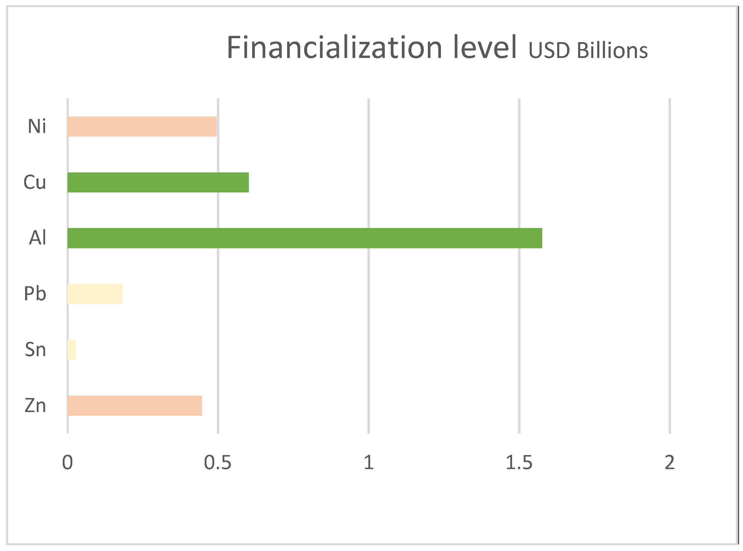
Specifically, we find that copper and aluminum are the two most highly financialized base metals, following the LME’s (London Metal Exchange) Commitment of Traders Report (see Figure 1).

The so-called “normal backwardation” theory links the fundamental scarcity level of a commodity (physical supply and demand) with the appearance of a higher price in the short term than in the long term. This was first studied by [14], looking generally at commodities [15] and specifically at certain metals such as zinc [16], and some have recently assessed financialization factors [17]. Several trends in the data also reflect the disappearance of “normal backwardation” in specific periods of study and in different commodities [18,19].

The theory of normal backwardation is also established through the theory of storage and is related to the cost of carry (COC) model, as shown in [20], where it was shown that risk premium could be used to determine a long-term pricing model. This theory of storage was used to study the levels of stocks in warehouses in different exchanges, which has always been one of the main factors of the fundamentals-based movements of contango and backwardation. The literature addressing this theory is broad [21,22,23], and a model combining backwardation and storage has even been considered [24]. We can also find evidence of normal backwardation in oil price curves [24,25,26].

“Normal backwardation” is a theoretical framework that studies the futures price structure, whether it be backwardation or contango, wherein the fundamentals are the main drivers of prices in the short term. Said structure is also linked to several factors, such as the combination of lack of demand and excess of offer, indicating contango, and an absence of offer with a surplus of demand, indicating backwardation.

In this paper, the purpose is to follow and to check the link between the increase of LME warehouses’ stock and a high contango value on copper prices, which is evidence of the normal backwardation theory, related to an extreme event, such as COVID-19. This recent crisis has shocked the metals market, causing the whole value-added chain to slow down in the period immediately after the declaration of the pandemic. This slowing forced some market participants to increase their efforts to finance their sales to official warehouses. In the case of commodity sellers, the goods were directly moved to LME warehouses. Therefore, an increase in the stocks in warehouses was achieved at the same time as the pause in commerce, and the copper market futures prices developed into contango structure. Thus, we have analyzed prices and stocks data obtained from LME, and the number of deaths due to COVID-19 by geographical area, obtained from the World Health Organization (WHO), building data series to assess stationarity. Stationary tests have demonstrated stationarity or same level of non-stationarity, performing ADF (augmented Dickey–Fuller) [27], PP (Phillips Perron) [28], and KPSS (Kwiatkowski Phillips Schmidt Shin) tests [29]. Subsequently, the cointegration between prices and deaths on the one hand, and contango structure and level of stocks in warehouses on the other hand, can be obtained by the Johansen approximation [30] of the Engle and Granger causality theory.

The aim of this work is to clearly show that copper is a market linked to fundamentals, and is not only a refuge of investors, traders, and speculators—it is, for instance, a financialized market. The importance of copper to our daily lives makes the influences on offer and demand extremely important, and the situation during the first waves of COVID-19 in Europe offers evidence of this.

The contributions of this research include the findings of co-movements between the COVID-19 index of weekly deaths and the copper futures price structure during the first wave of contagions in Europe, and of evidence of normal backwardation with the development of such a futures price structure and the increase in stocks in official LME warehouses.

More specifically, we have completed an analysis of the development of contango in crisis situations and not only of the effects on prices (as in [31]), which opposes the findings of some other authors (such as [32,33], which continued to see financialization throughout the COVID-19 crisis and other references such as [17] that really focus on the paper of Financialization against Normal Backwardation).

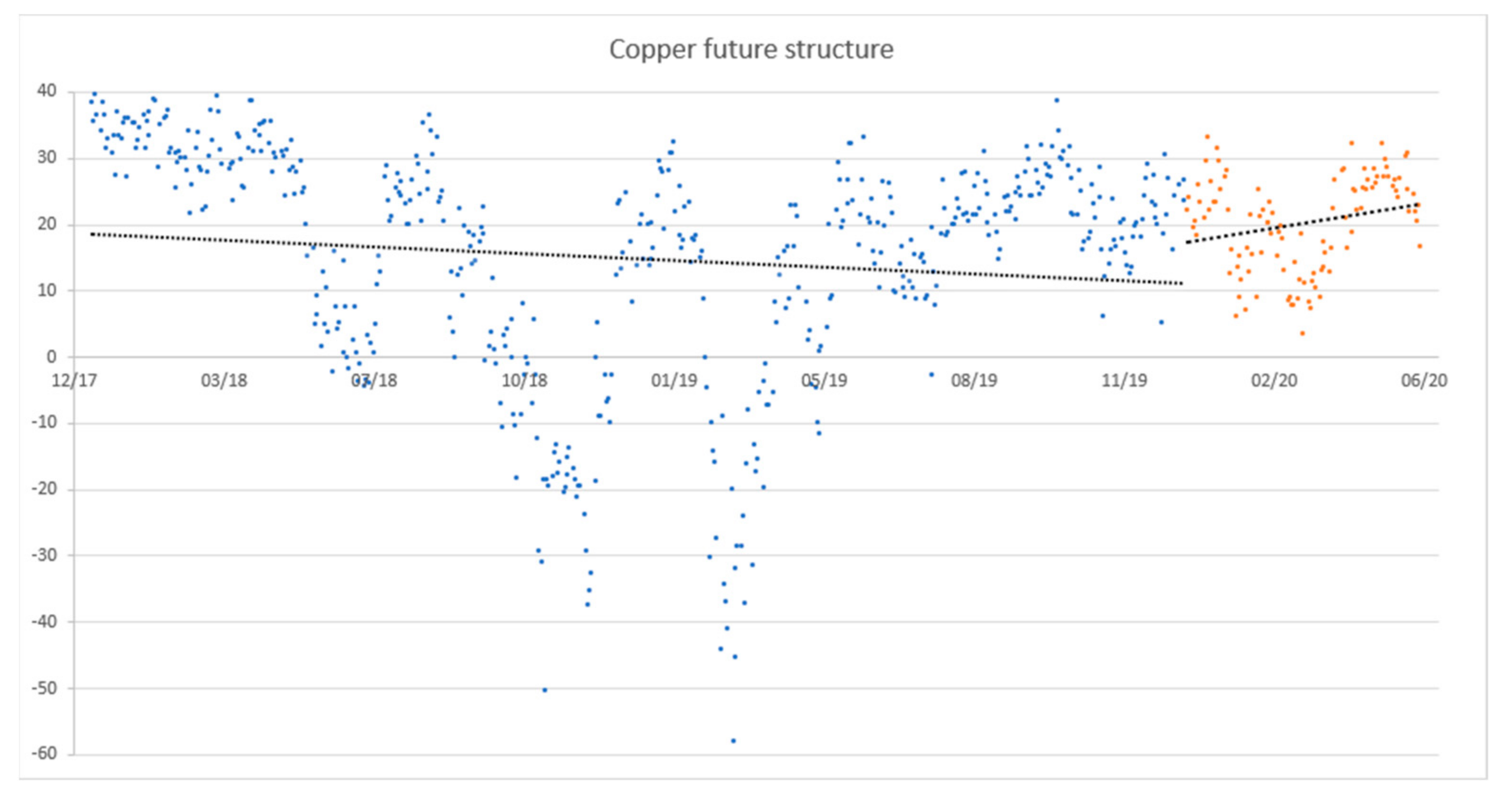
A better illustration of how COVID-19 has shocked the copper market in particular is offered by the descriptive change in tendency in the first half of 2020 (during the first wave of COVID-19 contagions in Europe) (see Figure 2). The figure shows LME copper market evolution, in reference to its official historical price structure, and it can be seen, too, how the market had been in a negative (−0.0102) trend, then in a positive one (+0.0362), in both cases, using a linear regression approach.

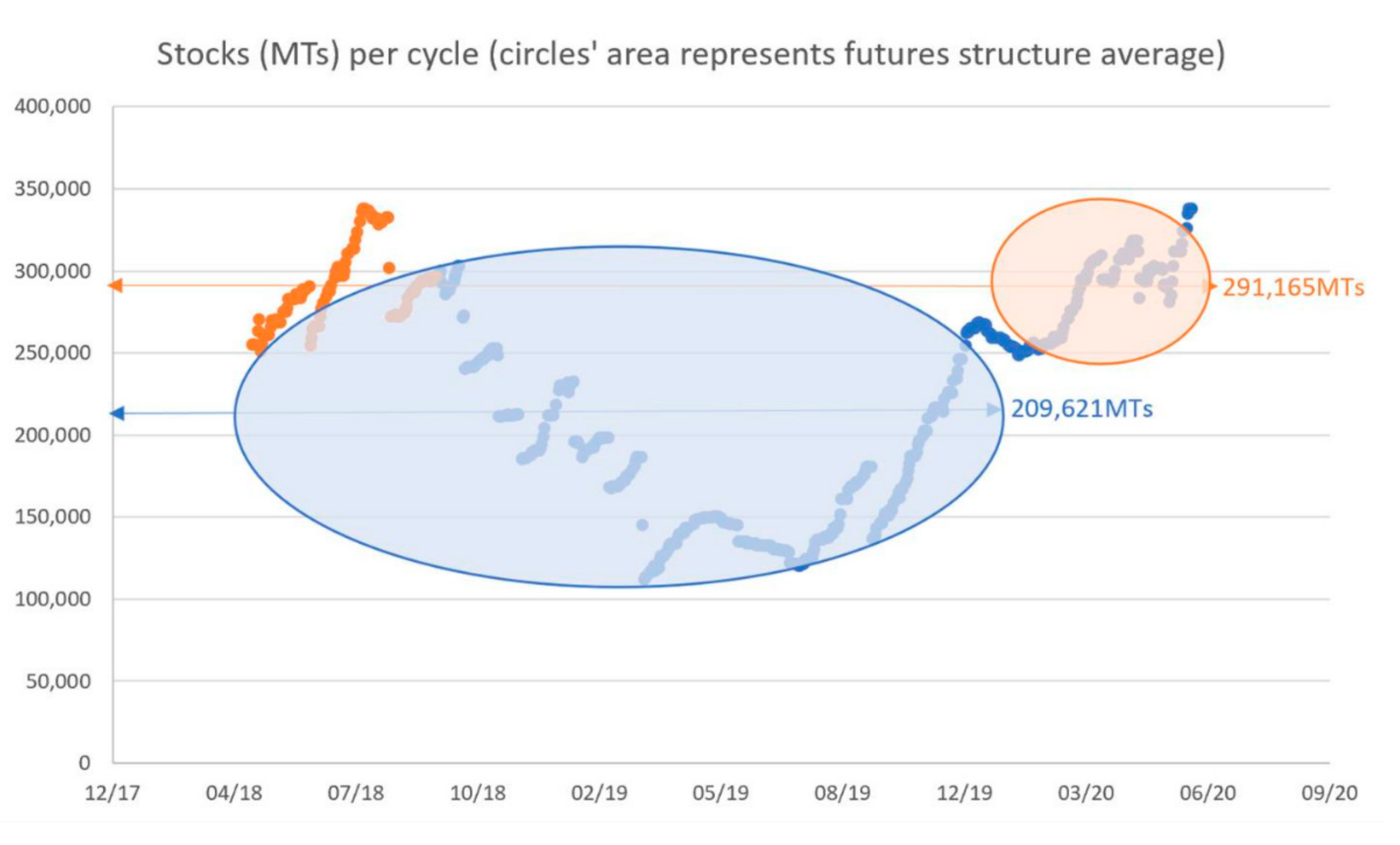
An additional illustration of the influence of the situation on stocks in the first half of 2020 is given by Figure 3, representing the average levels of stocks in warehouses.

Copper stocks significantly changed, as volume went from 209,621 MTs, on average, during 2018–2019, to 291,165 MTs, on average, during the first half of 2020, which represents a 39% increase.

The remainder of this paper is organized as follows. Section 2 reviews the relevant literature on cointegration, co-movements, copper, and the COVID-19 crisis. The data and methodology are reviewed in Section 3. A description of the results and an analytical review are presented in Section 4. Finally, conclusions and recommendations are discussed in Section 5.

2. Literature Review

The main aim of this study is to prove the appearance of “normal backwardation” under the conditions of a critical event, such as the COVID-19 pandemic. For this purpose, we have assessed the literature on co-movements and the COVID-19 pandemic.

2.1. Cointegration and Co-Movements: Copper

The influence of different variables on time series fluctuations has been a matter of global study within several economic environments and, specifically, in commodity markets, as has been assessed by [34,35] and, more recently, [36,37,38,39].

Some commodities’ prices move together, which is referred to as co-movement, such as in the energy markets [40,41] and oil markets [42], and between different metals [43,44,45,46] and in metal exchanges [47].

Interest in cointegration and causality has also been present in topics such as cryptocurrencies [48] and Brexit [49].

Copper has been chosen for this study for many reasons. First, it is one of the most financialized base metals priced on the Shanghai Futures Exchange (SHFE), the London Metal Exchange (LME), and the New York Commodity Exchange (COMEX), which are commonly used for speculative strategies [50]. Second, it has a large influence at different economic levels, for example in rich economies, such as Chile’s, and in the development of many others [51]. Third, it is one of the metals that are taking over the incipient metal super-cycle, due to the increase in needs and consumption related to the appearance of electric vehicles [52], the increase in renewable energies, and the use of electric applications in general. Given all these factors, authors such as [53] have identified a high probability of a lack of copper in the short term. This battle between the influence of fundamentals and financialization on copper markets has also been studied by [54]. In addition, cointegration and co-movements in the copper market have been a matter of study for authors such as [55], assessing not only copper but also another 43 commodities; [56], assessing efficiency in the structure of prices; [57], studying the cointegration of copper prices with China’s activity and stock returns, and finally [58], looking at cointegration in certain time periods between future prices and cash prices.

2.2. COVID-19 Influence on Markets

COVID-19 has been the biggest macroeconomic influence in recent history, affecting the global economy, the flow of trade, and human beings in general. Although this is a relatively recent matter, the numbers of studies and authors that have concentrated their efforts on investigating and rationalizing each step of this process has been extremely important. The economic effect of COVID-19 is obvious, as Appendix A shows.

Table 1. Articles concerning COVID-19’s influence on the commodities market.

Doc.	Topic/Theme	Context	Purpose	Key Findings
[59]	Co-movements in energy counterparties’ parameters under extreme conditions	COVID-19 crisis and West Texas Intermediate (WTI) oil future prices showing negative prices	To study transmissions and contagion in the energy sector	Existence of spillovers and co-movements among these energy-focused corporations
[60]	Connectedness in energy commodities after COVID-19 pandemic beginning	First two months of the COVID-19 outbreak	To look into the financial impact on COVID-19, concentrated on the energy sector	Dependence among energy commodities increases
[1]	Effect of the pandemic on the connectedness amongst the commodities market	US and worldwide COVID-19 pandemic effect	To explore the risk transmission in commodity and financial markets during the COVID-19 pandemic	Volatility connectedness between commodities and financial markets
[61]	Commodity price returns during the pandemic	COVID-19 Global Fear Index (GFI) rising	To examine how GFI is linked to commodity price returns	Commodity prices’ linkage with global COVID-19 fear index
[62]	Alternative markets study	COVID-19 beginning up to March 2020 and the safe haven assets	To study the effectiveness of safe haven markets under the COVID-19 crisis	The safe havens of gold and soybean
[63]	Study of some commodities’ market volatilities	Price prediction model changes during the COVID-19 crisis	To readapt the existing price prediction models to the variations caused by COVID-19	Volatility of commodity prices
[32]	Speculation on commodities	No speculation increase caused by other critical financial effects	To evidence the increase in the speculation of commodities (energy, soft and precious metals) in the presence of COVID-19 effects	Different influences on soft and hard commodities
[64]	Overreactions in commodities prices	Intraday price changes (changes of prices followed by proportional price reversals)	To identify how 20 different commodities react to COVID-19 effect on intraday prices	Commodity price overreactions in this period
[65]	Volatility connectedness among assets peaked during the outbreak	US ETFs, before COVID-19 and during the first wave (up to 29 May 2020)	Changes in the structure and time-varying patterns of volatility connectivity between stocks and major commodities (oil, gold, silver, and natural gas)	Volatility connectedness peaked during the COVID-19 pandemic
[66]	The influence of the COVID-19 pandemic on commodity prices	International commodity (metal and agricultural) prices (2 December 2019–1 October 2020)	To show, in the context of the COVID-19 pandemic, the impacts of oil supply and global demand shocks on metal and agricultural commodity prices	The pandemic represents a mix of supply, demand, and uncertainty shocks, and the result is that price indices have significantly declined as it continues to disrupt global supply and demand chains
[67]	Comparative commodity (oil and metals) prices	The COVID-19 outbreak generated price declines in precious and industrial metals, although drops were lower than in oil prices	To comprehensively address the potential impacts of the COVID-19 outbreak on commodity markets	Drop in oil market prices and metal prices, particularly in copper
[17]	Since the correlations between stocks, bonds, and commodity futures returns are likely to change over time, the weight of commodity futures in optimal portfolios could also be time-varying	Commodity futures have traditionally shown low correlations with stocks and bonds	Normal backwardation in commodity markets no longer works	End of normal backwardation in recent times and the difficulty of hedging in the present scenario
[31]	Trend-following strategies create significant abnormal returns in futures markets	A paired trading market–neutral strategy is used (through machine learning algorithms), involving long and short positions in two different future contracts with similar time series price trends	To show that normal backwardation and contango do not consistently characterize futures markets, but each futures market exhibits unique prevailing price trends	Algorithm of trading pairs in futures price structures and the effect on hedging strategies during the COVID-19 crisis

shows a compendium of articles showing COVID-19′s influences on the commodities market.

Therefore, the effects of co-movements on commodities in general and on copper in particular have been studied in depth in the literature. Finding are, in general, there is a dependence between the behaviors of the prices of these commodities and different factors, such as microeconomic and macroeconomic events. In this regard, COVID-19 is the recent event that has most strongly affected the whole structure of exchange markets, shaking the entire market’s structure in different sectors.

3. Data and Methodology

3.1. Data

The copper price data were obtained from the London Metal Exchange and have been used to establish the price structure upon official daily close of the market. The database includes 102 official LME calendar trading days, stretching between 13 January 2020 (day 44 of the pandemic, following [68], with the first case identified in China) and 5 June 2020 (day 188, when the first wave in Europe was considered under control), as used for a descriptive analysis of the first wave of contagions in Europe as the growth rate moved to zero (this interval has also been used by some other authors [69]). The COVID-19 data index we used was composed of the accumulated deaths collected each week in different regions of the world, according to the data published by the WHO, evaluating the number of cumulative deaths (weekly summarized) per population (10,000 habitants’ ratio) as per the United Nations World Populations Prospects 2019. These COVID-19 data were segmented by Date/Country/WHO_region/New_cases/Cumulative_cases/New_deaths/Cumulative deaths, and the different regions are shown in

Table 2. Regions as per WHO.

European Region	EURO
Eastern Mediterranean Region	EMRO
Western Pacific Region	WPRO
African Region	AFRO
Region of the Americas	PAHO
South-East Asia Region	SEARO

below.

3.1.1. WHO Weekly Mortality Index

We have used the percentage of increase in cumulative deaths, measured weekly as a percentage per 100,000 habitants, as cases detected during the first wave were not measured in the same diametric manner in every country (due to the different capacities to do so) and weekend data were usually not published on time by every country. The availability of tests and the differences in how countries report their figures have been amongst the biggest limitations to our data.

The figures show the data on the biggest countries in each WHO region to perform a descriptive analysis of the information available.

The COVID-19 weekly mortality index (represented by the time series COVIDt) was obtained through arithmetic assessments of the data given every Monday by WHO, focusing on the difference in cumulative deaths between one reference and that from the previous week. The percentage of growth shown by one reference over this period is the focus of our study. These data have been assessed for the number of inhabitants in every region. As such, we can establish:

Day 1 Cumulative deaths 1 Mortality assessed 1

Day 8 Cumulative deaths 2 Mortality assessed 2

INDEX = (Cumulative deaths 2 − Cumulative deaths 1) ∗ 100/Number of inhabitants

(1)

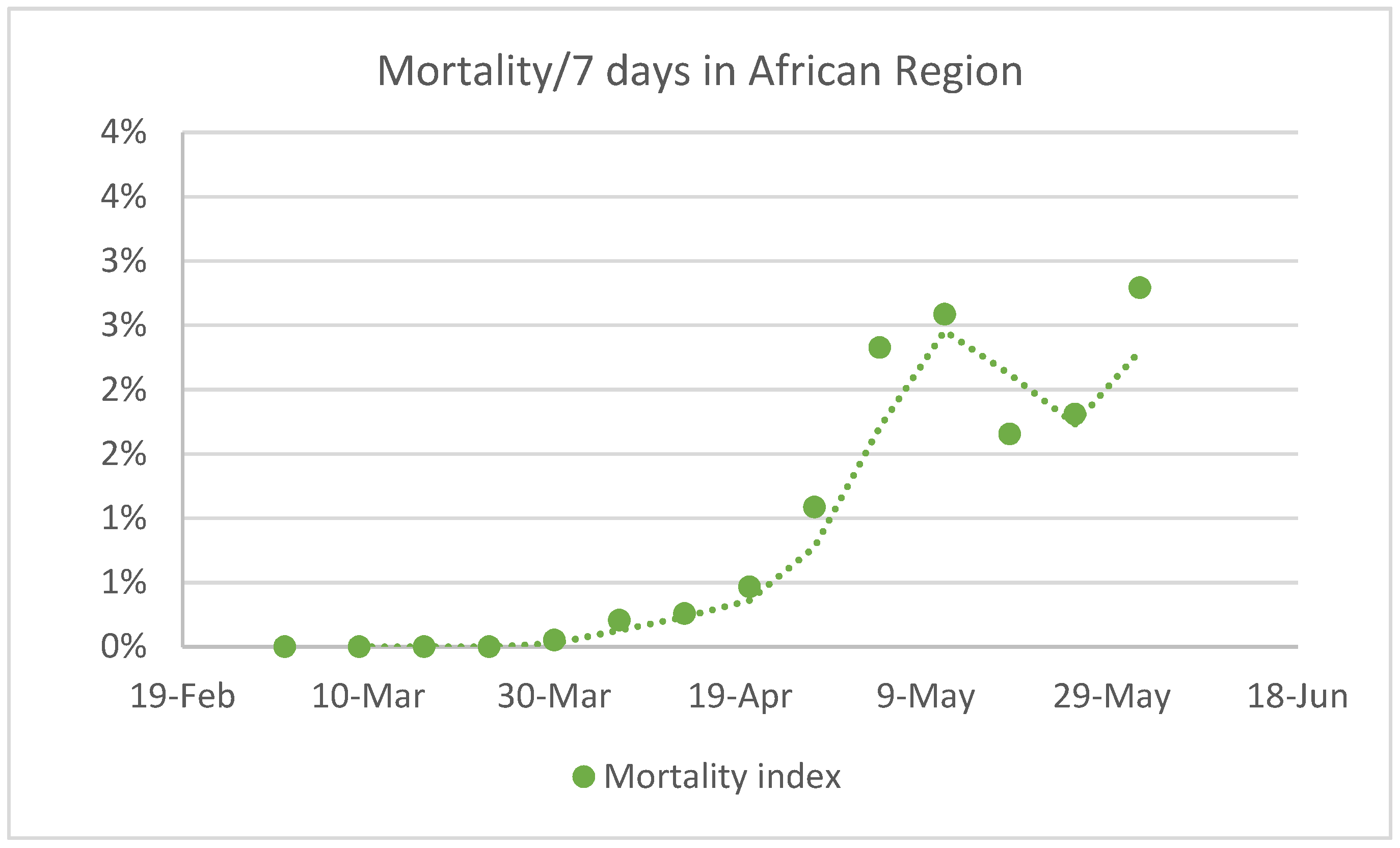
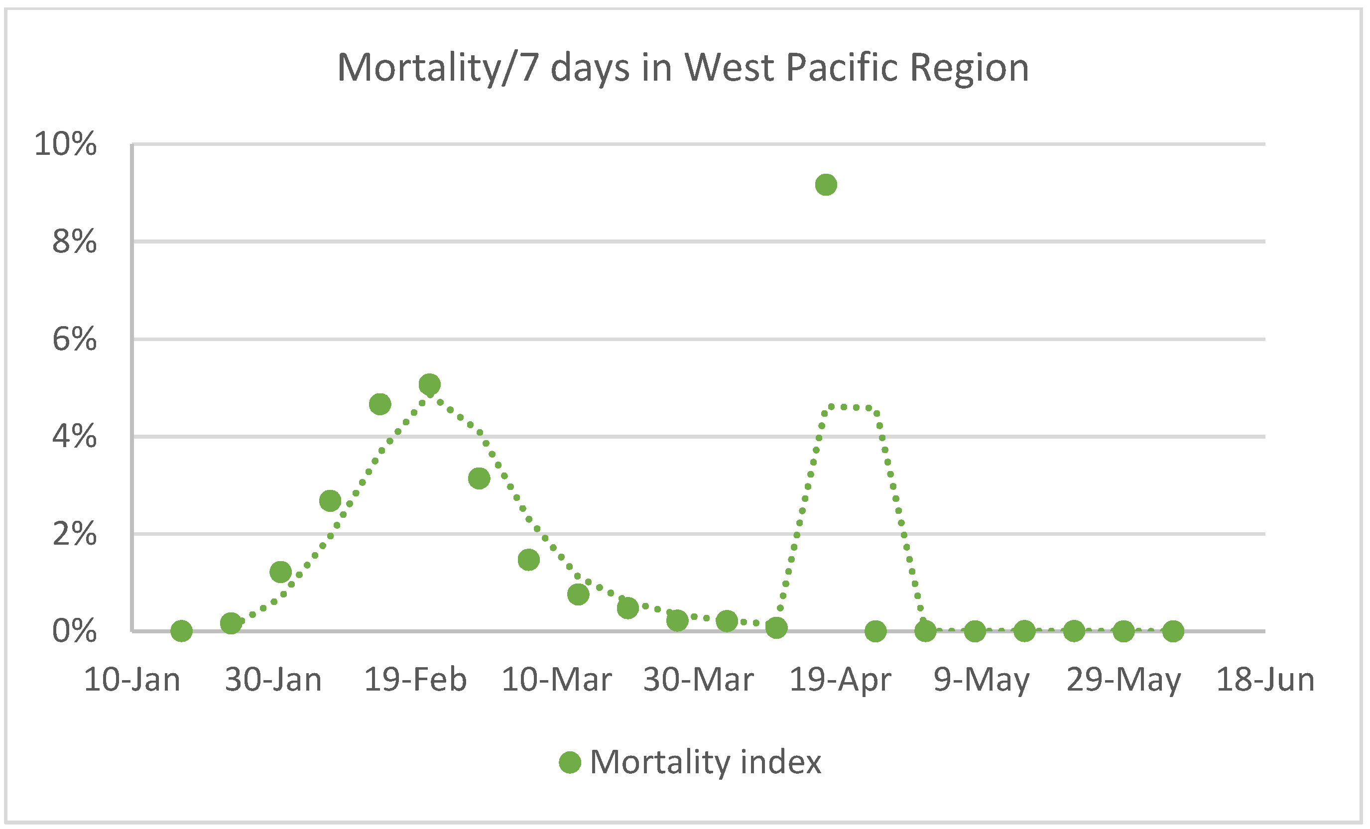
Cumulative deaths data from Monday to Sunday were calculated through the sum of daily deaths that were published. Even though Europe alone is the subject of our investigation, we display the results for the six areas (see Figure 4, Figure 5, Figure 6, Figure 7, Figure 8 and Figure 9).

Low values were found in African and West Pacific regions during the first wave of contagions in Europe, and these are mainly related to the low ages of the populations in the main countries in the African area and to the heavy measures taken to control the pandemic in the West Pacific region.

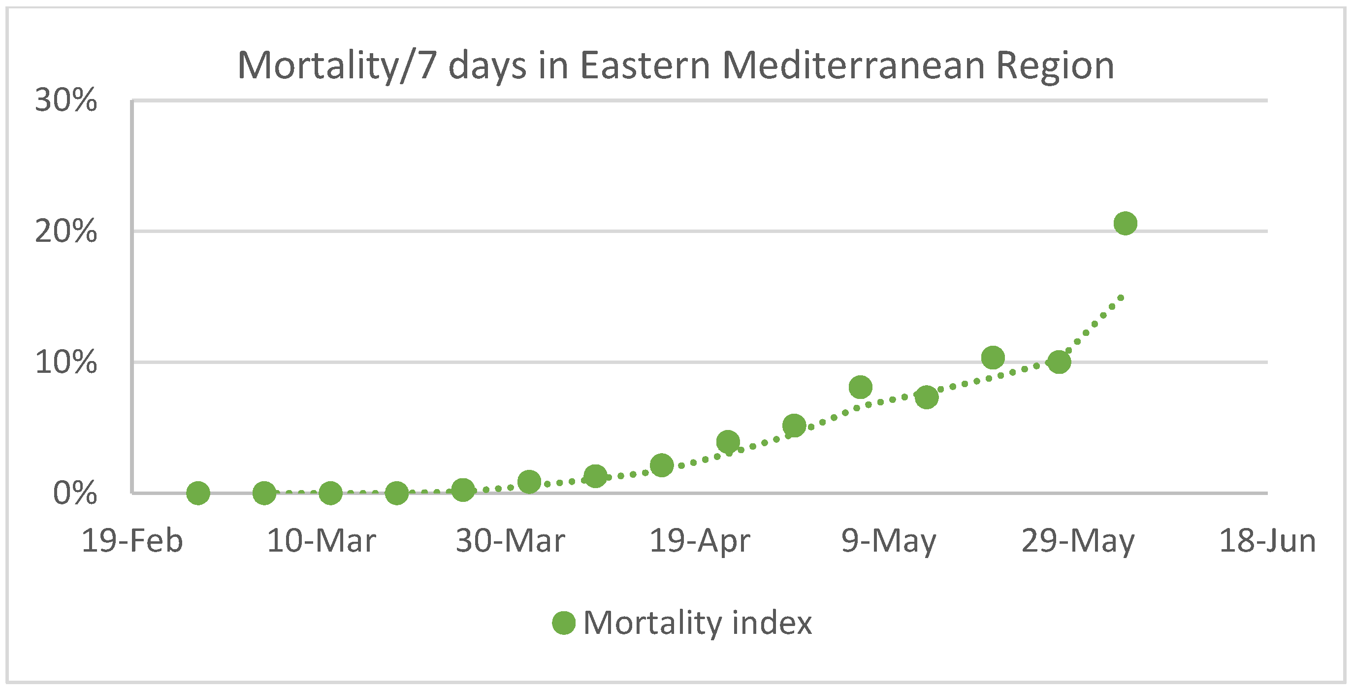
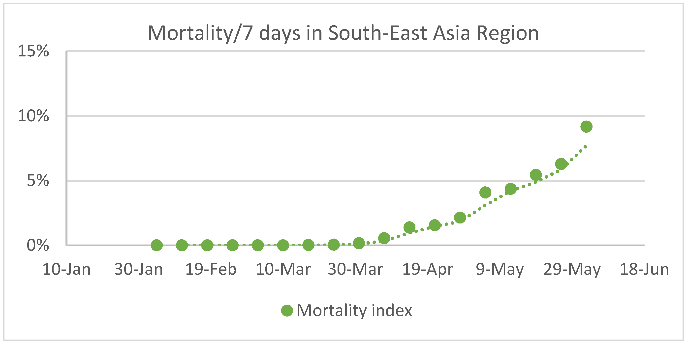
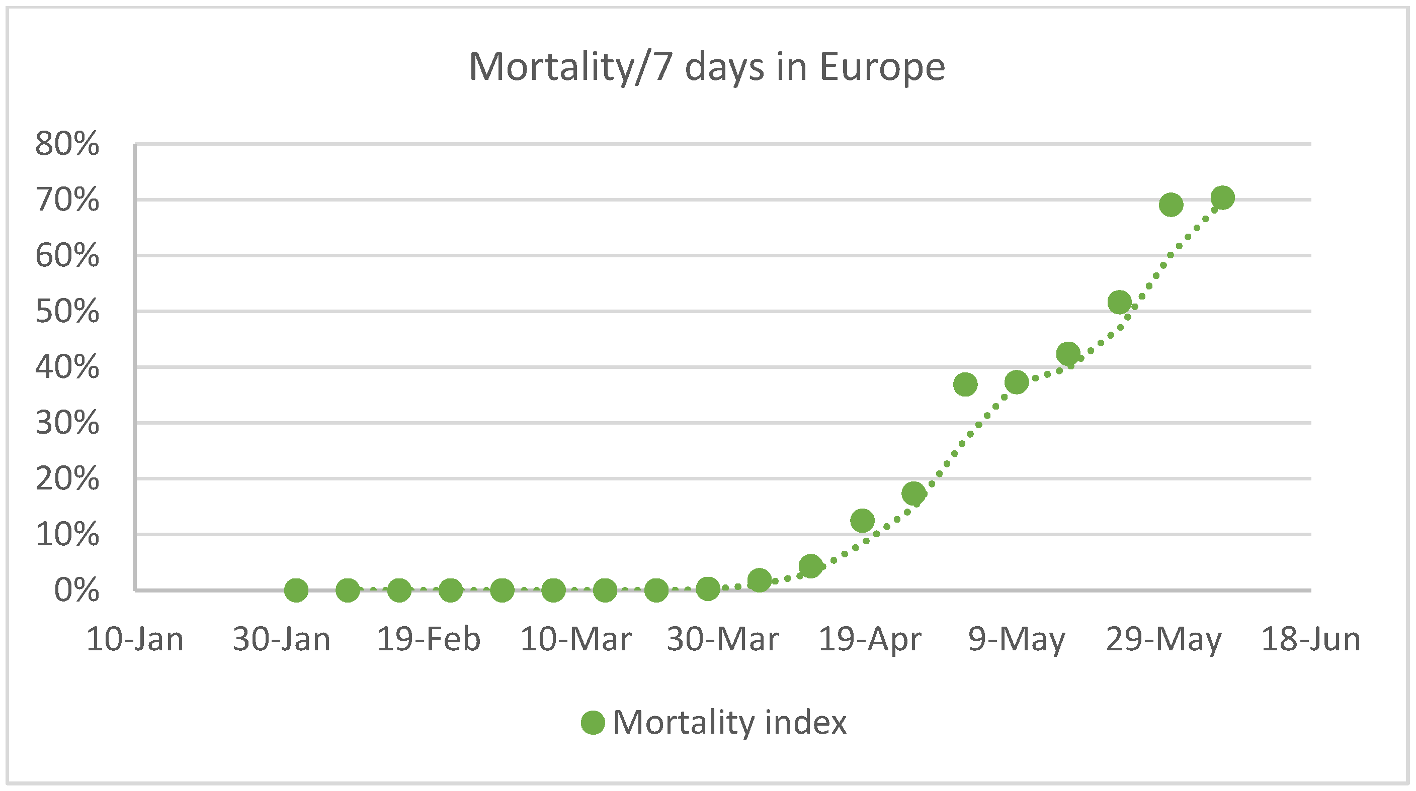
Eastern Mediterranean, South-Eats Asia and Europe regions have shown constant increases, but Europe has shown a very significant constant increase in the seven days mortality index.

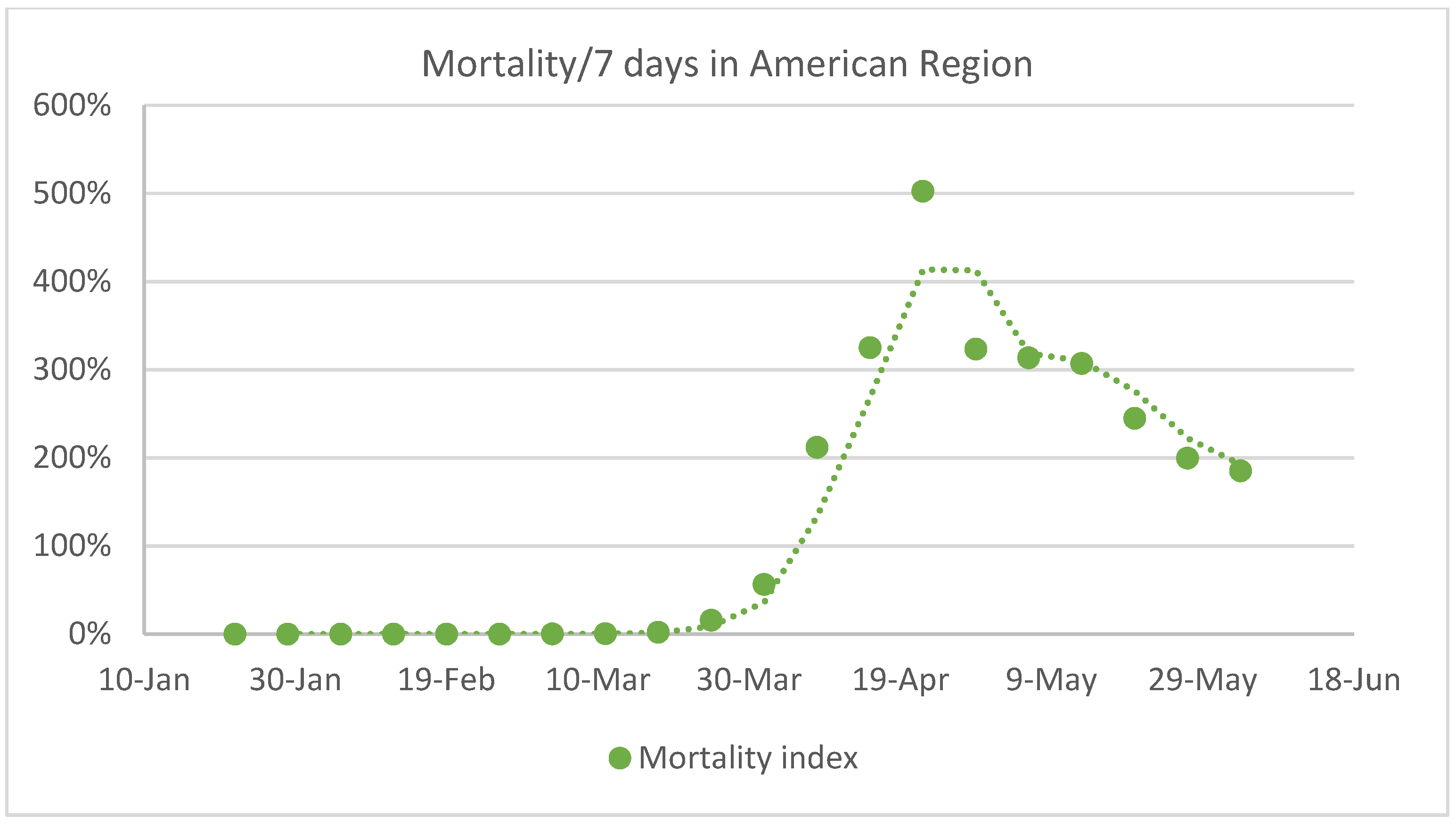
The American region has shown a constantly increasing ratio indicating an uncontrolled pandemic situation followed by a period of apparent control, with a substantial drop in the percentage of increase in deaths due to COVID-19; the reality, however, is that the increase was so big (achieving values of more than 500%) that the decrease appears as 200%.

3.1.2. LME Data: Prices and Warehouses’ Stocks

The allocation of the futures price structure is derived from the difference between the 3-month control reference and the cash or spot price. The 3-month basis is a liquid position [70] and is that to which the whole market refers a large part of its operations; therefore, this metal’s structure refers to this difference, whereby a positive difference indicates contango and a negative one indicates backwardation.

The most common market structure should be contango, as the warehousing system is a regulator. Backwardation should only arise in a forced market, related to a lack of offer, an excess of demand, or a speculative global fund trading position. Nevertheless, this situation is becoming more and more frequent, with long periods of backwardation arising due to the developing super-cycle of metals [71,72].

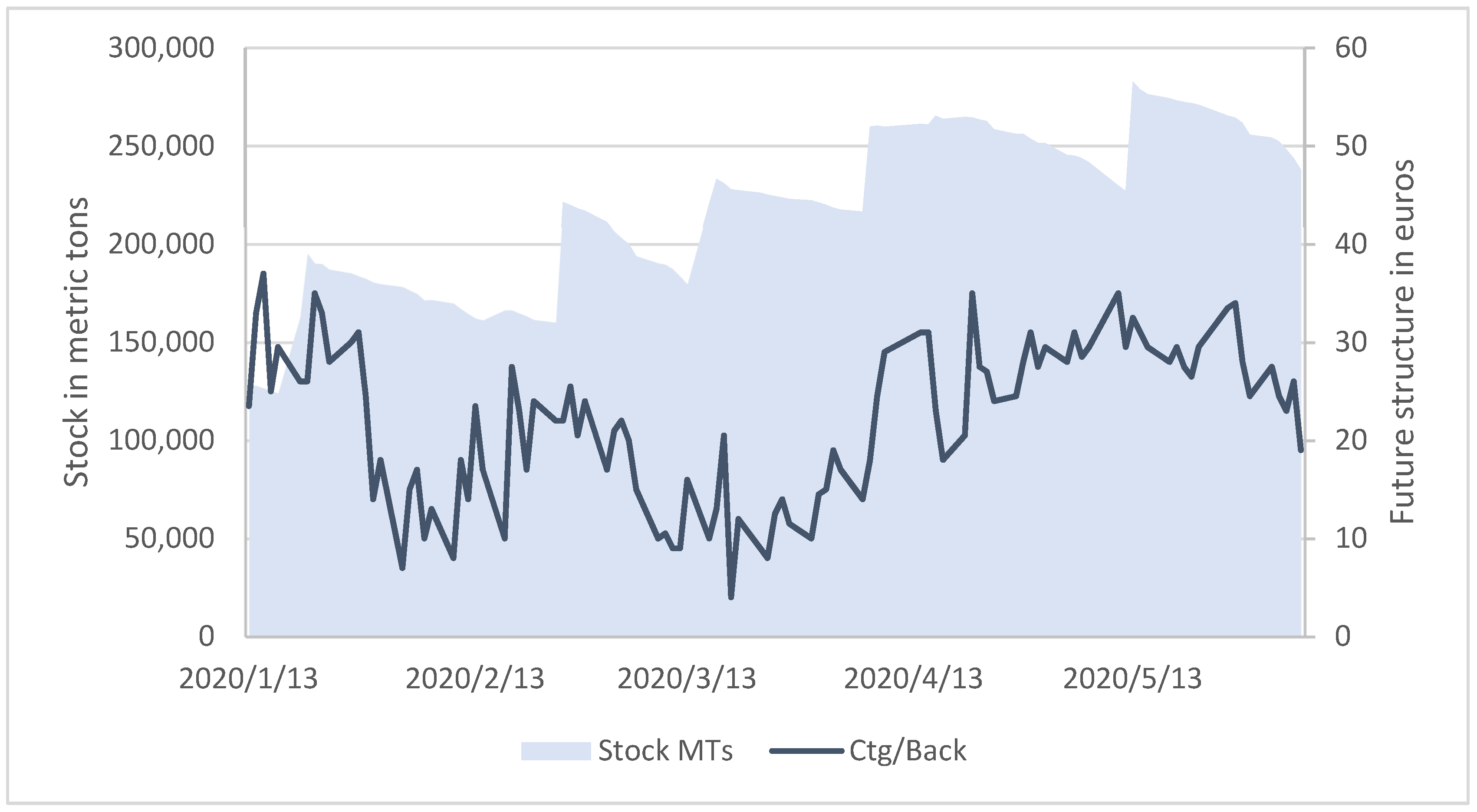
The copper futures price structure data were taken from the LME and warehouses stock for the same period; the LME uses a worldwide warehouse system to normalize different levels of metal demand and offers. Producers and traders can place large amounts of metal into these warehouses if its brand and quality are assured by the LME’s standards; this can be done through brokers, who also need to be listed under the LME’s standards. As the premium for introducing a metal into an LME warehouse is null, producers prefer to sell directly to the market so as to achieve a premium; therefore, it is usually only when the direct consumer market is not active or is sparse that metals arrive at these warehouses. Traders can also perform this type of operation to manipulate the structure of the prices or the forward curve in favor of their short- or long-term global positions. The levels of copper in LME’s warehouses and the structure of the copper futures prices are shown in Figure 10.

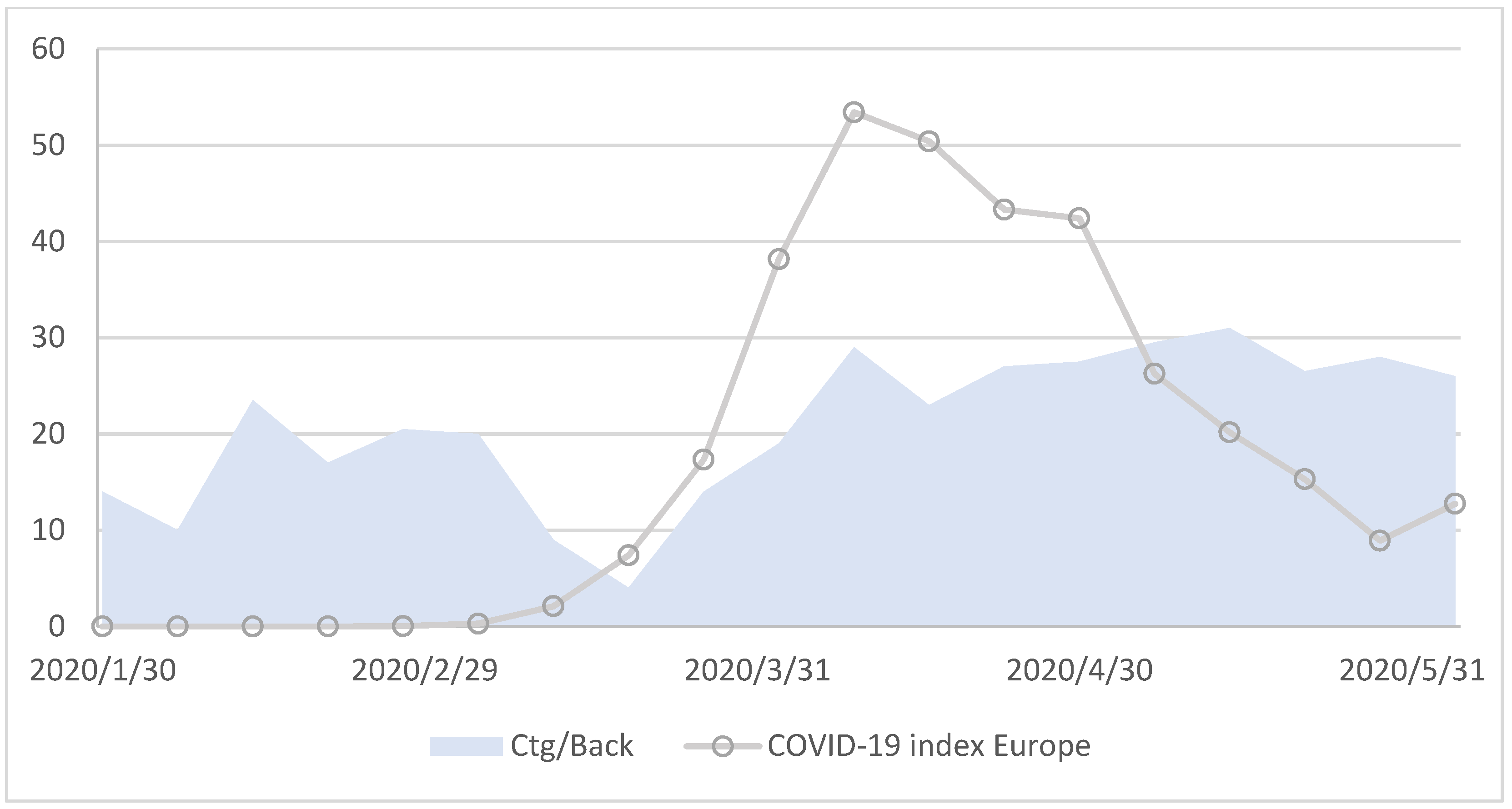
European data were chosen for this analysis for three reasons. First, Europe is one of the major economies outside of China; second, it is where the LME warehouses have been established; third, its markets are mostly based on fundamentals. Additionally, descriptive analysis also supports the strategy of using Europe as the basis of this study, as the same trends are shown in their COVID-19 indexes as in the changes in LME warehouses.

Both data series—the COVID-19 index in Europe and the LME copper futures price structure—are represented in Figure 11.

3.2. Methodology

Unit root tests have been performed to ensure that the time series do not follow a random walk structure, ensuring that they are stationary and that causality tests can be used. In this regard, our aim was to identify the situation wherein series bind together, with no deviation from equilibrium in the long run.

In these types of unit root tests, the null hypothesis can be linked with the stationarity of the time series, as in the ADF and PP tests, as well as in different ones, such as KPSS tests.

Because the time series addressed in this study were non-stationary and exhibited non-constant variance, they were analyzed with the augmented Dickey–Fuller (ADF) [27] unit root test, as recently deployed by [73] and [74].

The three regression models for ADF are set out below:

$$\Delta y_t={\psi }_{ADF}{y}_{t-1}+{{\displaystyle \sum }}_{i=1}^{p-1}{\psi }_i\Delta y_{t-1}+u_t; u_t\approx IID\left(0,{\sigma }^2\right); t=1, 2, \dots ,$$

(2)

$$\Delta y_t={\psi }_{ADF}{y}_{t-1}+{{\displaystyle \sum }}_{i=1}^{p-1}{\psi }_i\Delta y_{t-1}+\mu +u_t; u_t\approx IID\left(0,{\sigma }^2\right); t=1, 2, \dots ,$$

(3)

$$\Delta y_t={\psi }_{ADF}{y}_{t-1}+{\displaystyle \sum }_{i=1}^{p-1}{\psi }_i\Delta y_{t-1}+\mu +\mathsf{\gamma }\mathrm{t}+u_t; u_t\approx IID\left(0,{\sigma }^2\right); t=1, 2, \dots ,$$

(4)

In these equations, the difference between two time values is a function of non-constant variance u_t, with or without constant drift, µ, and a trend term, γ_t.

The symbols in the above expressions are defined below.

Ψ_ADF, parameter determining the fulfilment or otherwise of the null hypothesis.

${{\displaystyle \sum }}_{i=1}^{p-1}{\psi }_i\Delta y_{t-1}$, sum of differentials in the value series multiplied by Ψ in p − 1 iterations.

p, maximum regression delay.

µ, constant.

γ_t, trend.

u_t, process error, a function of the variance series.

The ADF and Phillips–Perron test that there is a unit root for a times series as a null hypothesis. The existence of a unit root implies that the process is non-stationary. KPSS tests the null hypothesis that there is stationarity in the series [75].

Engle and Granger causality-based cointegration tests [33] were performed on the transformed series. The latter yield the order of autoregressive vectors (VAR) [76] and a basis for calculating λ_max using Johansen’s approximation, which is used to find at least one cointegration relationship between the two series.

The Granger causality theory (Johansen approximation [30]) was used to analyze the relationship between the series ${(y_t)}_{t=1}^N$.

$$\mathrm{Structure}\mathrm{of}\mathrm{copper}\mathrm{futures}\mathrm{prices},{(y_t)}_{t=1}^N:{(str{u}_t)}_{t=05-06-2020}^{13-01-2020}$$

(5)

$$\mathrm{Stocks}\mathrm{in}\mathrm{warehouses},{(z_t)}_{t=1}^N:{(STOC{K}_t)}_{t=05-06-2020}^{13-01-2020}$$

(6)

On the other hand,

$$\mathrm{Structure}\mathrm{of}\mathrm{copper}\mathrm{futures}\mathrm{prices},{(y_t)}_{t=1}^N:{(str{u}_t)}_{t=05-06-2020}^{13-01-2020}$$

(7)

$$\mathrm{COVID}-19\mathrm{weekly}\mathrm{deaths}\mathrm{index},{(z_t)}_{t=1}^N:{(COVI{D}_t)}_{t=05-06-2020}^{13-01-2020}$$

(8)

To resolve the equations shown below ((9)–(12)), Engle and Granger cointegration tests were conducted by applying ordinary Least Squares (OLS) to the transformed data series:

On the one hand,

$$str{u}_{t }={\alpha }_0+{\alpha }_1 str{u}_{t-1}+\dots +{\alpha }_1 str{u}_{t-d}+{\beta }_1 str{u}_{t-1}+\dots +{\beta }_1 stoc{k}_{t-d}+{\epsilon }_t$$

(9)

$$stoc{k}_{t }={\alpha }_0+{\alpha }_1 stoc{k}_{t-1}+\dots +{\alpha }_1 stoc{k}_{t-d}+{\beta }_1 stoc{k}_{t-1}+\dots +{\beta }_1 str{u}_{t-d}+u_t$$

(10)

where d is the number of delays used, $str{u}_{t}and$$stoc{k}_t$are the time series for which cointegration was to be determined, α and β are the parameters to be studied, and ε_t and u_t are the errors or random disturbance, which are normally uncorrelated. It is necessary to fit a vector autoregressive (VAR) model to obtain the optimum lag model [76].

On the other hand,

$$str{u}_{t }={\alpha }_0+{\alpha }_1 str{u}_{t-1}+\dots +{\alpha }_1 str{u}_{t-d}+{\beta }_1 str{u}_{t-1}+\dots +{\beta }_1 COVI{D}_{t-d}+{\epsilon }_t$$

(11)

$$COVI{D}_{t }={\alpha }_0+{\alpha }_1 COVI{D}_{t-1}+\dots +{\alpha }_1 COVI{D}_{t-d}+{\beta }_1 COVI{D}_{t-1}+\dots +{\beta }_1 str{u}_{t-d}+u_t$$

(12)

for the other pair of data series studied.

Finally, a robustness test was done, studying cointegration between the independent variables of the above analysis: COVIDt and STOCK_t.

From a methodological point of view, once the series are transformed enough times to obtain stationarity, these series can be represented as a set of p iterations with consecutive values, as follows:

$$y_{t }=c+A_1 y_{t-1}+A_2 y_{t-2}+\dots ++A_p y_{t-p}+e_t$$

(13)

in which the values are corrected by a series of constants, such as A_i, where i = 1, …, n; the input constant is c, and the error vector is e_t.

The p-value of Equation (13) defines the VAR order of the series [77]. Here, it was found with the Schwarz or Bayesian (BIC) and Akaike information criteria (AIC), as defined by [78]:

$$\mathrm{Akaike}\left(\mathrm{AIC}\right):AIC\equiv -\frac{2L^{*}}{n}+\frac{2m}{n}$$

(14)

$$\mathrm{Schwarz}\mathrm{or}\mathrm{Bayesian}\left(\mathrm{BIC}\right):BIC\equiv -\frac{2L^{*}}{n}+\frac{m ln\left(n\right)}{n}$$

(15)

where L* is the Napierian logarithm of the likelihood function; n is the number of observations, and m is the number of estimated parameters.

The Johansen approximation yields α and β as the vectors:

α = |p,r| and β = |m,r|

(16)

where r is the number of cointegrating vectors, and p and m are the series vector components.

The premise underlying the maximum lambda and trace tests was described by [79] as follows: “The maximum likelihood theory of systems of potentially cointegrated stochastic variables presupposes that the variables are integrated of order 1, or I(1), and that the data-generating process is a Gaussian vector autoregressive model of finite order l, or VAR(l), possibly including some determinant components”. The trace test is defined in the following terms:

$$Trace=-T {{\displaystyle \sum }}_{i=r+1}^p\log (1-{\lambda }_i)$$

(17)

where λ_i are the eigenvalues in ascending order that deliver the solution to the “reduced rank regression problem”, and r and p form parts of values α and β, as above.

The test is run consecutively for r values of r = p − 1, …, 0 or r = 0, …, p − 1, up to the value at which the null hypothesis is first rejected, or to the end of the series if it is not rejected.

Instead of r, the validity of the null hypothesis may also be determined from r + 1, which constitutes the λ_max test, which is the one used here:

$${\lambda }_{max}=-T\log \left(1-{\lambda }_{r+1}\right)$$

(18)

which is identical to the trace test when p − r = 1.

Finally, it is necessary to determine whether one variable “Granger-causes” another. One variable causes the other if the past values of one are useful for predicting the other. See Appendix B for an extensive explanation of the application of this methodology in different markets.

The residuals of the linear regressions built from the different data series are a matter of study in this paper, as assessed through the Durbin–Watson approach [80,81,82].

Under this theory, the errors complete the definition of each time series, defined as ε_t, and taking in this formula, the definition of the statistic D can be given as

$$D=\frac{{{\displaystyle \sum }}_{t=2}^n{({\mathsf{\epsilon }}_t-{\mathsf{\epsilon }}_{t-1})}^2}{{{\displaystyle \sum }}_{t=1}^n{\mathsf{\epsilon }}_t{}^2}$$

where t refers to the different observations of the time series.

The null and alternative hypotheses of this test are H0, where the errors are not correlated, and H1, where they are. With a p-value below the significance level, we can certify that the residuals are sufficient to use in the following tests on the time series.

4. Results

In this section, we give the relations between the structure of copper futures, the LME copper warehouses’ level, and the COVID-19 weekly mortality index during the first wave of contagions in Europe. We have also seen, in general, how extreme events are linked with big effects on the future price in comparison with the cash price, ultimately developing a contango structure, evidencing the theoretical background of so-called “normal backwardation”.

4.1. Relationship between LME Copper Warehouses’ Level and the Structure of Copper Futures Prices

Both series STOCK_t and stru_t have been shown to be non-stationary, even after Box–Cox [83] transformations, and we also found non-stationarity at the following levels of both series. We confirmed this via ADF, PP, and KPSS tests to check the non-stationary of the two series, STOCK_t and stru_t, as can be seen in

Table 3. Stationary tests for STOCK_t and stru_t.

	p-Value
Data Series		ADF	PP	KPSS
Stock MTs	I(0)	0.893	0.893	<0.0001
strut	I(0)	0.177	0.177	0.008
Stock MTs	I(1)	0.833	0.435	<0.0001
strut	I(1)	0.218	0.218	0.004

, finding that both series are non-stationary to the same degree. In regard to causality, Johansen’s approximation of the cointegration test of Engel and Granger was performed (see

Table 4. Johansen’s approximation tests for causality STOCK_t and stru_t.

p-Value
Data Series	Lambda Max	Trace Test	VAR Estimation (AIC)
Stock MTs	0.048 **	0.072 *	2 (21,988)
strut

** Rejection of the null hypothesis at the 5% significance level. * Rejection of the null hypothesis at the 10% significance level.

), obtaining cointegration between the STOCK_t and stru_t series in the time frame studied. This means that increases in contango and stocks are linked, giving evidence for the theory of normal backwardation.

This means that, under strongly adverse conditions in the consumption market, because of economic crises, sanitary catastrophes, low demand, or other extreme events, economic players, such as producers or traders, are forced to allocate their units to official warehouses instead of to final consumption markets. From a practical point of view, this means that copper producers cannot easily alter their volumes to adapt to rapid decreases in market consumption. This is also a characteristic of the commodity market, wherein a complex global system of warehouses is established specifically “to regulate the inflows with the outflows”. The specific definition of backwardation based on fundamentals refers to the lack of availability of metal on the market, and in general, to the feeling of scarcity; therefore, contango means the opposite, that is, the excess of availability. Our findings definitely support this fundamentals-based definition of contango, as under the conditions of a sanitary crisis, with a lack of consumption and the same production model, market inflows are higher than outflows, with a strongly positive offer–demand balance, excess being allocated to the official warehouses.

This theory can be used by market players when establishing their positions in favor of contango when such market disruptions are about to occur.

4.2. Relationship between COVID-19 Mortality Index and the Structure of Copper Futures Prices

As in the previous assessment of the series, we have also checked the stationarity of stru_t, this being the futures copper price structure data series, finding (see

Table 5. Stationary tests for COVID-19 index and stru_t.

p-Value
Data Series		ADF	PP	KPSS
COVID-19 index	I(0)	0.459	0.459	0.048
strut	I(0)	0.177	0.177	0.008
COVID-19 index	I(1)	0.459	0.459	0.048
strut	I(1)	0.218	0.218	0.004

) that for both series (this one and the COVID-19 mortality data index), non-stationary conditions were achieved. After Box–Cox transformations, we also found non-stationarity in the following levels of both series.

Both data series, before and after being transformed, showed the same levels of non-stationarity, making it appropriate to use Johansen’s approximation of the Engel and Granger cointegration test to obtain co-movements between the COVID-19 index and the future price structure of copper (see

Table 6. Johansen’s approximation tests for causality COVID-19 index and stru_t.

p-Value
Data Series	Lambda Max	Trace Test	VAR Estimation (AIC)
COVID-19 index	0.003 ***	0.001 ***	5 (7.088)
strut

*** Rejection of the null hypothesis at the 1% significance level.

).

These results show that an event with a strong impact on demand (such as the increase in COVID-19 mortality rate) can cause market scarcity to disappear; in fact, it could generate a feeling of oversupply, thus developing a contango structure.

A producer that is starting to feel a lack of consumption interest from their customers due to a macro event, such as an incipient economic crisis or a sanitary emergency, could easily reassert their hedge position by selling their units using future due date prices instead of short-term prices. A good example of this has been the appearance of new variants of COVID-19, as a result of which the market could be preparing to restructure into a consistent contango. This approach, as others, is speculative by nature, so what is offered here is a better chance to prepare a strategy, as the market could have opposing drivers that would make the structures of copper futures prices fall into backwardation.

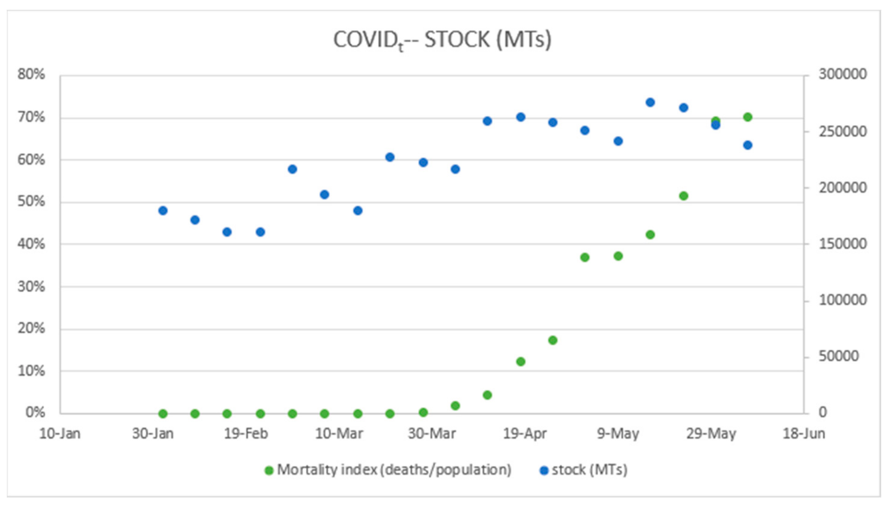
Relative to the joint evolution of COVIDt and LME warehouses stock series, as a robustness test, we have found that they are cointegrated. See Figure 12 and

Table 7. Engle and Granger through Johansen’s approximation values on cointegration.

p-Value
Data Series	Lambda Max	Trace Test	VAR Estimation (AIC)
COVIDt	0.011 **	0.006 ***	5 (13,645)
stock

*** Rejection of the null hypothesis at the 1% significance level. ** Rejection of the null hypothesis at the 5% significance level.

, showing p-values of Engle and Granger test:

Finally, we tested the null hypothesis that residuals of the model are autocorrelated. Time series’ residuals have been checked via the Durbin–Watson test, trying to certify that these residuals are autocorrelated and the tendency is consistent. The results show (see

Table 8. The p-value of Durbin–Watson tests performed on different time series.

Time Series	Warehouse Stocks	Structure of Daily Dataset	COVID-19 Index	Futures Price Structure on Weekly Dataset
p-value	<0.0001 ***	<0.0001 ***	0.029 ***	<0.0001 ***

*** Rejection of the null hypothesis at the 1% significance level.

) that, in the case of the series: warehouse stocks, structure of daily dataset, and futures price structure, the p-value is less than the 1% and, in the case of the COVID-19 series, the p-value is lower than the 5%, so the null hypothesis can be rejected.

5. Conclusions and Recommendations

The COVID-19 pandemic has thrown the world economy into turmoil, and commodity markets have lived through a tsunami since its beginning; its implications have led to a situation of strong normal backwardation.

This paper shows that the levels of stocks in warehouses are linked with the development of the commodity forward price (contango or backwardation). We proved that, in a multi-country lockdown scenario due to the first wave of COVID-19 infections in Europe, in a long-term backwardated context, copper stocks rose, and a contango structure appeared, indicating a cointegration between the data series representing these stocks and the contango structure.

In the same context, under the influence of macroeconomic events affecting commodity prices, the present findings confirm the existence of a relationship between COVID-19′s impact and the structure of copper futures prices, measured on the grounds of COVID-19 weekly mortality data.

In recent times, the financialization of commodities, especially copper, has been a matter of close study and investigation, as explored in the Introduction section, and we are finding that fundamentals are also interfering in the forward price compared with spot prices. Times are approaching where analyses and statistics are suggesting there will be a lack of copper units [52,53], so we can expect this commodity to be driven increasingly by fundamentals. The development of the EV (electric vehicle) and its higher level of copper usage for fabrication, the electrification of charging points, and the development of renewable energies are causing increases in optimism and a feeling that, again, fundamentals are playing an increasingly definitive role.

In this context, some highlights can be selected as policy recommendations, when market agents follow price structure strategies. Under normal backwardation theory, backwardation is the long-term trend; that implies that the spot price is higher than the 3-month price, so, depending on the position players have (short or long), they can try to move in favor of backwardation. However, an extreme event like COVID-19, that turned it into a contango, makes spot prices lower. This way, as contango appears, players should, then, set long term positions to optimize results.

Market players can benefit from changes in tendency and extreme events, such as the recent one studied here, related to the change from structural backwardation to contango. This fact can be used by volatility-based players to increase the weight of positions supported by extreme events, not only in terms of short-term contango or short-term backwardation, but also to set up a contango/backwardation structure change-based strategy. We have experienced, during the COVID-19 pandemic, different scenarios within the commodities market, showing the strongest contangos ever during the first phase of worldwide lockdowns, followed by several ups and downs in the future structure of base metals in particular, as related to extreme events (in our recent context, COVID-19): the arrival of a vaccine, the acceleration of the vaccination process, the appearance of new variants, countries’ herd immunity, new variants evading the protection of vaccines, new vaccines, new contagion waves, cross-relations between the variables under study, relations with other assets such as those in [69], etc. There is no doubt that the analysis of the commodities market’s behavior in general, and that of copper’s in particular, under all these scenarios opens up a new line of research and constitutes the basis of new papers. Additionally, the relation between data from the WHO regions and aggregated data from around the world could be a new research focus, even if it would be a huge challenge to measure the integrity of the data given the speed of communication between each country.

References

1. Adekoya, O.B.; Oliyide, J.A. How COVID-19 drives connectedness among commodity and financial markets: Evidence from TVP-VAR and causality-in-quantiles techniques. Resour. Policy 2021, 70, 101898. [Google Scholar] [CrossRef] [PubMed]
2. Ahmed, M.Y.; Sarkodie, S.A. COVID-19 pandemic and economic policy uncertainty regimes affect commodity market volatility. Resour. Policy 2021, 74, 102303. [Google Scholar] [CrossRef] [PubMed]
3. Lahiani, A.; Mefteh-Wali, S.; Vasbieva, D.G. The safe-haven property of precious metal commodities in the COVID-19 era. Resour. Policy 2021, 74, 102340. [Google Scholar] [CrossRef]
4. Ge, Y.; Tang, K. Commodity prices and GDP growth. Int. Rev. Financ. Anal. 2020, 71, 101512. [Google Scholar] [CrossRef]
5. Creti, A.; Joëts, M.; Mignon, V. On the links between stock and commodity markets’ volatility. Energy Econ. 2013, 37, 16–28. [Google Scholar] [CrossRef] [Green Version]
6. Liu, L.; Tan, S.; Wang, Y. Can commodity prices forecast exchange rates? Energy Econ. 2020, 87, 104719. [Google Scholar] [CrossRef]
7. Bouri, E.; Cepni, O.; Gabauer, D.; Gupta, R. Return connectedness across asset classes around the COVID-19 outbreak. Int. Rev. Financ. Anal. 2021, 73, 101646. [Google Scholar] [CrossRef]
8. Ji, Q.; Bouri, E.; Roubaud, D. Dynamic network of implied volatility transmission among US equities, strategic commodities, and BRICS equities. Int. Rev. Financ. Anal. 2018, 57, 1–12. [Google Scholar] [CrossRef]
9. Agnello, L.; Castro, V.; Hammoudeh, S.; Sousa, R.M. Global factors, uncertainty, weather conditions and energy prices: On the drivers of the duration of commodity price cycle phases. Energy Econ. 2020, 90, 104862. [Google Scholar] [CrossRef]
10. Batten, J.A.; Ciner, C.; Lucey, B.M. The macroeconomic determinants of volatility in precious metals markets. Resour. Policy 2010, 35, 65–71. [Google Scholar] [CrossRef]
11. Chen, M.H. Understanding world metals prices—Returns, volatility and diversification. Resour. Policy 2010, 35, 127–140. [Google Scholar] [CrossRef]
12. Adams, Z.; Collot, S.; Kartsakli, M. Have commodities become a financial asset? Evidence from ten years of Financialization. Energy Econ. 2020, 89, 104769. [Google Scholar] [CrossRef]
13. Bicchetti, D.; Maystre, N. The synchronized and long-lasting structural change on commodity markets: Evidence from high frequency data. Algorithmic Financ. 2013, 2, 233–239. [Google Scholar] [CrossRef] [Green Version]
14. Keynes, J.M. Treatise on Money: Pure Theory of Money; Macmilian and Co.: London, UK, 1930; Volume 1A. [Google Scholar]
15. Anderson, R.W.; Danthine, J.P. Hedger diversity in futures markets: Backwardation and the coordination of plans. Econ. J. 1983, 93, 370–389. [Google Scholar] [CrossRef]
16. Peterson, P.E. Contango and backwardation as predictors of commodity price direction. In Proceedings of the NCCC-134 Conference on Applied Commodity Price Analysis, Forecasting, and Market Risk Management, St. Louis, MO, USA, 20–21 April 2015; Available online: http://www.farmdoc.illinois.edu/nccc134 (accessed on 27 December 2021).
17. Güntner, J.; Karner, B. Hedging with Commodity Futures and the End of Normal Backwardation Working Paper (No. 2020–21); Johannes Kepler University of Linz: Linz, Austria, 2020. [Google Scholar]
18. Rouwenhorst, K.G.; Tang, K. Commodity investing. Annu. Rev. Financ. Econ. 2012, 4, 447–467. [Google Scholar] [CrossRef]
19. Mishra, V.; Smyth, R. Are natural gas spot and futures prices predictable? Econ. Modell. 2016, 54, 178–186. [Google Scholar] [CrossRef]
20. Watkins, C.; McAleer, M. Cointegration analysis of metals futures. Math. Comput. Simul. 2002, 59, 207–221. [Google Scholar] [CrossRef]
21. Arseneau, D.M.; Leduc, S. Commodity price movements in a general equilibrium model of storage. IMF Econ. Rev. 2013, 61, 199–224. [Google Scholar] [CrossRef]
22. Ap Gwilym, R.; Ebrahim, M.S. Can position limits restrain ‘rogue’ trading? J. Bank. Financ. 2013, 37, 824–836. [Google Scholar] [CrossRef]
23. Sockin, M.; Xiong, W. Informational frictions and commodity markets. J. Financ. 2015, 70, 2063–2098. [Google Scholar] [CrossRef] [Green Version]
24. Ekeland, I.; Lautier, D.; Villeneuve, B. Hedging pressure and speculation in commodity markets. Econ. Theory 2019, 68, 83–123. [Google Scholar] [CrossRef]
25. Lembarki, S. Price dynamics of crude oil in the short and long term. Int. J. Econ. Financ. Issues 2018, 8, 103. [Google Scholar]
26. Ames, M.; Bagnarosa, G.; Matsui, T.; Peters, G.W.; Shevchenko, P.V. Which risk factors drive oil futures price curves? Energy Econ. 2020, 87, 104676. [Google Scholar] [CrossRef]
27. Dickey, D.A.; Fuller, W.A. Distribution of the estimators for autoregressive time series with a unit root. J. Am. Stat. Assoc. 1979, 74, 427–431. [Google Scholar] [CrossRef]
28. Phillips, P.C.; Perron, P. Testing for a unit root in time series regression. Biometrika 1988, 75, 335–346. [Google Scholar] [CrossRef]
29. Kwiatkowski, D.; Phillips, P.C.; Schmidt, P.; Shin, Y. Testing the null hypothesis of stationarity against the alternative of a unit root: How sure are we that economic time series have a unit root? J. Econom. 1992, 54, 159–178. [Google Scholar] [CrossRef]
30. Johansen, S. A representation theory for a class of vector autoregressive models for fractional processes. Econom. Theory 2008, 24, 651–676. [Google Scholar] [CrossRef] [Green Version]
31. Baek, S.; Glambosky, M.; Oh, S.H.; Lee, J. Machine learning and algorithmic pairs trading in futures markets. Sustainability 2020, 12, 6791. [Google Scholar] [CrossRef]
32. Sifat, I.; Ghafoor, A.; Mand, A.A. The COVID-19 pandemic and speculation in energy, precious metals, and agricultural futures. J. Behav. Exp. Financ. 2021, 30, 100498. [Google Scholar] [CrossRef]
33. Farid, S.; Kayani, G.M.; Naeem, M.A.; Shahzad, S.J.H. Intraday volatility transmission among precious metals, energy and stocks during the COVID-19 pandemic. Resour. Policy 2021, 72, 102101. [Google Scholar] [CrossRef]
34. Engle, R.F.; Granger, C.W. Co-integration and error correction: Representation, estimation, and testing. Econometrica 1987, 55, 251–276. [Google Scholar] [CrossRef]
35. Golosnoy, V.; Rossen, A. Modeling dynamics of metal price series via state space approach with two common factors. Empir. Econ. 2018, 54, 1477–1501. [Google Scholar] [CrossRef] [Green Version]
36. Lim, K.G.; Nomikos, N.K.; Yap, N. Understanding the fundamentals of freight markets volatility. Transp. Res. E Logist. Transp. Rev. 2019, 130, 1–15. [Google Scholar] [CrossRef]
37. Fasanya, I.O.; Awodimila, C.P. Are commodity prices good predictors of inflation? the African perspective. Resour. Policy 2020, 69, 101802. [Google Scholar] [CrossRef]
38. Mandacı, P.E.; Cagli, E.Ç.; Taşkın, D. Dynamic connectedness and portfolio strategies: Energy and metal markets. Resour. Policy 2020, 68, 101778. [Google Scholar] [CrossRef]
39. Ding, S.; Zhang, Y. Cross market predictions for commodity prices. Econ. Model. 2020, 91, 455–462. [Google Scholar] [CrossRef]
40. Boako, G.; Alagidede, I.P.; Sjo, B.; Uddin, G.S. Commodities price cycles and their interdependence with equity markets. Energy Econ. 2020, 91, 104884. [Google Scholar] [CrossRef]
41. Ma, Y.R.; Ji, Q.; Wu, F.; Pan, J. Financialization, idiosyncratic information and commodity co-movements. Energy Econ. 2021, 94, 105083. [Google Scholar] [CrossRef]
42. Mensi, W.; Rehman, M.U.; Vo, X.V. Spillovers and co-movements between precious metals and energy markets: Implications on portfolio management. Resour. Policy 2020, 69, 101836. [Google Scholar] [CrossRef]
43. Madaleno, M.; Pinho, C. Wavelet dynamics for oil-stock world interactions. Energy Econ. 2014, 45, 120–133. [Google Scholar] [CrossRef]
44. Qadan, M. Risk appetite and the prices of precious metals. Resour. Policy 2019, 62, 136–153. [Google Scholar] [CrossRef]
45. Al-Yahyaee, K.H.; Rehman, M.U.; Al-Jarrah, I.M.W.; Mensi, W.; Vo, X.V. Co-movements and spillovers between prices of precious metals and non-ferrous metals: A multiscale analysis. Resour. Policy 2020, 67, 101680. [Google Scholar] [CrossRef]
46. Sharma, C. Exchange rate volatility and exports from India: A commodity-level panel data analysis. J. Financ. Econ. Policy 2019, 12, 23–44. [Google Scholar] [CrossRef]
47. Karabiyik, H.; Westerlund, J.; Narayan, P. Panel data measures of price discovery. Econom. Rev. 2021, 1–28. [Google Scholar] [CrossRef]
48. Rutledge, R.W.; Karim, K.; Wang, R. International copper futures market price linkage and information transmission: Empirical evidence from the primary world copper markets. J. Int. Bus. Res. 2013, 12, 113. [Google Scholar]
49. Eross, A.; McGroarty, F.; Urquhart, A.; Wolfe, S. The intraday dynamics of bitcoin. Res. Int. Bus. Financ. 2019, 49, 71–81. [Google Scholar] [CrossRef]
50. Galán-Gutiérrez, J.A.; Martín-García, R. Cointegration between the structure of copper futures prices and Brexit. Resour. Policy 2021, 71, 101998. [Google Scholar] [CrossRef]
51. Shao, L.G.; Zhu, X.H.; Huang, J.B.; Li, H.S. Empirical study of speculation roles in international copper price bubble formation. Trans. Nonferrous Met. Soc. China 2013, 23, 2475–2482. [Google Scholar] [CrossRef]
52. Pedersen, M. The impact of commodity price shocks in a copper-rich economy: The case of Chile. Empir. Econ. 2019, 57, 1291–1318. [Google Scholar] [CrossRef]
53. Jones, B.; Elliott, R.J.; Nguyen-Tien, V. The EV revolution: The road ahead for critical raw materials demand. Appl. Energy 2020, 280, 115072. [Google Scholar] [CrossRef]
54. Sverdrup, H.U.; Ragnarsdottir, K.V.; Koca, D. On modelling the global copper mining rates, market supply, copper price and the end of copper reserves. Resour. Conserv. Recycl. 2014, 87, 158–174. [Google Scholar] [CrossRef]
55. Guzmán, J.I.; Silva, E. Copper price determination: Fundamentals versus non-fundamentals. Miner. Econ. 2018, 31, 283–300. [Google Scholar] [CrossRef]
56. Cashin, P.; Céspedes, L.F.; Sahay, R. Commodity currencies and the real exchange rate. J. Dev. Econ. 2004, 75, 239–268. [Google Scholar] [CrossRef] [Green Version]
57. Park, J.; Lim, B. Testing efficiency of the London metal exchange: New evidence. Int. J. Financ. Stud. 2018, 6, 32. [Google Scholar] [CrossRef] [Green Version]
58. Guo, J. Co-movement of international copper prices, China’s economic activity, and stock returns: Structural breaks and volatility dynamics. Glob. Financ. J. 2018, 36, 62–77. [Google Scholar] [CrossRef]
59. Yu, H.; Ding, Y.; Sun, Q.; Gao, X.; Jia, X.; Wang, X.; Guo, S. Multi-scale co-movement of the dynamic correlations between copper futures and spot prices. Resour. Policy 2021, 70, 101913. [Google Scholar] [CrossRef]
60. Corbet, S.; Goodell, J.W.; Günay, S. Co-movements and spillovers of oil and renewable firms under extreme conditions: New evidence from negative WTI prices during COVID-19. Energy Econ. 2020, 92, 104978. [Google Scholar] [CrossRef]
61. Lin, B.; Su, T. The impact of COVID-19 on the connectedness in energy commodities: A pandora’s box or sudden event? Res. Int. Bus. Financ. 2020, 10, p. 1360. Available online: https://0-www-sciencedirect-com.brum.beds.ac.uk/science/article/pii/S0275531920309685?via%3Dihub (accessed on 27 December 2021).
62. Salisu, A.A.; Akanni, L.; Raheem, I. The COVID-19 global fear index and the predictability of commodity price returns. J. Behav. Exp. 2020, 27, 100383. [Google Scholar] [CrossRef]
63. Ji, Q.; Zhang, D.; Zhao, Y. Searching for safe-haven assets during the COVID-19 pandemic. Int. Rev. Financ. Anal. 2020, 71, 101526. [Google Scholar] [CrossRef]
64. Kamdem, J.S.; Essomba, R.B.; Berinyuy, J.N. Deep learning models for forecasting and analyzing the implications of COVID-19 spread on some commodities markets volatilities. Chaos Solit. Fractals 2020, 140, 110215. [Google Scholar] [CrossRef]
65. Borgards, O.; Czudaj, R.L.; Van Hoang, T.H. Price overreactions in the commodity futures market: An intraday analysis of the Covid-19 pandemic impact. Resour. Policy 2021, 71, 101966. [Google Scholar] [CrossRef]
66. Ezeaku, H.C.; Asongu, S.A.; Nnanna, J. Volatility of international commodity prices in times of COVID-19: Effects of oil supply and global demand shocks. Extr. Ind. Soc. 2021, 8, 257–270. [Google Scholar] [CrossRef]
67. Rajput, H.; Changotra, R.; Rajput, P.; Gautam, S.; Gollakota, A.R.; Arora, A.S. A shock like no other: Coronavirus rattles commodity markets. Environ. Dev. Sustain. 2020, 23, 6564–6575. [Google Scholar] [CrossRef]
68. Allam, Z. Surveying the COVID-19 Pandemic and Its Implications: Urban. Health, Data Technology and Political Economy; Elsevier: Amsterdam, The Netherlands, 2020. [Google Scholar]
69. Drożdż, S.; Kwapień, J.; Oświęcimka, P.; Stanisz, T.; Wątorek, M. Complexity in economic and social systems: Cryptocurrency market at around COVID-19. Entropy 2020, 22, 1043. [Google Scholar] [CrossRef] [PubMed]
70. Otto, S. A speculative efficiency analysis of the London Metal Exchange in a multi-contract framework. Int. J. Financ. Econ. 2011, 3, 3–16. [Google Scholar] [CrossRef] [Green Version]
71. Wellenreuther, C. Economic headline: Commodity prices: Supercycle or upswing? Wirtschaftsdienst (Hambg. Ger. 1949) 2021, 101, 663–664. [Google Scholar] [CrossRef]
72. Marañon, M.; Kumral, M. Empirical analysis of Chile’s copper boom and the Dutch Disease through causality and cointegration tests. Resour. Policy 2021, 70, 101895. [Google Scholar] [CrossRef]
73. De Souza Ramser, C.A.; Souza, A.M.; Souza, F.M.; da Veiga, C.P.; da Silva, W.V. The importance of principal components in studying mineral prices using vector autoregressive models: Evidence from the Brazilian economy. Resour. Policy 2019, 62, 9–21. [Google Scholar] [CrossRef]
74. Khalfaoui, R.; Sarwar, S.; Tiwari, A.K. Analysing volatility spillover between the oil market and the stock market in oil-importing and oil-exporting countries: Implications on portfolio management. Resour. Policy 2019, 62, 22–32. [Google Scholar] [CrossRef]
75. Michalak, A.; Wyłomańska, A.; Wodecki, J.; Zimroz, R. Integration approach for local damage detection of vibration signal from gearbox based on KPSS test. In Advances in Condition Monitoring of Machinery in Non-Stationary Operations, Proceedings of the International Conference on Condition Monitoring of Machinery in Non-Stationary Operation; Santander, Spain, 20–22 June 2018, Springer: Cham, Switzerland, 2018; Volume 15, pp. 330–339. [Google Scholar] [CrossRef]
76. Hatemi-j, A. A new method to choose optimal lag order in stable and unstable VAR models. Appl. Econ. 2003, 10, 135–137. [Google Scholar] [CrossRef]
77. Scott Hacker, R.; Hatemi, J.A. Optimal lag-length choice in stable and unstable VAR models under situations of homoscedasticity and ARCH. J. Appl. Stat. 2008, 35, 601–615. [Google Scholar] [CrossRef]
78. Mauricio, J.A. Exact maximum likelihood estimation of partially nonstationary vector ARMA models. Comput. Stat. Data Anal. 2006, 50, 3644–3662. [Google Scholar] [CrossRef]
79. MacKinnon, J.G.; Haug, A.A.; Michelis, L. Numerical distribution functions of likelihood ratio tests for cointegration. J. Appl. Econom. 1999, 14, 563–577. [Google Scholar] [CrossRef]
80. Durbin, J.; Watson, G.S. Testing for serial correlation in least squares regression: I. Biometrika 1950, 37, 409–428. [Google Scholar] [PubMed]
81. Durbin, J.; Watson, G.S. Testing for serial correlation in least squares regression. II. In Breakthroughs in Statistics; Springer: New York, NY, USA, 1992; pp. 260–266. [Google Scholar]
82. Durbin, J.; Watson, G.S. Testing for serial correlation in least squares regression. III. Biometrika 1971, 58, 1–19. [Google Scholar] [CrossRef]
83. Box, G.E.; Cox, D.R. An analysis of transformations. J. R. Stat. Soc. Ser. B (Methodol.) 1964, 26, 211–243. [Google Scholar] [CrossRef]
84. Zeshan, M. Double-hit scenario of Covid-19 and global value chains. Environ. Dev. Sustain. 2021, 23, 8559–8572. [Google Scholar] [CrossRef]
85. Guan, D.; Wang, D.; Hallegatte, S.; Davis, S.J.; Huo, J.; Li, S.; Bai, Y.; Lei, T.; Xue, Q.; Coffman, D.; et al. Global supply-chain effects of COVID-19 control measures. Nat. Hum. Behav. 2020, 4, 577–587. [Google Scholar] [CrossRef]
86. Zhang, J. Five basic insights into the economic impact of the COVID-19 outbreak. Front. Econ. China 2020, 15, 167–178. [Google Scholar] [CrossRef]
87. Perasolo, L.; Schaller, D.; Stitteneder, T.; Valeyatheepillay, M. Covid-19: Economic policy interventions across continents. In CESifo Forum; Ifo Institut-Leibniz-Institut für Wirtschaftsforschung an der Universität München: München, Germany, 2020; Volume 21, pp. 49–57. [Google Scholar]
88. Fernandes, N. Economic Effects of Coronavirus Outbreak (COVID-19) on the World Economy 2020. Available online: https://ssrn.com/abstract=3557504 (accessed on 27 December 2021).
89. Sohrabi, C.; Alsafi, Z.; O’neill, N.; Khan, M.; Kerwan, A.; Al-Jabir, A.; Iosifidis, C.; Agha, R. World Health Organization declares global emergency: A review of the 2019 novel coronavirus (COVID-19). Int. J. Surg. 2020, 76, 71–76. [Google Scholar] [CrossRef]
90. Ozili, P.K.; Arun, T. Spillover of COVID-19: Impact on the Global Economy 2020. Available online: https://ssrn.com/abstract=3562570 (accessed on 27 December 2021).
91. Maghyereh, A.; Abdoh, H. The tail dependence structure between investor sentiment and commodity markets. Resour. Policy 2020, 68, 101789. [Google Scholar] [CrossRef]
92. Glauber, J.; Laborde Debucquet, D.; Martin, W.; Vos, R. COVID-19: Trade restrictions are worst possible response to safeguard food security. In COVID-19 and Global Food Security IFPRI Book Chapters; IFPRI: Washington, DC, USA, 2020; pp. 66–68. [Google Scholar]
93. Schmidhuber, J.; Pound, J.; Qiao, B. COVID-19: Channels of transmission to food and agriculture. Covid 2020, 19. [Google Scholar]
94. Belhadi, A.; Kamble, S.; Jabbour, C.J.C.; Gunasekaran, A.; Ndubisi, N.O.; Venkatesh, M. Manufacturing and service supply chain resilience to the COVID-19 outbreak: Lessons learned from the automobile and airline industries. Technol. Forecast. Soc. Chang. 2021, 163, 120447. [Google Scholar] [CrossRef] [PubMed]
95. Narayan, P.K.; Phan, D.H.B.; Liu, G. COVID-19 lockdowns, stimulus packages, travel bans, and stock returns. Financ. Res. Lett. 2021, 38, 101732. [Google Scholar] [CrossRef] [PubMed]
96. Hadi, A.R.A.; Yap, E.T.H.; Zainudin, Z. The effects of relative strength of USD and overnight policy rate on performance of Malaysian stock market—Evidence from 1980 through 2015. Contemp. Econ. 2019, 13, 175–187. [Google Scholar]
97. Chalmers, N.; Revoredo-Giha, C.; Jumbe, C. Measuring the degree of integration in the dairy products market in Malawi. Soc. Sci. 2019, 8, 66. [Google Scholar] [CrossRef] [Green Version]
98. Samsi, S.M.; Cheok, C.K.; Yusof, Z. Financial crisis, stock market and economic growth. J. Southeast Asian Econ. 2019, 36, 37–56. [Google Scholar] [CrossRef]
99. Su, C.W.; Qin, M.; Tao, R.; Umar, M. Financial implications of fourth industrial revolution: Can bitcoin improve prospects of energy investment? Technol. Forecast. Soc. Chang. 2020, 158, 120178. [Google Scholar] [CrossRef]
100. Sarwar, S.; Tiwari, A.K.; Tingqiu, C. Analyzing volatility spillovers between oil market and Asian stock markets. Resour. Policy 2020, 66, 101608. [Google Scholar] [CrossRef]
101. Gil-Alana, L.A.; Abakah, E.J.A.; Rojo, M.F.R. Cryptocurrencies and stock market indices. Are they related? Res. Int. Bus. Financ. 2020, 51, 101063. [Google Scholar] [CrossRef]
102. Mat, B.; Arikan, M.S.; Çevrimli, M.B.; Akin, A.C.; Tekindal, M.A. Causality analysis of the factors affecting the consumer price of veal: The case of Turkey. Sustainability 2020, 12, 6257. [Google Scholar] [CrossRef]
103. Cui, J.; Goh, M.; Li, B.; Zou, H. Dynamic dependence and risk connectedness among oil and stock markets: New evidence from time-frequency domain perspectives. Energy 2021, 216, 119302. [Google Scholar] [CrossRef]
104. Syed, A.; Liu, X.; Moniruzzaman, M.; Rousta, I.; Syed, W.; Zhang, J.; Olafsson, H. Assessment of climate variability among seasonal trends using in situ measurements: A case study of Punjab, Pakistan. Atmosphere 2021, 12, 939. [Google Scholar] [CrossRef]
105. Li, Y.; Wang, Z.; Wang, H.; Wu, M.; Xie, L. Identifying price bubble periods in the Bitcoin market-based on GSADF model. Qual. Quant. 2021, 55, 1829–1844. [Google Scholar] [CrossRef]
106. Ivascu, L.; Sarfraz, M.; Mohsin, M.; Naseem, S.; Ozturk, I. The causes of occupational accidents and injuries in Romanian firms: An application of the Johansen Cointegration and Granger Causality Test. Int. J. Environ. 2021, 18, 7634. [Google Scholar] [CrossRef] [PubMed]
Figure 1. Financialization level per metal, financial institutions holdings on LME. Note: Ni (nickel), Cu (copper), Al (aluminum), Pb (lead), Sn (tin), Zn (zinc).
Mathematics 10 00559 g001
Figure 2. Copper futures structure from January 2018 to June 2020.
Mathematics 10 00559 g002
Figure 3. Average value of stocks in warehouses in different frames.
Mathematics 10 00559 g003
Figure 4. COVID-19 weekly mortality index in Africa.
Mathematics 10 00559 g004
Figure 5. COVID-19 weekly mortality index in the West Pacific.
Mathematics 10 00559 g005
Figure 6. COVID-19 weekly mortality index in the East Mediterranean region.
Mathematics 10 00559 g006
Figure 7. COVID-19 weekly mortality index in the East Asia region.
Mathematics 10 00559 g007
Figure 8. COVID-19 weekly mortality index in Europe.
Mathematics 10 00559 g008
Figure 9. COVID-19 weekly mortality index in the American region.
Mathematics 10 00559 g009
Figure 10. Stocks in LME warehouses (STOCKt) and copper futures price (strut) over the period studied.
Mathematics 10 00559 g010
Figure 11. Copper futures price structure (strut) and COVID-19.
Mathematics 10 00559 g011
Figure 12. COVIDt versus LME warehouses stock during the first wave of contagions of COVID-19 in Europe.
Mathematics 10 00559 g012