Time-Varying Causalities in Prices and Volatilities between the Cross-Listed Stocks in Chinese Mainland and Hong Kong Stock Markets

Abstract

Due to the heterogeneity of investor structure between the Chinese mainland stock market (A-share market) and the Hong Kong stock market (H-share market) as well as the limitations on arbitrage activities, most cross-listed stocks in the two markets (AH stocks) have the characteristics of “one asset, two prices”, in which AH stocks with the same vote rights and dividend streams are traded at different prices in different markets. Based on the VAR (LA-VAR as well) model and a four-variable system including AH stock indices (AHXA, AHXH), the China Securities Index 300 (CSI 300), and the Hang Seng Index (HSI), this paper applies a new time-varying causality test to examine the causalities in prices and volatilities for two pairings (AXHA-AHXH pairing and CSI 300-HSI pairing) during the sample period spanning from 4 January 2010 to 21 May 2021. The empirical results exhibit statistically significant time-varying causalities of the two pairings. Specifically, at the price level, AHXH has a significant negative causal effect on AHXA from October 2017 to February 2020 except for several months in 2018, while AHXA merely has a negative impact on AHXA during a short period from March 2017 to May 2017. Of note, the direction of causalities in volatilities between AHXA and AHXH reverses. A positive causality is found from AHXA to AHXH at the 5% significance level during the period of April 2014 through May 2021, while no causality is detected in the opposite direction during the whole sample period. Meanwhile, the volatilities of CSI 300 significantly Granger cause those of HSI over the whole sample period, but not vice versa. Implications of our results are discussed.

1. Introduction

As the overlaps of the A-share and the H-share markets, AH stocks have received widespread attention because their exchange-adjusted prices in the A-share market are consistently above the corresponding prices in the H-share market. In fact, AH stocks are usually considered as the natural and ideal experimental field for testing some financial theories such as the law of one price, market efficiency theory, and price discovery theory [1,2,3,4]. Moreover, they can not only provide arbitrage opportunities for speculators as investment instruments [5]; but also serve as a bridge connecting the Chinese mainland stock market and the Hong Kong stock market, through which policymakers are able to implement financial liberalization policies effectively [6]. Thus, AH stocks play a key role in the Chinese financial markets.

It is well known that AH stocks are traded at different prices in different markets, while they provide investors the identical vote rights and the same stream of dividend payments. A considerable number of studies have focused on the premium (or discount) of AH stocks, which is measured as the difference between exchange-adjusted prices in the two markets [2,7,8]. Nevertheless, Cai et al. [9] criticize that this measurement cannot capture the stochastic component inherent in either cross-listed price. They remedy this by applying econometric models to different cross-listed prices, which preserve the stochastic component into error terms. Moreover, using linear or non-linear econometric models, such as co-integration models, error correction models, and Markov models, to investigate the relationship between two prices is conductive to a better understanding of which market dominates the price discovery process for cross-listed stocks [10,11,12]. Unfortunately, previous literature provides quite limited evidence on the causality between different prices of cross-listed stocks even if causal relationship plays a key role when depicting the nexus among variables. In the stock market, causality can be explained as a kind of predictive power between stock prices and other financial variables [13,14,15]. For cross-listed stocks, the causal relationship between the two markets can further reveal the leading-lag role of corresponding markets when they participate in the same asset pricing process [16,17]. Therefore, exploring the causal relationship between the two prices of AH stocks is not only conducive for investors to seeking arbitrage opportunities, but also can help to figure out which market dominates the leading role when AH stocks are priced. Furthermore, the information heterogeneity between the volatility data and the price data enlightens us to investigate the causality more comprehensively. Thus, this research attempts to analyze the causality in prices as well as causality in volatilities for AH stocks.

Moreover, the tremendous shocks in the Chinese stock market over the last decades, including the RQFII in 2012, the Shanghai-Hong Kong Stock Connect (SHSC) in 2014, the market crash in 2015, the Shenzhen-Hong Kong Stock Connect (SZSC) in 2016, and the COVID-19 pandemic in 2020, convince us that the causal relationships among all kinds of variables are changing over time. Time-varying causality techniques should be applied in this paper as the traditional Granger causality test cannot capture real-time traits. This paper employs a new time-varying causality test based on the recursive evolving window (REW) algorithm and VAR (LA-VAR as well) model proposed by Shi et al. [18,19] to explore the real-time causal relationships between AH stock prices and between AH stock volatilities. This novel time-varying causality test has two advantages for our analysis. First, compared with the forward expanding window algorithm and the rolling window algorithm mentioned in [18,19], the time-varying causality test based on the REW algorithm has better performance when measuring the dynamic causalities. Second, this test generates robust causal results even though the variables to be tested are not stationary as long as the maximum integration order of these variables is less than two or the variables are cointegration. In other words, the time-varying causalities between AH stock prices can be tested directly without differencing them into stationary return series. In addition, since the new test builds on the VAR (or LA-VAR) model, the causal effect thus can be further divided into promoting or inhibiting effects by recognizing the sign of the corresponding parameters in the model. With so many powerful advantages, this test thus provides precise and robust results for our analysis.

In this study, the Hang Seng Stock Connect China AH (A) Index (AHXA) and the Hang Seng Stock Connect China AH (H) Index (AHXH) developed by the Hang Seng Index Company in 2017 are reasonable proxies representing the overall price level of AH stocks in the A-share market and the H-share market, respectively. In addition, according to the capital asset pricing model, these two indices are easily affected by their corresponding markets. Whether there is a resemblance between the causalities of cross-listed stock indices pairing and those of their corresponding stock markets pairing (the A-share market and the H-share market) deserves careful study. We use the China Securities Index 300 (CSI 300) and the Hang Seng Index (HSI) here as proxies for the A-share market and the H-share market, respectively. Accordingly, this paper constructs a four-variable system including these four stock indices. Based on the REW algorithm and VAR (LA-VAR as well) model, we investigate the time-varying causalities for AXHA-AHXH pairing and CSI 300-HSI pairing within the four-variable system at both price level and volatility level.

The empirical findings show that statistically significant time-varying causalities for both AHXA-AHXH pairing and CSI 300-HSI pairing are detected and the casualties in prices are completely different from those in volatilities for the two pairings. At the price level, AHXH has a significant negative causal effect on AHXA from October 2017 to February 2020 except for several months in 2018. That is to say, the Hong Kong stock market has a price guidance effect on the Chinese mainland stock market when the same assets are priced. In addition, given the situation of the AH premium puzzle (In reality, the prices of AH stocks in the A-share market are relatively higher than those in the H-share market after exchange-adjusted. This is the so-called AH premium puzzle), an increase (decrease) of the price in the H-share market leads to a significant decrease (increase) of the price in the A-share market and thereby narrows (widens) the AH premium. Unfortunately, the causal relationship disappears after February 2020 when the COVID-19 pandemic burst in China. As for the CSI 300-HSI pairing, there is almost no causal relationship between HSI and CSI in the entire sample interval at the price level. At the volatility level, the direction of causality is opposite to that at the price level. Unidirectional causalities are detected from AHXA to AHXH during the period of April 2014 through the end of the sample period. Similarly, CSI unidirectionally causes HSI over the entire sample period.

This paper provides three innovations contributing to the existing literature. First, we investigate the time-varying causal relationship between AH stocks at both price level and volatility level. Previous studies pay less attention to the time-varying causal relationships between different prices of cross-listed stocks, and scarce research examines their time-varying causalities at volatility level. Hence, our research enriches the existing literature on the relationship between cross-listed stocks in different markets. Second, unlike Shahzad et al. [20], the time-varying causalities in volatilities between AH cross-listed stocks are analyzed using the REW algorithm by substituting the daily conditional volatilities obtained from the GARCH model for the monthly squared returns. This is because the daily conditional volatilities obtained from the GARCH model usually perform better to fit the true volatilities of financial assets than the squared returns (Besides the GARCH model and squared return, the realized volatility, which is obtained from intraday high-frequency data, can also be used to fit the true volatility. However, there is still a debate between the GARCH model and realized volatility in fitting the true volatility [21,22]. In addition, the intraday high-frequency data is not available for our sample, so we choose GARCH model to fit the true volatility) [23,24]. Third, the time-varying causality test is extended by judging the sign of the corresponding parameters in the VAR (LA-VAR as well) model, which enables one to recognize whether the causal effect is positive or negative.

The rest of this paper is organized as follows. Section 2 reviews related literature. Section 3 introduces the data and the new time-varying causality test. Section 4 shows the empirical results and some discussions. Section 5 concludes the paper.

2. Literature Review

2.1. Literature about Relationship between Different Prices of Cross-Listings

A great number of researches have documented that cointegration, cross-correlation, and causality technologies are useful to describe the relationship between economic variables because they can capture the long-term equilibrium relationship, movement similarity, and short-term causal relationship, respectively, [25,26,27,28,29,30,31,32]. Moreover, the existing literature on the relationship between cross-listed stock prices mainly focuses on the cointegration and correlation relations. Based on the cointegration test and ECM, Harris et al. [33] construct the information share (IS) measuring the contribution of New York Stock Exchanges (NYSE) to the price discovery process for stocks cross-listed on NYSE and other exchanges in the US. Subsequently, the IS based on the cointegration test is widely applied to assess the contribution of stock markets to the price discovery process of cross-listed stocks [10,11,12,34]. In China, Su et al. [35] examine the cointegration relationship between different prices of Chinese stocks cross-listed on the NYSE and the Hong Kong Stock Exchange (HKSE). Their results show that there is a stable cointegration relationship between the two prices and the HKSE dominates the price discovery process. Ma et al. [36] use 30 A-share and H-share pairings to analyze the contributions of the A-share market and the H-share market to the price discovery process of AH stocks. They find that the A-share market contributes more than the H-share market. Chan and Kwok [37] test the cointegration between A-shares and H-shares using prices of 61 AH pairings before and after the SHSC program. They highlight an increasing cointegration relationship between A-shares and H-shares, as well as less price disparity among these stocks. In addition, Li et al. [38] employ the cointegration test and ECM to measure the feasibility of arbitrage activities for AH stocks. Their findings show that two AH stock prices satisfy the law of one price in the long run and have an error-correction mechanism in the short run, indicating the existence of arbitrage opportunities. Yuan et al. [39] examine the impact of three liberalization policies (QDII, QFII, and the SHSC program) on the cointegration relationship between different prices of AH stocks. They argue that the QDII policy significantly strengthens the cointegration relationship between the A-share market and the H-share market, while the QFII and the SHSC program do not affect the cointegration between the two markets. Allowing for the nonlinear features of financial assets, Cai et al. [9] modify the traditional cointegration test and develop the nonlinear Markov ECM to explore the general cointegration relation between different prices of AH stocks from January 1999 to March 2009. The results of their study exhibit that the cointegration increases significantly through time. Chen and Zhu [40] use the Enders–Siklos threshold cointegration approach to investigate the dynamic relationship between the prices of AH stocks from 4 January 2006 to 1 November 2013. They find a threshold cointegration between the two prices and an asymmetric short-term adjustment to the equilibrium.

In addition, many studies investigate the cross-correlations between different stock markets. Tilfani et al. [41] measure the dynamic cross-correlation between the US and other eight stock markets (the remainder of the G7 plus China and Russia) from 2000 to 2018. They conclude that all cross-correlations have a decreasing trend in the pre-crisis period, while contagion effects are found in the post-crisis period. Eryiğit and Eryiğit [42] construct a network formed by the cross-correlations of 143 stock market indices from 59 different countries. They find North American and European markets are much more connected among themselves while the connections of East Asian markets are rather weak among themselves as well as to the Western markets. In China, Ma et al. [43] apply both cross-correlation test and multifractal detrended cross-correlation analysis (MF-DCCA) to measure the cross-correlations between the Chinese stock market and markets in surrounding areas including Japan, South Korea, and Hong Kong from 1997 to 2011. Their results show that all the cross-correlations have multifractal and nonlinear features. Furthermore, the multifractality of cross-correlations between stock markets in Chinese mainland and Hong Kong is weaker than that in China and Japan. Ruan et al. [32] use both multifractal detrended fluctuation analysis (MF-DFA) and MF-DCCA methods to measure the cross-correlations between Shanghai and Hong Kong stock markets before and after the SHSC program. They confirm the multifractality of Shanghai and Hong Kong stock markets and find that the cross-correlations get stronger after the SHSC program. Applying asymmetric multifractal cross-correlation methods, Cao and Zhou [44] study the asymmetric cross-correlations between the A-share and H-share markets with 79 A + H stocks from 2004 to 2017. Their results show that the cross-correlations have long memory, especially in the downward trend of stock prices. Xu and Li [45] regard AHXA (AHXH) as the inaccessible (accessible) stock market and analyze the cross-correlations between AHXA (AHXH) and the other ten respective stock markets employing the MF-DCCA method. They deem that the multifractal strength of cross-correlations is stronger in AHXH than AHXA, but the latter one has an increasing trend, which means the openness of AHXA is growing up.

Furthermore, it is also documented that the causal technologies are conducive to understanding the price discovery process of financial variables including cross-listed stocks [16,46,47,48]. For example, Cai et al. [16] construct a nonlinear causality framework to capture the short- and long-run leadership between prices of AH stocks and examine whether capital account reform affects their relationship. In their results, the increase of capital flow from the H-share (A-share) market to the A-share (H-share) market strengthens long-run leadership in A-share (H-share) market. Chen and Zhu. [40] use the traditional Granger causality test to examine the causal relationship between AHXA and AHXH indices from 4 January 2006 to 1 November 2013. They find a bidirectional causality between these two indices. Dzhambova et al. [17] detect the asynchronous price leadership of stocks listed on the Shanghai Stock Exchange, the NYSE, and the HKSE based on the VAR model from January 2010 through September 2019. Their results exhibit significant causalities from the US to Shanghai and from Hong Kong to Shanghai.

Among these studies, the causality between cross-listed stocks is assumed to be homogeneous over time. Rare researches focus on how their underlying causal relationship changes over time. Furthermore, the causality in volatilities has not been analyzed sufficiently yet. Given the knowledge above, this paper aims to extend the existing literature by performing a new time-varying causality technology proposed by Shi et al. [18,19] for AHXA-AHXH pairing and CSI 300-HSI pairing at both price and volatility levels.

2.2. Literature about Time-Varying Granger Causality Analysis

Time-varying causality technologies can better capture the dynamic causal connections compared with the traditional causality test proposed by Granger [49], which studies the static causal relationship between variables. Thoma [50] and Swanson [51] propose the forward expanding window algorithm and the rolling window algorithm, respectively. Both algorithms combined with the Granger causality test are able to capture the time-varying causalities. Since then, these two methods are widely applied to examine the real-time causal relationships between economic variables [52,53,54]. Recently, Shi et al. [19] created a new test to detect the real-time causal relationships between stationary variables by combining the traditional Granger causality test with the REW algorithm, which is initially proposed by Phillips et al. [55,56] to detect financial bubbles. In their paper, the REW algorithm was proven to have better performance than the forward expanding window and the rolling window algorithms based on the VAR model when detecting time-varying causalities. Moreover, based on the LA-VAR model proposed by Toda and Yamamoto [57], Shi et al. [18] extend this test for some non-stationary time series and prove the test is still robust when the maximum integration order of the variables is less than two.

Since then, a growing amount of literature employs the time-varying causality test between financial markets under the framework of the REW algorithm and VAR or LA-VAR model. Hammoudeh et al. [58] examine the time-varying causal relationship between green bonds and the other three assets. In their results, the other three assets unidirectionally cause the green bonds in some different periods. Emirmahmutoglu et al. [59] apply the traditional Granger test and the REW-based time-varying causality test to analyze the causal relationship between energy consumption and real GDP for different US sectors. The results of the time-varying causality test show the significant causalities for all sectors from energy consumption to GDP over different periods, while the traditional Granger test reveals significant causalities for only two sectors. Thus, they address the shortcomings of the conventional causality test. Chen and Chiang [60] examine the time-varying causalities between house prices and rents in four first-tier cities of China. They find within-city spillovers over time in Shanghai, Guangzhou, and Shenzhen, except for Beijing. Many other studies also detect real-time causality in oil markets, crypto-currency markets, and precious metal markets [20,61,62,63].

To sum up, the time-varying causality test proposed by Shi et al. [18,19] is widely used for macroeconomic variables with low-frequency data. Quite limited analyses apply this test for stock market variables with daily or high-frequency data. Almost no research employs this test to investigate the time-varying causality between different prices of cross-listed stocks. We thus expand the scope of this test to the field of cross-listed markets. In addition, in line with Shahzad et al. [20] who use the REW algorithm to examine the time-varying causal relationships in volatilities measured by squared returns, this paper innovatively conducts the time-varying causality test for GARCH type volatilities. Finally, our research extends the new time-varying causality test by judging the sign of the corresponding parameters in the VAR or the LA-VAR model, which enables one to recognize whether the causality effect is positive or negative.

3. Materials and Methods

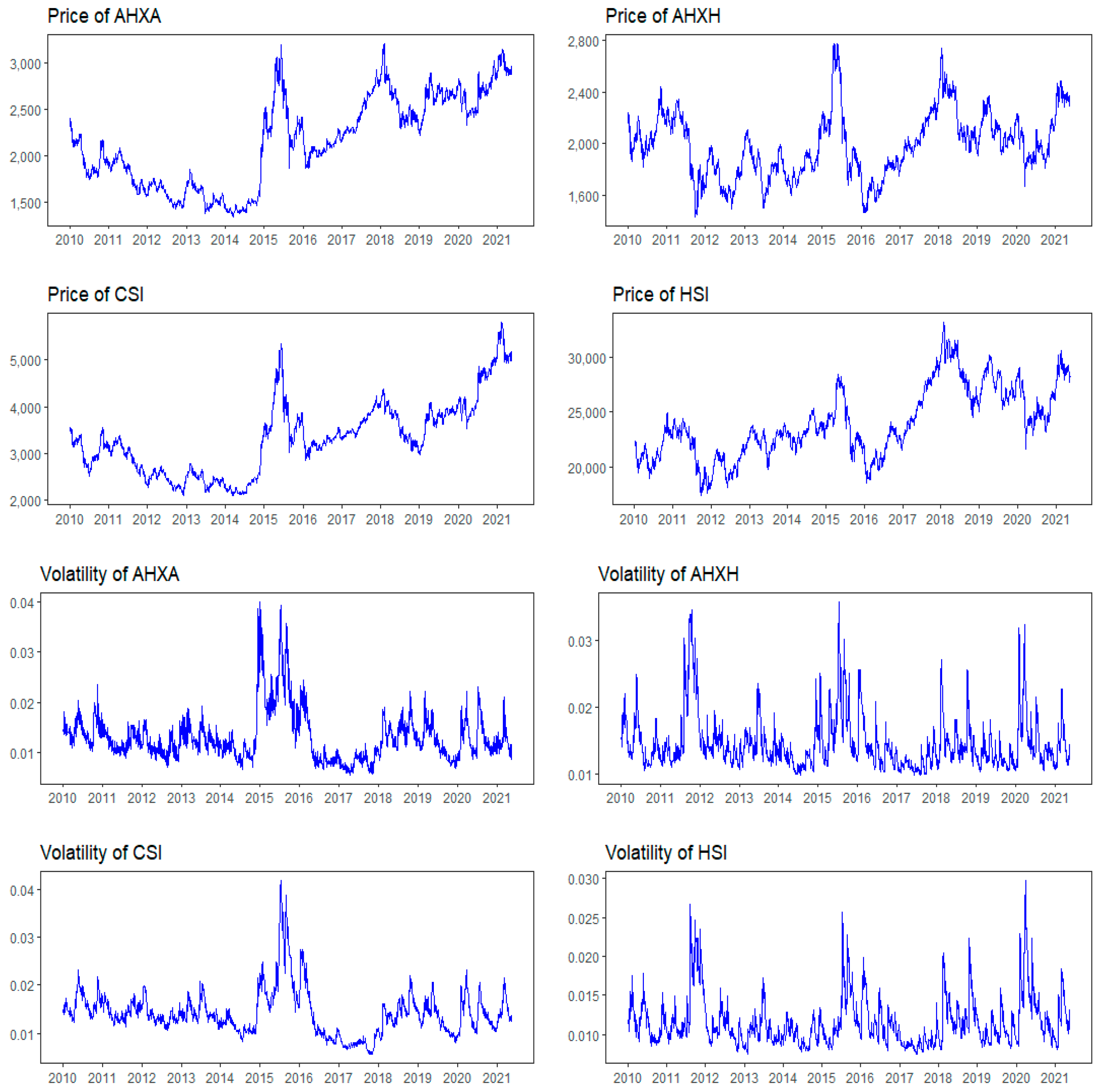
3.1. Data Description

This article examines the time-varying causalities for AHXA-AHXH pairing and CSI 300-HSI pairing at both price and volatility levels. At the price level, we use the daily log prices of the four indices from 4 January 2010 to 17 May 2021, covering 2680 observations. All these variables are obtained from Wind China. At the volatility level, the true volatility series cannot be obtained directly because of the invisible characteristics. This article follows the ARMA-GARCH procedure to get the daily fitted volatilities.

To obtain the fitted volatilities, we start by differencing the log price data into return series and checking the stationarity of the log-return series. To do this, two traditional unit root tests, namely the Augmented Dickey-Fuller (ADF) test and the Phillips–Perron (PP) test are implemented for all four return series. According to the results of the ADF tests and the PP tests, ARMA model is appropriate to capture the conditional mean of the log-return series. When fitting the four log-return series with sparse ARMA model, this article chooses the best AR order and MA order based on three criteria (the maximum AR order and MA order are both 10 in our experiment). First, all the estimated parameters should be statistically significant at 5% significance level. Second, the residuals should be white noise (we use the Box-Ljung test to assess whether the residual series is white noise or not). Third, the Bayesian Information Criterion (BIC) should be the minimum among all feasible models. Afterward, the residuals of the ARMA models are extracted to fit the GARCH model. This paper also uses two criteria to obtain the best GARCH model for these residual series (we employ GARCH, EGARCH, GJR-GARCH models for alternative models and normal distribution, Student-t distribution for alternative distributions). First, the standard residuals, which are calculated as the residuals divided by the fitted volatilities, should be homoscedasticity (we use the LM statistics to test the existence of heteroskedasticity in the standard residual series). Second, the BIC should be the minimum among all feasible models. The best ARMA and GARCH models for four log-return series are shown in

Table 1. Best ARMA-GARCH models for fitting log-return series.

Index	Mean Model	GARCH Model
AHXA	Sparse ARMA(5,3) (AR2 and AR4 fixed at 0)	EGARCH(2,2) (Normal distribution)
AHXH	ARMA(1,0)	GJR-GARCH(2,1) (t distribution)
CSI	Sparse ARMA(4,4) (AR1, MA1, and MA2 fixed at 0)	EGARCH(1,1) (t distribution)
HSI	ARMA(2,2)	EGARCH(2,1) (t distribution)

. Then, we can obtain the daily volatilities from the models for these four variables.

Figure 1 plots the price series and the volatility series of the four indices during the sample period. The first two rows of Figure 1 show that the prices of AHXA and AHXH indices have similar trends to those of CSI and HSI indices, respectively. It preliminarily indicates that the cross-listed stocks are likely to be affected by their market environments. On one hand, the Chinese mainland stock indices (CSI, AHXA) exhibit a fluctuated downward trend from the start point of our sample to mid-2014. Hereafter, two indices experience a dramatic surge followed by a crash in 2015 and 2016. After that, the Chinese mainland stock indices go through fluctuating rise until the end of the sample period. On the other hand, the Hong Kong stock indices (HSI, AHXH) fluctuate sharply throughout the sample. They experience a slump in early 2016 and then quickly climb and arrive at their peak in 2018. Notably, the Hong Kong stock indices dropped dramatically when the COVID-19 pandemic broke out in early 2020 but soon recovered rapidly, while the Chinese mainland stock indices seem to be immune to the pandemic and change at their own pace. The last two rows of Figure 1 describe the movements of volatility series for these four indices. As can be seen, when the price series experience large changes, the corresponding fitted volatilities are high. On the contrary, when the price series do not fluctuate much, the corresponding fitted volatilities are low. This shows the stylized volatility clustering, indicating that the ARMA-GARCH model is suitable to fit the volatilities of these four indices.

The descriptive analysis and some basic tests for all price, return, and volatility data are provided in

Table 2. Descriptive statistics.

	Mean	Std. Dev.	Skewness	Kurtosis	JB
Price
CSI	3320.952	787.512	0.567 *	2.935	144.137 *
AHXA	2158.179	486.335	0.046	1.795 *	162.776 *
AHXH	1971.335	250.006	0.410 *	2.997	79.291 *
HSI	24,064.616	3186.906	0.404 *	2.422 *	109.918 *
Return
CSI	0.000143	0.014934	−0.654 *	4.902 *	2880.361 *
AHXA	0.000083	0.014140	−0.321 *	6.215 *	4366.804 *
AHXH	0.000034	0.015164	−0.064	2.779 *	866.445 *
HSI	0.000096	0.011932	−0.318 *	2.735 *	882.803 *
Volatility
CSI	0.014	0.005	1.637 *	8.355 *	4406.751 *
AHXA	0.013	0.005	1.881 *	8.189 *	4594.585 *
AHXH	0.015	0.004	1.991 *	7.668 *	4210.519 *
HSI	0.012	0.003	1.758 *	6.779 *	2979.322 *

* indicates significance at 5% level.

. The mean of the AHXA (2158.18) is much higher than that of the AHXH (1971.34), which indicates that the AH premium puzzle may still exist throughout the sample interval. The means of the volatility series for all indices are ranged from 1.2 to 1.5%, which are roughly the same. That is to say, all indices have similar volatilities under the normal market environments. Meanwhile, all the price series (except for AHXA) and all the volatility series are positively skewed and all the return series (except for AHXH) are negatively skewed according to the skewnesses. All the series statistically reject the null hypothesis of normal distribution at 1% significance level as indicated by the Jarque–Bera (JB) test.

3.2. Methodology

In this part, we briefly introduce the time-varying causality test based on the REW algorithm and LA-VAR model developed by Shi et al. [18,19] (the test based on the VAR model is much similar so we do not repeat introduce it). Let ${\mathit{y}}_t$ be a k-dimension (k = 4 in this paper) column vector at time t. Then, $\mathit{Y}={({\mathit{y}}_1,\dots ,{\mathit{y}}_T{)}^{\prime }}_{T\times k}^{}$ is a k-vector time series, which have T observations. Thus, at a given time point t, the LA-VAR (q + d) model can be written as

$${\mathit{y}}_t={\mathit{\alpha }}_0+{\mathit{\alpha }}_{1}t+{\displaystyle \sum _{i=1}^q{\mathit{\beta }}_i}{\mathit{y}}_{t-i}+{\displaystyle \sum _{j=q+1}^{q+d}{\mathit{\delta }}_j}{\mathit{y}}_{t-j}+{\mathit{\epsilon }}_t,$$

(1)

where t represents the time trend, q is the lag order for the initial VAR model based on BIC, d is the maximum integration order for $\mathit{Y}$. ${\mathit{\epsilon }}_t$ is the error term, ${\mathit{\alpha }}_0$, ${\mathit{\alpha }}_1$, ${\mathit{\beta }}_i$, ${\mathit{\delta }}_j$ are all k-dimension column vectors. Equation (1) can be rewritten as

$$\mathit{Y}=\mathit{\tau }{\mathit{\Gamma }}^{\prime }+\mathit{X}{\mathit{\Phi }}^{\prime }+\mathit{Z}{\mathit{\Psi }}^{\prime }+\mathit{\epsilon },$$

(2)

where $\mathit{\tau }={({\mathit{\tau }}_1,\dots ,{\mathit{\tau }}_T)}_{T\times 2}^{\prime }$, ${\mathit{\tau }}_t={(1,t)}_{2\times 1}^{\prime }$; $\mathit{\Gamma }={({\mathit{\alpha }}_0,{\mathit{\alpha }}_1)}_{k\times 2}$; $\mathit{X}={({\mathit{x}}_1,\dots ,{\mathit{x}}_T)}_{T\times kq}^{\prime }$, ${\mathit{x}}_t={({\mathit{y}}_{t-1}^{\prime },\dots ,{\mathit{y}}_{t-q}^{\prime })}_{kq\times 1}^{\prime }$; $\mathit{Z}={({\mathit{z}}_1,\dots ,{\mathit{z}}_T)}_{T\times kd}^{\prime }$, ${\mathit{z}}_t={({\mathit{y}}_{t-q-1}^{\prime },\dots ,{\mathit{y}}_{t-q-d}^{\prime })}_{kd\times 1}^{\prime }$; $\mathit{\Phi }={({\mathit{\beta }}_1,\dots ,{\mathit{\beta }}_q)}_{k\times kq}$; $\mathit{\Psi }={({\mathit{\delta }}_{q+1},\dots ,{\mathit{\delta }}_{q+d})}_{k\times kd}$; $\mathit{\epsilon }={({\mathit{\epsilon }}_1,\dots ,{\mathit{\epsilon }}_T)}_{T\times k}^{\prime }$.

In this model, we take Ordinary Least Squares (OLS) estimators for parameters $\mathit{\Phi }$. The estimated results can be expressed as $\hat{\mathit{\Phi }}={\mathit{Y}}^{\prime }\mathit{Q}\mathit{X}{({\mathit{X}}^{\prime }\mathit{Q}\mathit{X})}^{-1}$, where $\mathit{Q}={\mathit{Q}}_{\mathit{\tau }}-{\mathit{Q}}_{\mathit{\tau }}\mathit{Z}{({\mathit{Z}}^{\prime }{\mathit{Q}}_{\mathit{\tau }}\mathit{Z})}^{-1}{\mathit{Z}}^{\prime }{\mathit{Q}}_{\mathit{\tau }}$, ${\mathit{Q}}_{\mathit{\tau }}={\mathit{I}}_T-\mathit{\tau }{({\mathit{\tau }}^{\prime }\mathit{\tau })}^{-1}{\mathit{\tau }}^{\prime }$. After getting the estimated results, a basic causality test can be further conducted. The null hypothesis of Granger non-causality can be expressed as

$$H_0:\mathit{R}\mathit{\phi }=0,$$

(3)

where $\mathit{\phi }=\mathrm{vec}(\mathit{\Phi })$ using row vectorization, so $\mathit{\phi }$ is a row vector with length $k^{2}q$. $\mathit{R}$ is a $m\times k^{2}q$ matrix where m represents the number of restrictions in the null hypothesis. All elements in $\mathit{R}$ are composed of 0 and 1, which are used to control the necessary parameters in the test. Based on the null hypothesis, the Wald statistic can be written as

$$\mathcal{W}=(\mathit{R}\hat{\mathit{\phi }}{)}^{\prime }{\{\mathit{R}[\hat{\mathit{\Omega }}\otimes {({\mathit{X}}^{\prime }\mathit{Q}\mathit{X})}^{-1}]{\mathit{R}}^{\prime }\}}^{-1}(\mathit{R}\hat{\mathit{\phi }}), \hat{\mathit{\phi }}=\mathrm{vec}(\hat{\mathit{\Phi }}),\hat{\mathit{\Omega }}=\frac{{\hat{\mathit{\epsilon }}}^{\prime }\hat{\mathit{\epsilon }}}{T},$$

(4)

where $\otimes$ is the Kronecker product. The Wald statistic is asymptotically ${\chi }_m^2$ distributed. If the Wald statistic is higher than the corresponding critical value, the causal relationship exists between the series being tested.

Based on the Wald statistic and the REW algorithm, Shi et al. [18,19] suggest a sup Wald test. Assume $f_1$ and $f_2$ represent the begin point and end point of the target window, respectively, and $0\le f_1\le f_2\le 1$. Let $f_{\mathit{w}}=f_2-f_1$, which represents the sample size fraction. Here, we set a minimum sample size $f_0$ for $f_{\mathit{w}}$ to ensure the LA-VAR system can be estimated (a suggested value for by Shi et al. (2020) is one-fifth of the sample size). Then the Wald test from $f_1$ to $f_2$ with a size fraction of $f_{\mathit{w}}$ is denoted by ${\mathcal{W}}_{f_1}^{f_2}$, and the sup Wald statistic at point $f_{}$ is given by

$$\mathcal{S}{\mathcal{W}}_f(f_0)=\underset{f_2=f,f_1\in [0,f_2-f_0]}{\sup }\left\{{\mathcal{W}}_{f_1}^{f_2}\right\}.$$

(5)

Then, $T-\lfloor T\times f_0\rfloor +1$ sup Wald statistics can be figured out where $f_{}$ evolves from $f_0$ to 1. These statistics are matched with time region $[\lfloor T\times f_0\rfloor ,T]$. For these sup Wald statistics, we set only one critical value (scv) using the bootstrap method. If the sup Wald statistic at time t is higher than scv, that is $\mathcal{S}{\mathcal{W}}_{f_t}(f_0)\ge scv$, $t=T\times f_t$, then the causality relationship holds at time t.

This test is useful to judge whether causalities exist between two variables over time. However, it is unable to assess whether the underlying causalities are positive or negative. As aforementioned, the sup Wald statistic is the maximum value of a sequence of Wald statistics, so there is a $f_{*}$ that satisfy the following equation.

$${\mathcal{W}}_{f_{*}}^{f_t}=\underset{f_2=f,f_1\in [0,f_2-f_0]}{\sup }\left\{{\mathcal{W}}_{f_1}^{f_2}\right\}=\mathcal{S}{\mathcal{W}}_{f_t}(f_0).$$

(6)

At time t, if there exists causality between two variables, that is $\mathcal{S}{\mathcal{W}}_{f_t}(f_0)\ge scv$, then we can further judge whether the underlying causality is positive or not by looking at the sign of the parameters being tested ($\mathit{R}\hat{\mathit{\phi }}$), where the $\hat{\mathit{\phi }}$ is the OLS estimators using observation intervals $[\lfloor T\times f_{*}\rfloor ,\lfloor T\times f_t\rfloor ]$.

4. Results and Discussions

4.1. Maximum Order of Integration

To implement the time-varying causality test, we check the maximum integration order for price series and volatility series first. Here, we employ ADF and PP tests for this aim. Both tests are performed for all series at the level and at the first difference. The results of these tests are reported in

Table 3. Results of unit root tests.

		$\mathbf{ln}{\mathit{P}}_{\mathit{C}\mathit{S}\mathit{I}}$	$\mathbf{ln}{\mathit{P}}_{\mathit{A}\mathit{H}\mathit{X}\mathit{A}}$	$\mathbf{ln}{\mathit{P}}_{\mathit{A}\mathit{H}\mathit{X}\mathit{H}}$	$\mathbf{ln}{\mathit{P}}_{\mathit{H}\mathit{S}\mathit{I}}$	${\mathit{V}\mathit{o}\mathit{l}}_{\mathit{C}\mathit{S}\mathit{I}}$	${\mathit{V}\mathit{o}\mathit{l}}_{\mathit{A}\mathit{H}\mathit{X}\mathit{A}}$	${\mathit{V}\mathit{o}\mathit{l}}_{\mathit{A}\mathit{H}\mathit{X}\mathit{H}}$	${\mathit{V}\mathit{o}\mathit{l}}_{\mathit{H}\mathit{S}\mathit{I}}$
Level
ADF	Intercept	0.6046	0.5956	0.0212 *	0.2116	<0.01 *	<0.01 *	<0.01 *	<0.01 *
	Intercept and Trend	0.2505	0.1942	0.0442 *	0.0596	<0.01 *	<0.01 *	<0.01 *	<0.01 *
PP	Intercept	0.8998	0.8834	0.0564	0.5175	<0.01 *	<0.01 *	<0.01 *	<0.01 *
	Intercept and Trend	0.3944	0.3247	0.0312 *	0.0368 *	<0.01 *	<0.01 *	<0.01 *	<0.01 *
First difference
ADF	Intercept	<0.01 *	<0.01 *	<0.01 *	<0.01 *	<0.01 *	<0.01 *	<0.01 *	<0.01 *
	Intercept and Trend	<0.01 *	<0.01 *	<0.01 *	<0.01 *	<0.01 *	<0.01 *	<0.01 *	<0.01 *
PP	Intercept	<0.01 *	<0.01 *	<0.01 *	<0.01 *	<0.01 *	<0.01 *	<0.01 *	<0.01 *
	Intercept and Trend	<0.01 *	<0.01 *	<0.01 *	<0.01 *	<0.01 *	<0.01 *	<0.01 *	<0.01 *
Conclusion		$I(1)$	$I(1)$	$I(0)$	$I(1)$	$I(0)$	$I(0)$	$I(0)$	$I(0)$

* indicates significance at 5% level.

. As indicated by the p values, all the tests for the first difference series significantly reject the null hypothesis. It shows that the integration order for all series would be either 0 or 1. Furthermore, none of the unit root tests reject the null hypothesis for two price series (CSI and AHXA), which means the two price series are not stationary. In addition, all the volatility series are stationary because all the unit root tests statistically reject the null hypothesis. Consequently, the maximum integration order d for the four-variable system at the price level is 1, while that at the volatility level is 0. Therefore, we conduct an LA-VAR model to test the time-varying causality at the price level and implement a stationary VAR model to detect the dynamic causal relationship at the volatility level.

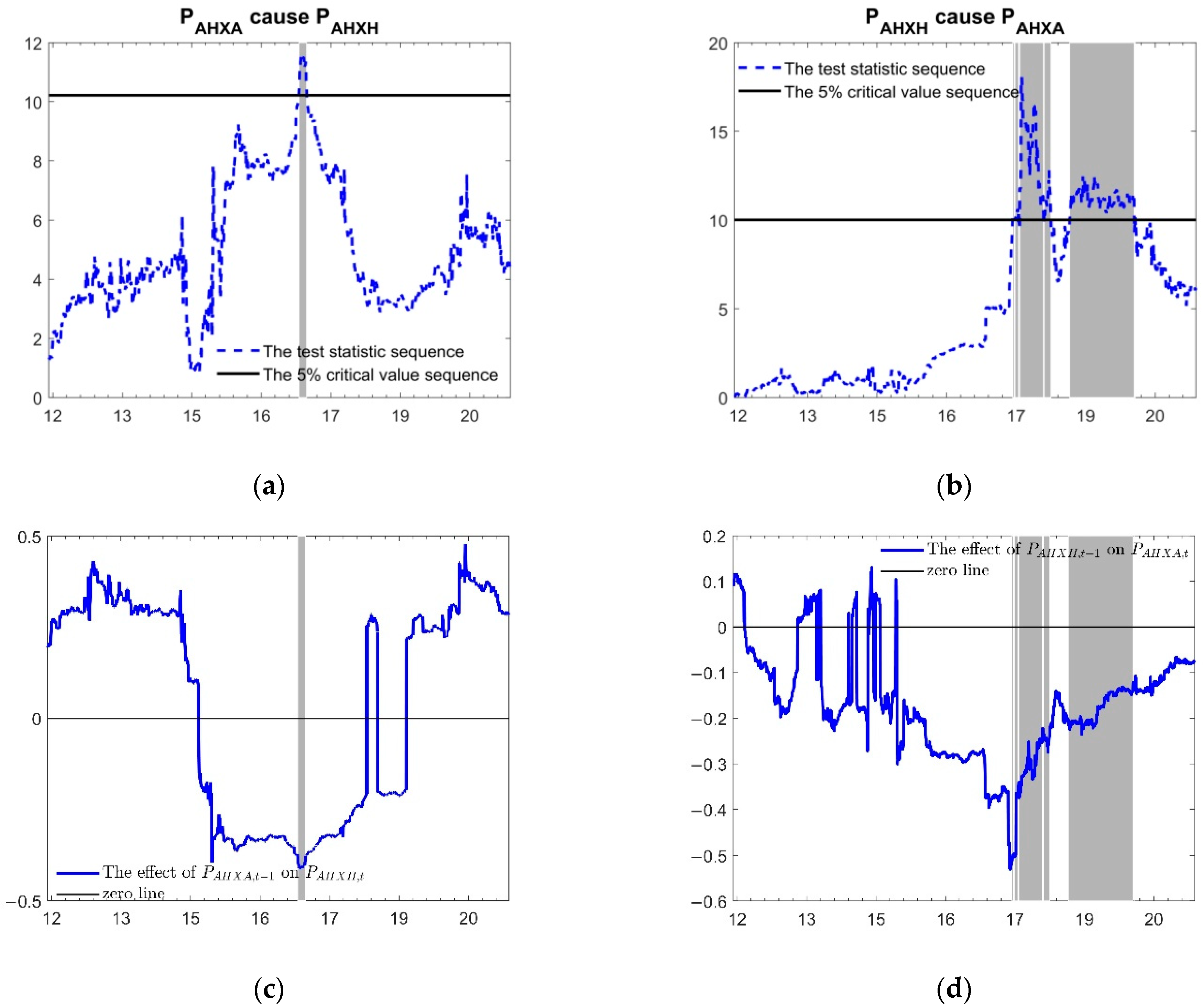
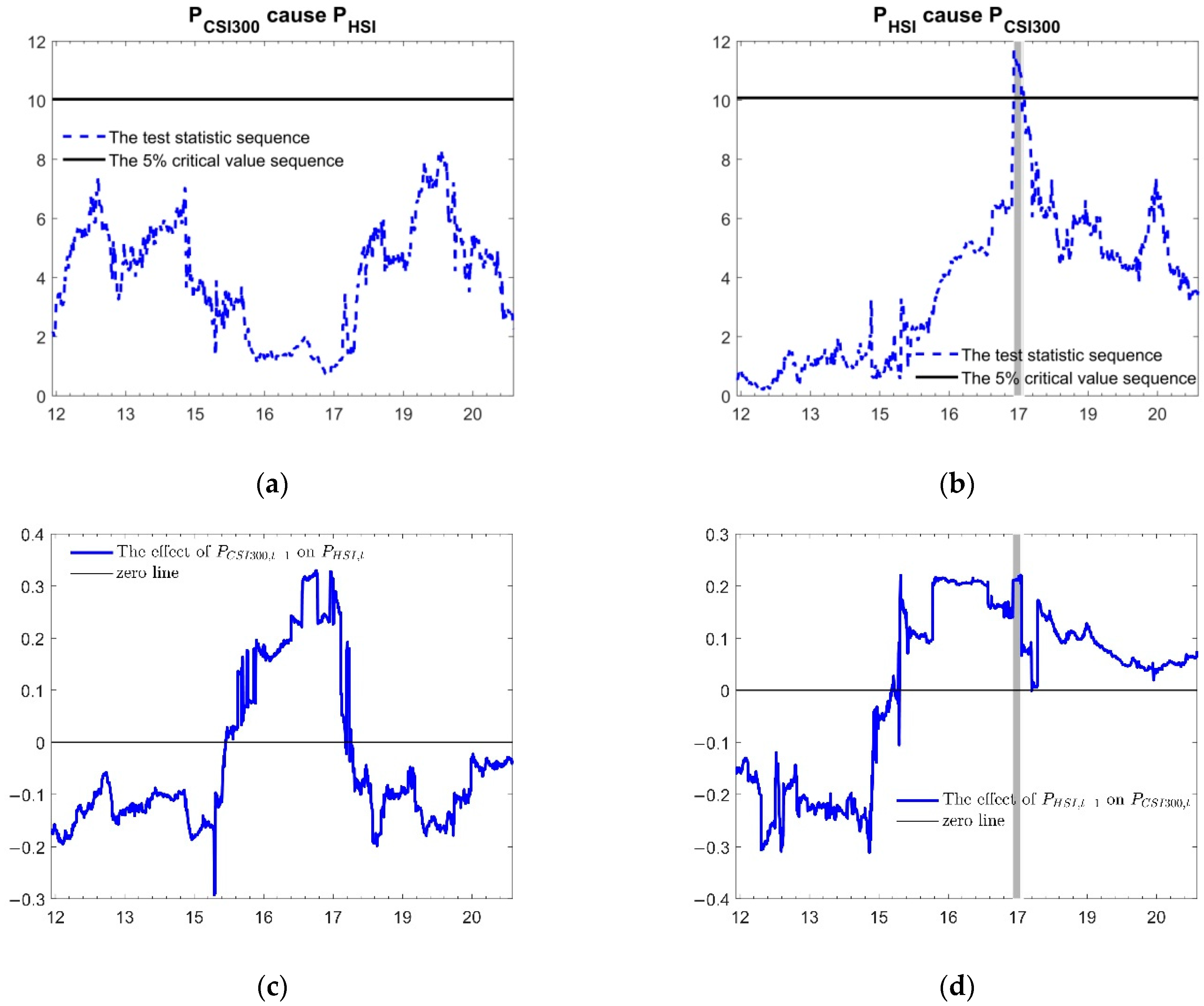
4.2. Time Varying Granger Test between Price Series

In this part, we construct a four-variable system using the log prices of the above indices and transport this system to the time-varying causality test based on the REW algorithm and LA-VAR model. The optimal lag order q of the initial VAR model equals 1 (BIC = −1.0299), and the maximum integration order d equals 1. Therefore, based on the LA-VAR (2) model, we apply the test for AHXA-AHXH pairing and for CSI 300-HSI pairing to assess how the one-period (q without d) lagged explanatory variable causes the explained variable over time. In addition, the heteroscedasticity is significant for both price and volatility series, as suggested by Figure 1. This article applies the time-varying causality test under the assumption of heteroscedasticity.

Figure 2 and Figure 3 display the results of the dynamic causalities for two price pairings (AHXA-AHXH, CSI 300-HSI). All the significant causality regions are marked in grey. As for the AHXA-AHXH pairing, panels (a) and (b) of Figure 2 exhibit the causality periods and the corresponding causality directions. In general, the causal relationships between $P_{AHXA}$ and $P_{AHXH}$ are concentrated in March 2017–February 2020, and the causalities are mainly transmitted from $P_{AHXA}$ to $P_{AHXH}$. Specifically, $P_{AHXA}$ unidirectionally causes $P_{AHXH}$ from 17 March to 12 May 2017. Afterward, this causal direction reverses soon. Significant causal relations run from $P_{AHXH}$ to $P_{AHXA}$ covering many periods, including 9 October 2017–20 October 2017, 26 October 2017–20 November 2017, 22 November 2017–23 November 2017, 28 November 2017–17 May 2018, 23 May 2018–10 June 2018, and 20 November 2018–27 February 2020.

From the intricate causalities, this paper refines three interesting conclusions. First, there is no causal relationship between two AH prices from the beginning of the sample to March 2017. It shows that there is no predictive power between the two prices during this period, and the A-share market and the H-share market do not affect each other when participating in the same asset pricing process. One possible reason is that during this period, the segmentation between the two stock markets still exists. Although the SHSC program launched on 17 November 2014 allows AH stocks to be traded by mainland and Hong Kong investors in both markets, due to the daily quota limitation of this program and the different transaction regulations between two markets (for example, T + 1 rule in mainland and T + 0 rule in Hong Kong; 10% daily price fluctuation limit in mainland and no limitation in Hong Kong), capital flows between two markets are subject to great restrictions. According to Zhang et al. [64], the daily transaction volume of the SHSC program is lower than 10% of the daily quota on most trading days. It is reasonable that two prices of AH stocks exhibit no causalities during this period. However, the causal relationship has occurred since March 2017, a few months after the launch of the SZSC program (The SZSC program was launched on 5 December 2016). This may result from the cumulative effect of both SHSC and SZSC programs. Rather than a single program, two programs work together to strengthen the linkages between two markets and thus affect each other when the AH stocks are priced. These results are in line with Wang [65] and Li and Chen [66]. Second, significant causalities between two AH prices appear from March 2017 to February 2020 except for several months and the direction of causalities is mainly from $P_{AHXH}$ to $P_{AHXA}$. It provides evidence that the prices of AH stocks in the H-share market may help to predict those in the A-share market. Moreover, it also implies that the H-share market has a price guidance effect on the A-share market when pricing for the same asset. In detail, $P_{AHXA}$ preliminary unidirectional causes $P_{AHXH}$ for two months, which may be attributed to the home market advantage (Almost all companies listed on the A-share market and the H-share market are registered in Chinese mainland. Thus, the A-share market is generally the home market and the H-share market is the host market). More precisely, home market investors get more information about cross-listed companies and react much faster than host market investors [34,67]. However, the causality direction later reverses quickly. $P_{AHXH}$ is a cause of $P_{AHXA}$ over the next three years. This might be due to the immaturity of the A-share market relative to the H-share market [2] and the irrational Chinese mainland investors compared to Hong Kong investors [64]. Although Hong Kong investors get the news later than Chinese mainland investors, they are good at incorporating the information into prices. Thus, $P_{AHXH}$ leads $P_{AHXA}$. Cai et al. [16] and Dzhambova et al. [17] give similar results. It is worth noting that the causal relationship has been temporarily interrupted from 11 July 2018 to 19 November 2018. One possible reason is that on 11 July 2018, the United States Trade Representative imposed an additional 10% tariff for 200 billion dollars Chinese products, which may severely hit the confidence of international investors in Chinese companies and thus pay less attention to Chinese stocks. Afterward on 1 December 2018, China and the United States reached a consensus to suspend the new tariffs at the G20 summit in Argentina. This might be a signal that international investors restart to focus on Chinese stocks. Third, the causal relationship between $P_{AHXA}$ and $P_{AHXH}$ disappears after February 2020. This is exactly the time when the COVID-19 pandemic broke out. It implies that the epidemic may sever the causal relationship between different AH stock prices of the two markets. One possible explanation is the investor panic resulting from the market crashes. According to Ding et al. [68], in the first quarter in 2020, many main stock indices fell more than 30%. The market crashes lead to panic sentiment across investors all over the world [69]. On one hand, the relatively immature mainland investors, which are mainly constituted by retail investors, tend to overreact to market crashes [70]. The irrational behavior of Chinese mainland investors may eliminate the price guidance effect from the H-share market and hence destroy the price causal relationship. On the other hand, as market crashes occur all over the world, both domestic and international investors have to transfer their funds to some safe markets, such as traditional precious metal markets and the cryptocurrency markets [71]. The capital withdrawn from stock markets leads to fewer interactions between A-share and H-share investors, indicating a cease of the causal relationship. This result is in line with Xue and Zhou [72] and Gluzman [73], who argue that causal linkage can be cleanly disentangled by exogenous shocks.

Panels (c) and (d) of Figure 2 further explain whether the effects of the causalities are positive or negative. As introduced above, we assess how the one-period (q without d) lagged explanatory variable causes the explained variable over time. In the grey zone, the causalities between $P_{AHXA}$ and $P_{AHXH}$ are negative. Given the causality direction from $P_{AHXH}$ to $P_{AHXA}$ and the AH premium situation, we summarize that the rise (decrease) of $P_{AHXH}$ leads to a fall of $P_{AHXA}$, which further narrows (widens) the AH premium.

As a comparison, this article also analyzes the causal relationship between the prices of major stock indices (CSI 300, HSI) in the two stock markets. Panels (a) and (b) of Figure 3 show that there is no significant causal relationship from $P_{CSI300}$ to $P_{HSI}$ in the whole sample, while $P_{HSI}$ only significantly causes $P_{CSI300}$ in small time intervals, including 27 September 2017–22 November 2017 and 28 November 2017–7 December 2017. From panels (c) and (d) of Figure 3, we know that $P_{HSI}$ has a slight positive effect on $P_{CSI300}$ in the grey zone. This shows that the Hong Kong stock market has a positive predictive ability for the mainland stock market in very short periods. As a whole, the causal relationships between the prices of CSI 300 and HSI do not hold for most sample periods. These findings differ from the results of Ge and Lin [74], which apply convergent cross-mapping method finding a gradually increasing bidirectional causal relationship between HSI and Chinese mainland stock indices after the Global financial crisis. This might be due to two reasons. First, the way we quantify the causal relationship is the time-varying causality test of Shi et al. [18,19] rather than the convergent cross-mapping method. Second, we take AHXA and AHXH into consideration when capturing the causality between CSI 300 and HSI. It is worth mentioning that there is a huge difference between the causal relationship of AHXA-AHXH pairing and that of CSI 300-HSI pairing at the price level. This is strong evidence indicating that the time-varying causal relationship between cross-listed submarkets is independent of that between two major markets at the price level.

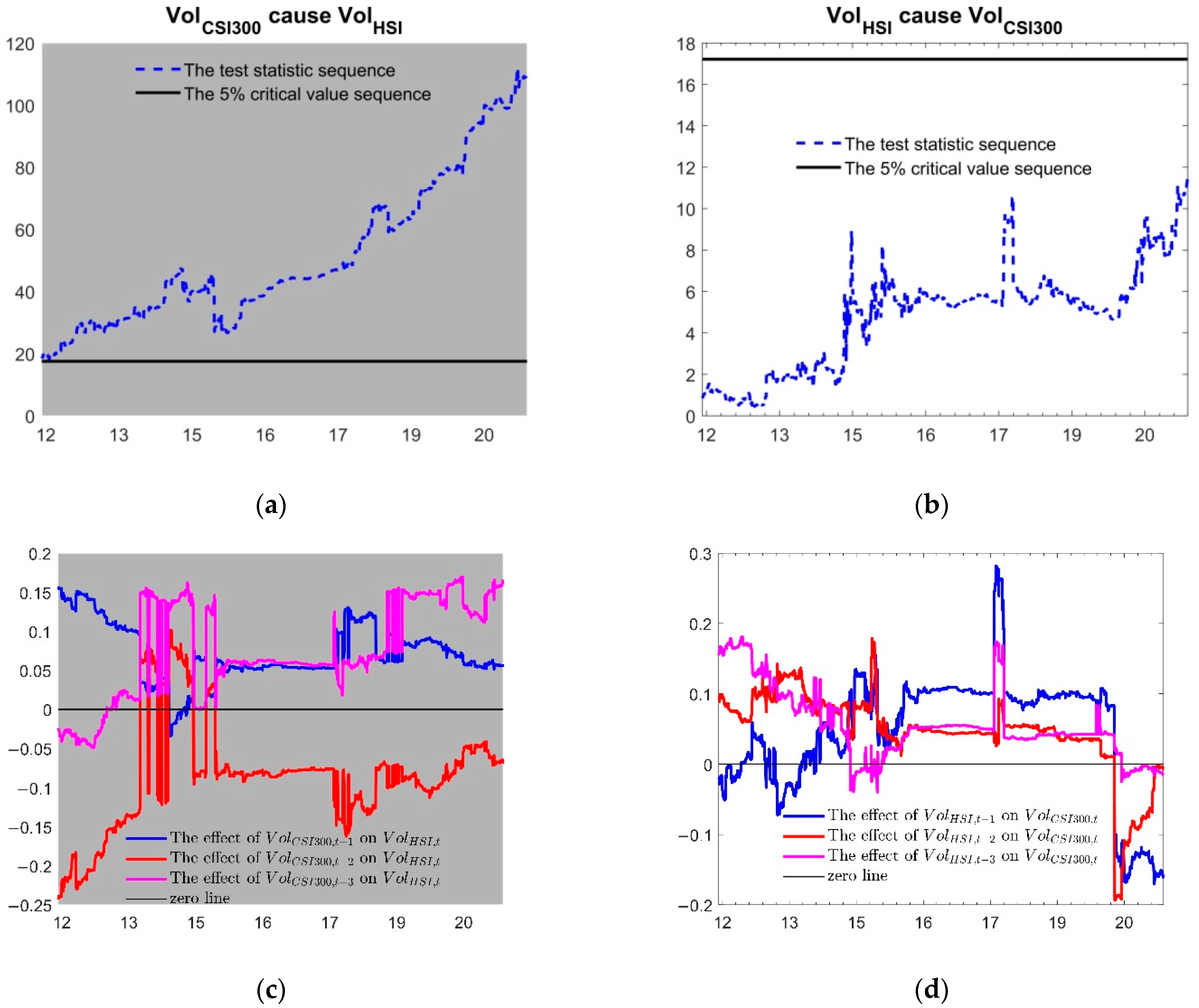
4.3. Time Varying Granger Test between Volatility Series

In this part, we detect the causal relationship for AHXA-AHXH pairing and CSI 300-HSI pairing at the volatility level. The procedure is similar to the test at the price level. The optimal lag order q of the initial VAR model equals 3 (BIC = −1.5463), and the maximum integration order d equals 0. So, a stationary VAR (3) model is used. In other words, we assess how the three-period lagged explanatory variables cause the explained variable over time for these two pairings at the volatility level.

The causalities of the two pairings at the volatility level shown in Figure 4 and Figure 5 are much different from those at the price level. As displayed in panels (a) and (b) of Figure 4, the volatilities of AHXH exert no causal effects on the volatilities of AHXA over the whole sample period. On the contrary, significant causalities run from the volatilities of AHXA to the volatilities of AHXH covering many intervals, including 15 April 2014–24 April 2014, 5 May 2014–8 May 2014, 13 May 2014–21 January 2015, 3 February 2015, and 5 February 2015–17 May 2021. In general, significant volatility spillovers from the A-share market to the H-share market for AH stocks exist since April 2014. Furthermore, according to the causality effects displayed in panels (c) and (d) of Figure 4, all three lagged terms of $Vo{l}_{AHXA}$ draw significantly positive effects on $Vo{l}_{AHXH}$. That is to say, as the volatility of AHXA increases (decreases), the volatility of AHXH will soon increase (decrease) asynchronously. Finally, a fascinating result is that the causality direction at the volatility level is opposite to that at the price level. Although the H-share market provides price guidance for the A-share market when they participate in the price discovery process of the same assets, the volatility spillovers are transmitted from the A-share market to the H-share market. The home market advantage may also account for this. It is convenient for Chinese mainland investors to obtain extreme news about AH stocks. In a short time, they would transmit the information into prices and exert huge volatilities. This process would be so quick that international investors react relatively slow.

Moreover, this paper investigates the time-varying causalities between CSI 300 and HSI at the volatility level, aiming to make a comparison with those of AHXA-AHXH pairing. The graphical results are pictured in Figure 5. During the entire sample period, $Vo{l}_{CSI300}$ is a significant cause of $Vo{l}_{HSI}$, but not vice versa. It demonstrates that there are volatility spillovers from the A-share market to the H-share market. This is in line with Huo and Ahmed [75]. In addition, the impacts of $Vo{l}_{CSI300,t-2}$ on $Vo{l}_{HSI,t}$ are negative in most periods, while the impacts of $Vo{l}_{CSI300,t-1}$ and $Vo{l}_{CSI300,t-3}$ on $Vo{l}_{HSI,t}$ are mainly positive during the sample periods. At the volatility level, the causality directions are from the A-share market to the H-share market for both AHXA-AHXH pairing and CSI 300-HSI pairing. The high degree of consistency between them convinces us that the spillovers of cross-listed stocks probably result from the spillovers of the major stock markets. Overall, volatility spillovers are mainly transmitted from the Chinese mainland stock markets (CSI, AHXA) to the Hong Kong stock markets (HSI, AHXH). This means that when the Hong Kong stock markets are faced with a financial crisis, the Chinese mainland stock markets would be immune to the contagion effect. Unlike the causalities at the price level, the extreme events (the Chinese stock crash in 2015 and the COVID-19 pandemic in 2020) do not destroy the existing causal relationship at the volatility level. This is reasonable. When the extreme events followed by the market crashes occur, the correlations among stock markets increase significantly [31,76,77] and the market connectedness is much higher compared to that in normal market situations [78]. All these crisis features strengthen the financial contagion effects and volatility spillover effects [79], hence the causal relationships between A-share and H-share markets at the volatility level are still significant.

5. Conclusions

The launch of the SHSC program and the SZSC program in recent years has broadened the channels for the Chinese mainland and international investors to directly invest in AH stocks, which gradually eliminates the market segmentation between the Chinese mainland stock market and the Hong Kong stock market. However, the AH stocks still have different exchange-adjusted prices in different markets, that is, the AH premium puzzle. Given the AH premium puzzle, the investigation of the causal relationships between two prices in two markets enables one to understand the inner nexus about two stock markets and helps investors seek some arbitrage opportunities. In order to comprehensively examine the causal nexus between AH stocks in different markets, this article investigates the time-varying causal relationship between AH stocks at both price and volatility levels and further examines the dynamic causalities between major stock indices as a comparison. We apply a new time-vary causality technology proposed by Shi et al. [18,19] for our analysis.

The empirical results at the price level show that the causalities between two prices of AH stock indices do not exist all the time. The causality occurs from March 2017 to February 2020. During this period, negative causalities from the H-share markets to the A-share stock markets are the main feature. It implies that the H-share market has a price guidance effect on the A-share market when the same stocks are priced. Given the AH premium, an increase (decrease) in the price of H shares will guide the price of A shares to decrease (increase) significantly, thereby narrowing (widening) the AH premium. As a comparison, almost no causality exists between CSI 300 and HSI index at the price level over the whole period. The results at the volatility level are much different from those at the price level. In brief, volatility spillovers are transmitted from the Chinese mainland stock markets (CSI, AHXA) to the Hong Kong stock markets (HSI, AHXH). This means that when the Hong Kong stock markets are faced with a financial crisis, the Chinese mainland stock markets would be immune to the contagion effect. At last, this paper finds that the COVID-19 pandemic can destroy the causalities of AH stocks at price level while the causalities at the volatility level do not eliminate during the crises.

Our results have important implications for policymakers and investors. In recent years, the prices of AH stocks in the H-share market had a negative price prediction power for their prices in the A-share market. However, the prediction rules disappeared during the COVID-19 pandemic periods. If policymakers want to strengthen the linkage between the A-share market and the H-share market, they need to pay more attention to the AH cross-listed stocks. When policymakers make liberation policies that may reinforce the causal relationship between prices of AH stocks, investors in two markets will find more arbitrage opportunities and thus strengthen the relationship between two markets as well as leading to more efficient markets. Further research can focus on the reason why the causalities of AH stocks at the price level disappeared during the COVID-19 pandemic period.

References

1. Ding, Y.-J.; Feng, Y. The impact of market trading mechanism on A-H share price premium. Appl. Econ. Lett. 2018, 26, 594–600. [Google Scholar] [CrossRef]
2. Hui, E.C.M.; Chan, K.K.K. Does the Shanghai-Hong Kong stock connect significantly affect the A-H premium of the stocks? Physica A 2018, 492, 207–214. [Google Scholar] [CrossRef]
3. Pan, J.; Chi, J. How does the Shanghai-Hong Kong stock connect policy impact the A-H share premium? Emerg. Mark. Financ. Trade 2019, 57, 1912–1928. [Google Scholar] [CrossRef]
4. Pavlidis, E.G.; Vasilopoulos, K. Speculative bubbles in segmented markets: Evidence from Chinese cross-listed stocks. J. Int. Money Financ. 2020, 109, 102222. [Google Scholar] [CrossRef]
5. Luo, X.; Yu, X.; Qin, S.; Xu, Q. Option trading and the cross-listed stock returns: Evidence from Chinese A–H shares. J. Futures Mark. 2020, 40, 1665–1690. [Google Scholar] [CrossRef]
6. Huang, Z.; Gao, W. Stock market liberalization and firm litigation risk—A quasi-natural experiment based on the Shanghai-Hong Kong stock connect policy. Appl. Econ. 2021, 53, 5619–5642. [Google Scholar] [CrossRef]
7. Fan, Q.; Wang, T. The impact of Shanghai-Hong Kong stock connect policy on A-H share price premium. Financ. Res. Lett. 2017, 21, 222–227. [Google Scholar] [CrossRef]
8. Deng, L.; Liao, M.; Luo, R.; Sun, J.; Xu, C. Does corporate social responsibility reduce share price premium? Evidence from China’s A- and H-shares. Pac.-Basin Financ. J. 2021, 67, 101569. [Google Scholar] [CrossRef]
9. Cai, C.X.; McGuinness, P.B.; Zhang, Q. The pricing dynamics of cross-listed securities: The case of Chinese A- and H-shares. J. Bank. Financ. 2011, 35, 2123–2136. [Google Scholar] [CrossRef]
10. Eun, C.S.; Sabherwal, S. Cross-border listings and price discovery: Evidence from US-listed Canadian stocks. J. Financ. 2003, 58, 549–575. [Google Scholar] [CrossRef] [Green Version]
11. Frijns, B.; Indriawan, I.; Tourani-Rad, A. The interactions between price discovery, liquidity and algorithmic trading for U.S.-Canadian cross-listed shares. Int. Rev. Finan. Anal. 2018, 56, 136–152. [Google Scholar] [CrossRef]
12. Wu, L.; Xu, K.; Meng, Q. Information flow and price discovery dynamics. Rev. Quant. Financ. Acc. 2020, 56, 329–367. [Google Scholar] [CrossRef]
13. Bekhet, H.A.; Matar, A. Co-integration and causality analysis between stock market prices and their determinates in Jordan. Econ. Model. 2013, 35, 508–514. [Google Scholar] [CrossRef]
14. Bahmani-Oskooee, M.; Ghodsi, S.H. Asymmetric causality between the U.S. housing market and its stock market: Evidence from state level data. J. Econ. Asymmetries 2018, 18, e00095. [Google Scholar] [CrossRef]
15. Sun, X.; Fang, W.; Gao, X.; An, S.; Liu, S.; Wu, T. Time-varying causality inference of different nickel markets based on the convergent cross mapping method. Resour. Pol. 2021, 74, 102385. [Google Scholar] [CrossRef]
16. Cai, C.X.; McGuinness, P.B.; Zhang, Q. Capital account reform and short- and long-run stock price leadership. Europ. J. Financ. 2015, 23, 916–945. [Google Scholar] [CrossRef] [Green Version]
17. Dzhambova, K.; Tao, R.; Yuan, Y. Price leadership and asynchronous movements of multi-market listed stocks. Int. Rev. Finan. Anal. 2022, 79, 101970. [Google Scholar] [CrossRef]
18. Shi, S.; Hurn, S.; Phillips, P.C.B. Causal change detection in possibly integrated systems: Revisiting the money-income relationship. J. Financ. Econ. 2020, 18, 158–180. [Google Scholar] [CrossRef] [Green Version]
19. Shi, S.; Phillips, P.C.B.; Hurn, S. Change detection and the causal impact of the yield curve. J. Time Ser. Anal. 2018, 39, 966–987. [Google Scholar] [CrossRef] [Green Version]
20. Shahzad, F.; Bouri, E.; Mokni, K.; Ajmi, A.N. Energy, agriculture, and precious metals: Evidence from time-varying Granger causal relationships for both return and volatility. Resour. Pol. 2021, 74, 102298. [Google Scholar] [CrossRef]
21. Fang, L.; Chen, B.; Yu, H.; Qian, Y. The importance of global economic policy uncertainty in predicting gold futures market volatility: A GARCH-MIDAS approach. J. Futures Mark. 2018, 38, 413–422. [Google Scholar] [CrossRef]
22. Kambouroudis, D.S.; McMillan, D.G.; Tsakou, K. Forecasting stock return volatility: A comparison of GARCH, implied volatility, and realized volatility models. J. Futures Mark. 2016, 36, 1127–1163. [Google Scholar] [CrossRef]
23. Barucci, E.; Renò, R. On measuring volatility and the GARCH forecasting performance. J. Int. Finan. Mark. Inst. Money 2002, 12, 183–200. [Google Scholar] [CrossRef]
24. Satchell, S.; Knight, J. Forecasting Volatility in the Financial Markets, 3rd ed.; Elsevier: Oxford, UK, 2007; pp. 101–119. [Google Scholar]
25. Christopoulos, D.K.; Tsionas, E.G. Financial development and economic growth: Evidence from panel unit root and cointegration tests. J. Devel. Econ. 2004, 73, 55–74. [Google Scholar] [CrossRef]
26. Calderón, C.; Liu, L. The direction of causality between financial development and economic growth. J. Devel. Econ. 2003, 72, 321–334. [Google Scholar] [CrossRef] [Green Version]
27. Jalil, A.; Feridun, M. The impact of growth, energy and financial development on the environment in China: A cointegration analysis. Energy Econ. 2011, 33, 284–291. [Google Scholar] [CrossRef]
28. Hsueh, S.; Hu, Y.; Tu, C. Economic growth and financial development in Asian countries: A bootstrap panel Granger causality analysis. Econ. Model. 2013, 32, 294–301. [Google Scholar] [CrossRef]
29. Adekoya, O.B.; Oliyide, J.A. How COVID-19 drives connectedness among commodity and financial markets: Evidence from TVP-VAR and causality-in-quantiles techniques. Resour. Pol. 2021, 70, 101898. [Google Scholar] [CrossRef]
30. Afshan, S.; Sharif, A.; Nassani, A.A.; Abro, M.M.Q.; Batool, R.; Zaman, K. The role of information and communication technology (internet penetration) on Asian stock market efficiency: Evidence from quantile-on-quantile cointegration and causality approach. Int. J. Financ. Econ. 2020, 26, 2307–2324. [Google Scholar] [CrossRef]
31. Lin, A.; Shang, P.; Zhou, H. Cross-correlations and structures of stock markets based on multiscale MF-DXA and PCA. Nonlinear Dyn. 2014, 78, 485–494. [Google Scholar] [CrossRef]
32. Ruan, Q.; Zhang, S.; Lv, D.; Lu, X. Financial liberalization and stock market cross-correlation: MF-DCCA analysis based on Shanghai-Hong Kong stock connect. Physica A 2018, 491, 779–791. [Google Scholar] [CrossRef]
33. Harris, F.H.D.; McInish, T.H.; Shoesmith, G.L.; Wood, R.A. Cointegration, error correction, and price discovery on informationally linked security markets. J. Financ. Quant. Anal. 1995, 30, 563–579. [Google Scholar] [CrossRef]
34. Kehrle, K.; Peter, F.J. Who moves first? An intensity-based measure for information flows across stock exchanges. J. Bank. Financ. 2013, 37, 1629–1642. [Google Scholar] [CrossRef]
35. Su, Q.; Chong, T.T. Determining the contributions to price discovery for Chinese cross-listed stocks. Pac.-Basin Financ. J. 2007, 15, 140–153. [Google Scholar] [CrossRef]
36. Ma, J.; Swan, P.L.; Song, F. Price discovery and information in an emerging market: Evidence from China. In Proceedings of the 2009 China International Conference in Finance, Guangzhou, China, 7 July 2009. [Google Scholar]
37. Chan, M.K.; Kwok, S.S. Capital account liberalization and dynamic price discovery: Evidence from Chinese cross-listed stocks. Appl. Econ. 2015, 48, 517–535. [Google Scholar] [CrossRef]
38. Li, M.L.; Chui, C.M.; Li, C.Q. Is pairs trading profitable on China AH-share markets? Appl. Econ. Lett. 2014, 21, 1116–1121. [Google Scholar] [CrossRef]
39. Yuan, D.; Zhou, X.; Li, S. The dynamics of financial market integration between chinese A- and H-shares. Emerg. Mark. Financ. Trade 2018, 54, 2909–2924. [Google Scholar] [CrossRef]
40. Chen, H.; Zhu, Y. An empirical study on the threshold cointegration of Chinese A and H cross-listed shares. J. Appl. Statist. 2015, 42, 2406–2419. [Google Scholar] [CrossRef]
41. Tilfani, O.; Ferreira, P.; El Boukfaoui, M.Y. Dynamic cross-correlation and dynamic contagion of stock markets: A sliding windows approach with the DCCA correlation coefficient. Empir. Econ. 2019, 60, 1127–1156. [Google Scholar] [CrossRef]
42. Eryiğit, M.; Eryiğit, R. Network structure of cross-correlations among the world market indices. Physica A 2009, 388, 3551–3562. [Google Scholar] [CrossRef]
43. Ma, F.; Wei, Y.; Huang, D. Multifractal detrended cross-correlation analysis between the Chinese stock market and surrounding stock markets. Physica A 2013, 392, 1659–1670. [Google Scholar] [CrossRef]
44. Cao, G.; Zhou, L. Asymmetric risk transmission effect of cross-listing stocks between mainland and Hong Kong stock markets based on MF-DCCA method. Physica A 2019, 526, 120741. [Google Scholar] [CrossRef]
45. Xu, N.; Li, S. Segment stock market, foreign investors, and cross-correlation: Evidence from MF-DCCA and spillover index. Complexity 2020, 2020, 5836142. [Google Scholar] [CrossRef]
46. Kaufmann, R.K.; Ullman, B. Oil prices, speculation, and fundamentals: Interpreting causal relations among spot and futures prices. Energy Econ. 2009, 31, 550–558. [Google Scholar] [CrossRef]
47. Shrestha, K. Price discovery in energy markets. Energy Econ. 2014, 45, 229–233. [Google Scholar] [CrossRef]
48. Hallack, L.N.; Kaufmann, R.; Szklo, A.S. Price discovery in Brazil: Causal relations among prices for crude oil, ethanol, and gasoline. Energ. Source Part B 2020, 15, 230–251. [Google Scholar] [CrossRef]
49. Granger, C.W. Investigating causal relations by econometric models and cross-spectral methods. Econometrica 1969, 37, 424–438. [Google Scholar] [CrossRef]
50. Thoma, M.A. Subsample instability and asymmetries in money-income causality. J. Econom. 1994, 64, 279–306. [Google Scholar] [CrossRef]
51. Swanson, N.R. Money and output viewed through a rolling window. J. Monet. Econ. 1998, 41, 455–474. [Google Scholar] [CrossRef]
52. Arora, V.; Shi, S. Energy consumption and economic growth in the United States. Appl. Econ. 2016, 48, 3763–3773. [Google Scholar] [CrossRef]
53. Shi, G.; Liu, X.; Zhang, X. Time-varying causality between stock and housing markets in China. Financ. Res. Lett. 2017, 22, 227–232. [Google Scholar] [CrossRef]
54. Si, D.; Li, X.; Jiang, S. Can insurance activity act as a stimulus of economic growth? Evidence from time-varying causality in China. Emerg. Mark. Financ. Trade 2018, 54, 3030–3050. [Google Scholar] [CrossRef]
55. Phillips, P.C.; Shi, S.; Yu, J. Testing for multiple bubbles: Historical episodes of exuberance and collapse in the S&P 500. Int. Econ. Rev. 2015, 56, 1043–1078. [Google Scholar]
56. Phillips, P.C.; Shi, S.; Yu, J. Testing for multiple bubbles: Limit theory of real-time detectors. Int. Econ. Rev. 2015, 56, 1079–1134. [Google Scholar] [CrossRef] [Green Version]
57. Toda, H.Y.; Yamamoto, T. Statistical inference in vector autoregressions with possibly integrated processes. J. Econom. 1995, 66, 225–250. [Google Scholar] [CrossRef]
58. Hammoudeh, S.; Ajmi, A.N.; Mokni, K. Relationship between green bonds and financial and environmental variables: A novel time-varying causality. Energy Econ. 2020, 92, 104941. [Google Scholar] [CrossRef]
59. Emirmahmutoglu, F.; Denaux, Z.; Topcu, M. Time-varying causality between renewable and non-renewable energy consumption and real output: Sectoral evidence from the United States. Renew. Sust. Energ. Rev. 2021, 149, 111326. [Google Scholar] [CrossRef]
60. Chen, C.; Chiang, S. Time-varying causality in the price-rent relationship: Revisiting housing bubble symptoms. J. Hous. Built Environ. 2020, 36, 539–558. [Google Scholar] [CrossRef]
61. Hu, Y.; Hou, Y.G.; Oxley, L. What role do futures markets play in Bitcoin pricing? Causality, cointegration and price discovery from a time-varying perspective? Int. Rev. Finan. Anal. 2020, 72, 101569. [Google Scholar] [CrossRef]
62. Raggad, B. Time varying causal relationship between renewable energy consumption, oil prices and economic activity: New evidence from the United States. Resour. Pol. 2021, 74, 102422. [Google Scholar] [CrossRef]
63. Balcilar, M.; Ozdemir, Z.A.; Shahbaz, M. On the time-varying links between oil and gold: New insights from the rolling and recursive rolling approaches. Int. J. Finance Econ. 2019, 24, 1047–1065. [Google Scholar] [CrossRef]
64. Zhang, X.; Jia, Y.; Lv, T. The impacts of the US dollar index and the investors’ expectations on the AH premium—A macro perspective. China Econ. Rev. 2020, 13, 249–269. [Google Scholar]
65. Wang, W. Shanghai-Hong Kong stock exchange connect program: A story of two markets and different groups of stocks. J. Multinat. Finan. Manag. 2020, 55, 100630. [Google Scholar] [CrossRef]
66. Li, S.; Chen, Q.A. Do the Shanghai-Hong Kong & Shenzhen-Hong Kong stock connect programs enhance co-movement between the mainland Chinese, Hong Kong, and U.S. stock markets? Int. J. Financ. Econ. 2020, 26, 2871–2890. [Google Scholar]
67. Bacidore, J.M.; Sofianos, G. Liquidity provision and specialist trading in NYSE-listed non-US stocks. J. Financ. Econ. 2002, 63, 133–158. [Google Scholar] [CrossRef]
68. Ding, W.; Levine, R.; Lin, C.; Xie, W. Corporate immunity to the COVID-19 pandemic. J. Financ. Econ. 2021, 141, 802–830. [Google Scholar] [CrossRef]
69. Su, Z.; Liu, P.; Fang, T. Pandemic-induced fear and stock market returns: Evidence from China. Glob. Financ. J. 2021, 100644. [Google Scholar] [CrossRef]
70. Corbet, S.; Hou, Y.; Hu, Y.; Oxley, L. The influence of the COVID-19 pandemic on asset-price discovery: Testing the case of Chinese informational asymmetry. Int. Rev. Finan. Anal. 2020, 72, 101560. [Google Scholar] [CrossRef]
71. Baig, A.S.; Butt, H.A.; Haroon, O.; Rizvi, S.A.R. Deaths, panic, lockdowns and US equity markets: The case of COVID-19 pandemic. Financ. Res. Lett. 2021, 38, 101701. [Google Scholar] [CrossRef]
72. Xue, S.; Zhou, S. Coping with the pandemic: Market segmentation and differential stock market reactions to COVID-19. 2021; Unpublished work. [Google Scholar]
73. Gluzman, S. Nonlinear Approximations to Critical and Relaxation Processes. Axioms 2020, 9, 126. [Google Scholar] [CrossRef]
74. Ge, X.; Lin, A. Dynamic causality analysis using overlapped sliding windows based on the extended convergent cross-mapping. Nonlinear Dyn. 2021, 104, 1753–1765. [Google Scholar] [CrossRef]
75. Huo, R.; Ahmed, A.D. Return and volatility spillovers effects: Evaluating the impact of Shanghai-Hong Kong stock connect. Econ. Model. 2017, 61, 260–272. [Google Scholar] [CrossRef]
76. Okorie, D.I.; Lin, B. Stock markets and the COVID-19 fractal contagion effects. Financ. Res. Lett. 2021, 38, 101640. [Google Scholar] [CrossRef] [PubMed]
77. Shi, W.; Shang, P. Cross-sample entropy statistic as a measure of synchronism and cross-correlation of stock markets. Nonlinear Dyn. 2012, 71, 539–554. [Google Scholar] [CrossRef]
78. So, M.K.P.; Chu, A.M.Y.; Chan, T.W.C. Impacts of the COVID-19 pandemic on financial market connectedness. Financ. Res. Lett. 2021, 38, 101864. [Google Scholar] [CrossRef]
79. Zehri, C. Stock market comovements: Evidence from the COVID-19 pandemic. J. Econ. Asymmetries 2021, 24, e00228. [Google Scholar] [CrossRef]
Figure 1. Time-paths of the considered variables.
Mathematics 10 00571 g001
Figure 2. Time varying causalities between AHXA and AHXH at price level. (a) Graphical results of whether P A H X A is a cause of P A H X H ; (b) Graphical results of whether P A H X H is a cause of P A H X A ; (c) The effect of lag-term P A H X A on P A H X H ; (d) The effect of lag-term P A H X A on P A H X H .
Mathematics 10 00571 g002
Figure 3. Time varying causalities between CSI 300 and HSI at price level. (a) Graphical results of whether P C S I 300 is a cause of P H S I ; (b) Graphical results of whether P H S I is a cause of P C S I 300 ; (c) The effect of lag-term P C S I 300 on P H S I ; (d) The effect of lag-term P H S I on P C S I 300 .
Mathematics 10 00571 g003
Figure 4. Time varying causalities between AHXA and AHXH at volatility level. (a) Graphical results of whether V o l A H X A is a cause of V o l A H X H ; (b) Graphical results of whether V o l A H X H is a cause of V o l A H X A ; (c) The effect of lag-term V o l A H X A on V o l A H X H ; (d) The effect of lag-term V o l A H X A on V o l A H X H .
Mathematics 10 00571 g004
Figure 5. Time varying causalities between CSI 300 and HSI at volatility level. (a) Graphical results of whether V o l C S I 300 is a cause of V o l H S I ; (b) Graphical results of whether V o l H S I is a cause of V o l C S I 300 ; (c) The effect of lag-term V o l C S I 300 on V o l H S I ; (d) The effect of lag-term V o l H S I on V o l C S I 300 .
Mathematics 10 00571 g005