New Type Modelling of the Circumscribed Self-Excited Spherical Attractor

Abstract

The fractal–fractional derivative with the Mittag–Leffler kernel is employed to design the fractional-order model of the new circumscribed self-excited spherical attractor, which is not investigated yet by fractional operators. Moreover, the theorems of Schauder’s fixed point and Banach fixed existence theory are used to guarantee that there are solutions to the model. Approximate solutions to the problem are presented by an effective method. To prove the efficiency of the given technique, different values of fractal and fractional orders as well as initial conditions are selected. Figures of the approximate solutions are provided for each case in different dimensions.

1. Introduction

Classification of specific systems which are able to display chaotic behavior is one of the most interesting subjects in nonlinear problems [1,2,3,4,5]. Due to the importance of chaotic performance in dynamical systems, various studies have been conducted on the special properties of chaotic and nonlinear systems. In fact, different dynamical systems have been presented. For example, some interesting multistable models can be read in [6,7,8,9]. Moreover, some works on megastable dynamical systems have been done which can be seen in [10,11,12]. Additionally, on extreme multistable dynamical systems, notable investigation have been conducted in [13,14,15]. To read more on the other kind of such systems, see [16,17,18,19,20,21,22,23]. In this study, we aim to investigate the behaviour of numerical solutions of a new circumscribed self-excited spherical attractor which have been introduced in [24] with a specific type of fractional operator. Here, we present the structure of the mentioned system, which is as follows:

$$\begin{array}{c}\hfill \begin{array}{cc}\hfill & \frac{\mathrm{d}P}{\mathrm{d}t}=BP\left(t\right)S\left(t\right)-AP\left(t\right)-10BS\left(t\right)+10A,\hfill \\ \hfill & \frac{\mathrm{d}T}{\mathrm{d}t}=S^2\left(t\right)-CT\left(t\right)S\left(t\right),\hfill \\ \hfill & \frac{\mathrm{d}S}{\mathrm{d}t}=T^2\left(t\right)-P\left(t\right)T\left(t\right)-10T\left(t\right),\hfill \end{array}\end{array}$$

(1)

In (1), P indicates the radial state, T symbolizes the azimuthal state, S displays the polar state and $A,B$ and C are parameters of the system.

Noninteger operators are the most practical means to describe the real phenoms due to having memory effects. For example, modeling and analysis of fractional order Ebola virus model with Mittag–Leffler kernel was reported in [25]. Furthermore, fractional modelling and simulations of the SEIR and Blood Coagulation systems can be read in [26]. Modeling and analysis of fractional order Zika model can be read in [27]. Moreover, new fractal fractional derivative on chemistry kinetics hires problem was done in [28]. In [29], the numerical solution to malaria fractional model with temporary immunity and relapse was conducted. A numerical and analytical study of SE (Is)(Ih) AR epidemic fractional-order COVID-19 model can be seen in [30]. By using noninteger operators, we have the ability to confer real phenoms that are more beneficial than classical-order ones [31,32,33,34,35,36]. Additionally, it is confirmed that the noninteger order models are able to describe chaotic behaviors precisely; consequently, such noninteger models have appeared in different categories [37,38,39]. The fractal–fractional idea considers the memory effect, the heterogeneity, and elascoviscosity of the medium, as well as the fractal geometry of the dynamic system. So, motivated by the above statements, it is logical to concentrate more on designing new models with fractional operators. In this work, we are going to model the system (1) with a fractal–fractional operator in the Atangana-Baleanu-Caputo (ABC) sense. In order to make fractional model of the system (1), some definitions are required. For more details see [40,41,42,43,44].

Definition 1

([45]). The He’s fractional derivative defined is defined as:

$${\mathcal{D}}_t^{\alpha }\left(u\left(t\right)\right)=\frac{1}{\mathsf{\Gamma }(n-\alpha )}\frac{d^n}{d{t}^n}{\int }_{t_0}^t{(\tau -t)}^{n-\alpha -1}[u_0\left(\tau \right)-u\left(\tau \right)]\mathrm{d}\tau ,0<\alpha \le 1.$$

(2)

Definition 2

([46]). Suppose that the function $u\left(t\right)$ is continuous on $(a,b)$ and fractal differentiable on $(a,b)$ of order β. So, the fractal-fractional derivative of u of order α is defined as:

$$\exists {}^{FFM}{\mathcal{D}}_t^{\alpha ,\beta }\left(u\left(t\right)\right)=\frac{AB\left(\alpha \right)}{1-\alpha }{\displaystyle \frac{d}{d{t}^{\beta }}}{\int }_a^{t}u\left(z\right)E_{\alpha }\left[{\displaystyle \frac{-\alpha }{1-\alpha }}(t-z)\alpha \right]\mathrm{d}z,0<\alpha ,\beta \le 1,$$

(3)

where the Mittag–Leffler functions are defined as:

$${\mathbf{E}}_{\rho }\left(t\right)=\sum _{q=0}^{\infty }\frac{t^q}{\mathsf{\Gamma }(q\rho +1)},\rho \in {\mathbb{R}}^{+},t\in \mathbb{R},$$

(4)

as well as,

$${\mathbf{E}}_{\rho ,\sigma }\left(t\right)=\sum _{q=0}^{\infty }\frac{t^q}{\mathsf{\Gamma }(q\rho +\sigma )},\rho ,\sigma \in {\mathbb{R}}^{+},t\in \mathbb{R}$$

(5)

and $AB\left(\alpha \right)=1-\alpha +\frac{\alpha }{\mathsf{\Gamma }\left(\alpha \right)}$ is the normalization function satisfying $AB\left(0\right)=AB\left(1\right)=1$.

Definition 3

([46]). Consider continuous function $u\left(t\right)$ on $(a,b)$. So the fractal–fractional integral of u of order α is

$$\exists {}^{FFM}{\mathcal{I}}_t^{\alpha ,\beta }\left(u\left(t\right)\right)=\frac{\beta \alpha }{AB\left(\alpha \right)\mathsf{\Gamma }\left(\alpha \right)}{\int }_0^t{z}^{\beta -1}u\left(z\right){(t-z)}^{\alpha -1}dz+{\displaystyle \frac{\beta (1-\alpha )t^{\beta -1}}{AB\left(\alpha \right)}}u\left(t\right),0<\alpha ,\beta \le 1,$$

(6)

Many researchers have used FFM operators in their studies. For example, analysis of fractal–fractional differential equations can be seen in [47]. Another application of FFM operator to reaction-diffusion model was reported in [48]. Numerical solutions of the fractal–fractional Benjamin–Bona–Mahony equations can be read in [49]. Now, we are in the position of modelling the system (1) using the abovementioned derivative. So, we have

$$\begin{array}{c}\hfill \begin{array}{cc}\hfill & \exists {}_0^{FFM}{\mathcal{D}}_t^{\alpha ,\beta }S\left(t\right)=BP\left(t\right)S\left(t\right)-AP\left(t\right)-10BS\left(t\right)+10A,\hfill \\ \hfill & \exists {}_0^{FFM}{\mathcal{D}}_t^{\alpha ,\beta }E\left(t\right)=S^2\left(t\right)-CT\left(t\right)S\left(t\right),\hfill \\ \hfill & \exists {}_0^{FFM}{\mathcal{D}}_t^{\alpha ,\beta }I\left(t\right)=T^2\left(t\right)-P\left(t\right)T\left(t\right)-10T\left(t\right),\hfill \end{array}\end{array}$$

(7)

with $P\left(0\right)=P_0,T\left(0\right)=T_0$ and $S\left(0\right)=S_0$. The rest of this numerical study contains 5 sections. Section 2 is dedicated to provide the existence and uniqueness of the results for the designed model. After that, stability analysis can be seen Section 3. Numerical results are provided in Section 4 and numerical discussion can be found in Section 5. Finally, we present the conclusion of this numerical research in Section 6.

2. Existence and Uniqueness Results

Now, we show the solution for system (2) using fixed-point theorem. Consider system (2) as

$$\left\{\begin{array}{c}\exists {}_0^{ABR}{D}_t^{\alpha }P\left(t\right)=\beta t^{\beta -1}\mathcal{Q}(t,P,T,S)\hfill \\ \exists {}_0^{ABR}{D}_t^{\alpha }T\left(t\right)=\beta t^{\beta -1}\mathcal{W}(t,P,T,S)\hfill \\ \exists {}_0^{ABR}{D}_t^{\alpha }S\left(t\right)=\beta t^{\beta -1}\mathcal{E}(t,P,T,S),\hfill \end{array}\right.$$

(8)

with

$$\left\{\begin{array}{c}\mathcal{Q}(t,P,T,S)=BP\left(t\right)S\left(t\right)-AP\left(t\right)-10BS\left(t\right)+10A\hfill \\ \mathcal{W}(t,P,T,S)=S^2\left(t\right)-CT\left(t\right)S\left(t\right),\hfill \\ \mathcal{M}(t,P,T,S)=T^2\left(t\right)-P\left(t\right)T\left(t\right)-10T\left(t\right),\hfill \end{array}\right.$$

(9)

Now, (8) can be written as:

$$\left\{\begin{array}{c}\exists {}_0^{ABR}{D}_t^{\alpha }G\left(t\right)=\beta t^{\beta -1}J(t,G\left(t\right)),\hfill \\ G\left(0\right)=G_0\hfill \end{array}\right.$$

(10)

Substituting $\exists {}_0^{ABR}D{t}^{\alpha }$ by $\exists {}_0^{ABC}{D}_t^{\alpha \beta }$ and employing fractional integral, we obtain

$$G\left(t\right)=G\left(0\right)+\frac{\beta t^{\beta -1}(1-\alpha )}{AB\left(\alpha \right)}\mathsf{\Lambda }(t,G\left(t\right))+\frac{\alpha \beta }{AB\left(\alpha \right)\mathsf{\Gamma }\left(\alpha \right)}{\int }_0^t{\lambda }^{\beta -1}{(t-\lambda )}^{\beta -1}\mathsf{\Lambda }(\lambda ,G\left(\lambda \right))\mathrm{d}\lambda ,$$

where

$$G\left(t\right)=\left\{\begin{array}{c}P\left(t\right)\\ T\left(t\right)\\ S\left(t\right)\end{array}\right.,G\left(0\right)=\left\{\begin{array}{c}P\left(0\right)\\ T\left(0\right)\\ S\left(0\right)\end{array}\right.,J(t,\mathsf{\Xi }\left(t\right))=\left\{\begin{array}{c}\mathcal{Q}(t,P,T,S)\\ \mathcal{W}(t,P,T,S)\\ \mathcal{M}(t,P,T,S)\end{array}\right.$$

Due to existence hypothesis, a Banach space $\mathcal{X}=\mathcal{Y}\times \mathcal{Y}\times \mathcal{Y}\times \mathcal{Y}$ is assigned, where $\mathcal{Y}=\mathbb{C}[0,\mathbb{T}]$ using

$$\parallel \mathsf{\Xi }\parallel =\underset{t\in [0,\mathbb{T}]}{max}|P\left(t\right)+T\left(t\right)+S\left(t\right)|,$$

Assign $\mathcal{L}:\mathcal{B}\to \mathcal{B}$ as:

$$\mathcal{L}\left(G\right)\left(t\right)=G\left(0\right)+\frac{\beta t^{\beta -1}(1-\alpha )}{AB\left(\alpha \right)}J(t,G\left(t\right))+\frac{\alpha \beta }{AB\left(\alpha \right)\mathsf{\Gamma }\left(\alpha \right)}{\int }_0^t{(t-\lambda )}^{\beta -1}\mathsf{\Lambda }(\lambda ,G\left(\lambda \right))\mathrm{d}\lambda$$

(11)

Imposing Lipschitz condition $J(t,\mathsf{\Xi }(t\left)\right)$ as:

• For $G\in \mathcal{X}$, ∃ constants ${\mathcal{G}}_J>0$ and $M_{\mathsf{\Lambda }}$ such that

  $$\left|J(t,G\left(t\right))\right|\le {\mathcal{G}}_J\left|G\left(t\right)\right|+M_J,$$

  (12)
• For each $G,\overline{G}\in \mathcal{X}$, ∃ a constant ${\mathcal{L}}_J>0$ such that

  $$|J(t,G\left(t\right))-J(t,\overline{G}\left(t\right))|\le {\mathcal{L}}_J|G\left(t\right)-\overline{G}\left(t\right)|,$$

  (13)

Theorem 1.

Consider relation (12) works. Suppose $J:[0,\mathbb{T}]\times \mathcal{X}\to \mathbb{R}$ be a continuous. So, the presented system has solution.

Proof. 

We confirm $\mathcal{L}$ expressed via (11) is continuous. Because $\mathsf{\Lambda }$ is continuous, $\mathcal{L}$ is continuous.

Consider $\mathbb{H}=\{G\in \mathcal{X}:\parallel G\parallel \le \mathcal{R},\mathcal{R}>0\}$. For each $G\in \mathcal{X}$, we own

$$\begin{array}{cc}\hfill \parallel \mathcal{L}\left(G\right)\parallel =& \underset{t\in [0,\mathbb{T}]}{max}|G\left(0\right)+\frac{\beta t^{\beta -1}(1-\alpha )}{AB\left(\alpha \right)}J\alpha \beta AB\left(\alpha \right)\mathsf{\Gamma }\left(\alpha \right){\int }_0^t{\lambda }^{\beta -1}{(t-\lambda )}^{\beta -1}J(\lambda ,G\left(\lambda \right))\mathrm{d}\lambda |\le G\left(0\right)+\hfill \\ \hfill & \frac{\beta {\mathbb{T}}^{\beta -1}(1-\alpha )}{AB\left(\alpha \right)}(\mathcal{G}\parallel G\parallel +M_J)\hfill \\ \hfill & +\underset{t\in [0,\mathbb{T}]}{max}\frac{\alpha \beta }{AB\left(\alpha \right)\mathsf{\Gamma }\left(\alpha \right)}{\int }_0^t{\lambda }^{\beta -1}\left|J(\lambda ,G\left(\lambda \right))\right|\mathrm{d}\lambda \le G\left(0\right)+\frac{\beta {\mathbb{T}}^{\beta -1}(1-\alpha )}{AB\left(\alpha \right)}(\mathcal{G}\parallel \mathsf{\Theta }\parallel +M_J)\hfill \\ \hfill & +\frac{\alpha \beta }{AB\left(\alpha \right)\mathsf{\Gamma }\left(\alpha \right)}(\mathcal{G}\parallel \mathsf{\Theta }\parallel +M_J){\mathbb{T}}^{\alpha +\beta -1}\mathcal{H}(\alpha ,\beta )\le \mathcal{R},\hfill \end{array}$$

Then $\mathcal{L}$ is limited, which $\mathcal{H}(\alpha ,\beta )$ indicates function of beta. For equicontinuity $\mathcal{L}$, we consider $t_1\le t_2\le \mathbb{T}$. Thus, take

$$\begin{array}{cc}\hfill |\mathcal{L}\left(G\right)\left(t_2\right)-\mathcal{L}\left(G\right)\left(t_1\right)|& =|\frac{\beta t_2^{\beta -1}(1-\alpha )}{AB\left(\alpha \right)}J(t_2,\mathsf{\Xi }\left(t_2\right))+\frac{\alpha \beta }{AB\left(\alpha \right)\mathsf{\Gamma }\left(\alpha \right)}{\int }_0^{t_2}{\lambda }^{\beta -1}{(t_2-\lambda )}^{\beta -1}J(\lambda ,G\left(\lambda \right))\mathrm{d}\lambda \hfill \\ \hfill & -\frac{\beta t_1^{\beta -1}(1-\alpha )}{AB\left(\alpha \right)}J(t_1,G\left(t_2\right))+\frac{\alpha \beta }{AB\left(\alpha \right)\mathsf{\Gamma }\left(\alpha \right)}{\int }_0^{t_1}{\lambda }^{\beta -1}{(t_1-\lambda )}^{\beta -1}J(\lambda ,G\left(\lambda \right))\mathrm{d}\lambda |\hfill \\ \hfill & \le \frac{\beta t_2^{\beta -1}(1-\alpha )}{AB\left(\alpha \right)}({\mathcal{G}}_{\mathsf{\Lambda }}\left|G\left(k\right)\right|+M_J)+\frac{\alpha \beta }{AB\left(\alpha \right)\mathsf{\Gamma }\left(\alpha \right)}\left(\mathcal{G}\right|G\left(t\right)|+M_J)t_2^{\alpha +\beta -1}\mathcal{H}(\alpha ,\beta )\hfill \\ \hfill & -\frac{\beta t_1^{\beta -1}(1-\alpha )}{AB\left(\alpha \right)}({\mathcal{G}}_J\left|G\left(t\right)\right|+M_J)-\frac{\alpha \beta }{AB\left(\alpha \right)\mathsf{\Gamma }\left(\alpha \right)}\left(\mathcal{G}\right|G\left(t\right)|+M_J)t_1^{\alpha +\beta -1}\mathcal{H}(\alpha ,\beta ),\hfill \end{array}$$

when $t_1\to t_2$, then $|\mathcal{L}\left(G\right)\left(t_2\right)-\mathcal{L}\left(G\right)\left(t_1\right)|\to 0$. As a result, we have

$$\parallel \mathcal{L}\left(G\right)\left(t_2\right)-\mathcal{L}\left(G\right)\left(t_1\right)\parallel \to 0,as{t}_1\to t_2$$

Hence $\mathcal{L}$ is equicontinuous. Then, via the Arzela–Ascoli theorem, it is continuous. So, via Schauder’s fixed-point result, the existence of solutions for the presented system is approved. □

Theorem 2.

Consider (13) works and by $\rho <1$, which

$$\rho =\left(\frac{\beta {\mathbb{T}}^{\beta -1}(1-\alpha )}{AB\left(\alpha \right)}+\frac{\alpha \beta }{AB\left(\alpha \right)\mathsf{\Gamma }\left(\alpha \right)}{\mathbb{T}}^{\alpha +\beta -1}\mathcal{H}(\alpha ,\beta )\right){\mathcal{G}}_{\mathsf{\Lambda }},$$

So, the existence of solutions for the given model is supported.

Proof. 

For $G,\overline{G}\in \mathcal{X}$, we own

$$\begin{array}{cc}\hfill \parallel \mathcal{L}\left(G\right)-\mathcal{L}\left(\overline{G}\right)\parallel & =\underset{t\in [0,\mathbb{T}]}{max}|\frac{\beta t^{\beta -1}(1-\alpha )}{AB\left(\alpha \right)}\left(J(t,G\left(t\right))-J(t,\overline{G}\left(t\right))\right)\hfill \\ \hfill & +\frac{\gamma \beta }{AB\left(\alpha \right)\mathsf{\Gamma }\left(\alpha \right)}{\int }_0^t{\lambda }^{\beta -1}{(t-\lambda )}^{\beta -1}\mathrm{d}\lambda \left[J(\lambda ,G\left(\lambda \right))-J(\lambda ,\overline{G}\left(\lambda \right))\right]|\hfill \\ \hfill & \le \left[\left(\frac{\beta {\mathbb{T}}^{\beta -1}(1-\alpha )}{AB\left(\alpha \right)}+\frac{\alpha \beta }{AB\left(\alpha \right)\mathsf{\Gamma }\left(\alpha \right)}{\mathbb{T}}^{\alpha +\beta -1}\mathcal{H}(\alpha ,\beta )\right)\right]\parallel G-\overline{G}\le \rho \parallel G-\overline{G}\parallel ,\hfill \end{array}$$

Therefore, $\mathcal{L}$ is a contraction. Then, via the Banach contraction principle, the performed system has solution. □

3. Ulam–Hyres Stability

Now, we prove the Ulam–Hyres stability for the offered system.

Definition 4.

The offered system is Ulam–Hyres stable if $\exists {\aleph }_{\alpha ,\beta }\ge 0$ for $ϵ>0$ and for $G\in \mathbb{C}\left(\right[0,\mathbb{T},\mathbb{R})$ works

$$|\exists {}_0^{FFM}{D}_t^{\alpha ,\beta }G\left(t\right)-J(t,G\left(t\right))|\le ϵ,t\in [0,\mathbb{T}],$$

and there is solution $\mathsf{\Omega }\in \mathbb{C}\left(\right[0,\mathbb{T}],\mathbb{R})$ which

$$|G\left(t\right)-\mathsf{\Omega }\left(t\right)|\le {\aleph }_{\alpha ,\beta }ϵ,t\in [0,\mathbb{T}],$$

We consider a tiny disturbance $b\in \mathbb{C}[0,\mathbb{T}]$ which $\Phi \left(0\right)=0$. Consider

• $\left|b\right(t\left)\right|\le ϵ,forϵ>0$,
• $\exists {}_0^{FFM}{D}_t^{\alpha ,\beta }G\left(t\right)=J(t,G\left(t\right))+b\left(t\right)$

Lemma 1.

The solution for the disturbed system

$$\exists {}_0^{FFM}{D}_t^{\alpha ,\beta }G\left(t\right)=J(t,G\left(t\right))+b\left(t\right),G\left(0\right)=G_0,$$

accomplish following relation

$$|G\left(t\right)-\left(G\left(0\right)+\frac{\beta t^{\beta -1}(1-\alpha )}{AB\left(\alpha \right)}J(t,G\left(t\right))+\frac{\alpha \beta }{AB\left(\alpha \right)\mathsf{\Gamma }\left(\alpha \right)}{\int }_0^t{\lambda }^{\beta -1}{(t-\lambda )}^{\beta -1}J(\lambda ,G\left(\lambda \right))\mathrm{d}\lambda \right)|\le x_{\alpha ,\beta }ϵ$$

where $x_{\alpha ,\beta }=\frac{\beta {\mathbb{T}}^{\beta -1}(1-\alpha )}{AB\left(\alpha \right)}+\frac{\alpha \beta }{AB\left(\alpha \right)\mathsf{\Gamma }\left(\alpha \right)}{\mathbb{T}}^{\alpha +\beta -1}\mathcal{H}(\alpha ,\beta )$.

Proof. 

The proof is clear; thus, we disregard it. □

Lemma 2.

Using (13) solutions of the considered system is Ulam–Hyres stable regardingaccomplish following relation $\rho <1$.

Proof. 

Suppose we have unique solution as $\mathsf{\Omega }\in \mathcal{X}$, and consider $\mathsf{\Xi }\in \mathcal{X}$ as the solution of the presented model, therefore

$$\begin{array}{cc}\hfill \left|G\right(t)-\mathsf{\Omega }(t\left)\right|& =|G\left(t\right)-\left[\mathsf{\Omega }\left(0\right)+\frac{\beta t^{\beta -1}(1-\alpha )}{AB\left(\alpha \right)}J(t,\mathsf{\Omega }\left(t\right))+\frac{\alpha \beta }{AB\left(\alpha \right)\mathsf{\Gamma }\left(\alpha \right)}{\int }_0^t{\lambda }^{\beta -1}{(t-\lambda )}^{\beta -1}J(\lambda ,\mathsf{\Omega }\left(\lambda \right))\mathrm{d}\lambda \right]|\hfill \\ \hfill & \le |G\left(t\right)-\left[G\left(0\right)+\frac{\beta t^{\beta -1}(1-\alpha )}{AB\left(\alpha \right)}J(t,G\left(t\right))+\frac{\alpha \beta }{AB\left(\alpha \right)\mathsf{\Gamma }\left(\alpha \right)}{\int }_0^t{\lambda }^{\beta -1}{(t-\lambda )}^{\beta -1}J(\lambda ,G\left(\lambda \right))\mathrm{d}\lambda \right]|\hfill \\ \hfill & +|G\left(0\right)+\frac{\beta t^{\beta -1}(1-\alpha )}{AB\left(\alpha \right)}J(t,G\left(t\right))+\frac{\alpha \beta }{AB\left(\alpha \right)\mathsf{\Gamma }\left(\alpha \right)}{\int }_0^t{\lambda }^{\beta -1}{(t-\lambda )}^{\beta -1}J(\lambda ,G\left(\lambda \right))\mathrm{d}\lambda |\hfill \\ \hfill & -|\mathsf{\Omega }\left(0\right)+\frac{\beta t^{\beta -1}(1-\alpha )}{AB\left(\alpha \right)}J(t,\mathsf{\Omega }\left(t\right))+\frac{\alpha \beta }{AB\left(\alpha \right)\mathsf{\Gamma }\left(\alpha \right)}{\int }_0^t{\lambda }^{\beta -1}{(t-\lambda )}^{\beta -1}J(\lambda ,\mathsf{\Omega }\left(\lambda \right))\mathrm{d}\lambda |\hfill \\ \hfill & \le x_{\alpha ,\beta }ϵ+\left(\frac{\beta {\mathbb{T}}^{\beta -1}(1-\alpha )}{AB\left(\alpha \right)}+\frac{\alpha \beta }{AB\left(\alpha \right)\mathsf{\Gamma }\left(\alpha \right)}{\mathbb{T}}^{\alpha +\beta -1}\mathcal{H}(\alpha ,\beta )\right){\mathcal{L}}_J|G\left(t\right)-\mathsf{\Omega }\left(t\right)|\hfill \\ \hfill & \le x_{\alpha ,\beta }ϵ+\rho |G\left(k\right)-\mathsf{\Omega }\left(k\right)|,\hfill \end{array}$$

So, we have

$$\parallel G-\mathsf{\Omega }\parallel \le x_{\alpha ,\beta }ϵ+\rho \parallel G-\mathsf{\Omega }\parallel .$$

Or

$$\parallel G-\mathsf{\Omega }\parallel \le {\aleph }_{\alpha ,\beta }ϵ,$$

which ${\aleph }_{\alpha ,\beta }=\frac{x_{\alpha ,\beta }}{1-\rho }$. So, the current system’s solution is Ulam–Hyres stable. □

4. Numerical Results and Simulations

We consider the fractal–fractional SEIR system as:

$$\begin{array}{cc}\hfill \exists {}_a^{FFM}{D}_t^{\alpha ,\beta }P\left(t\right)& =BP\left(t\right)S\left(t\right)-AP\left(t\right)-10BS\left(t\right)+10A,\hfill \end{array}$$

(14)

$$\begin{array}{cc}\hfill \exists {}_a^{FFM}{D}_t^{\alpha ,\beta }T\left(t\right)& =S^2\left(t\right)-CT\left(t\right)S\left(t\right),\hfill \end{array}$$

(15)

$$\begin{array}{cc}\hfill \exists {}_a^{FFM}{D}_t^{\alpha ,\beta }S\left(t\right)& =T^2\left(t\right)-P\left(t\right)T\left(t\right)-10T\left(t\right),\hfill \end{array}$$

(16)

We rewrite the model (11)–(13) as

$$\begin{array}{cc}\hfill \frac{AB\left(\alpha \right)}{1-\alpha }\frac{\mathrm{d}}{\mathrm{d}t}{\int }_0^{t}P\left(\tau \right)E_{\alpha }\left(\frac{-\alpha }{1-\alpha }{(t-\tau )}^{\alpha }\right)\mathrm{d}\tau & =\beta t^{\beta -1}(BP\left(t\right)S\left(t\right)-AP\left(t\right)-10BS\left(t\right)+10A),\hfill \\ \hfill \frac{AB\left(\alpha \right)}{1-\alpha }\frac{\mathrm{d}}{\mathrm{d}t}{\int }_0^{t}T\left(\tau \right)E_{\alpha }\left(\frac{-\alpha }{1-\alpha }{(t-\tau )}^{\alpha }\right)\mathrm{d}\tau & =\beta t^{\beta -1}\left(S^2\left(t\right)-CT\left(t\right)S\left(t\right)\right),\hfill \\ \hfill \frac{AB\left(\alpha \right)}{1-\alpha }\frac{\mathrm{d}}{\mathrm{d}t}{\int }_0^{t}S\left(\tau \right)E_{\alpha }\left(\frac{-\alpha }{1-\alpha }{(t-\tau )}^{\alpha }\right)\mathrm{d}\tau & =\beta t^{\beta -1}(T^2\left(t\right)-P\left(t\right)T\left(t\right)-10T\left(t\right)),\hfill \\ \hfill \end{array}$$

Taking

$$\begin{array}{cc}\hfill D1(t,P,T,S)& =BP\left(t\right)S\left(t\right)-AP\left(t\right)-10BS\left(t\right)+10A,\hfill \\ \hfill E1(t,P,T,S)& =S^2\left(t\right)-CT\left(t\right)S\left(t\right),\hfill \\ \hfill F1(t,P,T,S)& =T^2\left(t\right)-P\left(t\right)T\left(t\right)-10T\left(t\right),\hfill \end{array}$$

We have

$$\begin{array}{cc}\hfill \frac{AB\left(\alpha \right)}{1-\alpha }\frac{\mathrm{d}}{\mathrm{d}k}{\int }_0^{t}P\left(\tau \right)E_{\alpha }\left(\frac{-\alpha }{1-\alpha }{(t-\tau )}^{\alpha }\right)\mathrm{d}\tau & =D1(t,P,T,S),\hfill \\ \hfill \frac{AB\left(\alpha \right)}{1-\alpha }\frac{\mathrm{d}}{\mathrm{d}t}{\int }_0^{t}T\left(\tau \right)E_{\alpha }\left(\frac{-\alpha }{1-\alpha }{(t-\tau )}^{\alpha }\right)\mathrm{d}\tau & =E1(t,P,T,S),\hfill \\ \hfill \frac{AB\left(\alpha \right)}{1-\alpha }\frac{\mathrm{d}}{\mathrm{d}t}{\int }_0^{t}S\left(\tau \right)E_{\alpha }\left(\frac{-\alpha }{1-\alpha }{(t-\tau )}^{\alpha }\right)\mathrm{d}\tau & =F1(t,P,T,S),\hfill \\ \hfill \end{array}$$

Now we use the AB integral on the above system, so we have

$$\begin{array}{cc}\hfill P\left(t\right)-P\left(0\right)& =\frac{1-\alpha }{AB\left(\alpha \right)}D1(t,P,T,S)+\frac{\alpha }{AB\left(\alpha \right)\mathsf{\Gamma }\left(\alpha \right)}{\int }_0^t{(t-\tau )}^{\alpha -1}D1(\tau ,P,T,S)\mathrm{d}\tau ,\hfill \\ \hfill T\left(t\right)-T\left(0\right)& =\frac{1-\alpha }{AB\left(\alpha \right)}E1(t,P,T,S)+\frac{\alpha }{AB\left(\alpha \right)\mathsf{\Gamma }\left(\alpha \right)}{\int }_0^t{(t-\tau )}^{\alpha -1}E1(\tau ,P,T,S)\mathrm{d}\tau ,\hfill \\ \hfill S\left(t\right)-S\left(0\right)& =\frac{1-\alpha }{AB\left(\alpha \right)}F1(t,SP,T,S)+\frac{\alpha }{AB\left(\alpha \right)\mathsf{\Gamma }\left(\alpha \right)}{\int }_0^t{(t-\tau )}^{\alpha -1}F1(\tau ,P,T,S)\mathrm{d}\tau ,\hfill \end{array}$$

By discretizing at $t_{n+1}$ we obtain

$$\begin{array}{cc}\hfill P^{n+1}& =P^0+\frac{1-\alpha }{AB\left(\alpha \right)}D1(t_{n+1},P^n,T^n,S^n)+\frac{\alpha }{AB\left(\alpha \right)\mathsf{\Gamma }\left(\alpha \right)}{\int }_0^{t_{n+1}}{(t_{n+1}-\tau )}^{\alpha -1}D1(\tau ,P,T,S)\mathrm{d}\tau ,\hfill \\ \hfill T^{n+1}& =T^0+\frac{1-\alpha }{AB\left(\alpha \right)}E1(t_{n+1},P^n,T^n,S^n)+\frac{\alpha }{AB\left(\alpha \right)\mathsf{\Gamma }\left(\alpha \right)}{\int }_0^{t_{n+1}}{(t_{n+1}-\tau )}^{\alpha -1}E1(\tau ,P,T,S)\mathrm{d}\tau ,\hfill \\ \hfill S^{n+1}& =S^0+\frac{1-\alpha }{AB\left(\alpha \right)}F1(t_{n+1},P^n,T^n,S^n)+\frac{\alpha }{AB\left(\alpha \right)\mathsf{\Gamma }\left(\alpha \right)}{\int }_0^{t_{n+1}}{(t_{n+1}-\tau )}^{\alpha -1}F1(\tau ,P,T,S)\mathrm{d}\tau ,\hfill \end{array}$$

Which results in

$$\begin{array}{cc}\hfill P^{n+1}& =P^0+\frac{1-\alpha }{AB\left(\alpha \right)}D1(t_{n+1},P^n,T^n,S^n)\hfill \\ \hfill & +\frac{\alpha }{AB\left(\alpha \right)\mathsf{\Gamma }\left(\alpha \right)}\sum _{s=0}^n\left[\frac{h^{\alpha }D1(t_s,P^n,T^n,S^n)}{\mathsf{\Gamma }(\alpha +2)}({(n+1-s)}^{\alpha }(n-s+2+\alpha )-{(n-s)}^{\alpha }(n-s+2+\alpha ))\right]\hfill \\ \hfill & -\frac{\alpha }{AB\left(\alpha \right)}\sum _{s=0}^n\left[\frac{h^{\alpha }D1(t_{s-1},P^{n-1},T^{n-1},S^{n-1})}{\mathsf{\Gamma }(\alpha +2)}\left({(n+1-s)}^{\alpha +1}-{(n-s)}^{\alpha }(n-s+1+\alpha )\right)\right],\hfill \\ \hfill T^{n+1}& =T^0+\frac{1-\alpha }{AB\left(\alpha \right)}E1(t_{n+1},P^n,T^n,S^n)\hfill \\ \hfill & +\frac{\alpha }{AB\left(\alpha \right)\mathsf{\Gamma }\left(\alpha \right)}\sum _{s=0}^n\left[\frac{h^{\alpha }E1(t_s,P^n,T^n,S^n)}{\mathsf{\Gamma }(\alpha +2)}({(n+1-s)}^{\alpha }(n-s+2+\alpha )-{(n-s)}^{\alpha }(n-s+2+\alpha ))\right]\hfill \\ \hfill & -\frac{\alpha }{AB\left(\alpha \right)}\sum _{s=0}^n\left[\frac{h^{\alpha }E1(t_{s-1},P^{n-1},T^{n-1},S^{n-1})}{\mathsf{\Gamma }(\alpha +2)}\left({(n+1-s)}^{\alpha +1}-{(n-s)}^{\alpha }(n-s+1+\alpha )\right)\right],\hfill \\ \hfill S^{n+1}& =S^0+\frac{1-\alpha }{AB\left(\alpha \right)}F1(t_{n+1},P^n,T^n,S^n)\hfill \\ \hfill & +\frac{\alpha }{AB\left(\alpha \right)\mathsf{\Gamma }\left(\alpha \right)}\sum _{s=0}^n\left[\frac{h^{\alpha }F1(t_s,P^n,T^n,S^n)}{\mathsf{\Gamma }(\alpha +2)}({(n+1-s)}^{\alpha }(n-s+2+\alpha )-{(n-s)}^{\alpha }(n-s+2+\alpha ))\right]\hfill \\ \hfill & -\frac{\alpha }{AB\left(\alpha \right)}\sum _{s=0}^n\left[\frac{h^{\alpha }F1(t_{s-1},P^{n-1},T^{n-1},S^{n-1})}{\mathsf{\Gamma }(\alpha +2)}\left({(n+1-s)}^{\alpha +1}-{(n-s)}^{\alpha }(n-s+1+\alpha )\right)\right],\hfill \end{array}$$

5. Numerical Experiments

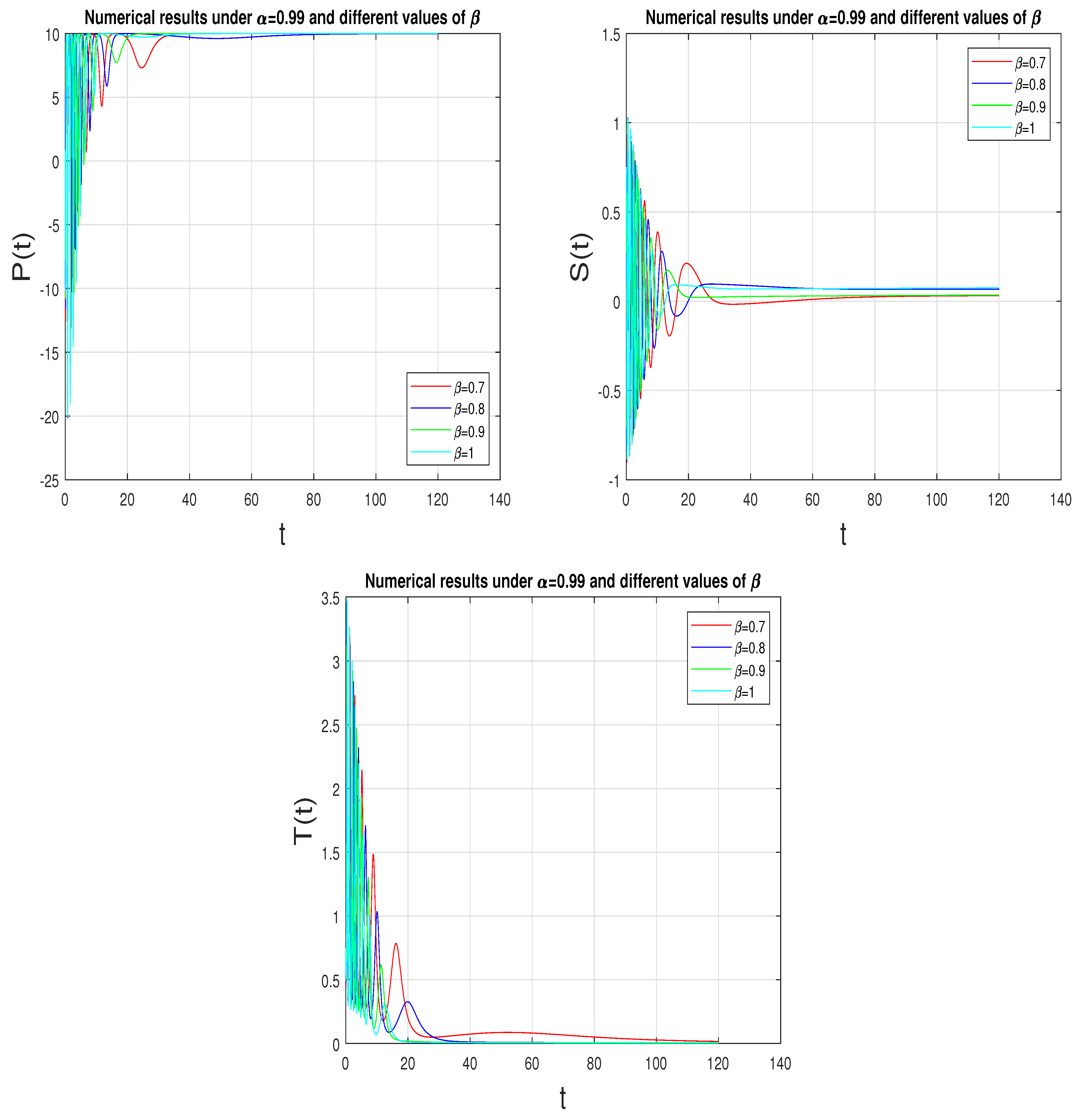
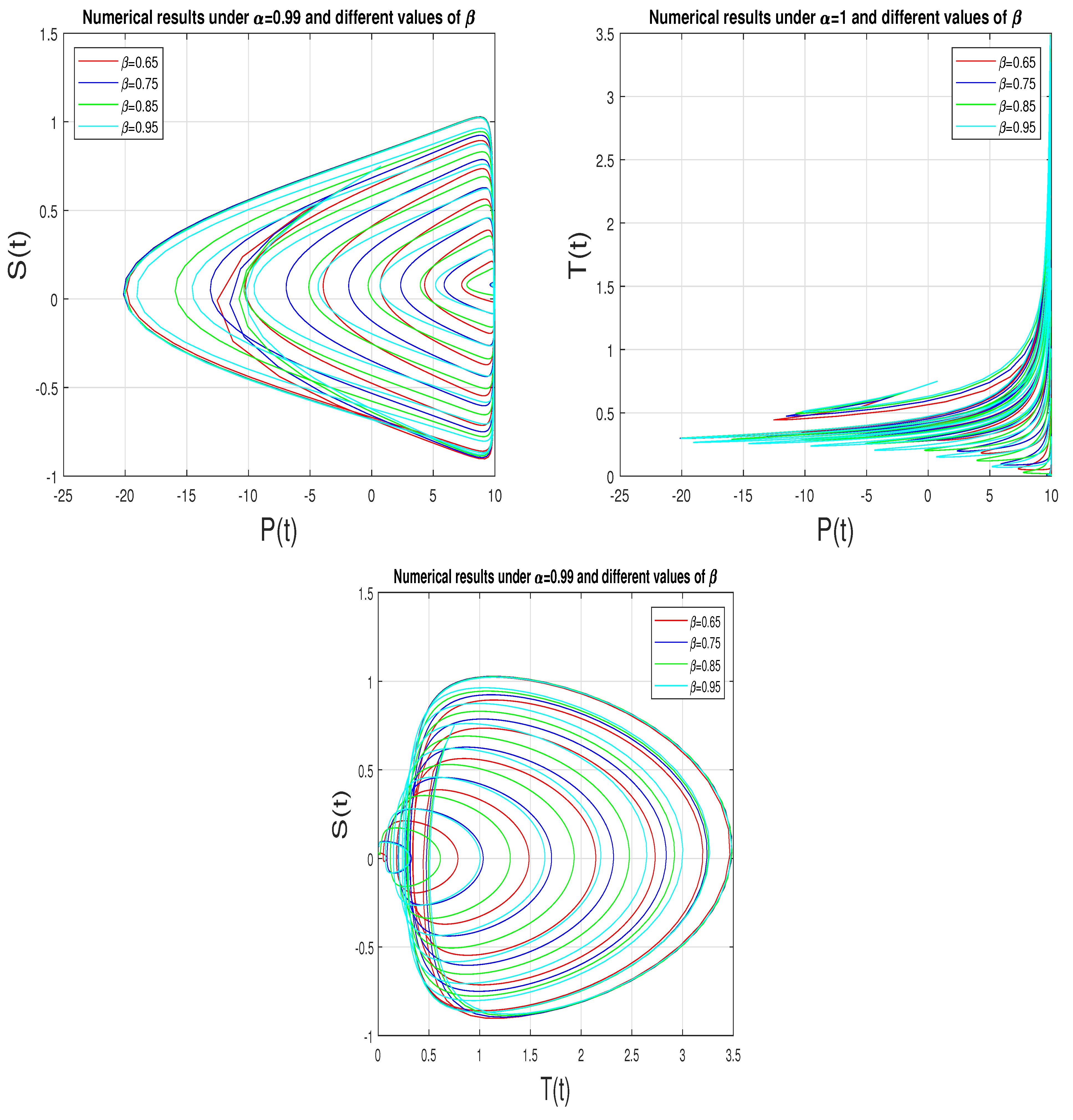
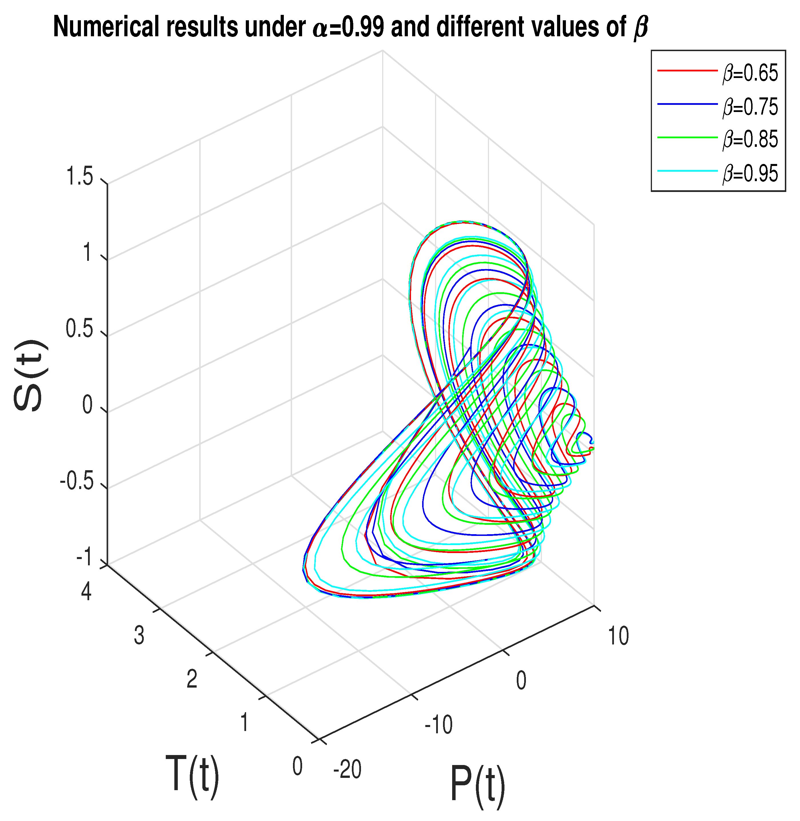
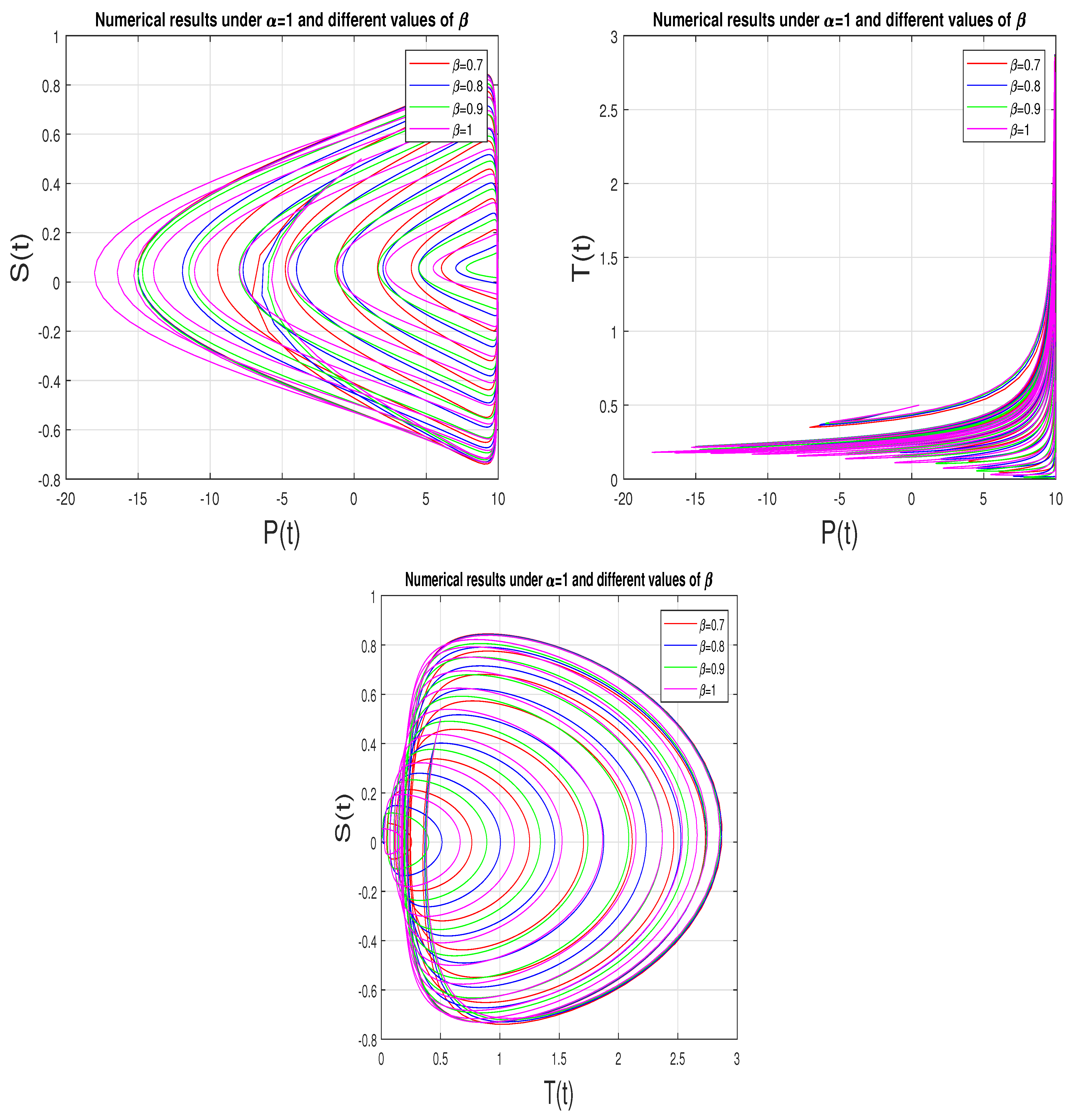
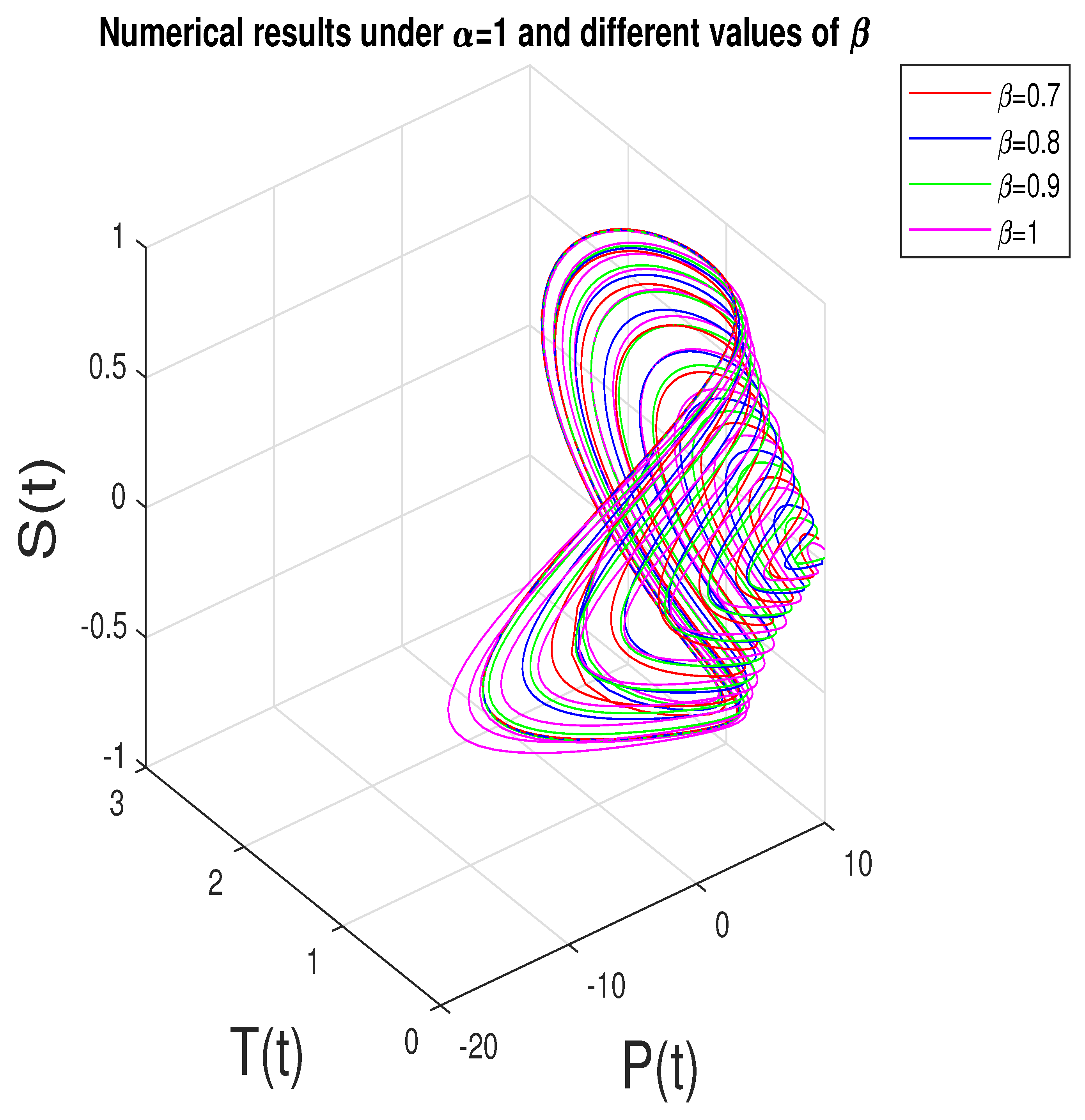
Now, we are going to show the application of the derived numerical scheme in Section 4. We consider two cases containing different fractal, fractional, and initial conditions (ICs) to achieve this aim. The parameters of the studied model are chosen as $A=2,B=25$ and $C=10$. For the first case we consider $P\left(0\right)=1,T\left(0\right)=1$ and $S\left(0\right)=1$(t) and $\beta =0.7,0.8,0.9$ and $\beta =1$ are selected as the fractal orders. In this case, we consider $\alpha =0.99$ as the fractional order. Figures related to this case can be found in Figure 1, Figure 2 and Figure 3. Figure 1 shows the approximate solutions of the state variables. 2D diagrams showing the numerical results can be seen in Figure 3. Furthermore, the chaotic behaviour of the approximate results can be observed in Figure 3.

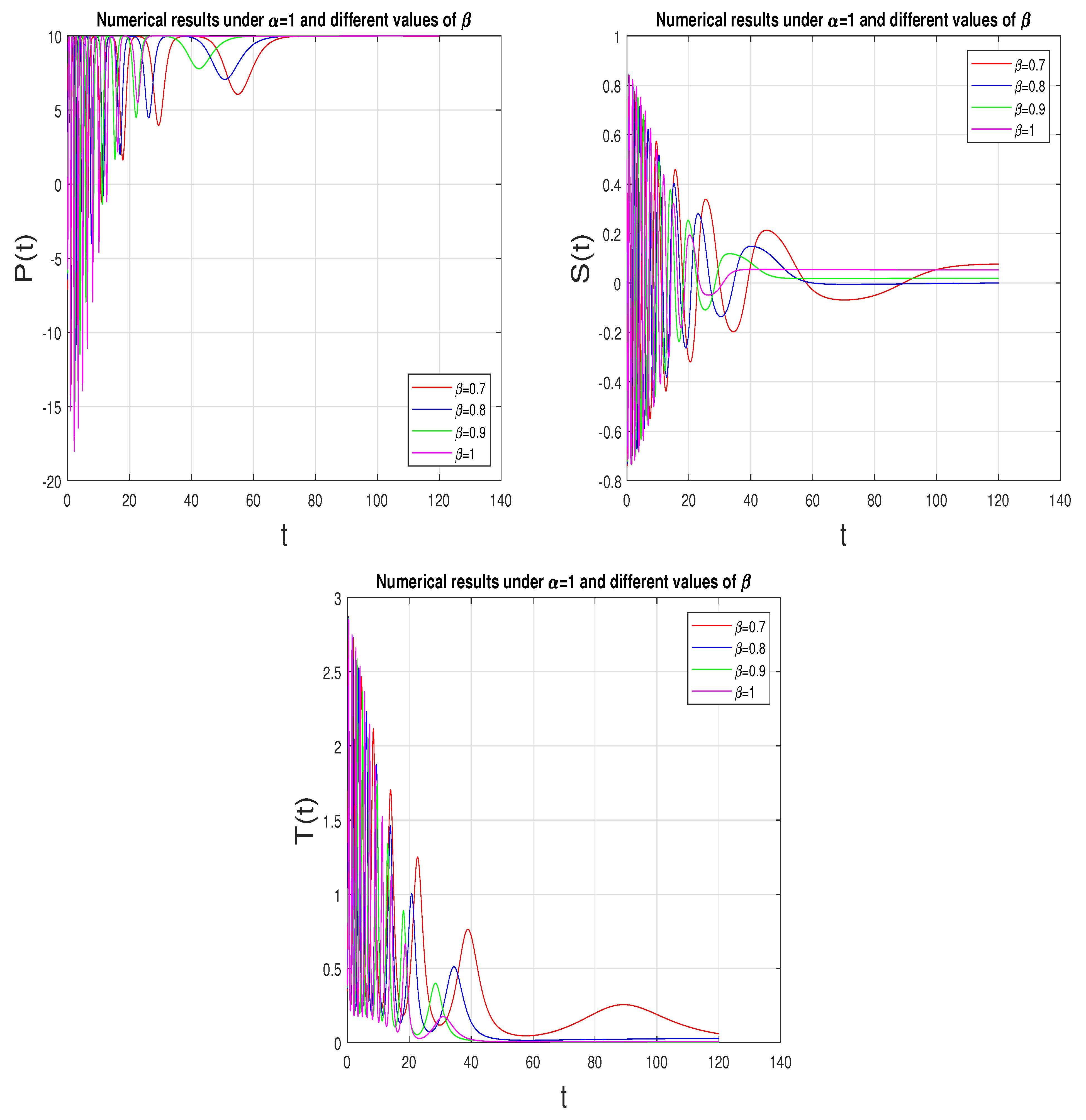
For the second case, we hold $A=1.5,B=18,C=10,P\left(0\right)=1,T\left(0\right)=1$ and $S\left(0\right)=1$ and $\beta =0.65,0.75,0.85$ and $\beta =0.95$ are picked as the fractal orders. We take $\alpha =1$ as the fractional order to see how the behaviours of numerical solutions change. Similar to the first case, Figures reporting the numerical results are shown in Figure 4, Figure 5 and Figure 6. Figure 4 is responsible to reveal the approximate results of the state variables under the chosen initial conditions. 2D diagrams displaying the results can be viewed in Figure 5. Furthermore, the chaotic performance of the approximate results can be seen in Figure 6. The provided Figures reveals the changes which have occurred by altering the fractal–fractional orders and initial conditions.

6. Conclusions

During this study, we designed the fractal–fractional order model of the the circumscribed self-excited spherical attractor by employing an ABC fractal–fractional operator. Furthermore, Schauder’s and Banach’s fixed-point theorems were applied to display the existence of solutions for the suggested dynamical system. We discovered the solutions of Ulam–Hyres stability for the system using nonlinear functional analysis. Moreover, to obtain the approximate solutions of the considered problem and to see how the solutions behave, we employed the effective algorithm under various amounts of fractal and fractional orders. We plotted the graphs of solutions for each case to show how the results change under different conditions.

References

- Kengne, J.; Negou, A.N.; Tchiotsop, D. Antimonotonicity, chaos and multiple attractors in a novel autonomous memristor-based jerk circuit. Nonlinear Dyn. 2017, 88, 2589–2608. [Google Scholar] [CrossRef]
- Sprott, J.C. Some simple chaotic flows. Phys. Rev. E 1994, 50, R647–R650. [Google Scholar] [CrossRef] [PubMed]
- Ghosh, D.; Chowdhury, A.R.; Saha, P. Multiple delay Rossler system-Bifurcation and chaos control. Chaos Solitons Fractals 2008, 35, 472–485. [Google Scholar] [CrossRef]
- Anwar, M.S.; Sar, G.K.; Ray, A.; Ghosh, D. Behavioral study of a new chaotic system. Eur. J. Spec. Top. 2020, 229, 1343–1350. [Google Scholar] [CrossRef]
- Ray, A.; Ghosh, D. Another new chaotic system: Bifurcation and chaos control. Int. J. Bifurc. Chaos 2020, 30, 2050161. [Google Scholar] [CrossRef]
- Bao, H.; Hua, Z.; Wang, N.; Zhu, L.; Chen, M.; Bao, B. Initials-boosted coexisting chaos in a 2-D sine map and its hardware implementation. IEEE Trans. Ind. 2020, 17, 1132–1140. [Google Scholar] [CrossRef]
- Bao, B.; Zhu, Y.; Li, C.; Bao, H.; Xu, Q. Global multistability and analog circuit implementation of an adapting synapsebased neuron model. Nonlinear Dyn. 2020, 101, 1105–1118. [Google Scholar] [CrossRef]
- Ray, A.; Ghosh, D.; Chowdhury, A.R. Topological study of multiple coexisting attractors in a nonlinear system. Phys. Math. Theor. 2009, 42, 385102. [Google Scholar] [CrossRef]
- Bayani, A.; Rajagopal, K.; Khalaf, A.J.M.; Jafari, S.; Leutcho, G.D.; Kengne, J. Dynamical analysis of a new multistable chaotic system with hidden attractor: Antimonotonicity, coexisting multiple attractors, and offset boosting. Phys. Lett. A 2019, 383, 1450–1456. [Google Scholar] [CrossRef]
- Sprott, J.C.; Jafari, S.; Khalaf, A.J.M.; Kapitaniak, T. Megastability: Coexistence of a countable infinity of nested attractors in a periodically-forced oscillator with spatiallyperiodic damping. Eur. Phys. J. Spec. 2017, 226, 1979–1985. [Google Scholar] [CrossRef] [Green Version]
- Leutcho, G.D.; Khalaf, A.J.M. A new oscillator with mega-stability and its Hamilton energy: Infinite coexisting hidden and self-excited attractors. Chaos Interdiscip. J. Nonlinear Sci. 2020, 30, 033112. [Google Scholar] [CrossRef] [PubMed]
- Leutcho, G.D.; Jafari, S.; Hamarash, I.I.; Kengne, J.; Njitacke, Z.T.; Hussain, I. A new megastable nonlinear oscillator with infinite attractors. Chaos Solitons Fractals 2020, 134, 109703. [Google Scholar] [CrossRef]
- Zhang, Y.; Liu, Z.; Wu, H.; Chen, S.; Bao, B. Two-memristor-based chaotic system and its extreme multistability reconstitution via dimensionality reduction analysis. Chaos Solitons Fractals 2020, 127, 354–363. [Google Scholar] [CrossRef]
- Zhang, Y.; Liu, Z.; Wu, H.; Chen, S.; Bao, B. Extreme multistability in memristive hyper-jerk system and stability mechanism analysis using dimensionality reduction model. Eur. Phys. J. Spec. Top. 2019, 228, 1995–2009. [Google Scholar] [CrossRef]
- Li, H.; Bao, H.; Zhu, L.; Bao, B.; Chen, M. Extreme multistability in simple area-preserving map. IEEE Access 2020, 8, 175972–175980. [Google Scholar] [CrossRef]
- Li, C.; Sprott, J.C. Variable-boostable chaotic flows. Optik 2016, 127, 10389–10398. [Google Scholar] [CrossRef]
- Pham, V.T.; Akgül, A.; Volos, C.; Jafari, S.; Kapitaniak, T. Dynamics and circuit realization of a no-equilibrium chaotic system with a boostable variable. AEU Int. J. Electron. Commun. 2017, 78, 134–140. [Google Scholar] [CrossRef]
- Touchent, K.A.; Hammouch, Z.; Mekkaoui, T. A modified invariant subspace method for solving partial differential equations with non-singular kernel fractional derivatives. Appl. Math. Nonlinear Sci. 2020, 5, 35–48. [Google Scholar] [CrossRef]
- Rashid, S.; Hammouch, Z.; Kalsoom, H.; Ashraf, R.; Chu, Y.M. New investigation on the generalized K-fractional integral operators. Front. Phys. 2020, 25. [Google Scholar] [CrossRef]
- Fatmawati, M.A.K.; Bonyah, E.; Hammouch, Z.; Shaiful, E.M. A mathematical model of tuberculosis (TB) transmission with children and adults groups: A fractional model. Aims Math. 2020, 5, 2813–2842. [Google Scholar] [CrossRef]
- Abdeljawad, T.; Rashid, S.; Hammouch, Z.; İşcan, İ.; Chu, Y.M. Some new Simpson-type inequalities for generalized p-convex function on fractal sets with applications. Adv. Differ. Equ. 2020, 1, 1–26. [Google Scholar] [CrossRef]
- Li, Y.; Cang, S.; Kang, Z.; Wang, Z. A new conservative system with isolated invariant tori and six-cluster chaotic flows. Eur. Phys. J. Spec. Top. 2020, 229, 1335–1342. [Google Scholar] [CrossRef]
- Cang, S.; Li, Y.; Xue, W.; Wang, Z.; Chen, Z. Conservative chaos and invariant tori in the modified Sprott A system. Nonlinear Dyn. 2020, 99, 1699–1708. [Google Scholar] [CrossRef]
- Ramamoorthy, R.; Jamal, S.S.; Hussain, I.; Mehrabbeik, M.; Jafari, S.; Rajagopal, K. A New Circumscribed Self-Excited Spherical Strange Attractor. Complexity 2021, 2021, 8068737. [Google Scholar] [CrossRef]
- Farman, M.; Akgül, A.; Abdeljawad, T.; Naik, P.A.; Bukhari, N.; Ahmad, A. Modeling and analysis of fractional order Ebola virus model with Mittag-Leffler kernel. Alex. Eng. J. 2022, 61, 2062–2073. [Google Scholar] [CrossRef]
- Partohaghighi, M.; Akgül, A. Modelling and simulations of the SEIR and Blood Coagulation systems using Atangana-Baleanu-Caputo derivative. Chaos Solitons Fractals 2021, 150, 111135. [Google Scholar] [CrossRef]
- Farman, M.; Akgül, A.; Askar, S.; Botmart, T.; Ahmad, A.; Ahmad, H. Modeling and analysis of fractional order Zika model. AIMS Math. 2021, 3, 4. [Google Scholar] [CrossRef]
- Aslam, M.; Farman, M.; Ahmad, H.; Gia, T.N.; Ahmad, A.; Askar, S. Fractal fractional derivative on chemistry kinetics hires problem. AIMS Math. 2021, 7, 1155–1184. [Google Scholar] [CrossRef]
- Singh, R.; Abdeljawad, T.; Okyere, E.; Guran, L. Modeling, analysis and numerical solution to malaria fractional model with temporary immunity and relapse. Adv. Differ. Equ. 2021, 1, 1–27. [Google Scholar]
- Khan, H.; Begum, R.; Abdeljawad, T.; Khashan, M.M. A numerical and analytical study of SE (Is)(Ih) AR epidemic fractional order COVID-19 model. Adv. Differ. Equ. 2021, 1, 1–31. [Google Scholar] [CrossRef]
- Akgül, E.K.; Akgül, A.; Yavuz, M. New illustrative applications of integral transforms to financial models with different fractional derivatives. Chaos Solitons Fractals 2021, 146, 110877. [Google Scholar] [CrossRef]
- Özköse, F.; Yılmaz, S.; Yavuz, M.; Öztürk, İ.; Şenel, M.T.; Bağcı, B.Ş.; Doğan, M.; Önal, Ö. A Fractional Modeling of Tumor–Immune System Interaction Related to Lung Cancer with Real Data. Eur. Phys. J. Plus 2022, 137, 1–28. [Google Scholar] [CrossRef]
- Phuong, N.D.; Sakar, F.M.; Etemad, S. Rezapour, S. A novel fractional structure of a multi-order quantum multi-integro-differential problem. Adv. Differ. Equ. 2020, 633, 1–23. [Google Scholar]
- Mohammadi, H.; Kumar, S.; Rezapour, S.; Etemad, S. A theoretical study of the Caputo–Fabrizio fractional modeling for hearing loss due to Mumps virus with optimal control. Chaos Solitons Fractals 2021, 144, 110668. [Google Scholar] [CrossRef]
- Baleanu, D.; Jajarmi, A.; Asad, J.H.; Blaszczyk, T. The motion of a bead sliding on a wire in fractional sense. Acta Phys. Pol. A 2017, 131, 1561–1564. [Google Scholar] [CrossRef]
- Hammouch, Z.; Yavuz, M.; Özdemir, N. Numerical solutions and synchronization of a variable-order fractional chaotic system. Math. Model. Numer. Simul. 2021, 1, 11–23. [Google Scholar] [CrossRef]
- Özköse, F.; Yavuz, M. Investigation of interactions between COVID-19 and diabetes with hereditary traits using real data: A case study in Turkey. Comput. Biol. Med. 2021, 141, 105044. [Google Scholar] [CrossRef]
- Veeresha, P.; Yavuz, M.; Baishya, C. A computational approach for shallow water forced Korteweg–De Vries equation on critical flow over a hole with three fractional operators. Int. J. Optim. Control. Theor. Appl. (IJOCTA) 2021, 11, 52–67. [Google Scholar] [CrossRef]
- Baleanu, D.; Sajjadi, S.S.; Asad, J.H.; Jajarmi, A.; Estiri, E. Hyperchaotic behaviours, optimal control, and synchronization of a nonautonomous cardiac conduction system. Adv. Differ. Equ. 2021, 157, 1–24. [Google Scholar]
- Guariglia, E. Riemann zeta fractional derivative—Functional equation and link with primes. Adv. Differ. Equ. 2019, 1, 261. [Google Scholar] [CrossRef]
- Chen, Y.; Yan, Y.; Zhang, K. On the local fractional derivative. J. Math. Anal. Appl. 2010, 362, 17–33. [Google Scholar] [CrossRef] [Green Version]
- Ortigueira, M.D.; Coito, F. From differences to derivatives. Fract. Calc. Appl. Anal. 2004, 7, 459–471. [Google Scholar]
- Chalice, D.R. A characterization of the Cantor function. Am. Math. Mon. 1991, 98, 255–258. [Google Scholar] [CrossRef]
- Li, C.; Dao, X.; Guo, P. Fractional derivatives in complex planes. Nonlinear Anal. 2009, 71, 1857–1869. [Google Scholar] [CrossRef]
- He, J.H. A Tutorial Review on Fractal Spacetime and Fractional Calculus. Int. J. Theor. Phys. 2014, 53, 3698–3718. [Google Scholar] [CrossRef]
- Atangana, A. Fractal-fractional differentiation and integration: Connecting fractal calculus and fractional calculus to predict complex, system. Chaos Solitons Fractals 2017, 102, 396–406. [Google Scholar] [CrossRef]
- Atangana, A.; Akgül, A.; M, K. Owolabi, Analysis of fractal fractional differential equations. Alex. Eng. J. 2021, 59, 1117–1134. [Google Scholar] [CrossRef]
- Owolabi, K.M.; Atangana, A.; Akgül, A. Modelling and analysis of fractal-fractional partial differential equations: Application to reaction-diffusion model. Alex. Eng. J. 2020, 59, 2477–2490. [Google Scholar] [CrossRef]
- Heydari, M.H.; Razzaghi, M.; Avazzadeh, Z. Orthonormal Bernoulli polynomials for space–time fractal-fractional modified Benjamin–Bona–Mahony type equations. Eng. Comput. 2021, 1–14. [Google Scholar] [CrossRef]
Figure 1.
Numerical solutions under different values of the fractal order .
Figure 2.
2D solutions under different values of the fractal order .
Figure 3.
3D solutions under different values of the fractal order .
Figure 4.
Figure 5.
Figure 6.
Publisher’s Note: MDPI stays neutral with regard to jurisdictional claims in published maps and institutional affiliations. |
© 2022 by the authors. Licensee MDPI, Basel, Switzerland. This article is an open access article distributed under the terms and conditions of the Creative Commons Attribution (CC BY) license (https://creativecommons.org/licenses/by/4.0/).
Share and Cite
MDPI and ACS Style
Partohaghighi, M.; Akgül, A.; Alqahtani, R.T. New Type Modelling of the Circumscribed Self-Excited Spherical Attractor. Mathematics 2022, 10, 732. https://0-doi-org.brum.beds.ac.uk/10.3390/math10050732
AMA Style
Partohaghighi M, Akgül A, Alqahtani RT. New Type Modelling of the Circumscribed Self-Excited Spherical Attractor. Mathematics. 2022; 10(5):732. https://0-doi-org.brum.beds.ac.uk/10.3390/math10050732
Chicago/Turabian StylePartohaghighi, Mohammad, Ali Akgül, and Rubayyi T. Alqahtani. 2022. "New Type Modelling of the Circumscribed Self-Excited Spherical Attractor" Mathematics 10, no. 5: 732. https://0-doi-org.brum.beds.ac.uk/10.3390/math10050732
Note that from the first issue of 2016, this journal uses article numbers instead of page numbers. See further details here.