
Statistical Methods with Applications in Data Mining: A Review of the Most Recent Works


1
CMUP, Departamento de Matemática, Faculdade de Ciências, Universidade do Porto, rua do Campo Alegre s/n, 4169-007 Porto, Portugal
2
Departamento de Matemática, Faculdade de Ciências, Universidade do Porto, rua do Campo Alegre s/n, 4169-007 Porto, Portugal
*
Author to whom correspondence should be addressed.
†
These authors contributed equally to this work.
Mathematics 2022, 10(6), 993; https://0-doi-org.brum.beds.ac.uk/10.3390/math10060993
Submission received: 21 February 2022
/
Revised: 11 March 2022
/
Accepted: 17 March 2022
/
Published: 19 March 2022
(This article belongs to the Special Issue Statistical Methods in Data Mining)
Abstract
:The importance of statistical methods in finding patterns and trends in otherwise unstructured and complex large sets of data has grown over the past decade, as the amount of data produced keeps growing exponentially and knowledge obtained from understanding data allows to make quick and informed decisions that save time and provide a competitive advantage. For this reason, we have seen considerable advances over the past few years in statistical methods in data mining. This paper is a comprehensive and systematic review of these recent developments in the area of data mining.
Keywords:
data mining; state of the art; statistical methods; machine learning; statistical learning; deep learningMSC:
62J07; 62H30; 68T10; 68T071. Introduction
Data mining (DM) is the process of finding patterns and correlations within large data sets to predict outcomes. Through techniques that range from statistics to machine learning or to artificial intelligence, DM has entered all areas of knowledge by allowing us to make informed decisions based on the the data themselves.
In this review, we will provide the state of the art in statistical methods in DM, by considering the most cited papers in the most impactful journals over the period spanning mainly from 2020 to the present, 2022.
Given the vast range of topics that DM covers, it is not possible to have a strict procedure regarding the choice of papers. Statistics journals and computer science journals differ substantially in the way articles are shared and have their success and impact measured. Given this impossibility for an absolute procedure, each subsection has the most relevant recently published papers in the area.
In the special issue of Statistical Methods in Data Mining https://0-www-mdpi-com.brum.beds.ac.uk/journal/mathematics/special_issues/Statistical_Methods_Data_Mining (accessed on 20 February 2022),
“Statistics is, nowadays, more important than ever because of the availability of large amounts of data in many domains like science, finance, engineering, medicine, etc. For a long time, statistics has developed as a sub-discipline of mathematics. Nevertheless, computing is also a very important tool for statistics. This is particularly true in statistical methods in data mining, which is an interdisciplinary field involving the analysis of large existing databases in order to discover patterns and relationships in the data. It differs from traditional statistics on the size of the dataset and on the fact that the data were not initially collected according to some experimental design but rather for other purposes. On the other hand, asymptotic analysis, which has for a long time been an important area of statistics approaching problems where the sample size (and more recently, also, the number of variables) tends to infinity, is obviously also appropriate in data mining for dealing with huge amounts of data.”
In the next sections, we will discuss the problem of statistical significance (the famous p-value), which is very relevant in the presence of large number of tests; then, we discuss high-dimensional data, including LASSO, RIDGE, PCA, and other topics. Other recent topics in regression will follow and then other recent developments in supervised classification methods. Although all of these topics can be cast in the area of statistical learning, we consider next a new section devoted to other recent developments in statistical learning. We proceed with a more extensive section of neural networks and deep learning, including applications in computer vision, time series and other sequence data, dimensionality reduction, density estimation, etc. The last three sections are devoted to clustering, software applications and closing remarks.
2. Statistical Significance
We will start by briefly discussing recent views on the topic of statistical significance—the claim that a result of an experiment is not likely to occur randomly or by chance, but is instead likely to be attributable to a specific cause. Many areas of knowledge that depend on data analysis and research, such as physics, medicine or economics, need this metric as a way to evaluate the accuracy of the conclusions.
The most broadly accepted metric in the science community is the p-value; results that have a p-value smaller than the threshold (usually 0.05) are said to be statistically significant, while the rest are branded as inconclusive. The drawbacks of this classification are well known [1] and recently, there has been a pull against this binary classification, as many studies are labeled contradictory and much research goes to waste [2]. A group of authors in [3] proposed tightening the p threshold to 0.005. In [4], the authors go further by proposing to abandon completely the absolute screening role of statistical significance. They instead propose to treat the p-value as a continuous metric, which, helped by the other metrics—e.g., data quality, related prior evidence, plausibility of mechanism, study design, and other factors that vary by research domain—leads to a more complete decision on the study in question.
A related fundamental question in statistical significance is whether two means differ or not. For this, the most popular approach is the t-test, which has a primary role in many of the empirical sciences. In recent years, several different Bayesian t-tests have been introduced due to their theoretical and practical advantages. In [5], a flexible t-prior for standardized effect size is proposed that gives the possibility to compute the Bayes factor by evaluating a single numerical integral. It generalizes prior work, with the previous objective and subjective t-test Bayes factors as special cases.
Another relevant question in the area regards ways to combine individual p-values to aggregate multiple small effects. In order to overcome computational issues that performing this operations with the traditional methods in large and complex data sets provoke, in [6], the authors propose a new test that is defined as a weighted sum of Cauchy transformation of the individual p-values. They show that this new test is not only accurate, but also equally as simple to perform as the classic t-test or z-test.
When performing model selection, often, different criteria used reach different conclusions, and justification of their use and why they were chosen is often lacking in research papers. In [7], the case of information criteria (ICs) based on penalized likelihood is analyzed, and a different view on these criteria that can help in interpreting their practical implications in more complex situations in order to make informed decisions is presented.
3. High-Dimensional Data
In this section, we discuss the case when the number of features p is much larger than the number of observations N, . Data in this category suffer from the aforementioned curse of dimensionality: computational burden, statistical inaccuracy and algorithmic instability. An overview of methods in high-dimensional data can be found in [8]. In this section, we consider penalized regression and feature selection, feature screening for ultrahigh-dimensional problems, estimation and inversion of covariance matrices and linear discriminant analysis in high dimensions, statistical inference for longitudinal data with ultrahigh-dimensional covariates and a new method of principal component analysis.
In the case of regression, the most common approach consists of using regularization, that is, applying penalties on the size of the regression coefficients, performing feature selection and model fitting simultaneously. In general, given input data and response data , with a Tikhonov regularization term given by , the problem becomes,
For LASSO, we drop the Tikhonov regularization term and use ; for RIDGE regression, we also drop the Tikhonov regularization term and use ; and for Elastic Net, we keep the full formulation with . An equivalent and more common formulation for Elastic Net is:
The LASSO regression has the advantage over RIDGE of not only reducing the size of the coefficients, but also setting several to zero, thus reducing the dimensionality of the data. However, LASSO performs poorly in terms of highly correlated features, tending to choose one of them and ignore the others, and generally selects n features before saturating. To overcome this limitation, Elastic net combines the two approaches. In Figure 1, one can see why LASSO usually sets some of the coefficients to zero, since the point inside the corresponding parameter space closest to the least squares solution is in a corner; that is, the first coordinate equals zero (in the case of the figure). In the case of more dimensions, the number of corners and flat edges is much greater, increasing therefore the possibility of zero coefficients.
One traditional approach to selecting features consists in finding the best subset of the p original features; unfortunately, it is not feasible in practice when p is moderately large. This is also a particular case of formulation (1) if we drop the Tikhonov regularization term and use , and it is known as the sparse regression problem [9] (in fact, is not really a norm). This case has the advantage of sparsifying the regressor without unwanted shrinking, while using the -norm leads to biased regression regressors, penalizing both large and small coefficients.
In [9], a new binary convex reformulation, which is equivalent to (1) with , and a novel cutting plane algorithm that solves to provable optimality exact sparse regression problems are presented, which can deal with regressor dimensions in the 100,000 s, with an improvement of two orders of magnitude over similar known methods, while being faster (faster than LASSO). The results show that exact sparse regression can solve high-dimensional problems, refuting the idea that heuristic methods are necessary (see Table 1 [9]).
When performing a regression model on high-dimensional data, if the data are distributed (meaning, large-scale data, stored in L different local machines), traditional methods discussed above as LASSO are not applicable due to storage and computation limitations. Furthermore, if the data feature heavy-tailed noise, most theories, namely, least squares and Huber loss-based statistics, would not work, as the assumption of a finite variance for the noise is not fulfilled. The common approach to such problems is the averaging divide-and-conquer approach, where one builds, on each machine, a local estimator by solving
where is the set of data indexes from the machine, and is the quantile regression loss function (see Roger Koenker. Quantile Regression. Cambridge University Press, 2005), and then averaging over all machines: . Similar constructed debiased approaches also exist but they all suffer from several problems, namely, being computationally costly and the local estimator being no longer sparse. In [10], the authors propose a new distributed estimator for estimating a high-dimensional linear model with heavy-tailed noise that achieves the same convergence rate as the ideal case with pooled data, while establishing the support recovery guarantee.
For ultrahigh-dimensional problems, the seminal work by Fan and Lv [11] introduces the notion of sure screening and proposes a new method called sure independence screening based on correlation learning in order to reduce dimensionality from high to a moderate scale below the sample size. In [12], the authors also use screening procedures that make some assumptions on the the data. Their approach, which eliminates redundant covariates in high-dimensional data, is a model-free feature screening procedure. The method, known as covariate information number-sure independence screening (CIS), can be used for data with continuous features, with any kind of response. The new method is based on a covariate information number (CIN), which captures the marginal association of each feature with the response, without assuming any specific underlying model, and can be interpreted in terms of the traditional Fisher information in statistics. A first model-free forward screening based on the concept of cumulative divergence is introduced in [13]. Cumulative divergence is a new correlation metric that characterizes functional dependence; it is robust to the presence of outliers in the conditioning variable. In contrast to marginal screening approaches, in this new model, the joint correlations among features are considered, while also being robust to model misspecification.
In statistical methods, we often need to use covariance matrices and their inversion; their calculation can be innacurate, numerically unstable and unfeasible in high-dimensional problems. The authors of [14] establish the first analytic formula for nonlinear shrinkage estimation of covariance matrices. It performs better than previous similar models, being about 1000 times faster, with similar accuracy, when compared with Quantized Eigenvalues Sampling Transform (QuEST), and it is also able to tackle covariance matrices of dimension of an order up to 10,000. Methods such as linear discriminant analysis are heavily dependent on a good estimation of the mean vectors and the population covariance matrix, while being based on the premise of an equal population covariance matrix among all classes. In [15], the authors introduce an improved LDA classifier based on the assumption that the covariance matrices follow a spiked covariance model (see [15] for further details).
In [16], the authors approach the problem of statistical inference for longitudinal data with ultrahigh-dimensional features, by introducing a novel quadratic decorrelated inference function approach. It simultaneously eliminates the effect of unwanted parameters and accounts for the correlation to improve the efficiency of the estimation process. Simulation studies conducted by the authors show that the newly proposed method can control Type I error for testing a low-dimensional parameter of interest and the false discovery rate in the multiple testing problem.
Linear combinations of covariates are a traditional way of reducing dimension, for instance, principal component analysis (PCA), although the components retained have some loss of information which, sometimes, is crucial for other tasks. In [17], the authors introduce a new paradigm which replaces high-dimensional covariates with a small number of linear combinations in the context of regression, which does not cause loss of information. In [18], a new method of PCA, called Tensor Robust Principal Component Analysis (TRPCA), is introduced. It aims to exactly recover the low-rank and sparse components. This same low-rank tensor recovery has applications in many areas, given the amount of high-dimensional data available nowadays, often unlabelled. In [19], the authors analyze the case of visual data, which can be easily corrupted and noisy, and introduce a unified presentation of the surrogate-based formulations that include simultaneously the features of rectification and alignment, and establish error bounds for the recovered tensor.
4. Regression
Regression is one of the oldest areas of data mining that this paper covers, but it is still one of the most active fields of research, given its important and wide uses across fields of science. In this section, we will cover some of these recent developments.
When dealing with big data sets, dividing the data among several machines is a common approach to overcoming hardware limitations. Recently, this divide-and-conquer technique has been adapted in the field of statistics to include inferential procedures, based on the mean and other measures of central tendency. These approaches have some shortcomings, namely, assuming homoscedastic errors or sub-Gaussian tails. In order to tackle these issues, the work in [20] proposes to use quantile regression in order to extract features of the conditional distribution of the response in a two-step model that does not sacrifice accuracy.
The RIDGE formulation discussed in the section on high-dimensional data (Equation (2) with ) attempts to find the best balance between variance and bias by fine-tuning the parameter . However, in practice, the best solution is often setting and finding the minimum-norm solution among those that interpolate the training data. In [21], the authors isolate what appears to be a new phenomenon of implicit regularization for interpolated minimum-norm solutions in Kernel “ridgeless” regression.
The maximum likelihood estimator (MLE), on which methods such as logistic regression rely heavily, has been shown to not always exist. In particular, the MLE does not exist if and only if there is no overlap of data points, i.e., there is a hyperplane separating the data classes in logistic regression. Working on this, the authors of [22] establish the existence of a phase transition in the logistic model with Gaussian features, and compute the phase transition boundary explicitly (see [23] for an R package, mlt, that implements maximum likelihood estimation in the class of conditional transformation models).
In [24], the authors propose a new framework that allows to approximate the eigendecomposition using only the eigendecomposition of the Laplacian and the spectral density of the covariance function. The method allows for theoretical analysis of the error caused by the truncation of the series and the boundary effects. This has vast applications in diverse areas, e.g., medical imaging.
When dealing with strong prior information and weak data, it may happen that the fitted variance is higher than the total variance; in this case, the proportion of variance explained, , can be greater than one, which is a problem. In [25], the authors propose a generalization that has a Bayesian interpretation as a variance decomposition, by suggesting the alternative definition of the variance of the predicted values divided by the variance of predicted values plus the expected variance of the errors.
In [26], the authors reformulate the modal regression problem from a statistical learning viewpoint, which renders the problem dimension-independent.
Although modern massive and high-dimensional data promise the discovery of subtle patterns that might not be possible with a small dataset, they also bring great challenges both computational and statistical. Significant progress has been made in this century in obtaining useful information from large datasets with high-dimensional covariates and sub-Gaussian tails. However, sub-Gaussian tails are not a valid assumption in many practical applications; in fact, heavy-tailed distributions and outliers are a common presence for high-dimensional data. In 1973, Peter Huber introduced the concept of robust regression, which is not as affected by some violations of the linear model assumptions as the traditional least squares model is, for instance, in the presence of outliers and heavy-tailed distributions. However, the robustification parameter is set fixed in the works about robust regression, and this introduces problems of estimation when the sample distribution is not symmetric. In [27], an adaptive Huber regression for robust estimation and inference is proposed where the robustification parameter adapts to the sample size, dimension and moments for optimal balance between bias and robustness. Their methodology, which is extended to allow both heavy-tailed predictors and observation noise, is shown to be more robust and predictive in a real-life application.
In [28], a new method, SuSiE, is introduced for variable selection in linear regression. It focuses on quantifying uncertainty in which variables should be selected. For this, the sparse vector of regression coefficients are written as a sum of ‘single-effect’ vectors, each with one non-zero element. Additionally, a Bayesian analogue of stepwise selection (IBSS) is introduced, which, instead of selecting a single variable at each step, computes a distribution on variables to capture uncertainty regarding which variable to select. Their method is very appropriate in the presence of highly correlated and sparse variables, such as in genetic fine mapping applications, which they illustrate. In [28], the possibility of applying these methods to generic variable-selection problems is also discussed.
5. Other Recent Developments in Supervised Classification Methods
We will now describe some recent developments in other supervised classification methods, such as decision trees, support-vector machines, K-NN, etc.
The oldest method of supervised classification is linear discriminant analysis (LDA) of Fisher (1936) for two classes, and Rao (1948) for more than two. Somewhat similar to PCA, LDA projects the data into a space of a lower dimension (); however, unlike PCA, which finds the space where the data have maximum dispersion, LDA finds the space where the classes are well separated and then, in the prediction phase, for a new query, it chooses the class whose projected mean is the closest. In [29], by using the connection that naturally exists between LDA and linear regression, a penalized LDA is introduced, called the moderately clipped LASSO (MCL), which can be applied when the number of variables is larger than the sample size. In numerical studies, the authors find that it has better finite sample performance than LASSO.
On the topic of linear boundaries, when the data can be perfectly separated by a hyperplane, the support-vector machine (SVM) finds the hyperplane that maximizes the margin between the classes, which is different from the LDA hyperplane. Statistical learning theory suggests also that this hyperplane has good generalization properties. It is, of course, rare that the classes be linearly separable and for that reason, SVMs use the Kernel trick, which consists of projecting the data into a space of larger dimension, eventually infinite, hoping that data are linearly separable there. This is achieved without actually needing to define the mapping. Since all we need is an inner product in the final space, a Kernel function is used that corresponds to an inner product. If w is a vector defining the hyperplane that maximizes the margin (), our problem consists of , where are the initial data and corresponds to the projected values of . Of course, even in the larger space, the data might not be linearly separable and for that reason, SVMs use a relaxation, which consists of using slack variables , and the problem becomes
SVMs have been implemented in many research fields, ranging from text classification to face recognition, financial application, etc. Although SVMs have good properties, such as a small number of parameters to estimate, the possibility of finding the global optimum (unlike neural nets) and being fast in predicting (since only the support vectors are used), they take a long time to train, of the order of . For this reason, they are not very popular with very large data sets and there is not much work about them. Recently, in [30], the authors explored support-vector machines in data mining classification algorithms and summarized the research status of various improved methods of SVM. They found a solution for speeding up the SVM algorithm, and concluded that it can be widely used in the context of big data. The performance of SVMs depends highly upon the choice of Kernel functions and their parameters, as well as on the distance used. Many improvements have been made in the last decade to enhance the accuracy of SVM (see [31]), such as twin SVM (TWSVM), which has a computational cost of approximately one-fourth of the SVM. It requires solving two small-size quadratic programming problems in lieu of solving a single large-size one (SVM), in order to find two nonparallel hyperplanes. In [32], a comprehensive review on twin support-vector machines (TWSVM) and twin support-vector regression (TSVR) is given with applications in classification, regression, semi-supervised learning, clustering, and with applications such as Alzheimer’s disease prediction, speaker recognition, text categorization, image denoising, etc.
Many improvements of TWSVM have been proposed by researchers as a result of its favorable performance, especially in cases of handling large datasets.
Decision trees (DT) are a nonparametric supervised learning method used for classification and regression. The objective is to create a model that predicts the value of a target variable by learning simple decision rules inferred from the data features. A tree can be seen as a piecewise constant approximation. It approximates the data via a series of if-then-else decision rules. It facilitates feature importance and data relations analysis, being easy to interpret.
Despite being a simple model to understand, DTs, by themselves, have some drawbacks. Namely, they are unstable to changes in data, often quite inaccurate, and calculations can become quite complex if a right pruning algorithm is not jointly applied.
In [33], generalized random forests are proposed, a method for nonparametric statistical estimation based on random forests (Breiman, 2001). Forests estimate and theoretical results regarding the consistency and confidence intervals exist for such estimates (see [33]). This paper extends Breiman’s random forests into a flexible method for estimating any quantity , not just , and uses their approach to create new methods for nonparametric quantile regression, conditional average partial effect estimation, and heterogeneous treatment effect estimation via instrumental variables. A software implementation is also provided.
Bayesian additive regression trees (BART) provide an alternative to the parametric assumptions of the linear regression model. In [34], extensions of the original BART to new models are introduced for several different data types, in addition to changes to the BART prior to tackling higher dimensions and smooth regression functions. Recent theoretical results regarding BART are also presented and discussed, as well as the application of methods based on BART to causal inference problems. The paper also describes available software and challenges it may face in the future.
Another nonparametric method of supervised classification is the well-known KNN, which, despite coming from the nonparametric estimation of the densities , results in sorting any new query into the most dominant class amongst its K neighbors. In [35], the authors seek estimators for the entropy of a density distribution, which represents the average information content of an observation, and can be seen as a measure of unpredictability of the system. This has applications in many statistical methods, namely, to test goodness of fit and independent component analysis. They use weighted averages of existing estimators based on the k-nearest neighbor distances of a sample of n independent and identically distributed random vectors. They obtain efficient estimators for larger dimensions than the original estimators, as well as confidence intervals for the asymptotically valid entropy.
In practice, when applying regression or classification models, we can have underfitting (large error in both training and testing) or overfitting (low training error and large expected test error). By using regularization techniques, we can address this gap between the training error and the test error in overfitting. The work in [36] introduces a new regularization method for semi-supervised learning that identifies the direction in which the classifier’s behavior is most sensitive. Naturally occurring systems and several studies suggest that a predictor robust against random and local perturbations is effective in semi-supervised learning. For instance, with neural networks, it is possible to improve the general performance by applying random perturbations to each input in order to create artificial input points and encouraging the model to assign similar outputs to the set of artificial inputs derived from the same point (see [36]). It has been found, however, that random noise and random data augmentation often cause the predictor to be very vulnerable to a small perturbation in a specific direction, known as the adversarial direction, for, instance when using and regularization. Adversarial training (Goodfellow et al. 2015) is an attempt to solve this problem that has succeeded in improving generalization performance and made the model robust against adversarial perturbation. Unlike adversarial training, the work in [36] proposes a method that defines the adversarial directions (only “virtually” adversarial, in fact) without label information and can, for this reason, be applied in semi-supervised learning. The application in supervised and semi-supervised learning tasks on many benchmark datasets demonstrates very competitive performance when compared to state-of-the-art methods.
6. Statistical Learning
The concept of statistical learning refers to a set of tools for modeling and understanding complex data sets, and it combines the areas of statistics and machine learning. It covers a wide range of concepts. In this section, those not covered in other sections will be discussed, normally filed under the topic of statistical learning themselves.
Zero-shot learning aims to recognize objects whose instances may not have been seen during training (classifying images where there is a lack of labeled training data). In the past few years, there has been a rapid increase in the number of new zero-shot learning methods that have been proposed. These are due to the many cases where AI needs to adapt to previously unseen data, from self-driving cars to new disease diagnosis, e.g., COVID-19. In [37], the authors present a comprehensive review on the state of the art in the area, comparing all methods and presenting a new data set to perform the testing in order to have common metrics between models.
When the data in a study are corrupted or heavy-tailed, recently introduced median-of-means (MOM)-based procedures have been shown to outperform classical least-squares estimators (e.g., LASSO). MOM estimators partition the data set into k blocks, , of the same cardinality, and then calculate the median of the K empirical means of each block:
Despite their advantages, these procedures cannot be implemented. In [38], the authors introduce min–max MOM estimators and demonstrate that, both in small and high-dimensional statistics, they obtain similar sub-Gaussian deviation bounds as the alternatives models, while being efficient under moment assumptions on data that may have been corrupted by a few outliers.
In many areas of knowledge, nonparametric estimation of a probability density function is an essential tool in the analysis. Using local polynomial techniques, in [39], the authors introduce a novel nonparametric estimator of a density function. The distinctive feature of this estimator is that it adapts to the boundaries of the support of the density automatically; it does not require particular data modifications or choosing additional tuning parameters, something almost all state-of-the-art methods are incapable of performing without compromising the finite and large-sample properties of the estimator.
Many of the new methods cited in this paper—namely, neural nets, deep learning, boosting, support-vector machines, random forests—have became widely popular and are widely used in all kinds of data sets due to their well-known advantages. In [40], the author compares these new ‘trends’ with the classic approaches, such as ordinary least squares and logistic regression, focusing on the differences between prediction and estimation or prediction and attribution (significance testing).
Given the increasing size and complex structure of data sets in the most varied areas, black-box supervised learning models, such as neural networks, boosted trees, random forests, k-nearest neighbors or support-vector regression, commonly replace more transparent linear and logistic regression models in order to capture nonlinear phenomena. They are, however, difficult to interpret in terms of fully understanding the effects of the features on the response. In many cases, this relationship is vital information. Generally, the solution is to use partial dependence (PD) plots. However, they can produce poor results if the covariates are strongly correlated, as they require extrapolation of the response at predictor values that are significantly outside the multivariate envelope of the training data. To resolve this, in [41], the authors present a new visualization approach called accumulated local effects (ALE) plots, which, in addition to being computationally less expensive, does not require this unreliable extrapolation with correlated features.
In [42], the authors review and introduce a general framework on the area of metaresearch. Metaresearch is the area of research that studies research itself, in order to investigate quality, bias and efficiency. Work in this area is important in maintaining the credibility of the scientific method.
A concept we are all familiar with (even if unknowingly) is prediction-based decision making. It has made its way to government policy decisions, environmental discussions or industry standards. Decisions based on predictions of an outcome have become the norm. This newly acquired attention has been related to how consequential predictive models may be biased, in aspects such as race, gender or class. Studying and correcting such biases has motivated a field of research known as algorithmic fairness. The work in [43] provides a framework for this scattered topic, establishing terminology, notation and definitions, offering a concise reference frame for thinking through the choices, assumptions, and fairness considerations of prediction-based decision making.
In social sciences, structural equation modeling (SEM)—which explains the relationships between measured variables and latent variables, as well as the relationships between latent variables themselves—has become the standard. Recently, however, partial least squares path modeling (PLS-PM), a composite-based approach to SEM, has been gaining traction in a wide range of uses, as it allows researchers to estimate complex models with many constructs and indicator variables, even at low sample sizes. In [44], the authors explore whether, and when, the in-sample measures such as the model selection criteria can substitute out-of-sample criteria that require a holdout sample.
MCMC methods are a fundamental tool for Bayesian inference and they use the Metropolis–Hastings (MH) algorithm ([45,46]), which is used to produce samples from distributions that may otherwise be difficult to sample from, and is generally used for sampling from multidimensional distributions, especially when the number of dimensions is large. Yet, when faced with big data, these methods do not work well. In [47], a new family of Monte Carlo methods is introduced, which is based upon a multidimensional version of the Zig-Zag process in [48]. This new method has often more favorable convergence properties. A sub-sampling version of the Zig-Zag process is introduced, which seems to work well with big data.
Low-rank matrix estimation, which is used in mathematical modeling and data compression, consists of finding an approximating matrix to a given data matrix, and is related to PCA, factor analysis, etc. Many of these estimators are NP-hard but, fortunately, some computationally efficient algorithms using leading eigenvectors exist. The authors of [49] investigate the behavior of eigenvectors for a large class of random matrices whose expectations are low-rank.
In many large-scale regression problems, matrix products such as are needed and in [50], a new and considerably more efficient way to compute is presented. Starting from discretized covariates, these new algorithms manage to be more efficient than previous algorithms, thereby substantially reducing the computational burden for large data sets.
In [51], the authors introduce an alternative procedure to the minimum covariance determinant (MCD) approach. MCD estimates the location and scatter matrix using the subset of a given size with the lowest sample covariance determinant; this is useful, for instance, to avoid outliers. However, the MCD approach cannot be applied when the dimension of the data, p, exceeds the subset size, h. In [51], the authors introduce the minimum regularized covariance determinant (MRCD) approach. It can be applied when , and it differs from the MCD in that the scatter matrix is a convex combination of a target matrix and the sample covariance matrix of the subset. The aim is to substitute the subset-based covariance with a regularized covariance estimate, defined as a weighted average of the sample covariance of the h-subset and a predetermined positive definite target matrix. This estimated covariance matrix is guaranteed to be invertible, it performs in higher dimensions, it is suitable for computing robust distances and for linear discriminant analysis and graphical modeling.
In machine learning and statistics, it is most common to have data which consist of vectors of features. However, in the era of big data, other types of data exist, such as graph recommender systems (users and products with transactions and rating relations), ontologies (concepts with relations), computational biology (protein–protein interactions), computational finance (web of companies with competitor, customer, subsidiary relations, supply chain graph, graph of customer–merchant transactions), etc. (see [52]). It is of course possible to ignore relations and treat these data as vectors of features; however, these relations hold additional valuable information. Most of the research on graphs has been conducted on static graphs (fixed nodes and edges). Many applications, however, involve dynamic graphs that change over time, and in [52], a survey is presented of the recent advances in representation learning for dynamic graphs with several prominent applications and widely used datasets.
7. Neural Networks and Deep Learning
7.1. Introduction
The function obtained by a neural network with input vector , one hidden layer and output is such that
where the parameters b, a and matrices and are to be estimated from data, and the activation functions , are usually the hyperbolic tangent, sigmoid, RELU, etc. (see in Figure 2 a graphical representation of this 1-hidden-layer neural network). Deep networks have many more hidden layers and so, the final function becomes quite difficult to differentiate in order to estimate the parameters, which has to be achieved using some form of gradient descent (GD). Back-propagation was a breakthrough that allowed the training of multilayer networks of neurons and new architectures (SOM, RBF, Hopfield, etc.) and applications appeared. In the 1990s, the use of neural networks was generalized and new developments emerged.
Deep learning or deep neural networks (see Chapter 14 of [53,54] for an overview) has achieved tremendous success in the last decade in many areas such as artificial intelligence, statistics, applied mathematics, clinical research, etc. Deep learning uses many compositions of linear transformations followed by nonlinear ones in order to approximate high-dimensional functions, and it has greatly improved the performance on complex datasets such as images, texts and voices in applications such as computer vision, natural language processing, machine translation, etc. The tremendous success of deep learning is due in part to its response to the bias–variance trade-off, since, by using huge datasets, with millions of samples, the variance is reduced and at the same time, due to the current availability of enormous computing power, one can train large neural networks, which reduces biases. On the other hand, given the huge number of parameters to be estimated, sometimes more parameters than data observations, the training of a deep neural network requires the use of some form of regularization in order to prevent the parameters from ‘exploding’ and avoid overfitting of the model. The regularization consists of adding a penalty to the loss to be optimized, and it results in simpler models. For instance, L2 regularization, or weight decay, is very popular for training neural networks.
On the other hand, L1 regularization introduces sparsity in the weights by forcing some of the weights to be zero, which, in particular, causes some of the features to be discarded. Other forms of regularization exist, such as Dropout (which has some resemblance to bagging introduced by Breiman in 1996 [55]) where during training some number of connections are randomly ignored, with probability p, although during the test, all of the connections are taken into account.
Popular deep learning software use computational graphs, which provide an efficient way of representing function composition and computing gradients by back-propagation. In addition, in order to minimize the total “error” or loss, that is, the average of the errors between the output value given by the network and the real value, for each data observation, another important aspect is the use of stochastic gradient descent (SGD). Thus, in each pass, instead of computing the gradient for the entire dataset, which is computationally very costly, the gradient is only computed for a small random sample. By the law of large numbers, this stochastic gradient should be close to the full-sample one, it converges faster than GD and is widely used in ML. Other important aspects that contribute to the success of deep learning will emerge as we introduce some popular models below.
Despite the huge success of deep learning, one must remember that according to the universal approximation theorem, a neural network with one hidden layer and a linear output layer may approximate any Borel measurable functions well. In practice, a one-hidden-layer neural network with a large number of nodes can still achieve high prediction performance. Taking this into consideration, recently, the authors of [56] introduced a training algorithm, called local linear approximation (LLA), which uses the first-order Taylor expansion to locally approximate activation functions of each neuron, such as RELU, and can be used in both regression and classification problems.
Note that, while any state-of-the-art review always runs the risk of quickly becoming outdated, this section in particular moves fast, and any top method at the time of publishing will likely be surpassed in benchmark tests by the following month. For this reason, the selection of the papers cited on this topic will follow the methods that caused a paradigm shift in the approaches used, as most of the others are combinations and variations on these. This is the case, for instance, in computer vision.
A historical survey on deep learning in neural networks can be found in [57].
7.2. A Statistical View of Deep Learning
In [58], the authors present a survey of recent progress in statistical learning theory, which are useful in deep learning.
According to the authors,
“Broadly interpreted, deep learning can be viewed as a family of highly nonlinear statistical models that are able to encode highly nontrivial representations of data. A prototypical example is a feed-forward neural network with L layers, which is a parameterized family of functions defined on bywhere the parameters are with and , and are fixed non-linearities, called activation functions.”
These authors conclude that, surprisingly, deep learning models find solutions that give a near-perfect fit to noisy training data, and, at the same time, lead to excellent prediction performance on test data; and this is achieved with no explicit effort made to control model complexity.
The classical approach in statistical learning involves a rich, high-dimensional model, combined with some kind of regularization, to encourage simple models, while allowing more complexity if that is warranted by the data. The deep learning models, on the other hand, are built upon two surprising empirical discoveries: (1) As deep learning uses models with many parameters, the fit to the training data is simplified and simple, local optimization approaches, variants of stochastic gradient methods, are extraordinarily successful in finding near-optimal fits to training data. The idea of overparametrization seems contradictory from the point of view of classical learning theory, which states that these models should not generalize well; (2) Deep learning models are, in fact, outside the realms of classical learning theory, they are trained with no explicit regularization and, although they typically overfit the training data, exhibiting a near-perfect fit, with empirical risk close to zero, they produce nonetheless excellent test-prediction performance in a number of settings. They conclude that deep learning practice has demonstrated that poor predictive accuracy is not an inevitable consequence of this benign overfitting.
See the work in [58] for further theoretical details for understanding this behavior of deep learning models and see why, although there is no explicit regularization, implicitly, they impose regularization.
7.3. Examples of Deep Neural Networks
7.3.1. Convolutional Neural Networks (CNN) and Computer Vision
Methods in computer vision have vastly improved in recent years. Object detection—where the goal is to classify individual objects and localize each using a bounding box, and semantic detection/image segmentation—where the task consists of clustering parts of an image together which belong to the same object class, are the two main problems. A performance comparison between all these methods in different benchmark test sets with accompanying papers can be found at https://paperswithcode.com/area/computer-vision (accessed on 20 February 2022), while a review on object detection using deep learning can be found in [59], and a review on image segmentation can be found in [60].
Currently, the vast majority of computer vision algorithms use convolutional neural networks (CNNs). CNNs are a specialized kind of neural network for processing data that has a known grid-like topology. Their uses are diverse, but they are more commonly used on input of the form of image data (2-D).
The idea of using this mathematical concept in computer vision was first introduced by LeCun et al. [61] in 1998, to help solve the problem of recognition of hand-written digits. CNNs are simply neural networks that use convolution in place of matrix multiplication in at least one of their initial layers. This, however, speeds up the learning period immensely as matrix multiplication is computationally costly, and, in these applications, it usually returns a sparse matrix which a CNN can obtain with less redundant information (for more details, see Chapter 9 of [62]).
In Figure 3, we can see the usual configuration of a CNN. In the first stage, the layer performs several convolutions in parallel to produce a set of linear activations. In the second stage, each linear activation is run through a nonlinear activation function, such as the rectified linear activation function (RELU). In the third stage, we use a pooling function to modify the output in order to make it invariant to small translations of the input, while, typically, reducing the size of the data—the most common pooling function is max pooling, which returns the maximum output within a rectangular neighborhood. In the end, the output is flattened into a 1-D array so it can be run through a neural network for classification. The most popular image classification algorithms, including LeNet [61] and AlexNet [63], follow this structure, varying the number of convolutional layers and changing the hyperparameters, such as the pooling width and stride.
While traditional object detectors usually consist of three stages—frame candidate regions on a specified image and locate the object, extract features of these candidate regions, use the trained classifier for classification—current state-of-the-art object detectors either have two stages or only one stage. A two-stage detector is a proposal-driven mechanism, where it initially uses a region proposal network to generate regions of interest (RoIs), and, in the second stage, sends the region proposals down the pipeline for object classification and bounding-box regression. They are the most precise framework, but also slower compared with their counterparts. One of the most successful two-stage detectors is the region-based convolutional neural network (R-CNN) [64], which obtains a manageable number of candidate regions and evaluates convolutional networks independently in each region of interest, by classifying each candidate location as one of the foreground classes or as background. On the other hand, there have also been promising results for one-stage detectors, namely, YOLO [65] and SSD [66], which lose 10–40% to the best two-stage methods in terms of accuracy, but are considerably faster. In [67], the authors present a simple two-stage dense detector named RetinaNet, which matches the speed of previous one-stage detectors, while surpassing the accuracy of all existing state-of-the-art two-stage detectors, including the ones mentioned in this section.
In [68], the authors present a new general framework, called Mask R-CNN, for instance segmentation, which combines elements from the two classic computer vision tasks mentioned before in a simple and efficient way, claiming to surpass all previous methods. Most of the advances in computer vision are driven by powerful baseline systems such as Fast/Faster R-CNN [69,70] and fully convolutional network (FCN) [71] frameworks. Faster R-CNN is built on the R-CNN framework by learning the attention mechanism with a region proposal network (RPN). Building on Faster R-CNN, Mask R-CNN adds a branch for predicting segmentation masks on each region of interest, in parallel with the existing branch for bounding-box regression. That is, to the previous outputs—class label and bounding-box offset—for each candidate object, it adds a third branch that outputs the mask that bounds the object. It improves on previous instance segmentation algorithms, while also excelling at object detection; it is also easily generalized for performing different vision tasks, such as human pose estimation, as the paper shows. Mask R-CNN is simple to train and adds only a small overhead to Faster R-CNN, running at 5 fps.
At the time of publishing, the best-performing model in both object detection and instance segmentation on the COCO test-dev data set is SwinV2-G (HTC++) [72], with 63.1% object AP (average precision) on the former, and 54.4% mask AP on the latter.(see Table 1).
An important challenge in vision tasks is the diversity of the scale of the features we are trying to identify. Convolutional neural networks (CNNs) naturally learn coarse to fine multiscale features through a stack of convolutional operators. This inherent multiscale feature extraction ability of CNNs leads to effective representations for solving numerous vision tasks. Designing a more efficient network architecture is the key to further improving the performance of CNNs. In [73], a new multiscale backbone architecture is introduced, Res2Net, which adds a new dimension, scale, to the previous existing dimensions of depth, width and cardinality.
By exploiting the multiscale potential at a granular level, orthogonal to existing methods that utilize layerwise operations, it can be easily added to previous CNN models, such as ResNet or DLA, improving them further.
A common practice used in convolutional neural networks is flattening a layer followed by a fully connected layer. Despite empirical success, this method discards possible multilinear structures within the data. A solution is proposed in [74]—using tensor algebraic operations, thus preserving this multilinear structure at every layer. The authors propose tensor contraction layers (TCLs)—which reduce the dimensionality of their input while preserving their multilinear structure using tensor contraction—and tensor regression layers (TRLs)—which express outputs through a low-rank multilinear mapping from a high-order activation tensor to an output tensor of arbitrary order—as end-to-end trainable components of neural networks. By replacing fully connected layers with tensor contractions, this method aggregates long-range spatial information while preserving a multimodal structure, while by enforcing a low rank, it reduces the number of parameters needed significantly with minimal impact on accuracy.
Extracting low-rank tensors from data, where unknown deformations and sparse but arbitrary errors exist, is an important problem with many applications across fields. Noise pollution, missing observations, partial occlusion, misalignments and other degradation factors are a common occurrence in visual data, from mobile phones to cameras, surveillance cameras and medical imaging equipment. In [19], a general framework that incorporates the features of rectification and alignment simultaneously, and establishes worst-case error bounds of the recovered tensor, is presented. Previous state-of-the-art methods, such as RASL or TILT, are particular cases of this formulation.
7.3.2. Recurrent Neural Network (RNN) for Time-Series Data and Other Sequential Data
Recurrent neural networks (RNNs) are a class of neural networks that allow previous outputs to be used as inputs while having hidden states. They are naturally suited for processing time-series data and other sequential data, allowing inputs of arbitrary length. They consists of several successive recurrent layers, and these layers are sequentially modeled in order to map the sequence with other sequences. RNNs have a strong capability of capturing the contextual data from a sequence. They are mostly used for natural language processing and speech recognition. RNNs can solve many different kinds of problems and can be categorized into the following: One-to-One—standard mode of classification without RNN (e.g., image classification); Many-to-One—sequence of inputs and a single output (e.g., sentiment analysis); One-to-Many—takes an input and produces a sequence of outputs (e.g., image captioning); Many-to-Many—sequences of inputs and outputs (e.g., text translation); Many-to-Many—sequence-to-sequence learning (e.g., video classification).
RNNs, alone or together with other neural network types, have had uses in the most diverse areas in the past few years. These uses range from enhancing the resolution of images [75] to predicting the price of the stock market [76], predicting the behavior of chaotic systems [77] and detecting process fault [78].
A review on RNNs and long short-term memory (LSTM) networks can be found in [79].
7.3.3. Autoencoders for Dimensionality Reduction and Applications
An autoencoder is a deep neural network that is trained to attempt to copy its input to its output. It is an unsupervised artificial network that efficiently compresses the data from the reduced encoded representation to a representation that is as close to the original input as possible. In doing so, it learns a lower-dimensional representation (encoding) of the higher-dimensional data, capturing the most important parts of the input. Its uses are diverse, from reduction of dimensionality (in fact, principal component analysis is a special case of autoencoding) to anomaly detection and image denoising.
In particular, in recent years, it has been shown to work in character recognition [80], unsupervised image clustering [81], denoising RNA sequences [82], in cybersecurity [83] (see survey of deep-learning methods in cybersecurity in [84]), in 3-D MRI brain segmentation [85], fault diagnosis [86] and unsupervised anomaly detection in high-energy physics [87].
7.3.4. Generative Adversarial Networks (GANs) for Density Estimation and Applications
In classical density estimators, the density function is defined in relatively low dimensions. A generative adversarial network [88], on the other hand, is an implicit density estimator in much higher dimensions, such as data from images, natural scenarios or handwritten data. GANs place a greater emphasis on sampling from the distribution rather than estimation, and define the density implicitly through a source distribution and a generator function , which is usually a deep neural network [53].
GANs use an unsupervised algorithm that discovers and learns regularities and patterns in input data in such a way that it can be used to generate new examples that plausibly could have been drawn from the original dataset. It combines two models: a model that generates candidate outputs and a classifier that evaluates whether the data created by the first model are real or computer-generated. The algorithm ‘fools’ the classifier when half of the input is misclassified. GANs are one of the most cited topics in DL. Their popularity is mostly due to the ability to create photorealistic objects and people or to change settings in a scene [89], but uses of GANs are not limited to image processing. Speech and audio processing, medical information processing and many other areas produce active research in this field.
Recently, due to the outbreak of COVID-19, GANs have been used to improve positive case detection and treatment [90,91]. Other uses include fault diagnosis [92,93] and deraining images (i.e., removing weather effects such as rain or snow from images; [94]). A literature review on the topic can be found in [95], a comparative analysis of Deep Convolutional GAN and Conditional GAN can be found in [96] and a review on progress and research issues in [97].
7.3.5. Other Applications of Deep Learning
Graph neural networks (GNNs) are a class of deep-learning methods designed to perform inference on data described by graphs. A comprehensive survey on GNNs can be found in [98].
Reinforcement learning (RL) concerns an agent interacting with the environment, learning an optimal policy, by trial and error, for sequential decision-making problems. It began with Google DeepMind, becoming popular when it was used to beat the best chess player and the best Go player in the world. Overviews of deep reinforcement learning can be found in [99,100].
Most machine learning methods are built on a common premise: the training and test data are drawn from the same feature space and the same distribution. If this distribution changes, the majority of the models described in this paper have to be rebuilt from scratch, using newly collected training data. It can be expensive or even impossible to collect again the needed training data and rebuild the models in many practical examples. In such cases, knowledge transfer or transfer learning between task domains would be desirable. A network is trained with a large amount of data, with the model learning the weights and bias during training. These weights can be transferred to other networks to test or retrain a similar new model, so that the network can start with pretrained weights instead of training from zero. An overview on the topic can be found in [101] and an application in natural language processing can be found in [102].
Drug design aims to identify (new) molecules with a set of specified properties. Given that it still is a lengthy, expensive, difficult, and inefficient process with a low rate of new therapeutic discovery, there is great interest in developing automated techniques to discover sizable numbers of plausible, diverse and novel candidate molecules with desirable properties. In [103], a novel variational autoencoder for molecular graphs is proposed, whose encoder and decoder are especially designed to account for the unique characteristics of molecular graphs. Experiments reveal that their variational autoencoder can discover plausible, diverse and novel molecules more effectively than several state-of-the-art models.
A new area that has gathered momentum in deep learning is physics-informed neural networks (PINNs)—neural networks that are trained to solve a problem while obeying physical laws (either explicitly or using the system’s symmetries and conservation laws), or to find the physical laws from existing data. Its framework was introduced in [104], and its current state of the art can be found in [105]. This concept of data-driven discovery of governing equations has also seen significant advances recently on the topic of the discovery of coordinates and universal embedding of nonlinear dynamic systems [106,107] (see [108] for a review of Koopman’s theory of nonlinear dynamics).
8. Clustering
In data mining, we are often faced with high-dimensional data where observations have from a few dozen to thousands of features or dimensions. In order to overcome the associated difficulties, such as visualization of the data and the curse of dimensionality (enumeration of all subspaces is prohibitive), a dimensionality reduction technique or feature selection is often employed beforehand. However, the obtained results depend on the dimensionality reduction technique used, many dimensions can be irrelevant to clustering and identifying them is not easy.
Subspace clustering tries to circumvent these problems, by clustering, simultaneously, features and observations. This in turn might result in overlapping clusters in both the space of features and observations. This means that, for instance, it might be possible to identify a cluster of the observations in a subspace with 10% of the dimensions that was not possible to identify in the entire space. There are: (1) Bottom-up approaches which start by finding clusters in low-dimensional spaces and iteratively merge them to find clusters in higher-dimensional spaces; (2) Top-down approaches, which find clusters in the full set of dimensions and then, for each cluster, find the corresponding subspace. In addition, subspace clustering approaches can be categorized into iterative methods, algebraic approaches, statistical methods and spectral clustering-based methods (see [114]).
Subspace clustering has had many successful applications. Recently, novel subspace clustering models have been proposed which use multiple views of the data, not just one, in order to decrease the influence the original features have when the observations are insufficient. These methods produce v subspace representations and feature matrix , corresponding to the optimization problem,
where is a loss function and a regularization term.
As a way to explore the relationships between data points and effectively deal with noise, the work in [114] proposes using a latent representation for multiple views (Latent Multi-view Subspace Clustering). This method learns a latent representation to encode complementary information from multiview features and produces a common subspace representation for all views, rather than one of each individual view. Furthermore, the authors generalize their model for nonlinear correlation, and propose the generalized Latent Multi-view Subspace Clustering (gLMSC). They show by experimenting on both synthetic and benchmark datasets significant advantages of the learned latent representation for multiview subspace clustering when compared to the other modern multiview clustering approaches.
As another illustration and application of the use of multiple views in clustering, in [115], a new method is proposed for detecting coherent groups in crowd scenes.
Other types of data are also subject to clustering algorithms nowadays, for instance, longitudinal data, which differ from time-series data because series, despite being shorter, come in much larger numbers. For that reason, it is of great practical importance to cluster them. Recently, in [116], the authors introduced a new confinement index and a new way of comparing countries, by using clustering of three-dimensional longitudinal trajectories, in the context of COVID-19. In the same work [117], new methods of clustering longitudinal data are also presented.
9. Software Applications
With the amount and diversity of algorithms and applications, one of the current challenges in software is to explain its outputs to a broader audience. AI Explainability 360, presented in [118], is another step in that direction which involves providing an open-source Python toolkit that provides explainability, interpretability and transparency to the algorithms.
In [119], the package Tslearn, a Python machine learning library, is introduced to handle time-series data. It includes preprocessing routines, feature extractors and machine learning models for classification, regression and clustering, it and can treat both univariate and multivariate time-series data. It also treats series of variable length. In [120], a similar package for time-series classification in Python is presented, called pyts. It provides implementations of several algorithms published in the literature, preprocessing tools and data set loading utilities.
For time series using deep learning, the Gluon Time Series Toolkit (GluonTS) introduced in [121] provides the necessary components and tools for quick model development, as well as efficient experimentation and evaluation. It is based on the Gluon of the MXNet deep learning framework. Based on the same structure, in [122], the libraries GluonCV and GluonNLP are introduced. They are deep learning toolkits for computer vision and natural language processing, which provide state-of-the-art pretrained models, in order to facilitate rapid prototyping and promote reproducible research. They are flexible, being applicable to different programming languages.
Given the rapid growth in diverse areas of graph-structured data, the authors of [123] introduced GraKeL, a library that unifies several graph kernels into a common framework, and can be easily combined with other modules of the scikit-learn interface.
Graphical models are very popular for identifying patterns amongst a set of observed variables in many disciplines. Often, there is a mix of variable types, e.g., binary, categorical, ordinal, counts, continuous, skewed, etc. In addition, if measurements are taken across time, we can be interested in studying the relations between variables not only at one time point (mixed graphical models (MGMs)), but also across time (mixed Autoregressive (mVAR) models). In [124], the mgm package is introduced for estimating time-varying mixed graphical models in high-dimensional data, which extend graphical models for only one variable type, since data sets consisting of mixed types of variables are very common in applications. It is written in R and uses the glmnet package (Friedman, Hastie, and Tibshirani 2010) for generalized linear models (GLMs). The mgm package is used to estimate mixed graphical models (MGMs) and mixed autoregressive (mVAR) models, both as stationary models (mgm() and mvar()) and time-varying models (tvmgm() and tvmvar()). In [124], the authors provide the background implemented methods, as well as examples that illustrate how to use the package.
10. Closing Remarks
Any state-of-the-art paper in data mining runs the risk of quickly being outdated. Any article-driven review in such specialized subtopics runs the risk of appearing disjointed in some parts. Any review paper certainly runs the risk of leaving out important developments in the area. Despite trying to be as objective as possible in the criteria used to choose the papers here presented, many other choices of topics and papers would be equally valid.
Funding
The author Joaquim Pinto da Costa was partially supported by CMUP, which is financed by national funds through FCT — Fundação para a Ciência e a Tecnologia, I.P., under the project with reference UIDB/00144/2020.
Institutional Review Board Statement
Not applicable.
Informed Consent Statement
Not applicable.
Data Availability Statement
Not applicable.
Conflicts of Interest
The authors declare no conflict of interest.
References
- Krämer, W.; Ziliak, S.T.; McCloskey, D.N. The cult of statistical significance: How the standard error costs us jobs. justice and lives. Stat. Pap. 2009, 53, 243–244. [Google Scholar] [CrossRef]
- Wasserstein, R.; Schirm, A.; Lazar, N. Moving to a World Beyond “p < 0.05”. Am. Stat. 2019, 73, 1–19. [Google Scholar] [CrossRef] [Green Version]
- Benjamin, D.; Berger, J.; Johannesson, M.; Nosek, B.; Wagenmakers, E.J.; Berk, R.; Bollen, K.; Brembs, B.; Brown, L.; Camerer, C.; et al. Redefine Statistical Significance. Nat. Hum. Behav. 2017, 2, 6–10. [Google Scholar] [CrossRef] [PubMed]
- McShane, B.; Gal, D.; Gelman, A.; Robert, C.; Tackett, J. Abandon Statistical Significance. Am. Stat. 2019, 73, 235–245. [Google Scholar] [CrossRef] [Green Version]
- Gronau, Q.; Ly, A.; Wagenmakers, E.J. Informed Bayesian t-Tests. Am. Stat. 2020, 74, 137–143. [Google Scholar] [CrossRef] [Green Version]
- Liu, Y.; Xie, J. Cauchy Combination Test: A Powerful Test With Analytic p-Value Calculation Under Arbitrary Dependency Structures. J. Am. Stat. Assoc. 2020, 115, 393–402. [Google Scholar] [CrossRef] [Green Version]
- Dziak, J.J.; Coffman, D.L.; Lanza, S.T.; Li, R.; Jermiin, L.S. Sensitivity and specificity of information criteria. Briefings Bioinform. 2019, 21, 553–565. [Google Scholar] [CrossRef]
- Liu, J.; Zhong, W.; Li, R. A selective overview of feature screening for ultrahigh-dimensional data. Sci. China Math. 2015, 58, 2033–2054. [Google Scholar] [CrossRef] [Green Version]
- Bertsimas, D.; van Parys, B. Sparse high-dimensional regression: Exact scalable algorithms and phase transitions. Ann. Stat. 2020, 48, 300–323. [Google Scholar] [CrossRef] [Green Version]
- Chen, X.; Liu, W.; Mao, X.; Yang, Z. Distributed high-dimensional regression under a quantile loss function. J. Mach. Learn. Res. 2020, 21, 1–43. [Google Scholar]
- Fan, J.; Lv, J. Sure independence screening for ultrahigh dimensional feature space. J. R. Stat. Soc. Ser. B Stat. Methodol. 2008, 70, 849–911. [Google Scholar] [CrossRef] [PubMed] [Green Version]
- Nandy, D.; Chiaromonte, F.; Li, R. Covariate Information Number for Feature Screening in Ultrahigh-Dimensional Supervised Problems. J. Am. Stat. Assoc. 2021. [Google Scholar] [CrossRef]
- Zhou, T.; Zhu, L.; Xu, C.; Li, R. Model-Free Forward Screening Via Cumulative Divergence. J. Am. Stat. Assoc. 2020, 115, 1393–1405. [Google Scholar] [CrossRef] [PubMed]
- Ledoit, O.; Wolf, M. Analytical nonlinear shrinkage of large-dimensional covariance matrices. Ann. Stat. 2020, 48, 3043–3065. [Google Scholar] [CrossRef]
- Sifaou, H.; Kammoun, A.; Alouini, M.S. High-dimensional linear discriminant analysis classifier for spiked covariance model *. J. Mach. Learn. Res. 2020, 21, 1–24. [Google Scholar]
- Fang, E.; Ning, Y.; Li, R. Test of significance for high-dimensional longitudinal data. Ann. Stat. 2020, 48, 2622–2645. [Google Scholar] [CrossRef]
- Cai, Z.; Li, R.; Zhu, L. Online sufficient dimension reduction through sliced inverse regression. J. Mach. Learn. Res. 2020, 21, 1–25. [Google Scholar]
- Lu, C.; Feng, J.; Chen, Y.; Liu, W.; Lin, Z.; Yan, S. Tensor Robust Principal Component Analysis with a New Tensor Nuclear Norm. IEEE Trans. Pattern Anal. Mach. Intell. 2020, 42, 925–938. [Google Scholar] [CrossRef] [Green Version]
- Zhang, X.; Wang, D.; Zhou, Z.; Ma, Y. Robust Low-Rank Tensor Recovery with Rectification and Alignment. IEEE Trans. Pattern Anal. Mach. Intell. 2021, 43, 238–255. [Google Scholar] [CrossRef] [Green Version]
- Volgushev, S.; Chao, S.K.; Cheng, G. Distributed inference for quantile regression processes. Ann. Stat. 2019, 47, 1634–1662. [Google Scholar] [CrossRef] [Green Version]
- Liang, T.; Rakhlin, A. Just interpolate: Kernel “ridgeless” regression can generalize. Ann. Stat. 2020, 48, 1329–1347. [Google Scholar] [CrossRef]
- Candès, E.; Sur, P. The phase transition for the existence of the maximum likelihood estimate in high-dimensional logistic regression. Ann. Stat. 2020, 48, 27–42. [Google Scholar] [CrossRef] [Green Version]
- Hothorn, T. Most likely transformations: The mlt package. J. Stat. Softw. 2020, 92, 1–68. [Google Scholar] [CrossRef] [Green Version]
- Solin, A.; Särkkä, S. Hilbert space methods for reduced-rank Gaussian process regression. Stat. Comput. 2020, 30, 419–446. [Google Scholar] [CrossRef] [Green Version]
- Gelman, A.; Goodrich, B.; Gabry, J.; Vehtari, A. R-squared for Bayesian Regression Models. Am. Stat. 2019, 73, 307–309. [Google Scholar] [CrossRef]
- Feng, Y.; Fan, J.; Suykens, J. A statistical learning approach to modal regression. J. Mach. Learn. Res. 2020, 21, 1–35. [Google Scholar]
- Sun, Q.; Zhou, W.X.; Fan, J. Adaptive Huber Regression. J. Am. Stat. Assoc. 2020, 115, 254–265. [Google Scholar] [CrossRef] [Green Version]
- Wang, G.; Sarkar, A.; Carbonetto, P.; Stephens, M. A simple new approach to variable selection in regression, with application to genetic fine mapping. J. R. Stat. Soc. Ser. B Stat. Methodol. 2020, 82, 1273–1300. [Google Scholar] [CrossRef]
- Kwon, S.; Lee, S.; Kim, Y. Moderately clipped LASSO. Comput. Stat. Data Anal. 2015, 92, 53–67. [Google Scholar] [CrossRef]
- Gaye, B.; Zhang, D.; Wulamu, A. Improvement of Support Vector Machine Algorithm in Big Data Background. Math. Probl. Eng. 2021, 2021, 5594899. [Google Scholar] [CrossRef]
- Chang, J.; Moon, H.; Kwon, S. High-dimensional linear discriminant analysis with moderately clipped LASSO. Commun. Stat. Appl. Methods 2021, 28, 21–37. [Google Scholar] [CrossRef]
- Tanveer, M.; Rajani, T.; Rastogi, R.; Shao, Y. Comprehensive Review on Twin Support Vector Machines. Ann. Oper. Res. 2022, 1–46. [Google Scholar] [CrossRef]
- Athey, S.; Tibshirani, J.; Wager, S. Generalized random forests. Ann. Stat. 2019, 47, 1179–1203. [Google Scholar] [CrossRef] [Green Version]
- Hill, J.; Linero, A.; Murray, J. Bayesian additive regression trees: A review and look forward. Annu. Rev. Stat. Its Appl. 2020, 7, 251–278. [Google Scholar] [CrossRef] [Green Version]
- Berrett, T.; Samworth, R.; Yuan, M. Efficient multivariate entropy estimation via k-nearest neighbour distances. Ann. Stat. 2019, 47, 288–318. [Google Scholar] [CrossRef] [Green Version]
- Miyato, T.; Maeda, S.I.; Koyama, M.; Ishii, S. Virtual Adversarial Training: A Regularization Method for Supervised and Semi-Supervised Learning. IEEE Trans. Pattern Anal. Mach. Intell. 2019, 41, 1979–1993. [Google Scholar] [CrossRef] [Green Version]
- Xian, Y.; Lampert, C.; Schiele, B.; Akata, Z. Zero-shot learning-a comprehensive evaluation of the good, the bad and the ugly. IEEE Trans. Pattern Anal. Mach. Intell. 2019, 41, 2251–2265. [Google Scholar] [CrossRef] [Green Version]
- Lecué, G.; Lerasle, M. Robust machine learning by median-of-means: Theory and practice. Ann. Stat. 2020, 48, 906–931. [Google Scholar] [CrossRef]
- Cattaneo, M.; Jansson, M.; Ma, X. Simple Local Polynomial Density Estimators. J. Am. Stat. Assoc. 2020, 115, 1449–1455. [Google Scholar] [CrossRef] [Green Version]
- Efron, B. Prediction, Estimation, and Attribution. J. Am. Stat. Assoc. 2020, 115, 636–655. [Google Scholar] [CrossRef]
- Apley, D.; Zhu, J. Visualizing the effects of predictor variables in black box supervised learning models. J. R. Stat. Soc. Ser. B Stat. Methodol. 2020, 82, 1059–1086. [Google Scholar] [CrossRef]
- Hardwicke, T.; Serghiou, S.; Janiaud, P.; Danchev, V.; Crüwell, S.; Goodman, S.; Ioannidis, J. Calibrating the scientific ecosystem through meta-research. Annu. Rev. Stat. Its Appl. 2020, 7, 11–37. [Google Scholar] [CrossRef] [Green Version]
- Mitchell, S.; Potash, E.; Barocas, S.; D’Amour, A.; Lum, K. Algorithmic fairness: Choices, assumptions, and definitions. Annu. Rev. Stat. Its Appl. 2021, 8, 141–163. [Google Scholar] [CrossRef]
- Sharma, P.; Shmueli, G.; Sarstedt, M.; Danks, N.; Ray, S. Prediction-Oriented Model Selection in Partial Least Squares Path Modeling. Decis. Sci. 2021, 52, 567–607. [Google Scholar] [CrossRef]
- Metropolis, N.; Rosenbluth, A.W.; Rosenbluth, M.N.; Teller, A.H.; Teller, E. Equation of State Calculations by Fast Computing Machines. J. Chem. Phys. 1953, 21, 1087–1092. [Google Scholar] [CrossRef] [Green Version]
- Hastings, W.K. Monte Carlo sampling methods using Markov chains and their applications. Biometrika 1970, 57, 97–109. [Google Scholar] [CrossRef]
- Bierkens, J.; Fearnhead, P.; Roberts, G. The zig-zag process and super-efficient sampling for Bayesian analysis of big data. Ann. Stat. 2019, 47, 1288–1320. [Google Scholar] [CrossRef] [Green Version]
- Bierkens, J.; Roberts, G. A piecewise deterministic scaling limit of lifted Metropolis–Hastings in the Curie–Weiss model. Ann. Appl. Probab. 2017, 27, 846–882. [Google Scholar] [CrossRef] [Green Version]
- Abbe, E.; Fan, J.; Wang, K.; Zhong, Y. Entrywise eigenvector analysis of random matrices with low expected rank. Ann. Stat. 2020, 48, 1452–1474. [Google Scholar] [CrossRef]
- Li, Z.; Wood, S. Faster model matrix crossproducts for large generalized linear models with discretized covariates. Stat. Comput. 2020, 30, 19–25. [Google Scholar] [CrossRef] [Green Version]
- Boudt, K.; Rousseeuw, P.; Vanduffel, S.; Verdonck, T. The minimum regularized covariance determinant estimator. Stat. Comput. 2020, 30, 113–128. [Google Scholar] [CrossRef] [Green Version]
- Kazemi, S.; Goel, R.; Jain, K.; Kobyzev, I.; Sethi, A.; Forsyth, P.; Poupart, P. Representation learning for dynamic graphs: A survey. J. Mach. Learn. Res. 2020, 21, 1–73. [Google Scholar]
- Fan, J.; Li, R.; Zhang, C.H.; Zou, H. Statistical Foundations of Data Science, 1st ed.; Chapman and Hall/CRC: Boca Raton, FL, USA, 2020. [Google Scholar] [CrossRef]
- Fan, J.; Ma, C.; Zhong, Y. A Selective Overview of Deep Learning. arXiv 2019, arXiv:1904.05526. [Google Scholar] [CrossRef] [PubMed]
- Breiman, L. Bagging Predictors. Mach. Learn. 1996, 24, 123–140. [Google Scholar] [CrossRef] [Green Version]
- Zeng, M.; Liao, Y.; Li, R.; Sudjianto, A. Local Linear Approximation Algorithm for Neural Network. Mathematics 2022, 10, 494. [Google Scholar] [CrossRef]
- Schmidhuber, J. Deep learning in neural networks: An overview. Neural Netw. 2015, 61, 85–117. [Google Scholar] [CrossRef] [Green Version]
- Bartlett, P.L.; Montanari, A.; Rakhlin, A. Deep learning: A statistical viewpoint. Acta Numer. 2021, 30, 87–201. [Google Scholar] [CrossRef]
- Zhao, Z.Q.; Zheng, P.; Xu, S.T.; Wu, X. Object Detection with Deep Learning: A Review. IEEE Trans. Neural Netw. Learn. Syst. 2019, 30, 3212–3232. [Google Scholar] [CrossRef] [Green Version]
- Minaee, S.; Boykov, Y.; Porikli, F.; Plaza, A.; Kehtarnavaz, N.; Terzopoulos, D. Image Segmentation Using Deep Learning: A Survey. IEEE Trans. Pattern Anal. Mach. Intell. 2021. [Google Scholar] [CrossRef]
- Lecun, Y.; Bottou, L.; Bengio, Y.; Haffner, P. Gradient-based learning applied to document recognition. Proc. IEEE 1998, 86, 2278–2324. [Google Scholar] [CrossRef] [Green Version]
- Goodfellow, I.; Bengio, Y.; Courville, A. Deep Learning; MIT Press: Cambridge, MA, USA, 2016; Available online: http://www.deeplearningbook.org (accessed on 20 February 2022).
- Krizhevsky, A.; Sutskever, I.; Hinton, G.E. ImageNet Classification with Deep Convolutional Neural Networks. In Advances in Neural Information Processing Systems; Pereira, F., Burges, C.J.C., Bottou, L., Weinberger, K.Q., Eds.; Curran Associates, Inc.: New York, NY, USA, 2012; Volume 25. [Google Scholar]
- Girshick, R.B.; Donahue, J.; Darrell, T.; Malik, J. Rich feature hierarchies for accurate object detection and semantic segmentation. arXiv 2013, arXiv:1311.2524. [Google Scholar]
- Redmon, J.; Divvala, S.K.; Girshick, R.B.; Farhadi, A. You Only Look Once: Unified, Real-Time Object Detection. arXiv 2015, arXiv:1506.02640. [Google Scholar]
- Liu, W.; Anguelov, D.; Erhan, D.; Szegedy, C.; Reed, S.E.; Fu, C.; Berg, A.C. SSD: Single Shot MultiBox Detector. arXiv 2015, arXiv:1512.02325. [Google Scholar]
- Lin, T.Y.; Goyal, P.; Girshick, R.; He, K.; Dollar, P. Focal Loss for Dense Object Detection. IEEE Trans. Pattern Anal. Mach. Intell. 2020, 42, 318–327. [Google Scholar] [CrossRef] [PubMed] [Green Version]
- He, K.; Gkioxari, G.; Dollár, P.; Girshick, R. Mask R-CNN. IEEE Trans. Pattern Anal. Mach. Intell. 2020, 42, 386–397. [Google Scholar] [CrossRef]
- Girshick, R.B. Fast R-CNN. arXiv 2015, arXiv:1504.08083. [Google Scholar]
- Ren, S.; He, K.; Girshick, R.B.; Sun, J. Faster R-CNN: Towards Real-Time Object Detection with Region Proposal Networks. arXiv 2015, arXiv:1506.01497. [Google Scholar] [CrossRef] [Green Version]
- Long, J.; Shelhamer, E.; Darrell, T. Fully Convolutional Networks for Semantic Segmentation. arXiv 2014, arXiv:1411.4038. [Google Scholar]
- Liu, Z.; Hu, H.; Lin, Y.; Yao, Z.; Xie, Z.; Wei, Y.; Ning, J.; Cao, Y.; Zhang, Z.; Dong, L.; et al. Swin Transformer V2: Scaling Up Capacity and Resolution. arXiv 2021, arXiv:2111.09883. [Google Scholar]
- Gao, S.H.; Cheng, M.M.; Zhao, K.; Zhang, X.Y.; Yang, M.H.; Torr, P. Res2Net: A New Multi-Scale Backbone Architecture. IEEE Trans. Pattern Anal. Mach. Intell. 2021, 43, 652–662. [Google Scholar] [CrossRef] [Green Version]
- Kossaifi, J.; Lipton, Z.; Kolbeinsson, A.; Khanna, A.; Furlanello, T.; Anandkumar, A. Tensor regression networks. J. Mach. Learn. Res. 2020, 21, 1–21. [Google Scholar]
- Li, Z.; Yang, J.; Liu, Z.; Yang, X.; Jeon, G.; Wu, W. Feedback network for image super-resolution. In Proceedings of the IEEE/CVF Conference on Computer Vision and Pattern Recognition, Long Beach, CA, USA, 15–20 June 2019; pp. 3862–3871. [Google Scholar] [CrossRef] [Green Version]
- Berradi, Z.; Lazaar, M.; Omara, H.; Mahboub, O. Effect of architecture in recurrent neural network applied on the prediction of stock price. IAENG Int. J. Comput. Sci. 2020, 47, 436–441. [Google Scholar]
- Serrano-Pérez, J.; Fernández-Anaya, G.; Carrillo-Moreno, S.; Yu, W. New Results for Prediction of Chaotic Systems Using Deep Recurrent Neural Networks. Neural Process. Lett. 2021, 53, 1579–1596. [Google Scholar] [CrossRef]
- Chadha, G.; Panambilly, A.; Schwung, A.; Ding, S. Bidirectional deep recurrent neural networks for process fault classification. ISA Trans. 2020, 106, 330–342. [Google Scholar] [CrossRef]
- Sherstinsky, A. Fundamentals of Recurrent Neural Network (RNN) and Long Short-Term Memory (LSTM) network. Phys. D Nonlinear Phenom. 2020, 404, 132306. [Google Scholar] [CrossRef] [Green Version]
- Gogna, A.; Majumdar, A. Discriminative Autoencoder for Feature Extraction: Application to Character Recognition. Neural Process. Lett. 2019, 49, 1723–1735. [Google Scholar] [CrossRef] [Green Version]
- Chen, P.Y.; Huang, J.J. A hybrid autoencoder network for unsupervised image clustering. Algorithms 2019, 12, 122. [Google Scholar] [CrossRef] [Green Version]
- Eraslan, G.; Simon, L.; Mircea, M.; Mueller, N.; Theis, F. Single-cell RNA-seq denoising using a deep count autoencoder. Nat. Commun. 2019, 10, 390. [Google Scholar] [CrossRef] [Green Version]
- Ferrag, M.; Maglaras, L.; Moschoyiannis, S.; Janicke, H. Deep learning for cyber security intrusion detection: Approaches, datasets, and comparative study. J. Inf. Secur. Appl. 2020, 50, 102419. [Google Scholar] [CrossRef]
- Berman, D.; Buczak, A.; Chavis, J.; Corbett, C. A survey of deep learning methods for cyber security. Information 2019, 10, 122. [Google Scholar] [CrossRef] [Green Version]
- Myronenko, A. 3D MRI brain tumor segmentation using autoencoder regularization. In Lecture Notes in Computer Science (Including Subseries Lecture Notes in Artificial Intelligence and Lecture Notes in Bioinformatics); 11384 LNCS; Springer: Berlin/Heidelberg, Germany, 2019; pp. 311–320. [Google Scholar] [CrossRef] [Green Version]
- Hoang, D.T.; Kang, H.J. A survey on Deep Learning based bearing fault diagnosis. Neurocomputing 2019, 335, 327–335. [Google Scholar] [CrossRef]
- Finke, T.; Krämer, M.; Morandini, A.; Mück, A.; Oleksiyuk, I. Autoencoders for unsupervised anomaly detection in high energy physics. J. High Energy Phys. 2021, 2021. [Google Scholar] [CrossRef]
- Goodfellow, I.J.; Pouget-Abadie, J.; Mirza, M.; Xu, B.; Warde-Farley, D.; Ozair, S.; Courville, A.; Bengio, Y. Generative Adversarial Networks. arXiv 2014, arXiv:stat.ML/1406.2661. [Google Scholar] [CrossRef]
- Mehralian, M.; Karasfi, B. RDCGAN: Unsupervised Representation Learning With Regularized Deep Convolutional Generative Adversarial Networks. In Proceedings of the 2018 9th Conference on Artificial Intelligence and Robotics and 2nd Asia-Pacific International Symposium, Kish Island, Iran, 10 December 2018; pp. 31–38. [Google Scholar] [CrossRef]
- Waheed, A.; Goyal, M.; Gupta, D.; Khanna, A.; Al-Turjman, F.; Pinheiro, P. CovidGAN: Data Augmentation Using Auxiliary Classifier GAN for Improved Covid-19 Detection. IEEE Access 2020, 8, 91916–91923. [Google Scholar] [CrossRef] [PubMed]
- Jamshidi, M.; Lalbakhsh, A.; Talla, J.; Peroutka, Z.; Hadjilooei, F.; Lalbakhsh, P.; Jamshidi, M.; Spada, L.; Mirmozafari, M.; Dehghani, M.; et al. Artificial Intelligence and COVID-19: Deep Learning Approaches for Diagnosis and Treatment. IEEE Access 2020, 8, 109581–109595. [Google Scholar] [CrossRef] [PubMed]
- Wang, J.; Han, B.; Bao, H.; Wang, M.; Chu, Z.; Shen, Y. Data augment method for machine fault diagnosis using conditional generative adversarial networks. Proc. Inst. Mech. Eng. Part D J. Automob. Eng. 2020, 234, 2719–2727. [Google Scholar] [CrossRef]
- Zhou, F.; Yang, S.; Fujita, H.; Chen, D.; Wen, C. Deep learning fault diagnosis method based on global optimization GAN for unbalanced data. Knowl.-Based Syst. 2020, 187. [Google Scholar] [CrossRef]
- Zhang, H.; Sindagi, V.; Patel, V. Image De-Raining Using a Conditional Generative Adversarial Network. IEEE Trans. Circuits Syst. Video Technol. 2020, 30, 3943–3956. [Google Scholar] [CrossRef] [Green Version]
- Cheng, J.; Yang, Y.; Tang, X.; Xiong, N.; Zhang, Y.; Lei, F. Generative adversarial networks: A literature review. KSII Trans. Internet Inf. Syst. 2020, 14, 4625–4647. [Google Scholar] [CrossRef]
- Prabhat; Nishant; Vishwakarma, D.K. Comparative Analysis of Deep Convolutional Generative Adversarial Network and Conditional Generative Adversarial Network using Hand Written Digits. In Proceedings of the 2020 4th International Conference on Intelligent Computing and Control Systems (ICICCS), Madurai, India, 13–15 May 2020; pp. 1072–1075. [Google Scholar] [CrossRef]
- Mukhiddin, T.; Lee, W.; Lee, S.; Rashid, T. Research issues on generative adversarial networks and applications. In Proceedings of the 2020 IEEE International Conference on Big Data and Smart Computing (BigComp), Busan, Korea, 19–22 February 2020; pp. 487–488. [Google Scholar] [CrossRef]
- Wu, Z.; Pan, S.; Chen, F.; Long, G.; Zhang, C.; Yu, P. A Comprehensive Survey on Graph Neural Networks. IEEE Trans. Neural Netw. Learn. Syst. 2021, 32, 4–24. [Google Scholar] [CrossRef] [Green Version]
- Arulkumaran, K.; Deisenroth, M.P.; Brundage, M.; Bharath, A.A. Deep Reinforcement Learning: A Brief Survey. IEEE Signal Process. Mag. 2017, 34, 26–38. [Google Scholar] [CrossRef] [Green Version]
- Li, Y. Deep Reinforcement Learning: An Overview. arXiv 2017, arXiv:1701.07274. [Google Scholar]
- Pan, S.J.; Yang, Q. A Survey on Transfer Learning. IEEE Trans. Knowl. Data Eng. 2010, 22, 1345–1359. [Google Scholar] [CrossRef]
- Raffel, C.; Shazeer, N.; Roberts, A.; Lee, K.; Narang, S.; Matena, M.; Zhou, Y.; Li, W.; Liu, P. Exploring the limits of transfer learning with a unified text-to-text transformer. J. Mach. Learn. Res. 2020, 21, 1–67. [Google Scholar]
- Samanta, B.; De, A.; Jana, G.; Gomez, V.; Chattaraj, P.; Ganguly, N.; Gomez-Rodriguez, M. NEVAE: A deep generative model for molecular graphs. J. Mach. Learn. Res. 2020, 21, 1–33. [Google Scholar] [CrossRef] [Green Version]
- Raissi, M.; Perdikaris, P.; Karniadakis, G.E. Physics-informed neural networks: A deep learning framework for solving forward and inverse problems involving nonlinear partial differential equations. J. Comput. Phys. 2019, 378, 686–707. [Google Scholar] [CrossRef]
- Cuomo, S.; Cola, V.S.D.; Giampaolo, F.; Rozza, G.; Raissi, M.; Piccialli, F. Scientific Machine Learning through Physics-Informed Neural Networks: Where we are and What’s next. arXiv 2022, arXiv:2201.05624. [Google Scholar]
- Champion, K.; Lusch, B.; Kutz, J.N.; Brunton, S.L. Data-driven discovery of coordinates and governing equations. Proc. Natl. Acad. Sci. USA 2019, 116, 22445–22451. [Google Scholar] [CrossRef] [Green Version]
- Lusch, B.; Kutz, J.N.; Brunton, S.L. Deep learning for universal linear embeddings of nonlinear dynamics. Nat. Commun. 2018, 9, 4950. [Google Scholar] [CrossRef]
- Brunton, S.; Budišić, M.; Kaiser, E.; Kutz, J. Modern Koopman Theory for Dynamical Systems. arXiv 2021, arXiv:2102.12086. [Google Scholar]
- Hou, J.; Wang, S.; Lai, Y.; Lin, J.; Tsao, Y.; Chang, H.; Wang, H. Audio-Visual Speech Enhancement based on Multimodal Deep Convolutional Neural Network. arXiv 2017, arXiv:1703.10893. [Google Scholar]
- Xu, Y.; Kong, Q.; Huang, Q.; Wang, W.; Plumbley, M.D. Convolutional Gated Recurrent Neural Network Incorporating Spatial Features for Audio Tagging. arXiv 2017, arXiv:1702.07787. [Google Scholar]
- Gulati, A.; Qin, J.; Chiu, C.C.; Parmar, N.; Zhang, Y.; Yu, J.; Han, W.; Wang, S.; Zhang, Z.; Wu, Y.; et al. Conformer: Convolution-augmented transformer for speech recognition. Proc. Interspeech 2020, 2020, 5036–5040. [Google Scholar] [CrossRef]
- Luong, T.; Pham, H.; Manning, C.D. Effective Approaches to Attention-based Neural Machine Translation. In Proceedings of the 2015 Conference on Empirical Methods in Natural Language Processing; Association for Computational Linguistics: Lisbon, Portugal, 2015; pp. 1412–1421. [Google Scholar] [CrossRef] [Green Version]
- Wu, Y.; Schuster, M.; Chen, Z.; Le, Q.V.; Norouzi, M.; Macherey, W.; Krikun, M.; Cao, Y.; Gao, Q.; Macherey, K.; et al. Google’s Neural Machine Translation System: Bridging the Gap between Human and Machine Translation. arXiv 2016, arXiv:1609.08144. [Google Scholar]
- Zhang, C.; Fu, H.; Hu, Q.; Cao, X.; Xie, Y.; Tao, D.; Xu, D. Generalized Latent Multi-View Subspace Clustering. IEEE Trans. Pattern Anal. Mach. Intell. 2020, 42, 86–99. [Google Scholar] [CrossRef] [PubMed]
- Wang, Q.; Chen, M.; Nie, F.; Li, X. Detecting Coherent Groups in Crowd Scenes by Multiview Clustering. IEEE Trans. Pattern Anal. Mach. Intell. 2020, 42, 46–58. [Google Scholar] [CrossRef] [PubMed]
- da Costa, J.; Garcia, A. New confinement index and new perspective for comparing countries- COVID-19. Comput. Methods Programs Biomed. 2021, 210, 106346. [Google Scholar] [CrossRef]
- da Costa, J.F.P.; Ferreira, F.; Mascarello, M.; Gaio, R. Clustering of Longitudinal Trajectories Using Correlation-Based Distances. SN Comput. Sci. 2021, 2, 432. [Google Scholar] [CrossRef]
- Arya, V.; Bellamy, R.; Chen, P.Y.; Dhurandhar, A.; Hind, M.; Hoffman, S.; Houde, S.; Liao, Q.; Luss, R.; Mojsilović, A.; et al. Ai explainability 360: An extensible toolkit for understanding data and machine learning models. J. Mach. Learn. Res. 2020, 21, 1–6. [Google Scholar]
- Tavenard, R.; Faouzi, J.; Vandewiele, G.; Divo, F.; Androz, G.; Holtz, C.; Payne, M.; Yurchak, R.; Rußwurm, M.; Kolar, K.; et al. Tslearn, a machine learning toolkit for time series data. J. Mach. Learn. Res. 2020, 21, 1–6. [Google Scholar]
- Faouzi, J.; Janati, H. Pyts: A python package for time series classification. J. Mach. Learn. Res. 2020, 21, 1–6. [Google Scholar]
- Alexandrov, A.; Benidis, K.; Bohlke-Schneider, M.; Flunkert, V.; Gasthaus, J.; Januschowski, T.; Maddix, D.; Rangapuram, S.; Salinas, D.; Schulz, J.; et al. Gluonts: Probabilistic and neural time series modeling in python. J. Mach. Learn. Res. 2020, 21, 1–6. [Google Scholar]
- Guo, J.; He, H.; He, T.; Lausen, L.; Li, M.; Lin, H.; Shi, X.; Wang, C.; Xie, J.; Zha, S.; et al. GluonCV and gluon NLP: Deep learning in computer vision and natural language processing. J. Mach. Learn. Res. 2020, 21, 1–7. [Google Scholar]
- Siglidis, G.; Nikolentzos, G.; Limnios, S.; Giatsidis, C.; Skianis, K.; Vazirgiannis, M. Grakel: A graph kernel library in python. J. Mach. Learn. Res. 2020, 21, 1–5. [Google Scholar]
- Haslbeck, J.M.B.; Waldorp, L.J. MGM: Estimating Time-Varying Mixed Graphical Models in High-Dimensional Data. J. Stat. Softw. 2020, 93, 1–46. [Google Scholar] [CrossRef]
Figure 1.
Parameter domains for RIDGE, LASSO and ElasticNet heuristics; is the usual least-squares estimator.
Figure 1.
Parameter domains for RIDGE, LASSO and ElasticNet heuristics; is the usual least-squares estimator.

Figure 2.
Generic neural network.

Figure 3.
Configuration of a typical convolutional network.


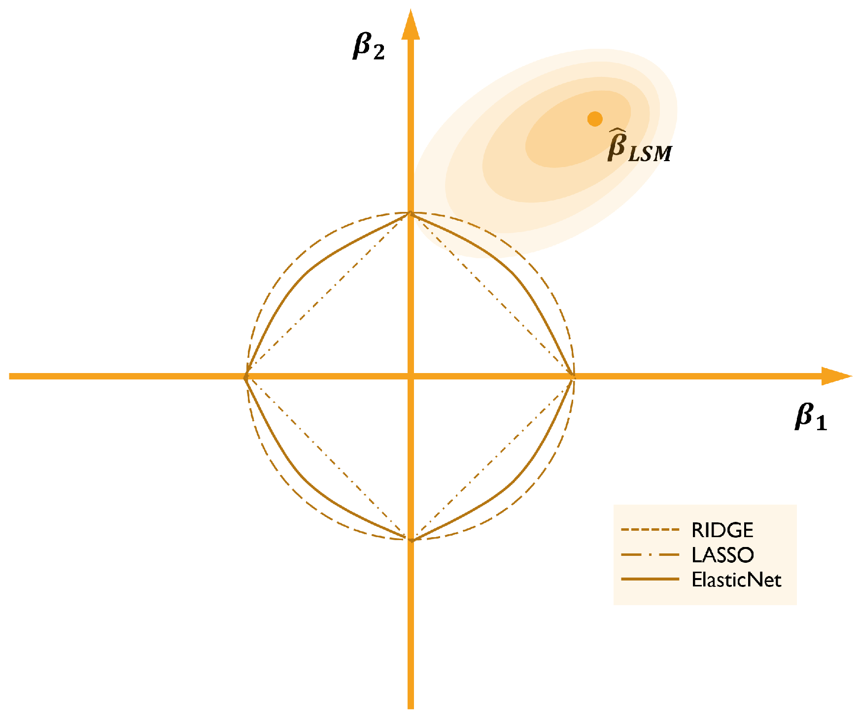
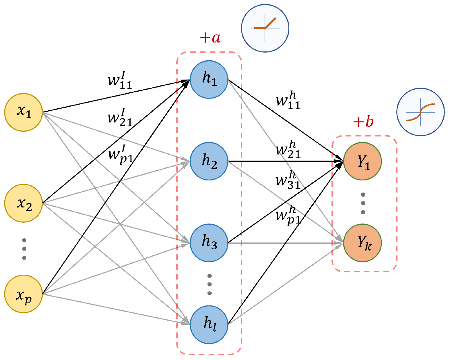
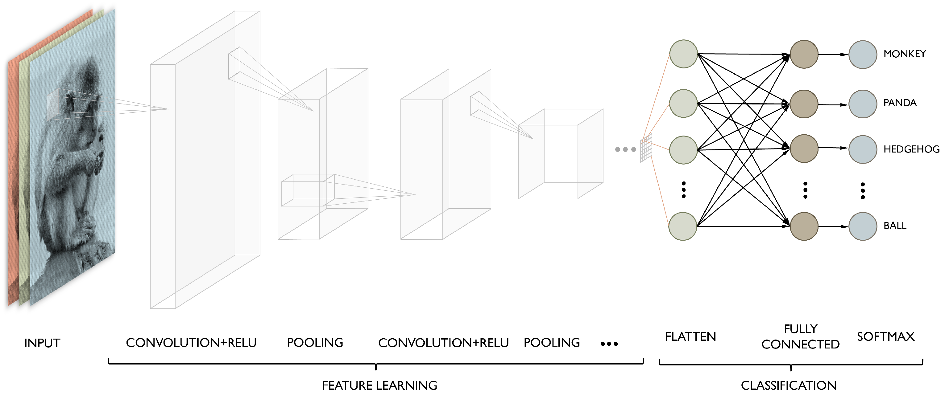
Table 1.
Comparison table between the aforementioned methods on the COCO dataset benchmark.
| Model | Backbone Architecture | Date | Box AP | Mask AP |
|---|---|---|---|---|
| Mask R-CNN | ResNetXt-101-FPN | Jan/2018 | 39.8% | 37.1% |
| SpineNet-190, 1536 × 1536 | Jun/2020 | - | 46.1% | |
| RetinaNet | ResNetXt-101-FPN | Feb/2018 | 40.8% | - |
| SwinV2-G | HTC++ | Nov/2021 | 63.1% | 54.4% |
Publisher’s Note: MDPI stays neutral with regard to jurisdictional claims in published maps and institutional affiliations. |
© 2022 by the authors. Licensee MDPI, Basel, Switzerland. This article is an open access article distributed under the terms and conditions of the Creative Commons Attribution (CC BY) license (https://creativecommons.org/licenses/by/4.0/).
Share and Cite
MDPI and ACS Style
Pinto da Costa, J.F.; Cabral, M. Statistical Methods with Applications in Data Mining: A Review of the Most Recent Works. Mathematics 2022, 10, 993. https://0-doi-org.brum.beds.ac.uk/10.3390/math10060993
AMA Style
Pinto da Costa JF, Cabral M. Statistical Methods with Applications in Data Mining: A Review of the Most Recent Works. Mathematics. 2022; 10(6):993. https://0-doi-org.brum.beds.ac.uk/10.3390/math10060993
Chicago/Turabian StylePinto da Costa, Joaquim Fernando, and Manuel Cabral. 2022. "Statistical Methods with Applications in Data Mining: A Review of the Most Recent Works" Mathematics 10, no. 6: 993. https://0-doi-org.brum.beds.ac.uk/10.3390/math10060993
Note that from the first issue of 2016, this journal uses article numbers instead of page numbers. See further details here.