Article

The Modified Viscosity Approximation Method with Inertial Technique and Forward–Backward Algorithm for Convex Optimization Model

1
Department of Science and Mathematics, Rajamangala University of Technology Isan Surin Campus, Surin 32000, Thailand
2
Faculty of Science, Chiang Mai University, Chiang Mai 50200, Thailand
3
Data Science Research Center, Department of Mathematics, Faculty of Science, Chiang Mai University, Chiang Mai 50200, Thailand
4
Research Group in Mathematics and Applied Mathematics, Department of Mathematics, Faculty of Science, Chiang Mai University, Chiang Mai 50200, Thailand
*
Author to whom correspondence should be addressed.
Submission received: 21 February 2022 / Revised: 15 March 2022 / Accepted: 22 March 2022 / Published: 24 March 2022
(This article belongs to the Special Issue Advanced Optimization Methods and Applications)

Abstract

:
In this paper, we propose a new accelerated algorithm for finding a common fixed point of nonexpansive operators, and then, a strong convergence result of the proposed method is discussed and analyzed in real Hilbert spaces. As an application, we create a new accelerated viscosity forward–backward method (AVFBM) for solving nonsmooth optimization problems of the sum of two objective functions in real Hilbert spaces, and the strong convergence of AVFBM to a minimizer of the sum of two convex functions is established. We also present the application and simulated results of AVFBM for image restoration and data classification problems.

1. Introduction

Image restoration is a fundamental problem in image processing. The image restoration (image deblurring or image deconvolution) is concerned with the reconstruction or estimation of the uncorrupted image from a blurred and noisy image [1,2]. Thus, the main objective of the image restoration algorithms is to reduce the blurring effects and the noise that degraded the image by minimizing the noise of the degraded image to produce an estimate image that approaches the original image.
The image restoration problem can be modeled by a linear inverse problem, which is formulated by:
u = B v + e ,
where B R m × n is the blurring matrix, v R n is an original image, u R m is the observed image, and e R m is a noise. One of the most popular models to solve Problem (1) is the least absolute shrinkage and selection operator (LASSO) [3], which can be considered in the following form:
min v B v u 2 2 + τ v 1 ,
where τ > 0 is a regularization parameter, · 1 is l 1 -norm, and · 2 is l 2 -norm. Moreover, Problem (2) can be applied to solving many areas of science and applied science such as astronomical imaging [4], microscopy [5], and signal recovery problems [6].
The nonsmooth convex optimization model which includes (2) as a particular case has the following form:
min x H ϕ 1 ( x ) + ϕ 2 ( x ) ,
where H is a Hilbert space with norm · , and inner product · , · , ϕ 2 : H R { } is a proper convex and lower semi-continuous function, and ϕ 1 : H R is convex differentiable with a Lipschitz continuous gradient constant L > 0 . The solution set of Problem (3) will be denoted by Ω : = A r g m i n ( ϕ 1 + ϕ 2 ) . Furthermore, x is a solution of Problem (3) if and only if x satisfies the fixed point equation:
x = p r o x c ϕ 2 ( I c ϕ 1 ) ( x ) ,
where c > 0 ,  I is an identity operator, f is the gradient of f ,   p r o x ϕ 2 = ( I + ϕ 2 ) 1 , and ϕ 2 is the subdifferential of ϕ 2 defined by:
ϕ 2 ( a * ) : = { u H : ϕ 2 ( a ) u , a a * + ϕ 2 ( a * ) , a H } ,
see [7,8,9] for more details. For solving (3), the Forward–Backward splitting (FBS) algorithm [10] has been using the following form:
x k + 1 = p r o x c k ϕ 2 backward step ( I c k ϕ 1 ) forward step ( x k ) , k N ,
where x 1 H and 0 < c k < 2 / L . To accelerate the proximal gradient algorithm, the inertial technique or extrapolation technique was proposed by Nesterov in 1983 [11] for solving a class of convex optimization problems (3), where F : = ϕ 1 + ϕ 2 is a smooth and convex function. A typical algorithm takes the following form:
y k = x k + θ k ( x k x k 1 ) , x k + 1 = y k + c F ( y k ) , k N ,
where c > 0 is the step size depending on the Lipschitz continuity modulus of F and the inertial parameter θ k ( 0 , 1 ) for all k . He also showed that by choosing { θ k } such that sup k θ k = 1 , this algorithm has a faster convergence rate than the general gradient algorithm; see [11]. In 2009, Beck and Teboulle [12] improved FBS by using the inertial techniques; this algorithm is known as the fast iterative shrinkage-thresholding algorithm (FISTA), which is defined as follows:
y k = p r o x 1 L ϕ 2 ( x k 1 L ϕ 1 ( x k ) ) , t k + 1 = 1 + 1 + 4 t k 2 2 , θ k = t k 1 t k + 1 , x k + 1 = y k + θ k ( y k y k 1 ) , k N ,
where x 1 = y 0 H ,   t 1 = 1 and θ k is the inertial parameter. The FISTA has been recognized as a fast method. It is noted that the inertial parameter { θ k } in (7) satisfies sup k θ k = 1 . So, the sequence generated by FISTA has a rate of convergence that is proven to be significantly better, both theoretically and practically. Recently, Liang and Schonlieb [13] modified FISTA, called “FISTA-Mod”, for the short and proved weak convergence theorem of FISTA-Mod. Moreover, they proved x k x k 1 = O ( 1 / k ) . The FBS and FISTA are only weak convergence in Hilbert spaces. For strong convergence, the viscosity approximation method (VAM) of the fixed point of a nonexpansive operator T was proposed by Moudafi [14], who proved the strong convergence of the methods (8) in real Hilbert spaces.
x k + 1 = γ k g ( x k ) + ( 1 γ k ) T x k , k N ,
where x 1 H , γ k is a sequence in ( 0 , 1 ) and g is a contraction operator. In 2008, Takahashi [15] modified the viscosity approximation method of Moudafi [14] for finding a common fixed point of a countable family of nonexpansive operators { T k } . His algorithm takes the following form:
x k + 1 = γ k g ( x k ) + ( 1 γ k ) T k x k , k N ,
where x 1 H , { γ k } ( 0 , 1 ) , and g is a contraction operator. He proved a strong convergence theorem of (9) under some conditions on { T k } and { γ k } .
In 2012, He and Guo [16] introduced the following modified viscosity approximation method for a countable family of nonexpansive operators:
x k + 1 = γ k g ( x k ) + ( 1 γ k ) L k x k , k N ,
where { γ k } ( 0 , 1 ) ,   L k = i = 1 k w i s k T i ,   s k = i = 1 k w i , w i > 0 with i = k w k = 1 . They proved strongly the convergence of (10) under the condition on { γ k } without any other condition on { T k } . However, this algorithm needs larger computational work than that of (9). After that, several algorithms for the common fixed points of a countable family of nonexpansive operators were introduced and discussed; see [16,17,18,19,20].
Inspired by [10,12,15], in this paper, we propose a simple method with the inertial technique for solving a common fixed point problem of a countable family of nonexpansive operators in a real Hilbert space. We then prove a strong convergence of the proposed method under some suitable conditions. Finally, we apply our proposed method to solving the image restoration and classification problems.
The rest of this paper is organized as follows: In Section 2, we present some notation and useful lemmas that will be used in this paper. The strong convergence of the accelerated viscosity fixed point method and the accelerated viscosity forward–backward method are analyzed in Section 3. Applications and simulated results for image restoration and data classification problems are given in Section 4. Finally, we give a conclusion remark for further study in Section 5.

2. Preliminaries

In this section, we present some definitions and useful lemmas for proving our main results in the next section. Throughout this paper, we adopt the following notations:
  • H denotes a real Hilbert space with norm · and inner product · , · ;
  • C denotes a nonempty closed convex subset of H ;
  • F i x ( T ) denotes the set of all fixed points of T ;
  • ⇀ and → denote the weak convergence and strong convergence, respectively;
  • p r o x c ϕ 2 ( I c ϕ 1 ) denotes the forward–backward operator of ϕ 1 and ϕ 2 with respect to c .
A mapping T : C C is said to be an L-Lipschitz operator if there exists L > 0 such that T a T b L a b for all a , b C . An L-Lipschitz operator is called a nonexpansive operator and contraction operator if L = 1 and L ( 0 , 1 ) , respectively. If T : C C is a nonexpansive operator with F i x ( T ) , then F i x ( T ) is closed and convex, and the mapping I T is demiclosed at zero, that is for any sequence { x k } C such that x k a and x k T x k 0 imply a F i x ( T ) . A mapping P C is said to be a metric projection of H onto C , if for every a H , there exists a unique nearest point in C denoted by P C a such that:
a P C a a b , b C .
Moreover, P C is firmly nonexpansive mapping and P C satisfying a P C a , b P C a 0 , a H , b C . Let { T k } and Λ be families of nonexpansive operators of C into itself such that F i x ( Λ ) Γ : = k = 1 F i x ( T k ) , where F i x ( Λ ) is the set of all common fixed points of Λ . A sequence { T k } is said to satisfy the NST-condition (I) with Λ [21] if for every bounded sequence { x k } in C ,
lim k x k T k x k = 0 implies lim k x k T x k = 0 for all T Λ .
If Λ is singleton, i.e., Λ = { T } , then { T k } is said to satisfy the NST-condition (I) with T . After that, Aoyama, Kohsaka and Takahashi [22] introduced the condition (Z), which is more general than that of NST-condition (I). A sequence { T k } is said to satisfy the condition (Z) if whenever { x k } is a bounded sequence in C such that lim k x k T k x k = 0 , it follows that every weak cluster point of { x k } belongs to Γ .
It is also known that p r o x c ϕ 2 ( I c ϕ 1 ) is a nonexpansive mapping when 0 < c < 2 / L . The following lemmas are useful for proving our main results.
Lemma 1
([23]). Let  ϕ 1 : H R  be a convex and differentiable function with an L-Lipschitz continuous gradient of  ϕ 1  and let  ϕ 2 : H R { }  be a proper lower semi-continuous and convex function. Let  T k : = p r o x c k ϕ 2 ( I c k ϕ 1 )  and  T : = p r o x c ϕ 2 ( I c ϕ 1 ) , where  c k , c ( 0 , 2 / L )  with  c k c  as  k . Then,  { T k }  satisfies NST-condition (I) with T.
Lemma 2
([24]). For all  a , b H ,  and  t [ 0 , 1 ]  the following hold:
(i)
t a + ( 1 t ) b 2 = t a 2 + ( 1 t ) b 2 t ( 1 t ) a b 2 ;
(ii)
a ± b 2 = a 2 ± 2 a , b + b 2 ;
(iii)
a + b 2 = a 2 + 2 b , a + b .
Lemma 3
([25]). Let { a i , i = 1 , 2 , , k } H . For b i ( 0 , 1 ) , i = 1 , 2 , , k such that i = 1 k b i = 1 . Then, the following identity holds:
i = 1 k b i a i 2 = i = 1 k b i a i 2 i , j = 1 , i j k b i b j a i a j 2 .
Lemma 4
([26]). Let { a k } be a sequence of non-negative real numbers, { b k } be a sequence of real numbers, and { t k } be a sequence of real numbers in ( 0 , 1 ) such that n = 1 t k = . Assume that:
a k + 1 ( 1 t k ) a k + t k b k , k N .
If lim sup i b k i 0 for every subsequence { a k i } of { a k } satisfying the condition:
lim inf i ( a k i + 1 a k i ) 0 ,
then lim k a k = 0 .

3. Main Results

In this section, we propose a new accelerated viscosity fixed point method, which is called “AVFPM” for solving a common fixed point of nonexpansive operators in a real Hilbert space. In order to introduce AVFPM, we assume the following:
  • g : H H is a contraction with constant η ( 0 , 1 ) ;
  • { T k : H H } is a family of nonexpansive operators;
  • { T k } satisfies condition (Z);
  • Γ : = k = 1 F i x ( T k ) .
Theorem 5.
Let { x k } be a sequence generated by Algorithm 1 (AVFPM). Then, { x k } converges strongly to an element a * Γ , where a * = P Γ g ( a * ) .
Now, we prove the strong convergence of Algorithm 1 (AVFPM).
Algorithm 1: An accelerated viscosity fixed point method (AVFPM).
Initialization: Take x 0 , x 1 H arbitrarily and positive sequences { λ k } , { σ k } , { γ k } , { β k } , and { α k } satisfy the following conditions:
{ α k } ( 0 , 1 ) , lim k α k = 0 and k = 1 α k = , { β k } ( 0 , 1 ) , 0 < a 5 γ k < 1 , α k + β k + γ k = 1 , 0 < a 1 λ k a 2 < 1 , 0 < a 3 σ k a 4 < 1 .
for some positive real numbers a 1 , a 2 , a 3 , and a 4 .
Iterative steps: Calculate x k + 1 as follows:
Step 1. Choose a bounded sequence of non-negative real numbers { μ k } . For k 1 , set
θ k = min μ k , τ k x k x k 1 if x k x k 1 , μ k otherwise ,
where { τ k } is a sequence of positive real numbers such that lim k τ k / α k = 0 .
Step 2. Compute
w k = x k + θ k ( x k x k 1 ) , z k = ( 1 λ k ) w k + λ k T k w k , y k = ( 1 σ k ) T k w k + σ k T k z k , x k + 1 = α k g ( w k ) + β k T k z k + γ k T k y k .
Update k : = k + 1 and return to Step 1.
Proof. 
By the Banach contraction principle, there exists a unique a * Γ such that a * = P Γ g ( a * ) . By definitions of x k + 1 , we have:
w k a * x k a * + θ k x k x k 1 ,
and:
z k a * ( 1 λ k ) w k a * + λ k T k w k a * w k a * .
From (12), we get:
y k a * ( 1 σ k ) T k w k a * + σ k T k z k a * w k a * .
From (11)–(13), we obtain:
x k + 1 a * α k g ( w k ) g ( a * ) + α k g ( a * ) a * + β k T k z k a * + γ k T k y k a * α k η w k a * + α k g ( a * ) a * + β k z k a * + γ k y k a * ( 1 α k ( 1 η ) ) w k a * + α k g ( a * ) a * ( 1 α k ( 1 η ) ) x k a * + α k θ k α k x k x k 1 + g ( a * ) a * .
By the condition of θ k , we have lim k θ k α k x k x k 1 = 0 , and so there exists a constant M > 0 such that θ k α k x k x k 1 M k 1 . Thus:
x k + 1 a * ( 1 α k ( 1 η ) ) x k a * + α k ( M + g ( a * ) a * ) .
By mathematical induction, we get:
x k + 1 a * max x 1 a * , M + g ( a * ) a * 1 η k 1 .
This implies that { x k } is bounded and { w k } , { z k } , { y k } , { T k w k } , { T k z k } ,
{ T k y k } , a n d { g ( w k ) } are also bounded. By Lemma 2, we obtain:
w k a * 2 x k a * 2 + θ k 2 x k x k 1 2 + 2 θ k x k a * x k x k 1 ,
and:
z k a * 2 w k a * 2 λ k ( 1 λ k ) w k T k w k 2 .
By Lemma 2(i) and (15), we obtain:
y k a * 2 ( 1 σ k ) T k w k a * 2 + σ k T k z k a * 2 σ k ( 1 σ k ) T k w k T k z k 2 w k a * 2 σ k λ k ( 1 λ k ) w k T k w k 2 σ k ( 1 σ k ) T k w k T k z k 2
From (12), (14), (16), Lemmas 2(iii) and 3, we have:
x k + 1 a * 2 = α k ( g ( w k ) g ( a * ) ) + β k ( T k z k a * ) + γ k ( T k y k a * ) 2 + 2 α k g ( a * ) a * , x k + 1 a * α k g ( w k ) g ( a * ) 2 + β k T k z k a * 2 + γ k T k y k a * 2 + 2 α k g ( a * ) a * , x k + 1 a * α k η w k a * 2 + β k w k a * 2 + γ k w k a * 2 γ k σ k λ k ( 1 λ k ) w k T k w k 2 γ k σ k ( 1 σ k ) T k w k T k z k 2 + 2 α k g ( a * ) a * , x k + 1 a * ( 1 α k ( 1 η ) ) x k a * 2 + α k [ 2 x k a * θ k α k x k x k 1 + θ k α k x k x k 1 θ k x k x k 1 + 2 g ( a * ) a * , x k + 1 a * ] γ k σ k λ k ( 1 λ k ) w k T k w k 2 γ k σ k ( 1 σ k ) T k w k T k z k 2 .
So, we get:
γ k σ k λ k ( 1 λ k ) w k T k w k 2 x k a * 2 x k + 1 a * 2 + α k M ,
and:
γ k σ k ( 1 σ k ) T k w k T k z k 2 x k a * 2 x k + 1 a * 2 + α k M ,
where:
M = sup n 1 2 x k a * θ k α k x k x k 1 + θ k α k x k x k 1 θ k x k x k 1 + 2 g ( a * ) a * , x k + 1 a * .
Now, we show that { x k } converges strongly to a * . Let a k = x k a * 2 . Suppose that { a k i } is a subsequence of { a k } such that lim inf i ( a k i + 1 a k i ) 0 . By (19) and conditions of { λ k } , { σ k } , { γ k } , { β k } , and { α k } , we have:
lim sup i γ k i σ k i ( 1 σ k i ) T k i w k i T k i z k i 2 lim sup i ( a k i a k i + 1 + α k i M ) lim sup i ( a k i a k i + 1 ) + lim sup i α k i M = lim inf i ( a k i + 1 a k i ) 0 .
This implies that:
lim i T k i w k i T k i z k i = 0 .
Similarly, we have lim i w k i T k i w k i = 0 . By definitions of θ k and x k + 1 , we get:
lim i w k i x k i = 0 .
So, we obtain:
x k i T k i x k i x k i T k i w k i + T k i w k i T k i x k i 2 w k i x k i + w k i T k i w k i 0 .
From definitions of x k + 1 , we have:
z k i x k i w k i x k i + λ k i w k i T k i w k i , y k i T k i w k i = σ k i T k i w k i T k i z k i ,
and:
y k i x k i y k i T k i w k i + T k i w k i w k i + w k i x k i .
This implies:
lim i z k i x k i = lim i y k i x k i = 0 .
Moreover,
x k i + 1 x k i x k i + 1 T k i x k i + T k i x k i x k i α k i g ( w k i ) T k i x k i + β k i z k i x k i + γ k i y k i x k i + T k i x k i x k i ,
which implies lim i x k i + 1 x k i = 0 . Now, we claim:
lim sup i g ( a * ) a * , x k i + 1 a * 0 .
Indeed, choose a subsequence { x k i j } of { x k i } such that:
lim sup i g ( a * ) a * , x k i a * = lim j g ( a * ) a * , x k i j a * .
Since { x k i j } is bounded, there exists a subsequence { x k i j p } of { x k i j } such that x k i j p u H . Without loss of generality, we may assume that x k i j u H . Since { T k } satisfies condition (Z), we have u Γ . As lim i x k i + 1 x k i = 0 and a * = P Γ g ( a * ) , we obtain:
lim sup i g ( a * ) a * , x k i + 1 a * = g ( a * ) a * , u a * 0 .
By (17), (28), and lim k θ k α k x k x k 1 = 0 , we can apply Lemma 4 to obtain lim k x k a * = 0 ; that is, { x k } converges strongly to a * = P Γ g ( a * ) . This completes the proof.    □
Finally, we will apply the Algorithm 1 (AVFPM) for solving the nonsmooth convex optimization problems (3) of the sum of two objective functions ϕ 1 and ϕ 2 by assuming the following:
  • g : H H is a contraction with constant η ( 0 , 1 ) ;
  • ϕ 1 : H R is convex differentiable with Lipschitz continuous gradient constant L > 0 ;
  • ϕ 2 : H R { } is a proper convex and lower semi-continuous function;
  • Ω : = A r g m i n ( ϕ 1 + ϕ 2 ) .
By setting T k = p r o x c k ϕ 2 ( I c k ϕ 1 ) , which is the forward–backward operator of ϕ 1 and ϕ 2 with respect to c k ( 0 , 2 / L ) and c k c , we have an accelerated viscosity forward–backward method for solving the problems (3) as follows:
Next, we prove the strong convergence of Algorithm 2 (AVFBM) by using Theorem 5.
Algorithm 2: An accelerated viscosity forward–backward method (AVFBM).
Initialization: Take x 0 , x 1 H arbitrarily and positive sequences { λ k } , { σ k } , { γ k } , { β k } , and { α k } satisfy the following conditions:
{ α k } ( 0 , 1 ) , lim k α k = 0 and k = 1 α k = , { β k } ( 0 , 1 ) , 0 < a 5 γ k < 1 , α k + β k + γ k = 1 , 0 < a 1 λ k a 2 < 1 , 0 < a 3 σ k a 4 < 1 .
for some positive real numbers a 1 , a 2 , a 3 , and a 4 .
Iterative steps: Calculate x k + 1 as follows:
Step 1. Choose a bounded sequence of non-negative real numbers { μ k } . For k 1 , defined θ k by the same as Algorithm 1.
Step 2. Compute
w k = x k + θ k ( x k x k 1 ) , z k = ( 1 λ k ) w k + λ k p r o x c k ϕ 2 ( I c k ϕ 1 ) w k , y k = ( 1 σ k ) p r o x c k ϕ 2 ( I c k ϕ 1 ) w k + σ k p r o x c k ϕ 2 ( I c k ϕ 1 ) z k , x k + 1 = α k g ( w k ) + β k p r o x c k ϕ 2 ( I c k ϕ 1 ) z k + γ k p r o x c k ϕ 2 ( I c k ϕ 1 ) y k .
Update k : = k + 1 and return to Step 1.
Theorem 6.
Let { x k } be a sequence generated by Algorithm 2 (AVFBM). Then, { x k } converges strongly to an element a * Ω , where a * = P Ω g ( a * ) .
Proof. 
Let T : = p r o x c ϕ 2 ( I c ϕ 1 ) and T k : = p r o x c k ϕ 2 ( I c k ϕ 1 ) . Then, T and { T k } are nonexpansive operators for all k , and F i x ( T ) = k = 1 F i x ( T k ) = A r g m i n ( ϕ 1 + ϕ 2 ) . By Lemma 1, we have { T k } , which satisfies condition (Z). Therefore, we obtain the result directly by Theorem 5. □

4. Application and Simulated Results

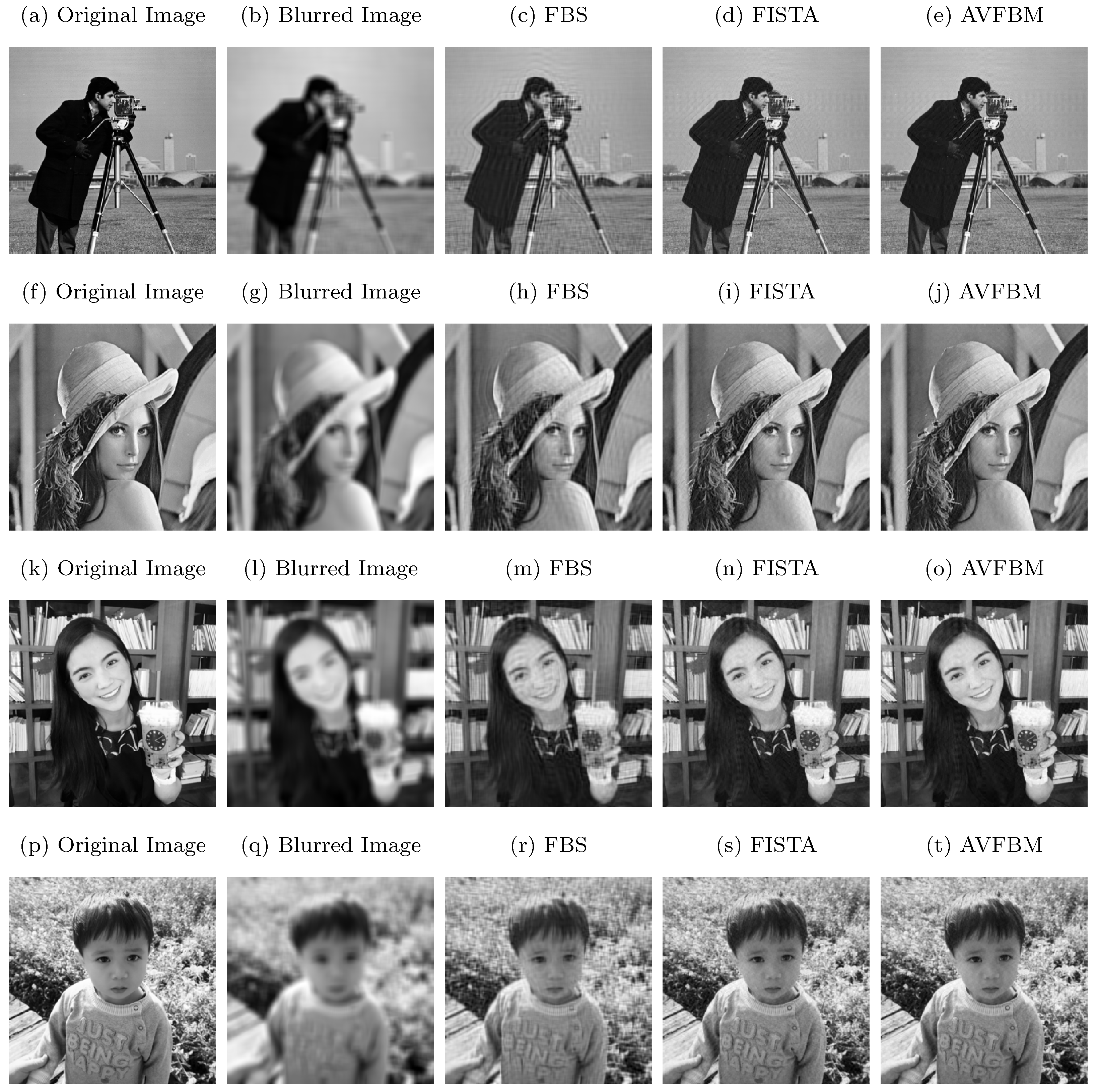
4.1. Image Restoration

In this example, we apply Algorithm 2 (AVFBM) to solving an image restoration problem (2) and compare the deblurring efficiency of AVFBM, FBS [10], and FISTA [12]. Our programs are written in MATLAB and run on a laptop with an Intel core i5, 4.00 GB RAM, and windows 8 (64-bit). All algorithms applied to the l 1 -regularization problem (2); that is, ϕ 1 ( x ) = B x b 2 2 and ϕ 2 ( x ) = τ x 1 , where B is the blurring operator, b is the observed image, and τ is the regularization parameter. The maximum iteration number for all methods was fixed at 500.
In these experiments, we consider four gray-scale images (Cameraman, Lenna, Woman, and Boy) with size of 256 × 256 as the original images and consider Gaussian blur of filter size 9 × 9 with a standard deviation σ = 4 with noise 10 4 . We have measured the performance of AVFBM, FBS, and FISTA by means of the Signal-to-Noise Ratio (SNR) [27] and Peak Signal-to-Noise Ratio (PSNR) [28]. The SNR and PSNR at x k of the restored images are defined as:
S N R ( x , x k ) = 10 log 10 x x ¯ 2 x k x 2 ,
P S N R ( x k ) = 10 log 10 255 2 M S E ,
where M S E = 1 256 2 x k x 2 2 , x is the original image, and x ¯ is the mean of the original image. The regularization parameter was chosen to be τ = 10 4 , and the initial image was the blurred image. The Lipschitz constant L of the gradient f is L = 2 λ m a x ( B T B ) [12]. The parameters of the algorithms are chosen as follows: λ k = 0.5 k k + 1 , σ k = 0.99 k k + 1 , α k = 1 50 k , β k = 1 300 k + 1 , γ k = 1 α k β k , c k = k L ( k + 1 ) , c = 1 L , τ k = 10 15 k 2 and μ k = t k 1 t k + 1 , where t k is a sequence defined by t 1 = 1 and t k + 1 = 1 + 1 + 4 t k 2 2 . The contraction mapping is defined by g ( a ) = 0.95 a for all a R n . The comparison of the performance of AVFBM, FISTA, and FBS by means of SNR and PSNR is shown in Figure 1. The plot of SNR and PSNR at x k of the restored images is shown in Figure 2. We see from Figure 1 and Figure 2 that AVFBM gives a higher performance of SNR and PSNR than the other methods. The comparison results for deblurring of the three methods of the four images are shown in Figure 3.

4.2. Data Classification

In this section, a learning algorithm named extreme learning machine (ELM) [29] will be investigated. ELM is a learning algorithm for single-hidden layer feedforward neural networks (SLFNs). Let D = { ( x i , t i ) : x i R n , t i R m , i = 1 , 2 , , N } be a training dataset with N distinct training data x i and label t i . For a given M nodes in the hidden layer, the SLFNs output for the jth pattern, o j R m , is given by:
o j = i = 1 M w i f ( h i , x j + b i ) , j = 1 , 2 , , N ,
where f is the activation function, h i R n and b i R for i = 1 , 2 , , M are the weight vector and bias connecting the input layer to the ith hidden node, respectively, and w i R m for i = 1 , 2 , , M is the weight vector connecting the ith hidden layer to the output layer. The target of SLFNs is to approximate the parameters w i , h i , b i for all i = 1 , 2 , , M such that:
t j = i = 1 M w i f ( h i , x j + b i ) , j = 1 , 2 , , N ,
which means that zero error i = 1 N o i t i is close to 0 while ELM is used to find only parameter w i with random h i and b i . As the above N equations, Equation (30) can be rewritten as:
Hw = T
where:
H = f ( h 1 , x 1 + b 1 ) f ( h M , x 1 + b M ) f ( h 1 , x N + b 1 ) f ( h M , x N + b M ) N × M ,
w = w 1 T , , w M T m × M T and T = t 1 T , , t N T m × N T . From Equation (31), the ELM learning algorithm estimates the weight w by w = H T where H = ( H T H ) 1 H T is the pseudo-inverse matrix of H . Note that the linear system (31) can be represented by a least squared method. As shown in [29], ELM has an extremely fast training speed and good generalization performance. Nevertheless, its solutions also have some drawbacks [30]. To overcome these drawbacks, regularized extreme learning machine (RegELM) [30] replacing the least square method by the regularization method, i.e., ridge regression, for the training model was proposed, and the mathematical model of the RegELM algorithm can be described as:
min w R M × m 1 2 Hw T 2 2 + λ 2 w 2 2 ,
where λ > 0 is called the regularization parameter. The RegELM’s output weight can be calculated by w = ( λ I + H T H ) H T T , where I is the identity matrix. Although RegELM can be expected to provide better generalization ability than ELM and its running time is extremely fast similarly to ELM, we can define a greater generalization of RegELM as in [31] by replacing Equation (32) in a generalized way as follows:
min w R M × m 1 2 Hw T 2 2 + λ [ ( 1 α ) 1 2 w 2 2 + α w 1 ] ,
where 0 α 1 . Equation (33), called elastic net, trades off between the ride regression ( α = 0 ) and the LASSO ( α = 1 ). In this paper, we present a new algorithm for RegELM and employ our results to data classification problems with benchmark datasets. For this case, we set α = 1 , and Problem (33) becomes a LASSO problem. From our result (Theorem 6) in Section 3, we can apply AVFBM (Algorithm 2) to solve the LASSO problem and define a learning algorithm for RegELM as follows:
RegELM-AVFBM: Given a training set D = { ( x i , t i ) : x i R n , t i R m , i = 1 , 2 , , N } , activation function f,
  • Step 1: Select regularization parameter λ and hidden node number M.
  • Step 2: Randomly h i and b i , i = 1 , , M .
  • Step 3: Calculate the hidden layer output matrix H .
  • Step 4: Obtain the output weight w by using AVFBM (Algorithm 2).
Several benchmark problems were chosen for experiments. All datasets were downloaded from https://archive.ics.uci.edu/ (accessed on 6 April 2020). The information of each dataset viz name of datasets, the number of attributes (number of input nodes), the number of classes (number of output nodes), and the number of (sample) data are summarized in Table 1. Each dataset was normalized to zero mean and unit variance; 70% of the data were sampled for training, and the remaining 30% were used for testing. For each method, we tested a different number of hidden nodes M in order to see which architecture provided the best results. The number of nodes in the hidden layer varied from 1 to 200 for the abalone dataset and from 1 to 100 for the other five datasets. For each method, we set the sigmoid function as the activation function f and the regularization parameter λ = 1 × 10 5 for regularized methods (RegELM and RegELM-AVFBM). However, for approximation methods (AVFBM, FISTA), we use relative error criteria, x k x k 1 x k < ϵ , for the stopping algorithm and set all control sequences ( λ k , σ k , α k , β k , γ k , c k , τ k , μ k ) as in Section 4.1. For evaluating the performance of each method, an accuracy is defined as the total accuracy rate of classifying each case correctly. Accuracy is a value that represents the power of a model to correctly predict, and it is described as follows.
A c c u r a c y = ( T P + T N ) / ( T P + F P + T N + F N ) .
In experimental results, the accuracy of training and testing in percentage and the suitable number of hidden nodes of our method compared with direct methods viz standard ELM [29] and RegELM [30] are described in Table 2. RegELM-AVFBM has a good behavior in terms of accuracy of prediction and fit for testing datasets compared with the two direct methods. However, it is hard to compare the computational time, since approximation methods take time to iterate for convergence to the solution. Thus, to evaluate in the same way, we use two approximation methods (FISTA and AVFBM) for training RegELM and train the model with five different stopping errors ϵ under a maximum of 100,000 iterations. Table 3 shows the performance viz accuracy of training and testing (in percentage), computational time (in second), number of computed iterations, and number of suitable nodes in the hidden layer.

5. Conclusions

In this work, by using the inertial technique together with the viscosity approximation method, we propose a new accelerated algorithm for finding a common fixed point of a countable family of nonexpansive operates in a real Hilbert space. The strong convergence of the proposed method is established under some suitable conditions. As a special case, we obtain a new accelerated algorithm, called the accelerated viscosity forward–backward method (AVFBM), for solving nonsmooth convex optimization problems. We also apply our algorithm, AVFBM, to solving image restoration and classification problems. By our experiments, for image restoration problem, they show that our algorithm, AVFBM, has a better performance for SNR and PSNR than that of FBS and FISTA, which are the most popular methods for solving such problems. Moreover, for the classification problems of six datasets—Zoo, Iris, Wine, Parkinsons, Heart Disease UCI, and Abalone (https://archive.ics.uci.edu/, accessed on 6 April 2020)—we use our algorithm, AVFBM, as a learning algorithm for finding the optimal output weight w in the mathematical model (32) of the classification problems. We compare the efficiency of our method with ELM, RegELM, and RegELM-FISTA by using the measurement of accuracy of training and testing. We found that our algorithm outperforms the other methods, as seen from Table 2 and Table 3.

Author Contributions

Formal analysis, writing—original draft preparation, A.H.; methodology, writing—review and editing, software, L.B.; Conceptualization, revised the manuscript, S.S. All authors have read and agreed to the published version of the manuscript.

Funding

This work was supported by Chiang Mai University and NSRF [grant number B05F640183].

Institutional Review Board Statement

Not applicable.

Informed Consent Statement

Not applicable.

Data Availability Statement

Not applicable.

Acknowledgments

This research has received funding support from the NSRF via the program Management Unit for Human Resources & Institutional Development, Research and Innovation [grant number B05F640183] and Chiang Mai University. The first author would like to thank Rajamangala University of Technology Isan for partial financial support and L. Bussaban was supported by the Thailand Research Fund through the Royal Golden Jubilee (RGJ) PhD Programme (Grant No. PHD/0184/2560).

Conflicts of Interest

The authors declare that they have no competing interest.

References

  1. Maurya, A.; Tiwari, R. A Novel Method of Image Restoration by using Different Types of Filtering Techniques. Int. J. Eng. Sci. Innov. Technol. 2014, 3, 124–129. [Google Scholar]
  2. Suseela, G.; Basha, S.A.; Babu, K.P. Image Restoration Using Lucy Richardson Algorithm For X-Ray Images. IJISET Int. J. Innov. Sci. Eng. Technol. 2016, 3, 280–285. [Google Scholar]
  3. Tibshirani, R. Regression shrinkage and selection via the lasso. J. R. Stat. Soc. B Methodol. 1996, 58, 267–288. [Google Scholar]
  4. Vogel, C. Computational Methods for Inverse Problems; SIAM: Philadelphia, PA, USA, 2002. [Google Scholar]
  5. Sluder, G.; Wolf, D.E. Digital Microscopy, 3rd ed.; Elsevier: New York, NY, USA, 2007. [Google Scholar]
  6. Suantai, S.; Kankam, K.; Cholamjiak, P. A Novel Forward-Backward Algorithm for Solving Convex Minimization Problem in Hilbert Spaces. Mathematics 2020, 8, 42. [Google Scholar] [CrossRef] [Green Version]
  7. Bauschke, H.H.; Combettes, P.L. Convex Analysis and Monotone Operator Theory in Hilbert Spaces; Springer: New York, NY, USA, 2011. [Google Scholar]
  8. Burachik, R.S.; Iusem, A.N. Set-Valued Mappings and Enlargements of Monotone Operators; Springer Science Business Media: New York, NY, USA, 2007. [Google Scholar]
  9. Moreau, J.J. Proximité et dualité dans un espace hilbertien. B. Soc. Math. Fr. 1965, 93, 273–299. [Google Scholar]
  10. Lions, P.L.; Mercier, B. Splitting algorithms for the sum of two nonlinear operators. SIAM J. Numer. Anal. 1979, 16, 964–979. [Google Scholar]
  11. Nesterov, Y.E. A method for solving the convex programming problem with convergence rate O(1/k2). Sov. Math. Dokl. 1983, 27, 372–376. [Google Scholar]
  12. Beck, A.; Teboulle, M. A fast iterative shrinkage-thresholding algorithm for linear inverse problems. SIAM J. Imaging Sci. 2009, 2, 183–202. [Google Scholar]
  13. Liang, J.; Schonlieb, C.B. Improving fista: Faster, smarter and greedier. arXiv 2018, arXiv:1811.01430. [Google Scholar]
  14. Moudafi, A. Viscosity approximation method for fixed-points problems. J. Math. Anal. Appl. 2000, 241, 46–55. [Google Scholar]
  15. Takahashi, W. Viscosity approximation methods for countable families of nonexpansive mappings in Banach spaces. Nonlinear Anal. 2009, 70, 719–734. [Google Scholar]
  16. He, S.; Guo, J. Iterative algorithm for common fixed points of infinite family of nonexpansive mappings in Banach spaces. J. Appl. Math. 2012, 2012, 787419. [Google Scholar]
  17. Shimoji, K.; Takahashi, W. Strong convergence to common fixed points of infinite nonexpansive mappings and applications. Taiwan. J. Math. 2001, 5, 387–404. [Google Scholar]
  18. Aoyama, K.; Kimura, Y.; Takahashi, W.; Toyoda, M. Finding common fixed points of a countable family of nonexpansive mappings in a Banach space. Sci. Math. Jpn. 2007, 66, 325–335. [Google Scholar]
  19. Takahashi, W.; Takeuchi, Y.; Kubota, R. Strong convergence theorems by hybrid methods for families of nonexpansive mappings in Hilbert spaces. J. Math. Anal. Appl. 2008, 341, 276–286. [Google Scholar]
  20. Takahashi, W.; Yao, J.-C. Strong convergence theorems by hybrid methods for countable families of nonlinear operators in Banach spaces. J. Fixed Point Theory Appl. 2012, 11, 333–353. [Google Scholar]
  21. Nakajo, K.; Shimoji, K.; Takahashi, W. Strong convergence to common fixed points of families of nonexpansive mappings in Banach spaces. J. Nonlinear Convex Anal. 2007, 8, 11–34. [Google Scholar]
  22. Aoyama, K.; Kohsaka, F.; Takahashi, W. Strong convergence theorems by shrinking and hybrid projection methods for relatively nonexpansive mappings in Banach spaces. In Proceedings of the 5th International Conference on Nonlinear Analysis and Convex Analysis, Hakodate, Japan, 26–31 August 2009; pp. 7–26. [Google Scholar]
  23. Bussaban, L.; Suantai, S.; Kaewkhao, A. A parallel inertial S-iteration forward-backward algorithm for regression and classification problems. Carpathian J. Math. 2020, 36, 35–44. [Google Scholar]
  24. Takahashi, W. Introduction to Nonlinear and Convex Analysis; Yokohama Publishers: Yokohama, Japan, 2009. [Google Scholar]
  25. Chidume, C.E.; Ezeora, J.N. Krasnoselskii-type algorithm for family of multi-valued strictly pseudo-contractive mappings. Fixed Point Theory Appl. 2014, 2014, 111. [Google Scholar] [CrossRef] [Green Version]
  26. Saejung, S.; Yotkaew, P. Approximation of zeros of inverse strongly monotone operators in Banach spaces. Nonlinear Anal. 2012, 75, 724–750. [Google Scholar]
  27. Chen, D.Q.; Zhang, H.; Cheng, L.Z. A fast fixed point algorithm for total variation deblurring and segmentation. J. Math. Imaging Vis. 2012, 43, 167–179. [Google Scholar]
  28. Thung, K.; Raveendran, P. A survey of image quality measures. In Proceedings of the 2009 International Conference for Technical Postgraduates (TECHPOS), Kuala Lumpur, Malaysia, 14–15 December 2009; pp. 1–4. [Google Scholar]
  29. Huang, G.B.; Zhu, Q.Y.; Siew, C.K. Extreme learning machine. Neurocomputing 2006, 70, 489–501. [Google Scholar]
  30. Deng, W.; Zheng, Q.; Chen, L. Regularized extreme learning machine. In Proceedings of the 2009 IEEE Symposium on Computational Intelligence and Data Mining, Nashville, TN, USA, 30 March–2 April 2009; pp. 389–395. [Google Scholar]
  31. Martínez-Martínez, J.M.; Escandell-Montero, P.; Soria-Olivas, E.; Martín-Guerrero, J.D.; Magdalena-Benedito, R.; Gómez-Sanchis, J. Regularized extreme learning machine for regression problems. Neurocomputing 2011, 74, 3716–3721. [Google Scholar]
Figure 1. Comparison of SNR and PSNR by FBS, FISTA, AVFBM.
Mathematics 10 01036 g001
Figure 2. Plot of SNR and PSNR for the images.
Mathematics 10 01036 g002
Figure 3. Original images, blurred images, and Deblurring images by FBS, FISTA, AVFBM.
Mathematics 10 01036 g003
Table 1. Information of benchmark datasets.
Datasets# Attributes# Classes# Observations
# Train (≈70%)# Test (≈30%)
Zoo1677031
Iris4310545
Wine13312850
Parkinsons23213560
Heart Disease UCI14221390
Abalone8329241253
Note that the cardinal number of set A is denoted by #A. For example, # Attributes is the number of attributes of the data.
Table 2. Comparison of the accuracy of training and testing as well as the number of hidden nodes for ELM, RegELM, and RegELM-AVFBM.
DatasetsELMRegELMRegELM-AVFBM
Training (%)Testing (%)# NodesTraining (%)Testing (%)# NodesTraining (%)Testing (%)# Nodes
Zoo97.142993.54841397.142993.54841310096.774293
Iris99.04761006098.09521004298.095210054
Wine98.43751003698.43751003610010040
Parkinsons94.8148753194.8148753196.296381.666778
Heart Disease UCI86.38584.44442586.38584.44442588.732485.555633
Abalone69.049267.43818969.049267.43818968.433767.518111
Table 3. Comparison of the accuracy of training and testing, computation time, number of iterations, and number of hidden nodes for RegELM-FISTA and RegELM-AVFBM. The sign in the column # Iters means that the model was computed over the maximum iterations (100,000 iterations for this case).
Datasets ϵ RegELM-FISTARegELM-AVFBM
Training (%)Testing (%)Time(s)# Iters# NodesTraining (%)Testing (%)Time(s)# Iters# Nodes
Zoo0.19090.32260.0005994113398.571493.54840.0008407982
0.0198.571493.54840.0021261407210096.77420.00792088193
0.00110093.548390.00854054554298.5714393.548390.00520315713
0.000197.14285793.5483870.015265613301397.1428693.548390.014222538413
0.0000197.14285793.5483870.035352826091397.1428693.548390.019383669413
0.00000197.14285793.5483870.056133741931397.14285793.5483870.0317928135413
Iris0.179.047691.11110.000650611398091.11110.0003463720
0.018091.11110.000854427996.190481000.003307511056
0.00192.3809597.777780.01413146582298.095241000.021739180454
0.000196.1904761000.05171542323898.0952381000.1359273489153
0.0000198.09523811000.624277841,5845698.09523811000.998174547,69542
0.000001--------
Wine0.197.6563960.0005292113199.2188980.0008743865
0.0199.2188980.001597930641001000.00471119840
0.00199.218751000.01067583644598.43751000.00629827136
0.000198.43751000.053602543743698.43751000.0234622114636
0.0000198.43751000.215090418,4063698.43751000.0710794313536
0.00000198.43751000.473309439,1083698.43751000.1426151734236
Parkinsons0.180.7407750.000536211580.740773.33330.000784345
0.0180.7407750.00031611596.296381.666670.003492711178
0.00196.296378.333330.01433036498395.5555676.666670.009272225231
0.000198.518519850.107251247029510076.6666670.0401135153360
0.0000199.259259378.33333330.369355131,4886095.555556750.0395779226631
0.00000195.5555556750.306722732,1853194.814815750.0887627542131
Heart Disease UCI0.182.629184.44440.000561115286.854585.55560.0006593872
0.0184.976584.44440.0008177315785.915584.44440.00276267325
0.00187.7934386.666670.01157456006188.7323985.555560.005146624033
0.000190.14084585.5555560.130025452315886.3849884.444440.013131764425
0.0000186.38497784.4444440.062938565072586.38497784.4444440.042063170725
0.00000186.384976584.44444440.124522212,5052586.38497784.4444440.054982336625
Abalone0.157.284556.34480.000833211957.010956.6640.0007203716
0.0159.1313357.861130.01164774714766.7236766.00160.019906711196
0.00164.7400864.086190.0777244511168.6388567.118910.2978755817175
0.000166.79206666.4006380.820114755609668.43365367.5179570.95156344480111
0.0000168.536251767.198723111.926980351,90014968.741450167.67757383.482610421,87789
0.000001----68.946648467.677573813.056653181,39289
Publisher’s Note: MDPI stays neutral with regard to jurisdictional claims in published maps and institutional affiliations.

