An Analysis of Travel Patterns in Barcelona Metro Using Tucker3 Decomposition

Abstract

In recent years, a growing number of large, densely populated cities have emerged, which need urban traffic planning and therefore knowledge of mobility patterns. Knowledge of space-time distribution of passengers in cities is necessary for effective urban traffic planning and restructuring, especially in large cities. In this paper, the inbound ridership in the Barcelona metro is modelled into a three-way tensor so that each element contains the number of passenger in the ith station at the jth time on the kth day. Tucker3 decomposition is used to discover spatial clusters, temporal patterns, and the relationships between them. The results indicate that travel patterns differ between weekdays and weekends; in addition, rush and off-peak hours of each day have been identified, and a classification of stations has been obtained.

1. Introduction

Currently, approximately 50% of the world’s population lives in cities and, according to a report by the United Nations, this proportion is estimated to increase to 68% by 2050 [1]. Hence, one of the main sustainable development goals (SDG) promoted by the United Nations is the improvement of public transport systems. This implies improvement not only in the construction of better and more modern and sustainable infrastructures, but also in the design and implementation of protocols and methodologies to manage the transport networks in a more efficient way. The latter relies primarily on the use of mathematical and statistical techniques for designing such management tools.

Automated fare collection (AFC) systems are used in most public transport networks (bus, light railway, and metro, etc.). Because people must present the smart cards when entering a station, travel data such as the origin station and the boarding time are recorded in these systems. Therefore, these systems collect a large amount of information that can be used for the study of urban mobility patterns.

One of the most used means of transportation in large cities are metro systems, due to their high speed and capacity [2]. Knowledge of the spatial and temporal distribution of passengers in these systems is very important for efficient planning and precise operation. In recent years, many studies of the metro systems, from both mathematical and statistical perspectives, have emerged in the literature. Most of them focus on passenger forecasting [3,4,5,6] and human mobility patterns [2,7,8,9,10,11]. For instance, ref [9] proposed a k-medoids clustering analysis approach to analyze subway stations in Nanjing (China) and compared the results obtained with previous studies; ref [10] developed a new method to mine metro commuting mobility patterns using massive smart card data in Chongqing (China); ref [11] examined changes in travel behavior based on yearly activity profiles using 3 years of longitudinal smart card data; ref [3] proposed a hybrid EMD–BPN forecasting approach that combines empirical mode decomposition (EMD) and back-propagation neural networks (BPN) to predict the short-term passenger flow in metro systems; and finally, ref [6] proposed a new approach called the seasonal and nonlinear least squares support vector machine (SN-LSSVM) to extract the periodicity and non linearity characteristics of passenger flow.

Urban mobility patterns can be analyzed through the data obtained from smart cards. However, the datasets are huge and complex to analyze. In most cases, a two-dimensional matrix and techniques such as principal component analysis (PCA) [12] and clustering methods [13,14] are used [15]. Nonetheless, with these approaches, there is a significant loss of information, as the original structure of the data is broken [2]. Using tensors, the original structure of the data can be preserved so the information of different dimensions can be analyze at the same time. CANDECOMP/PARAFAC (CP) [16,17] and the Tucker3 [18] decomposition are the most used methods for tensor decomposition.

In the literature, tensor decomposition has previously been used to analyze transport networks: [19] used a regularized non-negative Tucker decomposition (rNTD) method to discover the urban spatio-temporal structure from time-evolving traffic networks; ref [20] proposed a grey prediction model for short-time traffic flows based on tensor decomposition; a tensor-based framework combining with “priori modeling” and “posterior analysis” to forecast peak-hour passenger was proposed by [5]; a hybrid approach combining the tensor decomposition and clustering techniques was presented in [21] to extract the features of traffic flow of urban road networks; a mobility pattern mining framework based on a non-negative tensor model called BetaNTF was proposed and applied to analyze bike sharing network mobility data in Boston, MA [22]; a sparsity constraint nonnegative tensor factorization (SNTF) method was used to study mobility patterns from the location based social networks (LBSNs) usage data [23]; a multi-way probabilistic factorization model based on the concept of tensor decomposition and probabilistic latent semantic analysis (PLSA) was applied on a four-way dataset recording 14 million public transport journeys extracted from smart card transactions in Singapore [24]; in ref [25], a non-negative tensor factorization was used to extract underlying spatio-temporal movement patterns from large-scale urban trajectory data; and finally, ref [2] applied NCP tensor decomposition to discover the main characteristics of travel patterns in the metro network of Shenzhen in China.

The use of tensors goes back to the 20th century when tensors emerged in psychometrics and chemometrics for multi-way data analysis [26,27]. Tensor decomposition began to be used in the study of signal processing in the 1990s [28,29]. Currently, it has become a very useful mathematical tool in artificial intelligence. This has contributed significantly to the popularization of tensors as tools for data analysis, where tensors are commonly used in data mining and machine learning. Machine learning applications include face recognition, temporal analysis (discovering patterns, predicting evolution, and spotting anomalies) and medical diagnosis, amongst others.

The main goal of this study was to identify mobility patterns in Barcelona metro users through the Tucker3 decomposition. That is, to determine the spatial, temporal and spatio-temporal patterns. In this paper, data from smart cards are modeled using a three way tensor, so that each element contains the number of passengers in the ith station at the jth time on the kth day. By using tensors, the original structure of the smart card data from metro systems is maintained and, therefore, the information of different dimensions can be analyzed at the same time. Multidimensional features can be extracted from the data through the Tucker3 decomposition, reducing the dimensions of each mode (stations, timetable, and days) and exploring how the different modes interact with each other. The data matrix is decomposed into three matrices (component matrices) and a core matrix, which models the dynamic relationships among them. The temporal patterns are obtained from these matrices and the stations are grouped according to the patterns found.

Mobility patterns in the Barcelona metro have been previously analyzed by [30], who applied principal component analysis (PCA) and clustering techniques and obtained a classification of the stations according to their patterns of use. The main advantage of the approach proposed here is that patterns are also established in the days of the week and the timetables.

The remainder of the paper is organized as follows: the methodology used in this work is presented in Section 2. In Section 3, the daily mobility patterns are analyzed based on the tensor decomposition results. Finally, Section 4 summarizes the conclusions obtained.

2. Methodology

Tensors can be defined as multidimensional arrays [31]. The order of a tensor, also known as way or mode, is the number of dimensions it has. Therefore, first order tensors are vectors, $\mathbf{x}\in {\mathbb{R}}^{I_1}$; second order tensors are matrices, $\mathbf{X}\in {\mathbb{R}}^{I_1\times I_2}$; and tensors of order three or higher are known as higher-order tensors $\underline{\mathbf{X}}\in {\mathbb{R}}^{I_1\times I_2\times \dots \times I_N}$. This work focuses on three-way arrays, as the data collected from smart cards can be organized following this structure.

Tensor decompositions are higher order generalizations of the matrix singular value decomposition (SVD) and principal component analysis (PCA). The most important tensor decompositions are the canonical polyadic decomposition (CPD) [16,17] and the Tucker3 [18] decomposition.

The Tucker3 [18] decomposition decomposes a three-way array X of order $I\times J\times K$ into $I\times P$, $J\times Q$, and $K\times R$ component matrices $\mathbf{A}$, $\mathbf{B}$, and $\mathbf{C}$ and a $P\times Q\times R$ weight array $\underline{\mathbf{G}}$, being the complexity of the model $(P,Q,R)$ (see Figure 1).

In scalar notation, the Tucker3 model (T3) can be written as follows:

$$x_{ijk}=\sum _{p=1}^P\sum _{q=1}^Q\sum _{r=1}^R{a}_{ip}{b}_{jq}{c}_{kr}{g}_{pqr}+e_{ijk},$$

(1)

where $a_{ip}$, $b_{jp}$, and $c_{kr}$ denote the component scores of the ith element on the pth component for the A-mode, of the jth element on the qth component for the B-mode, and of the kth element on the rth component for the C-mode, respectively. The entries $g_{pqr}$ denote the elements of the core array $\underline{\mathbf{G}}$ and reflect the interaction among the components of the three modes, and $e_{ijk}$ is an error term.

In addition, the Tucker3 model can be written in matrix notation as follows:

$${\mathbf{X}}_A=\mathbf{A}{\mathbf{G}}_A({\mathbf{C}}^T\otimes {\mathbf{B}}^T)+{\mathbf{E}}_A,$$

(2)

where ⊗ denotes the Kronecker product, and ${\mathbf{X}}_A$, ${\mathbf{G}}_A$, and ${\mathbf{E}}_A$ denote the $I\times JK$, $P\times QR$, and $I\times JK$ matricizations of $\underline{\mathbf{X}}$, $\underline{\mathbf{G}}$, and $\underline{\mathbf{E}}$, respectively [32].

The Tucker3 algorithm is based on minimization of the sum of the squared errors:

$$\parallel {\mathbf{E}}_A{\parallel }^2={\parallel {\mathbf{X}}_A-\mathbf{A}{\mathbf{G}}_A{(\mathbf{C}\otimes \mathbf{B})}^T\parallel }^2.$$

(3)

To achieve this goal an alternating least square (ALS) algorithm is used [33].

It should be noted that the parameters of the Tucker3 model can only be uniquely identified upon a joint permutation, scaling, reflection, and rotation of the components and/or the core array [27]. To partially identify the solution, it was decided to constrain A, B, and C to be columnwise orthonormal.

Tucker3 model indeterminacy can be used to transform the component matrices and the core matrix to simple structures to facilitate its interpretation. That is, it is about finding a solution where most of the component scores are close to zero and only a few have high values, in an absolute sense.

In general, no a priory information is available regarding the optimal rank (P,Q,R) underlying a Tucker3 model for a dataset at hand. As an alternative, researchers may perform different analyses with varying complexities in which the rank of the model goes from (1,1,1) to ($P_{max}$,$Q_{max}$,$R_{max}$) and select a model that has a good balance between model fit ($f_i$) and model complexity ($c_i$). Model (mis)fit may be quantified by the the sum of squared residuals or the amount of explained variance, whereas different options exist to define model complexity, like the total number of components (i.e., $P+Q+R$), the total number of fitted parameters (i.e., $IP+JQ+KR+PQR+LP$), and the number of free parameters (i.e., $IP+JQ+KR+PQR+LP-P^2-Q^2-R^2$) [34,35].

It is important to highlight that models for which $Q>PR$ or $R>PQ$ should not be considered, as it can be shown that there exists models that are more parsimonious (i.e., have a smaller number of fitted parameters) that fit the data equally well [36].

The optimal rank of a Tucker3 model may be identified by using the CHull procedure [34,36], which is an automated heuristic for model selection. Starting from a fit $f_i$ and complexity $c_i$ value for all valid T3-PCA solutions with a rank between (1,1,1) and (Pmax,Qmax,Rmax), the CHull method goes through the following two steps: (1) determining the models $m_i$ ($i=1,\dots ,M$) that are located on the (lower) boundary of the convex hull of the $c_i$ by $f_i$ complexity-by-fit plot of all the valid models and (2) identifying the model on the boundary of the convex hull that optimally balances model fit and model complexity. To this end, one may use an automated procedure by computing for each model $m_i$ the corresponding $st$-ratio:

$$s{t}_i=\frac{(f_{i-1}-f_i)/(c_i-c_{i-1})}{(f_i-f_{i+1})/(c_{i+1}-c_i)},$$

(4)

and selecting the model with the largest $st$-value.

3. Data Analysis

3.1. Data

Barcelona is undoubtedly one of the most important smart cities in Europe [37], and its public transport system has contributed to this.

Barcelona’s population is more than 1.63 million people, which makes it the second largest city in Spain. It has an efficient public transportation system that includes buses, subways, trams, suburban trains, and shared bicycle services. The Barcelona metro, which began operating in 1929, gives service to Barcelona and some municipalities of its metropolitan area (Badalona, Cornellà de Llobregat, L’Hospitalet de Llobregat, Montcada i Reixac, El Prat de Llobregat, Sant Adrià de Besòs, Sant Boi de Llobregat, and Santa Coloma de Gramanet). There are 12 metro lines and 189 stations in operation in Barcelona. In 2018, the Barcelona metro network was used by 407.51 million passengers.

The open hours of the Barcelona metro from Sunday to Thursday are from 5:00 to 24:00; on Fridays it is open until 2:00; and on Saturdays it works 24 h.

The metro smart card data were collected from the automatic fare collection (AFC) system. The data used correspond to the number of entries in each station from 5 March 2018 to 11 March 2018. This week was chosen because it did not include any public holiday, nor were there extreme weather conditions, so it would reflect the passenger flow under normal conditions. In this work, 11 lines and 129 stations are analyzed (see Figure 2).

3.2. Descriptive Analysis

Figure 3 shows the daily metro passenger flow for the week under study. It can be seen how passenger flow varies between days of the week, being significantly higher on workdays than on weekends, which indicates that a high amount of passengers are commuters.

In addition, the volume of passengers fluctuates depending on the time of day. The average number of passengers per hour is 8,212,415 with a standard deviation of 166,811.51. Figure 4 shows the total number of passengers per hour on workdays.

However, rush hours are not necessarily the same from day to day (see Figure 5) and may also vary depending on the station. The highest weekday morning peak hour is between 7:00 and 8:00, in the afternoon it is between 14:00 and 15:00, and in the evening between 18:00 and 19:00. In contrast, the peak hours on the weekend are between 13:00 and 14:00 and from 18:00 to 19:00 p.m.

Moreover, there are significant differences between the number of passengers from one station to another. For instance, taking the total number of passengers for the week, Diagonal station has a total of 314,393 passengers, whereas at Casa de l’agua, there were only 1,058 boardings that same week.

Table 1. Passenger flow at stations per day of the week.

Day	Min	Q1	Median	Mean	Q3	Max
Monday	207	4144	8113	10,257	12,408	54,636
Tuesday	179	4277	8271	10,384	12,593	55,886
Wednesday	185	4369	8437	10,543	12,793	56,905
Thursday	105	3890	6869	9164	11,233	54,736
Friday	159	4463	8087	10,478	12,804	54,222
Saturday	103	2609	5223	6952	8334	44,871
Sunday	85	2069	4093	5884	7302	42,935

summarises the information about the number of passengers per station and day of the week.

As the main aim is to analyze the patterns of use of the stations, that is, their peak hours, and there are very large differences in the number of passenger from station to station, it is necessary to normalize data. The normalization consists in dividing the hourly passengers by the total number of passengers that day at each station [15]. This way, patterns of use of stations can be studied.

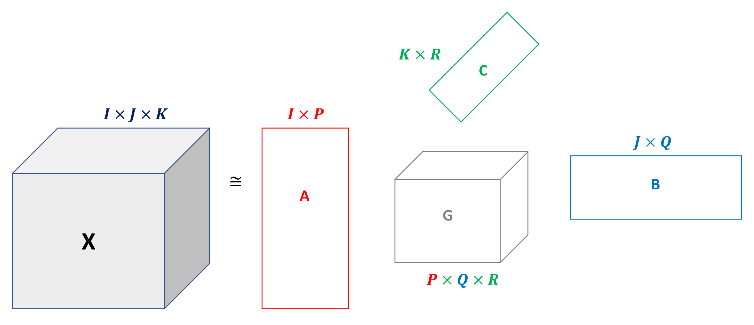
3.3. Three-Way Analysis

Data are organized in a three-way array $\underline{\mathbf{X}}$, so that the element $x_{ijk}$ contains the ratio of passengers in the station i at time j on day k. It is important to notice that three-way models need the number of variables to be the same each day. For this reason, only those hours in which all stations are open every day, i.e., 5:00 to 24:00, are studied.

The model chosen for the analysis of these data was the Tucker3 model, as it was considered that the number of components for each mode could be different. The R package ThreeWay [38] was used for data analysis.

Tucker3 analysis was performed on the dataset for all valid ranks between $(1,1,1)$ and $(5,5,5)$. In order to select between the many estimated models a solution that optimally balances model fit and model complexity, the CHull model selection procedure was applied [34,36] with the fit percentages and the total number of fitted components (i.e., $P+Q+R$) as complexity value. The best solutions found were those located along the higher boundary of the convex hull. These solutions, together with the corresponding $st$-values, are shown in

Table 2. Best solutions according to the CHull procedure.

(P, Q, R)	P + Q + R	Fit	St Ratio
$(1,1,1)$	3	86.76	−
$(2,2,2)$	6	94.22	1.06
$(2,3,2)$	7	95.04	8.78
$(3,4,2)$	9	95.82	1.67
$(5,5,4)$	14	96.85	0.92
$(5,5,5)$	15	96.93	−

.

Based on the CHull plot, shown in Figure 6, and the results presented in Table 2, it was decided to keep the $(2-3-2)$ solution, which has two components for stations, three components for hours, and two components for days.

This model explains $95.04\%$ of the data variance. It is important to notice how, by increasing the number of components, the performance improves (see Table 2); however, the interpretation of the model becomes more complex.

The rotational indeterminacy was used to reach the maximal simplicity for the core tensor and the component matrices in order to facilitate interpretation of the solution. The post-processed component matrices for timetable and days are given in

Table 3. Component matrix B for timetable (with values exceeding $0.20$ in absolute value indicated in bold).

Timetable	Component 1	Component 2	Component 3
5 a.m.	$-0.06$	0.12	0.05
6 a.m.	0.12	0.18	0.18
7 a.m.	0.06	0.01	0.62
8 a.m.	0.05	0.07	0.68
9 a.m.	$-0.02$	0.25	0.29
10 a.m.	$-0.09$	0.49	0.00
11 a.m.	$-0.06$	0.51	−0.04
12 a.m.	0.03	0.41	−0.06
1 p.m.	0.19	0.27	−0.03
2 p.m.	0.37	0.00	0.06
3 p.m.	0.31	−0.02	0.10
4 p.m.	0.14	0.26	0.03
5 p.m.	0.40	−0.01	0.06
6 p.m.	0.56	−0.13	0.00
7 p.m.	0.33	0.10	−0.04
8 p.m.	0.24	0.14	−0.05
9 p.m.	0.17	0.11	−0.05
10 p.m.	0.09	0.09	−0.05
11 p.m.	0.08	0.07	−0.05

and

Table 4. Component matrix C for days of the week. (Note: component scores higher than 0.20 in absolute value are in bold).

Day	Component 1	Component 2
Monday	−0.05	0.47
Tuesday	−0.04	0.47
Wednesday	−0.02	0.45
Thursday	0.03	0.42
Friday	0.02	0.42
Saturday	0.63	0.05
Sunday	0.77	0.00

. The post-processed core array is presented in

Table 5. Core array from Tucker3 analysis with P= 2, Q= 3, and R= 2 components for the dataset (with values exceeding $1.5$ in absolute value being indicated in bold and values exceeding 3 in absolute value being underlined).

	Day Component 1			Day Component 2
Station Comp.	Hour C1	Hour C2	Hour C3	Hour C1	Hour C2	Hour C3
1	1.94	2.07	0.77	2.67	2.52	3.89
2	1.62	1.44	0.33	3.36	1.87	1.11

. Note that the core array is presented as a matrix where rows represent the stations components and columns represent the combination of hours and days components. Part of the station component matrix, which is not shown in full because of its excessive length, can be found in

Table 6. Component matrix A for selected stations.

Station	Component 1	Component 2
Roquetes	0.17	−0.08
Santa Rosa	0.17	−0.08
La Salut	0.15	−0.05
Llefià	0.15	−0.06
Trinitat Nova	0.15	−0.05
Can Cuiàs	0.14	−0.03
Can Peixauet	0.14	−0.04
Canyelles	0.14	−0.04
Ciutat Meridiana	0.14	−0.04
Pep Ventura	0.14	−0.04
Fira	−0.05	0.22
Mas Blau	−0.05	0.21
Parc Logístic	−0.05	0.21
Palau Reial	−0.03	0.19
Ciutadella	−0.03	0.17
Hospital de Bellvitge	−0.02	0.17
Maria Cristina	−0.01	0.17
Mercabarna	−0.02	0.17
Diagonal	−0.01	0.16
Drassanes	−0.01	0.16
Alfons X	0.08	0.05
Av.Carrilet	0.08	0.04
Clot	0.08	0.04
Bellvitge	0.07	0.05
Collblanc	0.08	0.04
Encants	0.08	0.04
Fabra i Puig	0.07	0.05
Hospital de Sant Pau	0.06	0.07
Joanic	0.06	0.06
Poblenou	0.07	0.06

. Stations with high loads in the first component appear in the first block of the table, those with high loads in the second component appear in the second block, and finally in the third block those with high loads in both components.

To evaluate the results obtained, the three component matrices were inspected so that if an element has high value (in an absolute sense) on a component it is interpreted as playing an important role in the corresponding component.

As previously noted, the time information is described in terms of the different loadings for each hour on the three components of the second mode (Figure 7, Figure 8 and Figure 9). In Table 3, it can be seen that Component 1 for the timetable mainly depends on 14:00, 15:00, 17:00, 18:00, 19:00, and 20:00. Hence, this component can be associated with afternoon and evening peak hours. Component 2 is strongly related to 10:00, 11:00, and 12:00, and so this component could be defined as off-peak hours. Finally, Component 3 has high values on 7:00 and 8:00 so it could be interpreted as morning rush hour. Some hours present high loads in more than one component, e.g., 9:00, with high loads on the second and third components.

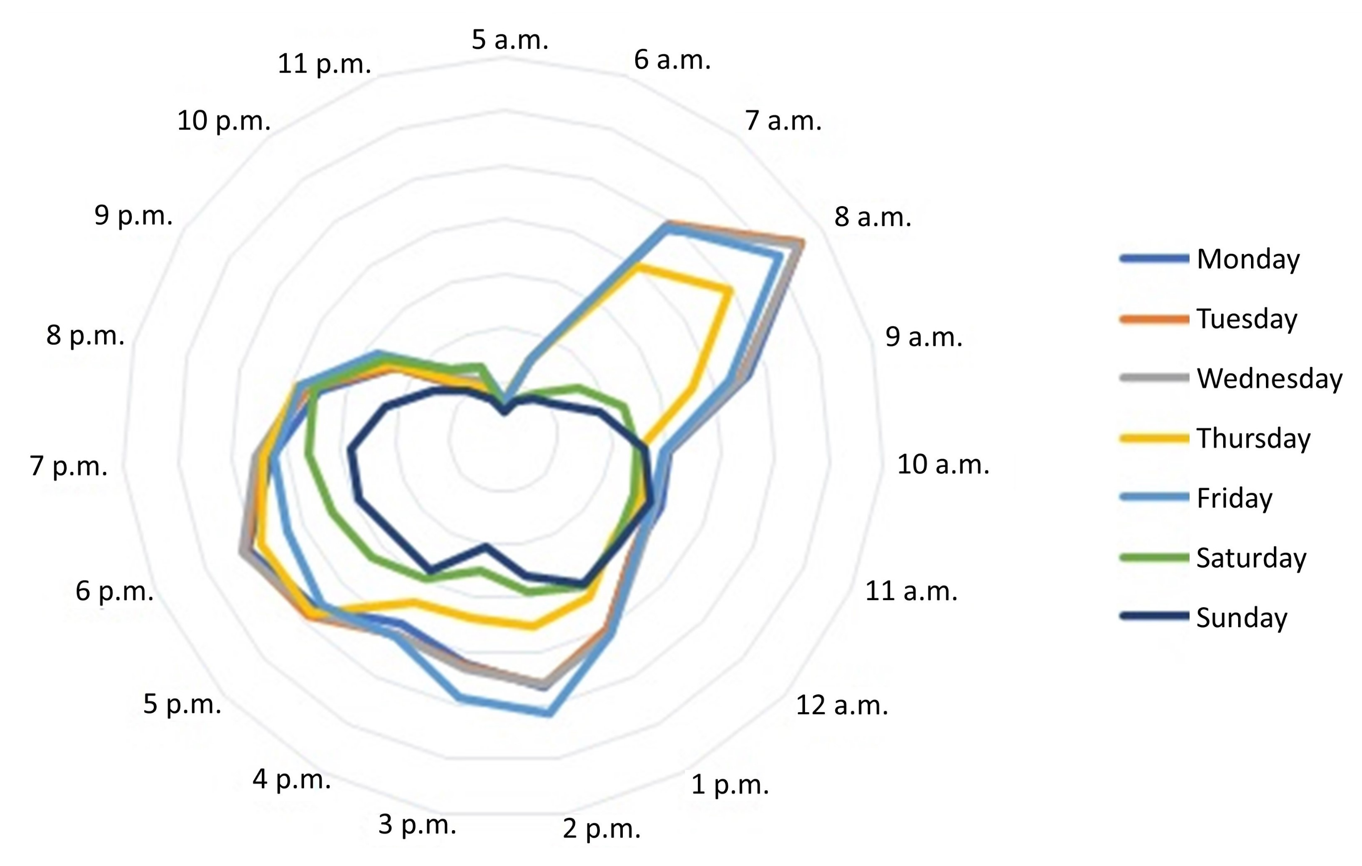
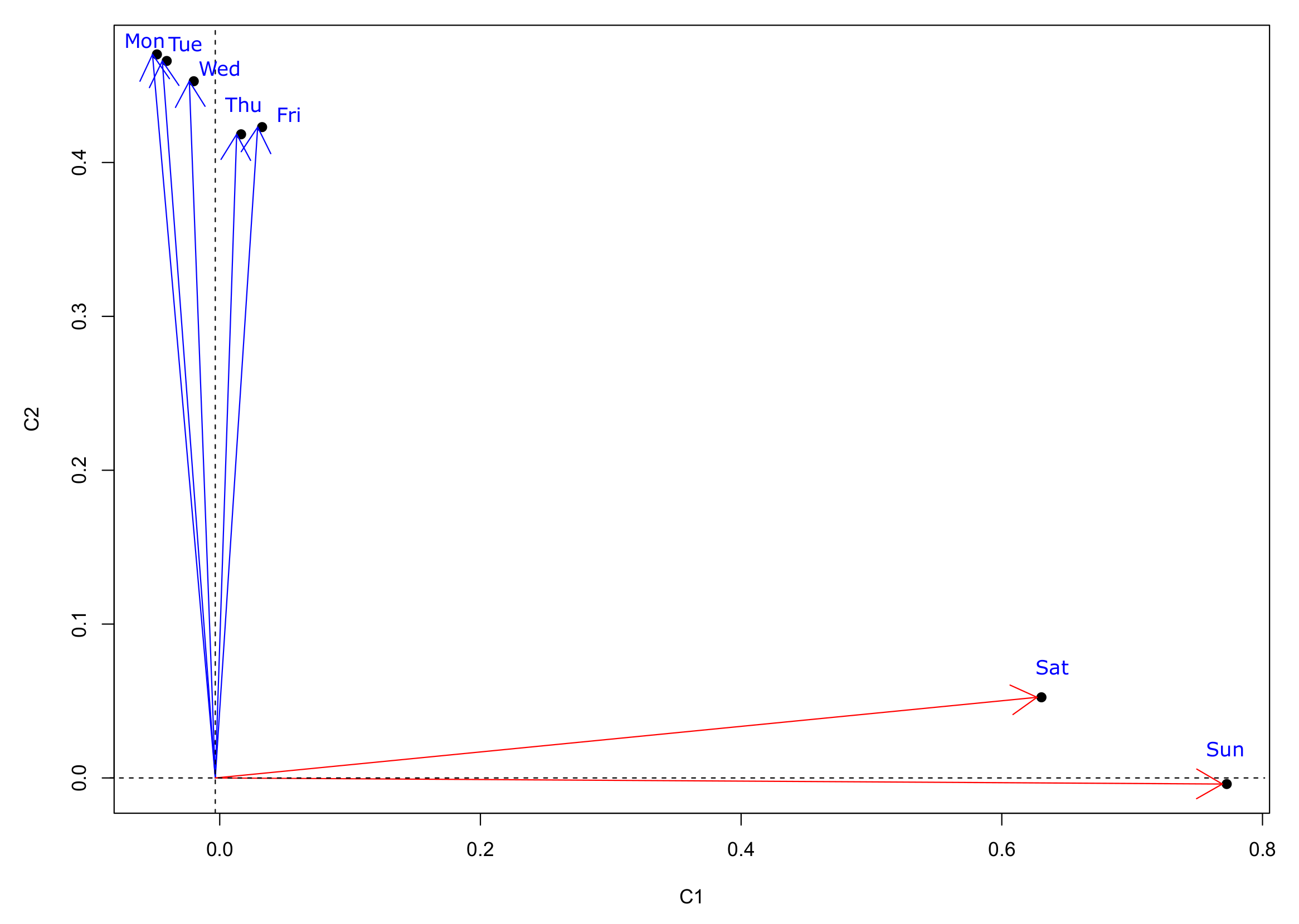
When inspecting the day component matrix (see Table 4 and Figure 10), it can be noted that the first component refers to weekend days and the second component clearly refers to weekdays, as Saturday and Sunday load high on the first component and the rest of the days on the second one.

The station scores (shown for prototypical stations in Table 6) indicate the position of each station on these dimensions. When discarding small station scores, most stations have high loadings on one dimension and a few on both dimensions. It is important to note that the stations that score high in one component score negatively in the other one. For example, Roquetes and Santa Rosa are the stations with the highest loading on the first dimension, Fira and Mas Blau the stations with the highest loading on the second dimension, and Poblenou and Hospital de Sant Pau load high on both dimensions. Therefore, three clusters of stations can be considered. The stations belonging to each cluster are shown in

Table 7. Results of station classification.

Cluster	Stations	Number
Cluster 1	Aeroport T1, Aeroport T2, Arc de Triomf, Barceloneta, Bogatell, Catalunya, Ciutadella, Diagonal, Drassanes, El Maresme-Fórum, Entença, Europa-Fira, Fira, Fontana, Girona, Gloriès, Hospital Cliníc, Hospital de Bellvitge, Jaume I, Lesseps, Liceu, LLacuna, Maria Cristina, Marina, Mas Blau, Mercabarna, Mundet, Palau Reial, Parc Logístic, Passeig de Gràcia, Sagrada Familia, Selva de Mar, Tetuan, Universitat, Urquinaona, Vall d’Hebron, Verdaguer, Verneda, Zona Universitària	39
Cluster 2	Artigues, Badalona-Pompeu Fabra, Besòs, Besòs Mar, Camp de l’arpa, Can Boixeres, Can Cuiós, Can Peixauet, Can Serra, Can Vidalet, Can Zam, Canyelles, Cèntric, Ciutat Meridiana, Congrés, El Carmel, El Coll-La Teixonera, El Prat Estació, Església Major, Florida, Fondo, Gavarra, Gorg, La Pau, La Salut, Llefià, Llucmajor, Maragall, Mercat Nou, Pep Ventura, Pubilla Cases, Roquetes, Sagrera, Sant Ildefons, Sant Martí, Santa Coloma, Santa Rosa, Singuerlín, Torrassa, Torre Baró, Trinitat Nova, Trinitat Vella, Valldaura, Via Júlia, Vilapicina, Virrei Amat	46
Cluster 3	Alfons X, Av. Carrilet, Bac de roda, Badal, Baró de viver, Bellvitge, Bon pastor, Can tries-Gornal, Casa de l’aigua, Clot, Collblanc, Cornellà Centre, Encants, Espanya, Fabra I Puig, Guinardó, Horta, Hospital de Sant Pau, Hostafrancs, Joanic, Les Corts, Les Moreres, Montbau, Monumental, Navas, Onze De Setembre, Parallel, Parc Nou, Penitents, Plaça De Sants, Plaça Del Centre, Poble Sec, Poblenou, Rbla. Just Oliveras, Rocafort, Sant Andreu, Sant Antoni, Sant Roc, Santa Eulàlia, Sants Estació, Tarragona, Torras I Bages, Urgell, Vallcarca	44

. Cluster 1 is formed by stations that have a high score on the second dimension, cluster 2 by those with high scores on the first dimension, and, finally, cluster 3 by the stations that have high scores in both dimensions. To ease the interpretation of the results, spatial location of the clusters within the Barcelona metro network is shown in Figure 11, where Voronoi diagrams (based on Euclidean distance) are used, so that each cell represents a station that is coloured according to the cluster it belongs to.

Cluster 1 includes, amongst others, stations located in the industrial and logistics zones of the city (Fira, Mas Blau, MercaBarna, and Parc Logístic), hospitals ( Hospital Clínic, Hospital de Bellvitge, and Vall D’Hebron), and those belonging to the University campus (Zona Univesitá, Marina, Universitat, Ciutadella, and Diagonal). In addtion, stations close to hotels and landmarks are included, such as Sagrada Família, El Born, Barceloneta, Plaza Catalunya, Passeig de Gràcia, Jardines de Pedralbes, Barrio de Gràcia, Les Rambles, and Palau de la Música, among others. The two stations in Barcelona’s airport also belong to this group. Stations in cluster 2 are mainly located in the municipalities of Badalona, San Adriá de Besós, Hospitalet de LLobregat, Esplugas de LLobregat, El Prat de LLobregat, Cornellá de LLobregat, Moncada y Reixach, Santa Coloma de Gramanet, and some surrounding neighbourhoods such as Nou Barris and Sant Andreu. Finally, stations in cluster 3 are locate around the city center of Barcelona, mainly in Sant Andreu y Horta Guinardó.

Once the component matrices have been analyzed individually for each mode, a detailed analysis of the core array is necessary. The core array summarizes the main interactions in the data. Therefore, the largest (in absolute value) core values are examined to find the main interactions.

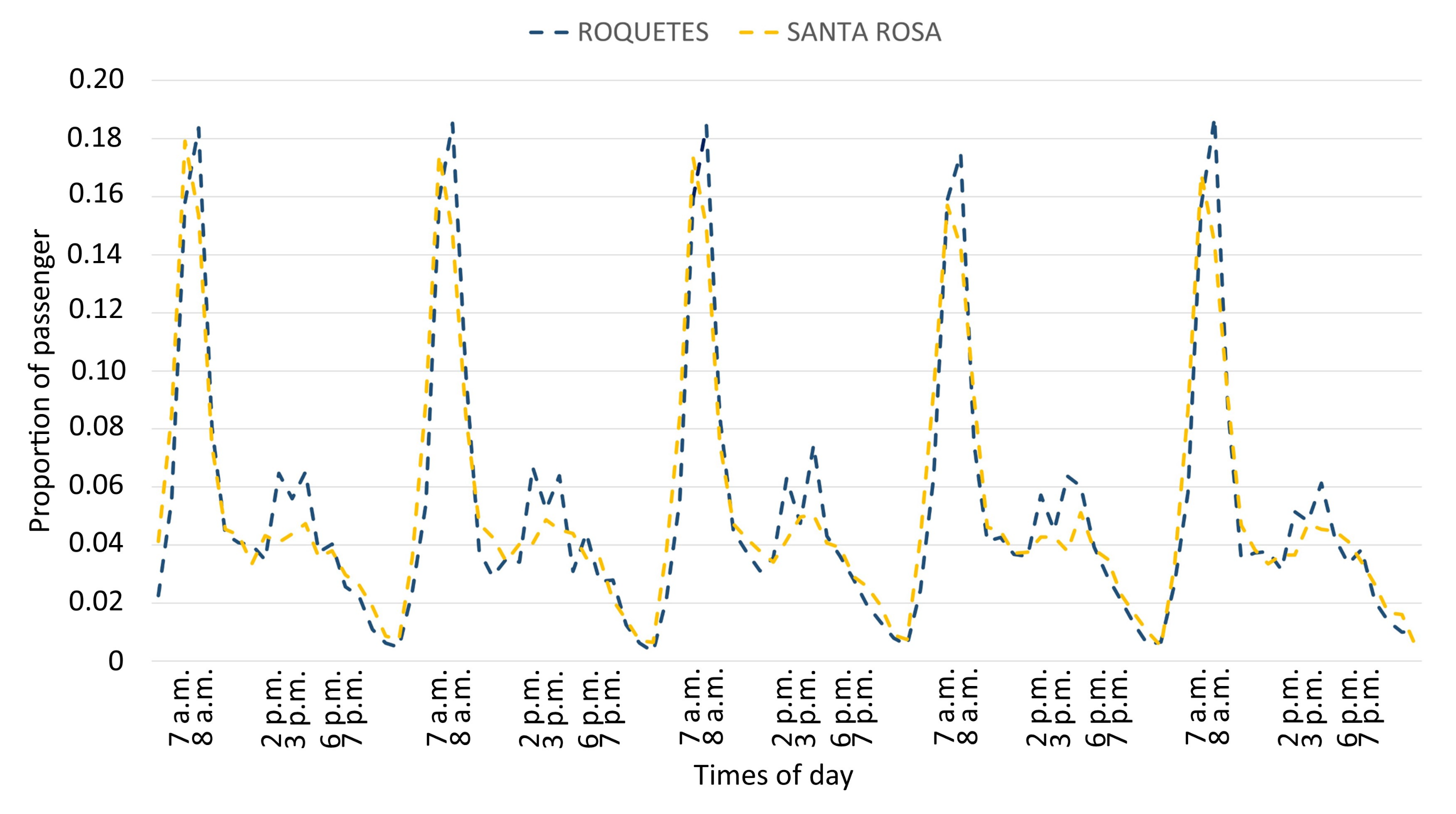
The core matrix $\underline{\mathbf{G}}$ indicates that the combination of components that extracts the largest variability is the combination of the first component of the first mode, the third component of the second mode, and the second component of the third mode, $g_{132}=3.89$ (Table 5). It indicates positive interaction among components P1, Q3, and R2. This reveals that stations with high loadings on the first component have an increase in the proportion of passengers when associated with the morning peak hours (7 a.m., 8 a.m.) on weekdays. This is the case of stations belonging to the Cluster 2 like Roquetes or Santa Rosa, amongst others. The passenger’s pattern of proportion per hour for Roquetes and Santa Rosa stations, both belonging to Cluster 2, is shown in Figure 12. In that figure, the highest passenger flow taking place between 7 and 8 in the morning is shown. In contrast, stations with negative values on the first component have a decrease in the proportion of passengers in the rush hours in the morning (Figure 13).

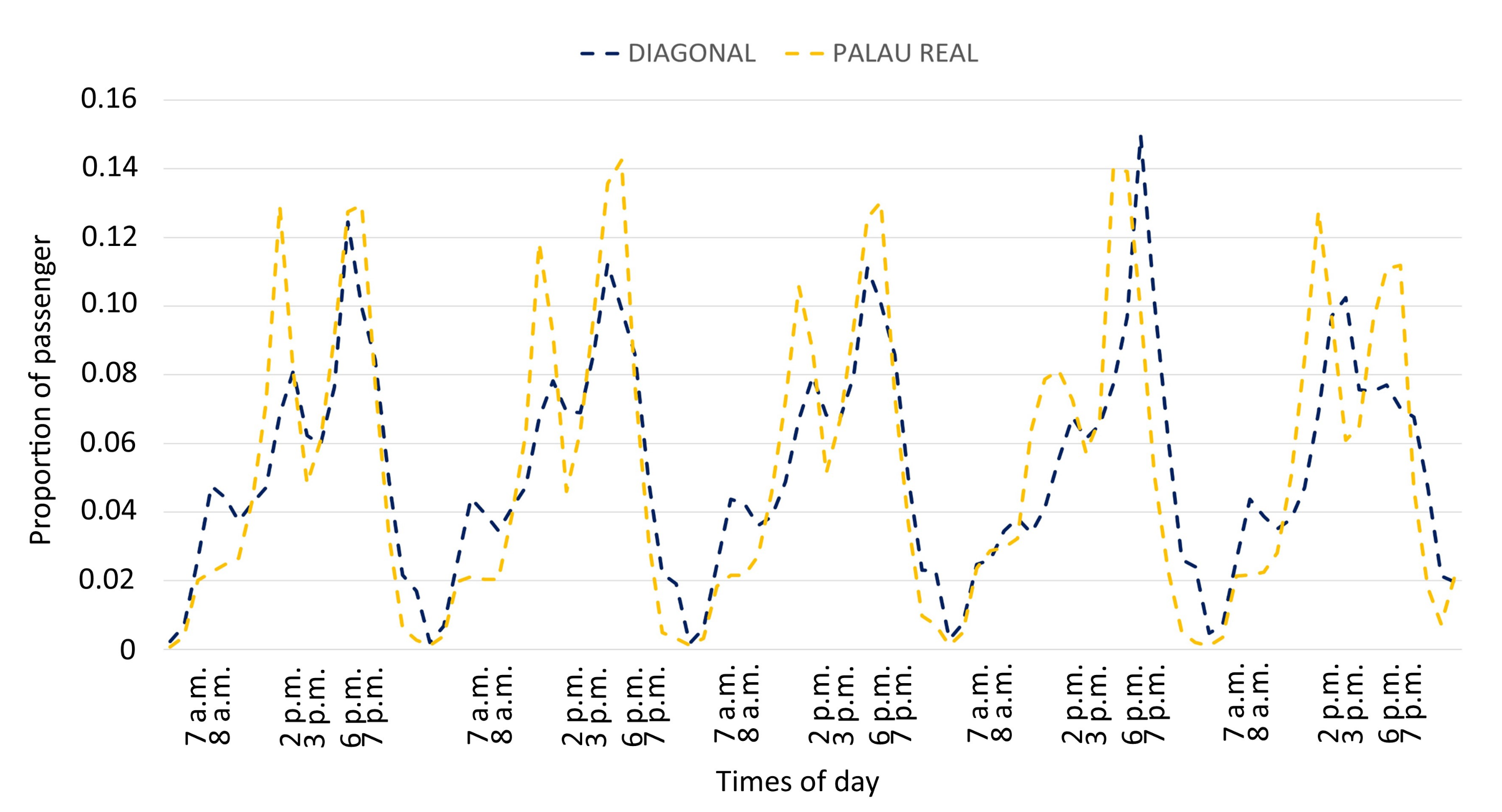
The core element $g_{211}=3.36$ among components P2, Q1, and R1 highlights that stations with high loading in the second component have a larger proportion of passengers in the afternoon and evening rush hours on weekdays. This is the case of stations in Cluster 1. In Figure 13, the pattern of proportion of passengers per hour is shown for Diagonal and Palau Real stations. According to the figure, the highest passenger flow takes place between 2 and 3 in the afternoon and 5 and 8 in the evening. It can also be seen how the stations in cluster 2 (with negative scores on the second component) have a lower proportion of passenger at peak hours in the afternoon and evening on weekdays (Figure 12).

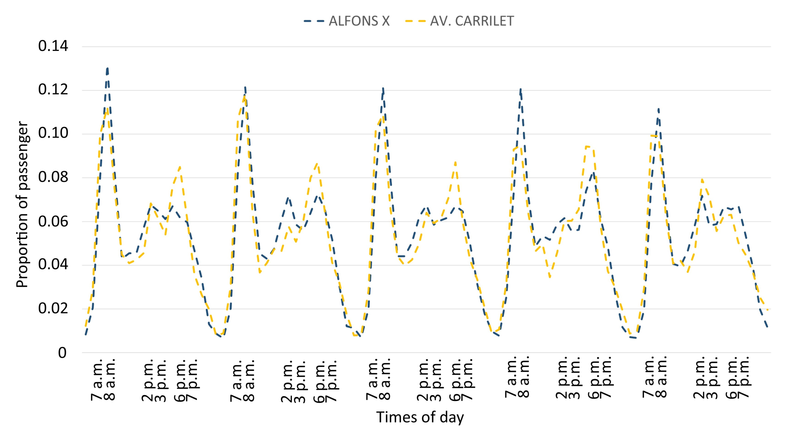
In contrast, as previously seen, there are stations with high loadings on both dimensions. Thus, in these stations there are peak hours both in the morning and in the afternoon on weekdays. Some stations in this group are Alfons X, Av.Carrilet, Clot, Bellvitge, Collblanc, Encants, Fabra i Puig, Hospital de Sant Pau, Joanic, and Poblenou. Figure 14 shows the pattern of proportion of passengers per hour for some stations in this group.

It is important to notice that the core elements related to the first component of the third mode (weekend days) take values below one on the third component of timetable (morning rush hour) ($g_{131}=0.77$ and $g_{231}=0.33$). This means there is no rush hour in the morning on weekends. Furthermore, the highest value in the core elements related to weekend days is $g_{121}=2.07$, therefore the greatest interaction occurs between the stations with high values on the first component during off-peak hours. Interaction with the first component of timetable (afternoon and evening rush hour) is quite similar in all stations ($g_{111}=1.94$ and $g_{211}=1.62$).

4. Conclusions

The aim of this work was to analyze the Barcelona metro network to discover its space-time structure. Previous studies relied on classical methods, such as PCA or clustering techniques. For instance, in [30] principal component analysis (PCA) is employed to reduce the number of variables and then, from the coordinates of the components obtained, a K-means clustering [39] is performed. With this approach, a classification of stations is obtained, but the temporal patterns that identify each group are not identified. The approach presented in this paper uses a three-way tensor (station of origin-day-time) to analyze the data from smart cards so that the original structure of the data can be respected. Moreover, multivariate analysis techniques have been applied to analyze the data; more specifically, the Tucker3 method was employed. As a result, three matrices were obtained (one for each mode), known as component matrices, and a core matrix. Through these component matrices, clusters of stations (stations that behave in a similar way in the dynamics of the metro network) and temporal patterns could be established. The core matrix has been used to model the relationships between the stations and the temporal patterns.

The results obtained show the efficiency of the Tucker3 method to analyze transport data and discover mobility patterns. It provides improvements in the clustering of stations in comparison to classical clustering methods commonly used in this type of data. The applied methodology allows the identification of daily patterns that separates weekdays from weekends. Three temporal patterns are also detected, corresponding to morning peak hours, off peak hours, and afternoon-evening peaks. Three spatial patterns are observed on working days. There are stations with morning peak hours (cluster 2 stations), others with afternoon and evening peak hours (cluster 1 stations), and the rest with both morning and afternoon peak hours (cluster 3 stations). No morning peak hours were observed on the weekends; the stations behave similarly and the hours with the highest passenger flow are in the morning.

The differences found with the results obtained in [30] highlight the improvement obtained by using Tucker’s method. It can be observed that the stations located in industrial and logistics areas, which formed an independent cluster in the previous study, are now all included in cluster 1, as the highest passenger flow in these stations occurs in the afternoon peak hours along with the rest of the cluster. Although it is true that, when comparing the clusters between the two methods, in one of the groups the coincidence reaches 76%, the changes in stations show that the behaviour of these stations, considering the neighbourhoods in which they are located, share more common characteristics in the clusters obtained by the Tucker method than using the classic conglomeration method.

The main disadvantage of this method is the difficulty in interpreting the results, as it is necessary to interpret the component matrices and the core matrix. Studies based on PARAFAC methods are easier to interpret because there is no core matrix, but they have a major drawback, which is that the number of components for all modes must be the same. Future lines of research may include the study of the relationship between station clusters and local environmental data, providing additional information for urban planning in the city in order to make decisions to improve the Barcelona metro network.