

Handling Irregular Many-Objective Optimization Problems via Performing Local Searches on External Archives


1
School of Electronic Engineering, Xidian University, Xi’an 710071, China
2
Inner Mongolia Institute of Dynamical Machinery, Hohhot 010010, China
3
School of Management, Hunan Institute of Engineering, Xiangtan 411104, China
*
Author to whom correspondence should be addressed.
Mathematics 2023, 11(1), 10; https://0-doi-org.brum.beds.ac.uk/10.3390/math11010010
Submission received: 23 October 2022
/
Revised: 8 December 2022
/
Accepted: 14 December 2022
/
Published: 20 December 2022
(This article belongs to the Special Issue Evolutionary Computation 2022)
Abstract
:Adaptive weight-vector adjustment has been explored to compensate for the weakness of the evolutionary many-objective algorithms based on decomposition in solving problems with irregular Pareto-optimal fronts. One essential issue is that the distribution of previously visited solutions likely mismatches the irregular Pareto-optimal front, and the weight vectors are misled towards inappropriate regions. The fact above motivated us to design a novel many-objective evolutionary algorithm by performing local searches on an external archive, namely, LSEA. Specifically, the LSEA contains a new selection mechanism without weight vectors to alleviate the adverse effects of inappropriate weight vectors, progressively improving both the convergence and diversity of the archive. The solutions in the archive also feed back the weight-vector adjustment. Moreover, the LSEA selects a solution with good diversity but relatively poor convergence from the archive and then perturbs the decision variables of the selected solution one by one to search for solutions with better diversity and convergence. At last, the LSEA is compared with five baseline algorithms in the context of 36 widely-used benchmarks with irregular Pareto-optimal fronts. The comparison results demonstrate the competitive performance of the LSEA, as it outperforms the five baselines on 22 benchmarks with respect to metric hypervolume.
Keywords:
evolutionary computation; many-objective optimization; irregular Pareto-optimal fronts; local search; external archiveMSC:
97M40; 97P301. Introduction
Optimization problems deriving from many fields often involve multiple conflicting objective functions. For example, scheduling workflows for cloud platforms needs to simultaneously minimize economical cost and completion time [1,2,3]. In general, reducing economical cost means renting cloud resources with lower configuration, thereby prolonging task execution time and workflow completion time. Thus, the two optimization objectives of scheduling cloud workflows conflict. In addition, accuracy and robustness are two conflicting objectives for neural-network-architecture searching [4]. These problems are termed multi-objective optimization problems (MOPs), which are mathematically formulated as:
where is the decision vector of n variables, and represents the objective vector of m objectives , . is the feasible search space. MOPs with more than three objectives, i.e., , are commonly termed many-objective optimization problems (MaOPs). Due to the conflicts between optimization objectives, no single solution can optimize multiple objectives simultaneously. Instead, there is a set of compromise solutions which is called the Pareto-optimal solution set in the decision space and the Pareto-optimal front in the objective space.
With the attractive feature of creating a set of solutions in each iteration, evolutionary algorithms have been intensively explored to resolve MaOPs. Over the past two decades, researchers and engineers have proposed and developed numerous evolutionary many-objective optimization algorithms (EMOAs) to resolve MaOPs from various domains [5,6,7,8]. According to the environmental selection framework, most of the established EMOAs can be roughly classified into three categories: Pareto-dominance-based, indicator-based, and decomposition-based EMOAs. Regarding the algorithms based on Pareto dominance [9,10,11], they partition the combined population into different non-dominated levels (, , and so on). Then, solutions in each level are selected one at a time, starting from , until the number of selected solutions equals the population size or the time exceeds the pre-defined limit. Next, a secondary metric, e.g., crowding distance, is used to sort solutions in the last accepted level. The indicator-based EMOAs [8] attempt to quantify the population using one indicator, such as Hypervolume [12] or inverted generational distance [13]. For the EMOAs based on decomposition (EMOA/Ds) [14,15], they first employ Das and Dennis’s systematic approach [16] to initialize a set of uniformly-distributed weight vectors within a simplex, and then leverage these weight vectors to convert one single MaOP into a series of subproblems, which are solved in a cooperative way.
Among the three categories of EMOAs, the decomposition-based ones are commonly recognized as an effective way to solve MaOPs by substantially relieving selection-pressure-loss issues in Pareto-dominance-based EMOAs and the high computing overhead of calculating indicator values in indicator-based EMOAs [15]. The EMOA/Ds perform well on MaOPs with regular Pareto-optimal fronts, e.g., simplex-like shapes. However, they perform poorly on MaOPs with irregular Pareto-optimal fronts, such as discontinuous, degenerate, inverted, badly-scaled, or strongly concave/convex shapes [17,18,19]. In this case, some weight vectors cannot intersect with the Pareto-optimal fronts and become invalid, resulting in a waste of search resources allocated to these subproblems defined by the invalid weight vectors. Then, the capacity of EMOAs to solve MaOPs with irregular Pareto-optimal fronts deteriorated. For example, the RVEA and its variants [20,21], each solution is associated with a weight vector with the smallest acute angle, and at most one solution is reserved for a weight vector. For confronting the irregular Pareto-optimal fronts, some weight vectors of these algorithms are associated with multiple solutions, while many weight vectors are not associated with solutions [22,23]. This causes the weight vectors without associated solutions to become invalid, and the number of output solutions obtained by these algorithms is far less than the population size.
Researchers and engineers have recently tailored various algorithms to make a sound trade-off between convergence and diversity for EMOA/Ds in solving MaOPs with irregular Pareto-optimal fronts [17,24]. Most algorithms in this direction can be classified into the following three categories. In the first category, they adjust the distribution of weight vectors by using the solutions in the current population or archive. For instance, Li et al. explored the distribution of solutions in the archive for weight generation, weight addition, and weight deletion [25]. Liu et al. employed the objective vectors of solutions in the current population to adjust the weight vectors by adding angle thresholds [26]. Algorithms falling into the second category intend to learn the distribution of weight vectors by performing machine learning on visited solutions [27,28]. For instance, self-organizing mapping techniques and growing neural gas networks are employed to assist weight-vector adjustment [29,30,31]. For the above two categories of algorithms, the weight-vector adjustment depends on the distribution of visited solutions, which is often inconsistent with the irregular Pareto-optimal fronts. In this scenario, weight vectors will be misled into inappropriate areas, wasting computation resources. In the third category, the algorithm replaces inactive weight vectors by generating new ones. For instance, Jain et al. added new weight vectors around the active ones when the active number was less than the population size [32]. Cheng et al. suggested randomly generating additional weight vectors to compensate for invalid ones [20]. Elarbi et al. suggested adding multiple normal-boundary intersection directions to approximate irregular Pareto-optimal fronts [33]. However, facing the objective space of exponential growth, the weight vectors added by the third category of algorithms are likely ineffective.
In sum, the algorithms based on visited solutions mislead weight vectors to unsuitable areas, and algorithms that do not refer to visited solutions likely add ineffective weight vectors. Thus, adjusting the weight vectors for unknown shapes of irregular Pareto-optimal fronts is a dilemma. What is worse, when solving MaOPs with strongly convex or concave Pareto-optimal fronts, is the solutions do not inevitably converge to the intersection of the weight vectors and the Pareto-optimal fronts. This fact further challenges the EMOA/Ds to balance diversity and convergence.
To cope with the above-mentioned issues of the weight vector adjustment-based algorithms, this paper suggests adding an external archive, and presents a selection mechanism without weight vectors to maintain this archive. The core idea of this selection mechanism is to associate each new solution with a previously preserved solution with the minimum distance, and preserves the new solution only when it has better convergence and diversity than the associated solution. Moreover, it performs local searches on solutions with better diversity and relatively poor convergence to further strengthen convergence and diversity. Of course, the solutions in the archive also feed back the weight-vector adjustment.
2. Algorithm Design
This section designs a local search-assisted external archive mechanism to improve the EMOA/Ds using weight-vector adjustment to solve many-objective optimization problems with irregular Pareto-optimal fronts.
2.1. Main Framework of LSEA
The many-objective optimization problems with irregular Pareto-optimal fronts still pose challenges for the multi-objective evolutionary community. Although the weight-vector-adaptive adjustment can improve EMOA/Ds’ performance to a certain extent, the adjustment of the weight vectors heavily depends on the visited solutions, unexpectedly misleading the weight vectors to unsuitable search areas. Considering this, we propose a novel many-objective evolutionary algorithm by performing local searches on an external archive. This algorithm embraces an external archive to maintain a well-converged and well-distributed population, and further strengthens convergence and diversity by conducting local searches on solutions with better diversity and relatively poor convergence. Its main framework is summarized as Algorithm 1.
As shown in Algorithm 1, the pivotal inputs of the LSEA are an optimization problem, the population size, and the termination condition. With the above inputs, the LSEA begins with initializing a set of weight vectors (Line 1) and the neighborhood of each weight vector (Line 2). records the indexes of the T closest weight vectors of the i-th weight vector, where T refers to the number of the weight vectors in the neighborhood. If , the b-th subproblem is termed as a neighbor of the i-th subproblem. Then, it randomly generates N solutions to construct the initial population P and the external archive (Lines 3–4). Additionally, the number of used evaluation times and the ideal point are updated (Lines 5–6).
The LSEA follows the mainstream framework of the EMOA/Ds using weight-vector adjustment. Its main loop includes offspring population generation, weight-vector adjustment, and maintenance of the external archive.
| Algorithm 1: Main framework of LSEA. |
 |
Before the offspring population generation, a set Q is initialized to record the offspring solutions (Line 8). Then, the subproblems are iterated one by one to generate new solutions (Line 9). In this process, the solutions belonging to each subproblem and its neighborhood are randomly selected, and an existing variation operator, such as differential evolution [34,35], cuckoo search [36,37], or krill herd optimization [38], is used on these selected solutions. Then, the number of used evaluation times and the ideal point are updated (Lines 11–12). After that, the new solution will be used to update the solutions belonging to the i-th subproblem and its neighborhood (Lines 13–15). If the fitness of is better than that of compared solutions (Line 14), it will replace them. Note that and , respectively, represent the solution and weight vector corresponding to the b-th subproblem. The EMOA/D and its variants generally calculate the fitness of a solution using the following three approaches [15]: penalty-based boundary intersection, weighted sum, and Tchebycheff. Among them, the Tchebycheff-based approach is more prevalent in solving many-objective optimization problems [39,40]. The Tchebycheff value of solution to weight vector can be calculated as:
where is the ideal point and indicates the i-th weight vector.
For the weight-vector adjustment approach (Line 17), designing a new one is not the focus of this paper. We directly use the growing neural gas network-based weight-vector adjustment approach [30]. In this approach, the growing neural gas network is employed to dynamically learn the topological structures of the irregular Pareto-optimal fronts. Then, the nodes of the growing neural gas network are adopted to adjust the weight vectors.
For maintaining the external archive, all the new solutions in this iteration are employed to update the external archive (Line 18), which is summarized in Algorithm 2. After the LSEA meets the termination condition, it outputs the external archive .
2.2. Maintain External Archive
Adjusting weight vectors based on the visited solutions is a promising way to compensate for EMOA/Ds’ deficiency in solving MaOPs with irregular Pareto-optimal fronts. Unfortunately, the distribution of obtained solutions often cannot well approximate the irregular Pareto-optimal fronts, especially in the early stage of the evolutionary search. In this scenario, the weight vectors are always misled to the unsuitable search area, which will seriously inhibit the potential of the EMOA/Ds to balance diversity and convergence. To address the aforementioned issue, this paper designs a new selection mechanism without weight vectors to maintain a well-converged and well-diversified external archive. Moreover, the proposed algorithm performs local searches on solutions with good diversity but relatively poor convergence to further strengthen convergence and diversity. The main steps of Function MaintainExternalArchive() is summarized in Algorithm 2. Before detailing this function, we define the convergence and diversity for solutions as follows.
The -metric is employed to evaluate the convergence of solutions, which is calculated as follows.
Relative to population P, the diversity of a solution is defined as:
As illustrated in Algorithm 2, the primary inputs of Function MaintainExternal Archive() are: the archive, a new population, the population size, and the ideal point. This function can be roughly divided into two stages: environmental selection and local search.
The first stage strives to maintain a well-converged and well-diversified archive as follows. The dominated solutions in the combined population are first removed (Line 1) to ensure that only non-dominated solutions are retained in the archive. Then, the non-dominated solutions in the archive and the offspring population are selected (Lines 2–3). After that, if the number of solutions in the archive is less than the population size (Line 4), then the solution with the minimum ratio of convergence to diversity (Line 8) is moved from Q to one by one until the population size is reached or the set Q become empty. Next, each remaining solution in the Q will be associated with a solution with the minimum distance (Line 15), which is defined in (4). These two solutions will compete for survival. If the remaining solution in the Q is better than the associated solution with respect to both convergence and diversity (Line 16), it will replace the associated solution (Lines 17–18).
The second stage (Lines 19–25) attempts to perform local searches on solutions with good diversity but relatively poor convergence, avoiding the elimination of solutions with better diversity due to insufficient convergence. During this stage, a solution is first selected from the archive by applying roulette-wheel selection based on the sum of diversity and convergence values, which are, respectively, defined in (5) and (3) (Line 19). Note that the symbol n in line 21 denotes the number of decision variables. Afterward, all decision variables of the selected solution are perturbed one by one to reproduce new solutions (Line 22). If a new solution is better than the previous solution with respect to both convergence and diversity (Line 23), the new solution will be retained (Line 24).
| Algorithm 2: Function MaintainExternalArchive(). |
 |
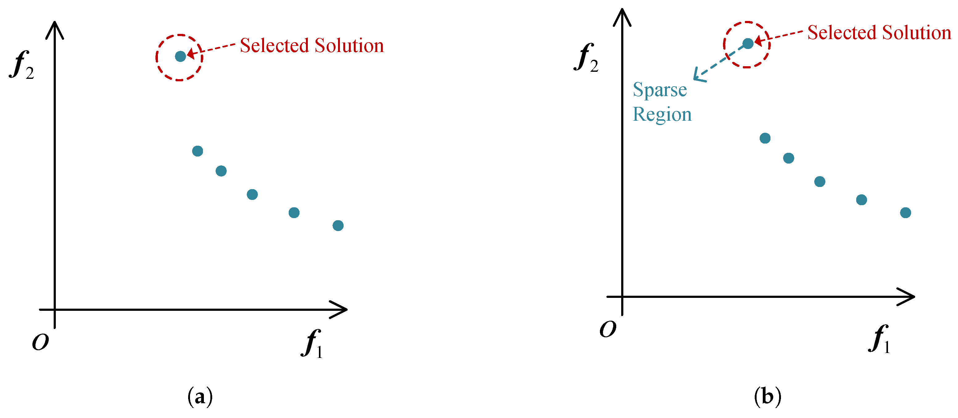
Figure 1 provides an illustrative example to explain the local searches for a solution with good diversity but relatively poor convergence. In Figure 1, each solid blue point corresponds to a solution. We can observe that the solution within the red circle poses good diversity; that is, it is in a sparse region. However, its convergence is relatively poor, and it is likely to be discarded when it is dominated by the offsprings of better-converged solutions. Based on the policy of the local search, it will select this solution and perturbs all decision variables one by one to reproduce new solutions to explore the sparse region. This way, both the diversity and convergence of the population are strengthened.
3. Experimental Studies
This section provides the experimental settings and analyzes the comparison results to verify the performance of the proposed LSEA.
3.1. Experimental Settings
Competitors: Five existing EMOAs, i.e., MOEA/D-CWV [44], DEA-GNG [30], MaOEA/IGD [13], NSGA-III [45], and MOEA/D-PaS [46], are chosen for comparison experiments. For these five baseline EMOAs, they were implemented on MATLAB and exposed to the platform PlatEMO 3.4 [47]. Unless otherwise specified, these baseline EMOAs directly adopt the defaulted parameter settings in the platform.
Benchmark functions: Cheng et al. [48] designed the test suite MaF1–MaF15 by considering various characteristics of real-world applications, e.g., irregular Pareto-optimal fronts, complex landscapes, and large-scale decision variables. In detail, the functions MaF1–MaF9 have irregular Pareto-optimal front shapes, and the other functions mainly reflect the characteristics of MaOPs with complex Pareto sets and large-scale decision variables. Since this paper tries to resolve MaOPs with irregular Pareto-optimal fronts, we selected functions MaF1–MaF9 to perform the experiments and set the number of optimization objectives for the selected functions as 5, 10, 13, and 15, respectively. After configuring a benchmark function with a specific objective number, we term it a test instance, e.g., 10-objective MaF1.
Population Size: For fairness, the population size of the six algorithms is set according to the number of optimization objectives. Specifically, they are 210, 230, 182, and 240 for optimization problems with 5, 10, 13, and 15 objectives, respectively.
Termination Condition: Similar to published papers [30,49,50], we resorted to the maximum number of function evaluations as the termination condition and set it to for each test instance.
Performance Metrics: The hypervolume (HV) [51] and inverted generational distance (IGD) [52] are two common metrics for assessing the quality of a solution set concerning convergence and diversity. In the experiment, they were employed to measure the quality of solution sets obtained by the six algorithms.
- (1)
- The metric HV represents the volume of space composed of a reference vector and a non-dominated solution set in the objective space. Assuming that the reference vector is and the solution set is P, the HV value of P can be estimated as below:where refers to the Lebesgue measure. In the experiments, the reference vector of a test instance is set as 1.5 times its nadir point. According to (6), it can be derived that a larger HV value of a solution set implies the corresponding algorithm being better in both convergence and diversity.
- (2)
- Suppose is a set of vectors evenly distributed over the Pareto-optimal front of an MaOP. The IGD value of a solution set P can be estimated as below:where refers to the Euclidean distance between vector and objective vector of solution . According to (7), it can be derived that the solution set with a smaller value implies the corresponding algorithm being better in both convergence and diversity. In the experiments, around 40,000 vectors are evenly sampled from the Pareto-optimal front of each test instance.
In each test instance, the six algorithms were repeated 30 times, and their average values and standard deviation for the two metrics are reported. The best average value is highlighted with a gray background. In addition, the Wilcoxon rank-sum test with a significance of 5% was employed to identify the significant difference between the LSEA and each competitor. The signs −, +, and ≈ indicate that the competitor performs significantly worse, better, and similarly to the LSEA, respectively.
All the experiments were conducted on a workstation, which was Windows Server 2016, 256 GB RAM, and Intel(R) Gold 6226R CPUs.
3.2. Experimental Results and Analysis
With respect to metric HV, Table 1 summarizes the comparison results of the six algorithms, i.e., MOEA/D-CWV, DEA-GNG, MaOEA/IGD, NSGA-III, MOEA/D-PaS, and LSEA, on the thirty-six test instances (MaF1–MaF9 with 5, 10, 13, and 15 objectives). In addition, a triple in the last row of this table represents the number of test instances that the corresponding baseline is significantly inferior to, significantly superior to, and similar to the LSEA. For example, the triple in Table 1 represents that the MOEA/D-CWV is significantly inferior to the LSEA in 25 test instances, significantly superior to the LSEA in 6 test instances, and similar to the LSEA in 5 test instances.
The experimental results in Table 1 illustrate that LSEA has strong competitiveness in solving MaOPs with irregular Pareto-optimal fronts, as it performed best on 22 out of 36 test instances by metric HV. By comparison, MOEA/D-CWV, DEA-GNG, MaOEA/IGD, NSGA-III, and MOEA/D-PaS, respectively, performed best in 0, 3, 0, 11, and 0 instances for metric HV. In addition, the LSEA was significantly superior in MaF1, MaF3, MaF6, MaF8, and MaF9 by all considered objective measures. These comparison results illustrate that the proposed LSEA substantially improved over the five baselines in resolving MaOPs with inverted, concave, disconnected, and degenerate Pareto-optimal fronts.
Although the proposed LSEA and the DEA-GNG all update the weight vectors according to the distribution of visited solutions learned by a growing neural gas network, the LSEA outperforms the DEA-GNG in most test instances. Unlike the DEA-GNG, the LSEA embodies a heuristic selection mechanism and a local search to maintain a well-converged and well-diversified archive, which also feeds back the weight-vector adjustment. The comparison results between LSEA and DEA-GNG show that the proposed mechanism in this paper has superior performance in resolving irregular Pareto-optimal fronts. In particular, the selection mechanism for the external archive in the LSEA only preserves these solutions with better convergence and diversity, effectively avoiding the adverse effects of inappropriate weight vectors. In addition, the local search for solutions with better diversity and relatively poor convergence is conducive to further strengthening convergence and diversity.
The MOEA/D-CWV is a recent weight-vector adjustment approach that dynamically adopts the intermediate objective vectors of the visited solutions to control the distribution of the weight vectors. Its HV values on 35 out of 36 test instances are significantly inferior to those of the proposed LSEA. One essential reason is that the distribution of the visited solutions being inconsistent with the Pareto-optimal fronts misleads the weight vectors to unsuitable areas, which unavoidably impairs the capability of MOEA/D-CWV in balance convergence and diversity. In the LSEA, the non-weight-vector selection mechanism for maintaining archives can alleviate the above drawbacks.
The NSGA-III is a classical baseline integrating Pareto-dominance-based and weight-vector-based environmental selection mechanisms. The HV values obtained by NSGA-III on 25 out of 36 test instances are lower than those of LSEA. The victory of NSGA-III over LSEA on test instances derived from badly-scaled MaF4 and MaF5. The primary reason is that the NSGA-III employs a hyperplane-based normalization procedure to obtain the intercepts along each objective dimension, mitigating the adverse effects of badly-scales among different objectives of MaF4 and MaF5. For MaOPs with other types of Pareto-optimal fronts, the proposed LSEA has strong advantages. Compared with MaOEA/IGD and MOEA/D-PaS, the LSEA poses an overwhelming advantage, as it performed significantly better than them on 30 out of 36 test instances; the MOEA/D-PaS significantly outperformed the LSEA on five test instances derived from MaF5.
It is reasonable to conclude that the proposed LSEA has a superior overall performance than MOEA/D-CWV, DEA-GNG, MaOEA/IGD, NSGA-III, and MOEA/D-PaS with respect to the metric HV. When compared to the five baselines, the main contribution of LSEA is to add an external archive to preserve solutions with better diversity and convergence, gradually approximating the Pareto-optimal fronts. The superior overall performance of LSEA on these 36 test instances demonstrates the effectiveness of the proposed mechanism in solving MaOPs with various Pareto-optimal fronts.
Regarding the metric IGD, the average values and standard deviations of the six algorithms on 5-, 10-, 13-, and 15-objective test instances are summarized in Table 2. By comparing the proposed LESA with the five baselines one by one, we can see that the LESA yielded significantly lower IGD values than MOEA/D-CWV, DEA-GNG, MaOEA/IGD, NSGA-III, and MOEA/D-PaS on 35, 23, 34, 25, and 32 out of the 36 test instances, respectively. These results again illustrate the superior performance of the proposed method in handling MaOPs with various Pareto-optimal fronts. By comparing the results between metrics HV and IGD, we can see that there exist differences in the ordering of the six algorithms. Take the 5-objective MaF1 as an example. The LSEA is significantly better than the DEA-GNG with respect to the metric HV, whereas the opposite is true with respect to the metric IGD. Although both metrics, HV and IGD, can simultaneously reflect the convergence and diversity of a solution set, their calculation methods are quite different. Specifically, the metric HV is compatible with Pareto dominance—i.e., the comparison result between two solution sets is always consistent with the Pareto-domination-based comparison result—whereas the metric IGD is not.
To intuitively compare the LSEA with the five baselines, we resort to the parallel coordinates plot [53] to illustrate their populations with the median HV values among 30 runs on 10-objective MaF1, MaF6, and MaF8, as shown in Figure 2, Figure 3 and Figure 4. The parallel coordinates plot maps m-dimensional vectors in a 2-dimensional graph with m parallel axes. The value of each dimension of a vector is converted to the vertices on the corresponding axis, and then a polyline connecting these m vertices represents this vector. Generally, a population is considered to have well convergence if it falls within the range of the Pareto-optimal front in the parallel coordinates plot. A population is considered to have good diversity if it spreads over the whole range of the Pareto-optimal front in the parallel coordinates plot.
The 10-objective MaF1 is the representative of MaOPs with inverted Pareto-optimal fronts. The value range of each dimension in 10-objective MaF1 is from 0 to 1. In Figure 2, the populations of the six algorithms fall in the range of 0 to 1, meaning they all have good convergence. This is because the landscape of MaF1 very simple, and it is easy to find the Pareto-optimal solutions. However, the inverted Pareto front of MaF1 brings difficulties to the environmental selection of EMOAs. For the baselines, MOEA/D-CWV, MaOEA/IGD, NSGA-III, and MOEA/D-PaS, the values in many objective dimensions are not less than 0.8, which means their diversity is poor. Among the five baselines, the DEA-GNG performed the best in both convergence and diversity. By comparing Figure 2b,f, we can observe that the DEA-GNG and the LSEA have good convergence, and the LSEA has much better diversity, especially for the first six objectives. The visual advantage of the LSEA concerning convergence and diversity in Figure 2 is consistent with its better metric values than the other five baselines.
The function MaF6 has a degenerate Pareto-optimal front. The lower bound of its Pareto-optimal front is 0 in each dimension, and the upper bounds in ten objectives are 4.0.0625, 0.0625, 0.0884, 0.1250, 0.1768, 0.2500, 0.3536, 0.5000, 0.7071, and 1.0, respectively. As illustrated in Figure 3, the values of most solutions obtained by DEA-GNG and NSGA-III on the ninth objective are far greater than 0.7071, or even as high as 240, meaning the output populations of these two baselines are far from converging to the Pareto-optimal front. Similarly, the MOEA/D-PaS is far from convergent on the tenth objective. Although MOEA/D-CWV and MaOEA/IGD exhibit good convergence, their output populations converged to very small areas, which means their diversity is very poor. Compared with the five baselines, the proposed LSEA poses outstanding performance in balancing convergence and diversity when solving MaOPs with degenerate Pareto-optimal fronts.
The function MaF8 is a classical Pareto-box problem whose Pareto-optimal domains are invariably 2D manifold in the decision spaces. The true Pareto-optimal solutions of MaF8 are evenly distributed within the polyhedron, as illustrated by the curves in Figure 4. From the distributions of the decision variables in Figure 4a, we can observe that the MOEA/D-CWV converges to one point outside the polygon, which means its poor convergence and diversity. As shown in Figure 4c,d, MaOEA/IGD, and NSGA-III pose good convergence by pushing all the solutions into the polygon. However, their diversity is poor, as the output solutions gather in a small area and do not evenly cover the interior of the polygon. The solutions obtained by MOEA/D-PaS are far from converging to the polyhedron. Compared with these five baselines, the proposed LSEA performs better in both convergence and diversity.
3.3. Performance Improvement of Local Search
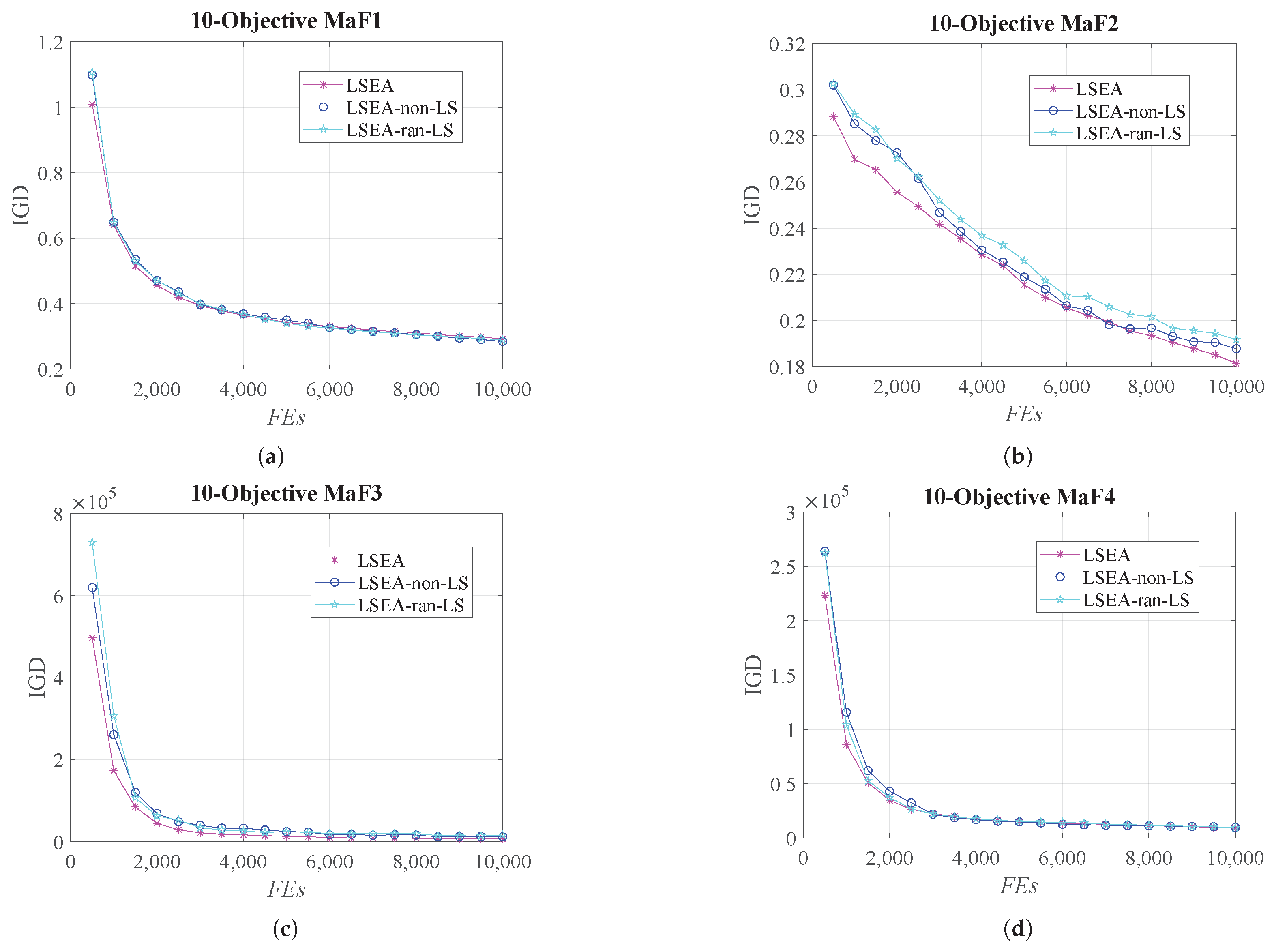
To distinguish the performance improvement of the local search mechanism, we constructed two variants of the proposed LSEA, denoted as LSEA-non-LS and LSEA-ran-LS. LSEA-non-LS was constructed by removing the local search mechanism from the LSEA. Unlike the LSEA, which selects a solution with better diversity and relatively poor convergence for local searches, its variant LSEA-ran-LS treats all solutions in the archive equally and selects one randomly. In the context of four test instances, i.e., 10-objective MaF1, MaF2, MaF3, and MaF4, this section compares the changes of the IGD values of LSEA, LSEA-non-LS, and LSEA-ran-LS during their evolution, as shown in Figure 5.
It can be observed in Figure 5 that the IGD values of the LSEA decrease faster than those of its two variants, especially in the early stage of the evolutionary search. This phenomenon demonstrates that the proposed local search mechanism proposed in this paper can effectively accelerate the populations toward the Pareto-optimal fronts. In addition, in the test instance 10-objective MaF2, the IGD values obtained by the LSEA were always lower than those of its two variants. This illustrates that the proposed local search mechanism can explore solutions with better convergence and diversity. By comparing LSEA-non-LS and LSEA-ran-LS, we found that the IGD value of the LSEA-ran-LS was smaller than that of LSEA-non-LS in most cases. This further demonstrates the performance improvement of the local search mechanism. The comparison results between LSEA and LSEA-ran-LS demonstrate that selecting solutions for local search according to the sum of their diversity and convergence is also beneficial to performance improvement.
4. Conclusions and Future Directions
This paper suggests adding an external archive for EMOA/Ds using weight-vector adjustment to give full play to their advantages, and we presented a selection mechanism without weight vectors to progressively improve both the convergence and diversity of the archive. Moreover, the proposed algorithm performed local searches on solutions with good diversity but relatively poor convergence to further strengthen convergence and diversity. In the proposed LSEA, once a new solution is reproduced, it will be associated with a solution with the minimum distance. Only the new solution has better convergence and diversity; it will replace the associated solution, progressively enlarging the diversity and convergence of the archive to well approximate irregular Pareto-optimal fronts. To examine the effectiveness of the proposed mechanism, it was compared with five baselines on 36 test instances with various Pareto-optimal front shapes, such as disconnected, degenerate, inverted, and strongly convex/concave. Numerical comparison results corroborate the superior performance of the LSEA in tackling MaOPs with irregular Pareto-optimal fronts: it significantly outperformed all the five baselines on 22 test instances concerning the metric HV.
Although LSEA possesses competitive advantages in solving MaOPs with various Pareto-optimal fronts, it still has two shortcomings. On the one hand, the validation of the LSEA was based on extensive numerical experiments, lacking rigorous theoretical proof. On the other hand, the LSEA has no significant advantages in tackling MaOPs with badly-scaled Pareto-optimal fronts, such as test instances derived from MaF4 and MaF5. Thus, in future work, we will extend the LSEA to handle MaOPs with a broader range of Pareto-optimal front shapes and research the theoretical basis of multi-objective evolutionary optimization.
Author Contributions
Conceptualization, L.X. and J.L.; methodology, J.L.; software, L.X. and R.W.; validation, L.X., R.W., J.C., and J.L.; formal analysis, R.W.; investigation, R.W.; resources, J.C.; data curation, J.C.; writing—original draft preparation, L.X.; writing—review and editing, R.W., J.C., and J.L.; visualization, J.C.; supervision, J.L.; project administration, J.L.; funding acquisition, J.L. All authors have read and agreed to the published version of the manuscript.
Funding
This research work is supported by the National Natural Science Foundation of China (61773120), the Special Projects in Key Fields of Universities in Guangdong (2021ZDZX1019), and the Hunan Provincial Innovation Foundation For Postgraduates (CX20200585).
Institutional Review Board Statement
Not applicable.
Informed Consent Statement
Not applicable.
Data Availability Statement
All data used during the study appear in the submitted article.
Conflicts of Interest
The authors declare no conflict of interest.
References
- Pham, T.P.; Fahringer, T. Evolutionary multi-objective workflow scheduling for volatile resources in the cloud. IEEE Trans. Cloud Comput. 2022, 10, 1780–1791. [Google Scholar] [CrossRef]
- Chen, H.; Zhu, X.; Liu, G.; Pedrycz, W. Uncertainty-aware online scheduling for real-time workflows in cloud service environment. IEEE Trans. Serv. Comput. 2021, 14, 1167–1178. [Google Scholar] [CrossRef]
- Li, H.; Wang, D.; Zhou, M.; Fan, Y.; Xia, Y. Multi-swarm co-evolution based hybrid intelligent optimization for bi-objective multi-workflow scheduling in the cloud. IEEE Trans. Parallel Distrib. Syst. 2022, 33, 2183–2197. [Google Scholar] [CrossRef]
- Chen, H.; Huang, H.; Zuo, X.; Zhao, X. Robustness enhancement of neural networks via architecture search with multi-objective evolutionary optimization. Mathematics 2022, 10, 2724. [Google Scholar] [CrossRef]
- Wang, Y.; Li, K.; Wang, G.G. Combining key-points-based transfer learning and hybrid prediction strategies for dynamic multi-objective optimization. Mathematics 2022, 10, 2117. [Google Scholar] [CrossRef]
- Yu, G.; Ma, L.; Jin, Y.; Du, W.; Liu, Q.; Zhang, H. A survey on knee-oriented multi-objective evolutionary optimization. IEEE Trans. Evol. Comput. 2023; in press. [Google Scholar]
- Stewart, R.H.; Palmer, T.S.; DuPont, B. A survey of multi-objective optimization methods and their applications for nuclear scientists and engineers. Prog. Nucl. Energy 2021, 138, 103830. [Google Scholar] [CrossRef]
- Falcón-Cardona, J.G.; Coello, C.A.C. Indicator-based multi-objective evolutionary algorithms: A comprehensive survey. ACM Comput. Surv. 2020, 53, 1–35. [Google Scholar] [CrossRef] [Green Version]
- Deb, K.; Pratap, A.; Agarwal, S.; Meyarivan, T. A fast and elitist multiobjective genetic algorithm: NSGA-II. IEEE Trans. Evol. Comput. 2002, 6, 182–197. [Google Scholar] [CrossRef] [Green Version]
- He, Z.; Yen, G.G.; Zhang, J. Fuzzy-based Pareto optimality for many-objective evolutionary algorithms. IEEE Trans. Evol. Comput. 2013, 18, 269–285. [Google Scholar] [CrossRef]
- Jiang, S.; Yang, S. A strength Pareto evolutionary algorithm based on reference direction for multiobjective and many-objective optimization. IEEE Trans. Evol. Comput. 2017, 21, 329–346. [Google Scholar] [CrossRef]
- Zitzler, E.; Thiele, L.; Laumanns, M.; Fonseca, C.M.; Da Fonseca, V.G. Performance assessment of multiobjective optimizers: An analysis and review. IEEE Trans. Evol. Comput. 2003, 7, 117–132. [Google Scholar] [CrossRef] [Green Version]
- Sun, Y.; Yen, G.G.; Yi, Z. IGD indicator-based evolutionary algorithm for many-objective optimization problems. IEEE Trans. Evol. Comput. 2018, 23, 173–187. [Google Scholar] [CrossRef] [Green Version]
- Zhang, Q.; Li, H. MOEA/D: A multiobjective evolutionary algorithm based on decomposition. IEEE Trans. Evol. Comput. 2007, 11, 712–731. [Google Scholar] [CrossRef]
- Trivedi, A.; Srinivasan, D.; Sanyal, K.; Ghosh, A. A survey of multiobjective evolutionary algorithms based on decomposition. IEEE Trans. Evol. Comput. 2017, 21, 440–462. [Google Scholar] [CrossRef]
- Das, I.; Dennis, J.E. Normal-boundary intersection: A new method for generating the Pareto surface in nonlinear multicriteria optimization problems. SIAM J. Optim. 1998, 8, 631–657. [Google Scholar] [CrossRef] [Green Version]
- Hua, Y.; Liu, Q.; Hao, K.; Jin, Y. A survey of evolutionary algorithms for multi-objective optimization problems with irregular Pareto fronts. IEEE/CAA J. Autom. Sin. 2021, 8, 303–318. [Google Scholar] [CrossRef]
- Liu, Q.; Jin, Y.; Heiderich, M.; Rodemann, T. Surrogate-assisted evolutionary optimization of expensive many-objective irregular problems. Knowl.-Based Syst. 2022, 240, 108197. [Google Scholar] [CrossRef]
- Tian, Y.; He, C.; Cheng, R.; Zhang, X. A multistage evolutionary algorithm for better diversity preservation in multiobjective optimization. IEEE Trans. Syst. Man, Cybern. Syst. 2021, 51, 5880–5894. [Google Scholar] [CrossRef]
- Cheng, R.; Jin, Y.; Olhofer, M.; Sendhoff, B. A reference vector guided evolutionary algorithm for many-objective optimization. IEEE Trans. Evol. Comput. 2016, 20, 773–791. [Google Scholar] [CrossRef] [Green Version]
- Kinoshita, T.; Masuyama, N.; Liu, Y.; Ishibuchi, H. Reference vector adaptation and mating selection strategy via adaptive resonance theory-based clustering for many-objective optimization. arXiv 2022, arXiv:2204.10756. [Google Scholar]
- Chen, H.; Cheng, R.; Pedrycz, W.; Jin, Y. Solving many-objective optimization problems via multistage evolutionary search. IEEE Trans. Syst. Man, Cybern. Syst. 2021, 51, 3552–3564. [Google Scholar] [CrossRef]
- Feng, W.; Gong, D.; Yu, Z. Multi-objective evolutionary optimization based on online perceiving Pareto front characteristics. Inf. Sci. 2021, 581, 912–931. [Google Scholar] [CrossRef]
- Ma, X.; Yu, Y.; Li, X.; Qi, Y.; Zhu, Z. A survey of weight vector adjustment methods for decomposition-based multiobjective evolutionary algorithms. IEEE Trans. Evol. Comput. 2020, 24, 634–649. [Google Scholar] [CrossRef]
- Li, M.; Yao, X. What weights work for you? Adapting weights for any Pareto front shape in decomposition-based evolutionary multiobjective optimisation. Evol. Comput. 2020, 28, 227–253. [Google Scholar] [CrossRef] [Green Version]
- Liu, Q.; Jin, Y.; Heiderich, M.; Rodemann, T. Coordinated Adaptation of Reference Vectors and Scalarizing Functions in Evolutionary Many-Objective Optimization. IEEE Trans. Syst. Man, Cybern. Syst. 2023; in press. [Google Scholar]
- Zhao, H.; Zhang, C. An online-learning-based evolutionary many-objective algorithm. Inf. Sci. 2020, 509, 1–21. [Google Scholar] [CrossRef]
- Zheng, W.; Sun, J. Two-stage hybrid learning-based multi-objective evolutionary algorithm based on objective space decomposition. Inf. Sci. 2022, 610, 1163–1186. [Google Scholar] [CrossRef]
- Gu, F.; Cheung, Y.M. Self-organizing map-based weight design for decomposition-based many-objective evolutionary algorithm. IEEE Trans. Evol. Comput. 2018, 22, 211–225. [Google Scholar] [CrossRef]
- Liu, Y.; Ishibuchi, H.; Masuyama, N.; Nojima, Y. Adapting reference vectors and scalarizing functions by growing neural gas to handle irregular Pareto fronts. IEEE Trans. Evol. Comput. 2020, 24, 439–453. [Google Scholar] [CrossRef]
- Liu, Q.; Jin, Y.; Heiderich, M.; Rodemann, T.; Yu, G. An adaptive reference vector-guided evolutionary algorithm using growing neural gas for many-objective optimization of irregular problems. IEEE Trans. Cybern. 2022, 52, 2698–2711. [Google Scholar] [CrossRef]
- Jain, H.; Deb, K. An evolutionary many-objective optimization algorithm using reference-point based nondominated sorting approach, part II: Handling constraints and extending to an adaptive approach. IEEE Trans. Evol. Comput. 2014, 18, 602–622. [Google Scholar] [CrossRef]
- Elarbi, M.; Bechikh, S.; Coello, C.A.C.; Makhlouf, M.; Said, L.B. Approximating complex Pareto fronts with predefined normal-boundary intersection directions. IEEE Trans. Evol. Comput. 2020, 24, 809–823. [Google Scholar] [CrossRef]
- Das, S.; Mullick, S.S.; Suganthan, P.N. Recent advances in differential evolution–an updated survey. Swarm Evol. Comput. 2016, 27, 1–30. [Google Scholar] [CrossRef]
- Liu, Q.; Cui, C.; Fan, Q. Self-adaptive constrained multi-objective differential evolution algorithm based on the state–action–reward–state–action method. Mathematics 2022, 10, 813. [Google Scholar] [CrossRef]
- Abed-alguni, B.H.; Alawad, N.A.; Barhoush, M.; Hammad, R. Exploratory cuckoo search for solving single-objective optimization problems. Soft Comput. 2021, 25, 10167–10180. [Google Scholar] [CrossRef]
- Alkhateeb, F.; Abed-alguni, B.H.; Al-rousan, M.H. Discrete hybrid cuckoo search and simulated annealing algorithm for solving the job shop scheduling problem. J. Supercomput. 2022, 78, 4799–4826. [Google Scholar] [CrossRef]
- Wang, G.; Guo, L.; Wang, H.; Duan, H.; Liu, L.; Li, J. Incorporating mutation scheme into krill herd algorithm for global numerical optimization. Neural Comput. Appl. 2014, 24, 853–871. [Google Scholar] [CrossRef]
- Meghwani, S.S.; Thakur, M. Adaptively weighted decomposition based multi-objective evolutionary algorithm. Appl. Intell. 2020, 51, 1–23. [Google Scholar] [CrossRef]
- Li, K. Decomposition Multi-Objective Evolutionary Optimization: From State-of-the-Art to Future Opportunities. arXiv 2021, arXiv:2108.09588. [Google Scholar]
- Yang, M.; Li, C.; Cai, Z.; Guan, J. Differential evolution with auto-enhanced population diversity. IEEE Trans. Cybern. 2014, 45, 302–315. [Google Scholar] [CrossRef]
- Tian, Y.; Cheng, R.; Zhang, X.; Li, M.; Jin, Y. Diversity assessment of multi-objective evolutionary algorithms: Performance metric and benchmark problems. IEEE Comput. Intell. Mag. 2019, 14, 61–74. [Google Scholar] [CrossRef]
- Li, L.; Yen, G.G.; Sahoo, A.; Chang, L.; Gu, T. On the estimation of Pareto front and dimensional similarity in many-objective evolutionary algorithm. Inf. Sci. 2021, 563, 375–400. [Google Scholar] [CrossRef]
- Takagi, T.; Takadama, K.; Sato, H. A distribution control of weight vector set for multi-objective evolutionary algorithms. In Proceedings of the International Conference on Bio-inspired Information and Communication, Pittsburgh, PA, USA, 13–14 March 2019; pp. 70–80. [Google Scholar]
- Deb, K.; Jain, H. An evolutionary many-objective optimization algorithm using reference-point-based nondominated sorting approach, part I: Solving problems with box constraints. IEEE Trans. Evol. Comput. 2014, 18, 577–601. [Google Scholar] [CrossRef]
- Wang, R.; Zhang, Q.; Zhang, T. Decomposition-based algorithms using Pareto adaptive scalarizing methods. IEEE Trans. Evol. Comput. 2016, 20, 821–837. [Google Scholar] [CrossRef]
- Tian, Y.; Cheng, R.; Zhang, X.; Jin, Y. PlatEMO: A MATLAB Platform for Evolutionary Multi-Objective Optimization. IEEE Comput. Intell. Mag. 2017, 12, 73–87. [Google Scholar] [CrossRef] [Green Version]
- Cheng, R.; Li, M.; Tian, Y.; Zhang, X.; Yang, S.; Jin, Y.; Yao, X. A benchmark test suite for evolutionary many-objective optimization. Complex Intell. Syst. 2017, 3, 67–81. [Google Scholar] [CrossRef]
- Hua, Y.; Jin, Y.; Hao, K. A clustering-based adaptive evolutionary algorithm for multiobjective optimization with irregular Pareto fronts. IEEE Trans. Cybern. 2019, 49, 2758–2770. [Google Scholar] [CrossRef]
- Chen, H.; Cheng, R.; Wen, J.; Li, H.; Weng, J. Solving large-scale many-objective optimization problems by covariance matrix adaptation evolution strategy with scalable small subpopulations. Inf. Sci. 2020, 509, 457–469. [Google Scholar] [CrossRef]
- Zitzler, E.; Thiele, L. Multiobjective evolutionary algorithms: A comparative case study and the strength Pareto approach. IEEE Trans. Evol. Comput. 1999, 3, 257–271. [Google Scholar] [CrossRef] [Green Version]
- Bosman, P.A.; Thierens, D. The balance between proximity and diversity in multiobjective evolutionary algorithms. IEEE Trans. Evol. Comput. 2003, 7, 174–188. [Google Scholar] [CrossRef] [Green Version]
- Li, M.; Zhen, L.; Yao, X. How to read many-objective solution sets in parallel coordinates. IEEE Comput. Intell. Mag. 2017, 12, 88–100. [Google Scholar] [CrossRef]
Figure 1.
An illustrative example of the local search. (a) select a solution with good diversity, (b) explore the sparse region by the local search.
Figure 1.
An illustrative example of the local search. (a) select a solution with good diversity, (b) explore the sparse region by the local search.

Figure 2.
Distributions of populations obtained by the six algorithms in the 10-objective MaF1. (a) output population of MaOEA-IGD, (b) output population of DEA-GNG, (c) output population of MaOEA-IGD, (d) output population of NSGA-III, (e) output population of MOEA/D-PaS, (f) output population of LSEA.

Figure 3.
Distributions of populations obtained by the six algorithms on 10-objective MaF6. (a) output population of MaOEA-IGD, (b) output population of DEA-GNG, (c) output population of MaOEA-IGD, (d) output population of NSGA-III, (e) output population of MOEA/D-PaS, (f) output population of LSEA.

Figure 4.
Distributions of populations in decision space of the six algorithms on 10-objective MaF8. (a) output population of MaOEA-IGD, (b) output population of DEA-GNG, (c) output population of MaOEA-IGD, (d) output population of NSGA-III, (e) output population of MOEA/D-PaS, (f) output population of LSEA.

Figure 5.
Changes in the IGD values of LSEA, LSEA-non-LS, and LSEA-ran-LS, where denotes the number of function evaluations. (a) on 10-objective MaF1, (b) on 10-objective MaF2, (c) on 10-objective MaF3, (d) on 10-objective MaF4.
Figure 5.
Changes in the IGD values of LSEA, LSEA-non-LS, and LSEA-ran-LS, where denotes the number of function evaluations. (a) on 10-objective MaF1, (b) on 10-objective MaF2, (c) on 10-objective MaF3, (d) on 10-objective MaF4.


Table 1.
HV values (average and standard deviation) obtained by the LSEA and the five baselines on MaF1–MaF9 with 5, 10, 13, and 15 objectives. Highest average HV value on each test instance is highlighted with a gray background.
Table 1.
HV values (average and standard deviation) obtained by the LSEA and the five baselines on MaF1–MaF9 with 5, 10, 13, and 15 objectives. Highest average HV value on each test instance is highlighted with a gray background.
| MOPs | m | MOEA/D-CWV | DEA-GNG | MaOEA/IGD | NSGA-III | MOEA/D-PaS | LSEA |
|---|---|---|---|---|---|---|---|
| MaF1 | 5 | () − | () − | () − | () − | () − | () |
| 10 | () − | () − | () − | () − | () − | () | |
| 13 | () − | () − | () − | () − | () − | () | |
| 15 | () − | () − | () − | () − | () − | () | |
| MaF2 | 5 | () − | () − | () − | () − | () − | () |
| 10 | () − | () − | () − | () + | () − | () | |
| 13 | () − | () − | () − | () + | () − | () | |
| 15 | () − | () − | () − | () + | () − | () | |
| MaF3 | 5 | () − | () − | () − | () + | () ≈ | () |
| 10 | () − | () − | () − | () − | () − | () | |
| 13 | () − | () − | () − | () − | () − | () | |
| 15 | () − | () − | () − | () − | () − | () | |
| MaF4 | 5 | () − | () ≈ | () − | () − | () − | () |
| 10 | () − | () + | () − | () − | () − | () | |
| 13 | () − | () ≈ | () − | () + | () − | () | |
| 15 | () − | () ≈ | () − | () + | () − | () | |
| MaF5 | 5 | () − | () + | () − | () + | () + | () |
| 10 | () − | () + | () − | () + | () + | () | |
| 13 | () − | () + | () − | () + | () + | () | |
| 15 | () − | () + | () − | () + | () + | () | |
| MaF6 | 5 | () − | () ≈ | () − | () − | () − | () |
| 10 | () − | () − | () − | () − | () − | () | |
| 13 | () − | () − | () − | () − | () − | () | |
| 15 | () − | () − | () − | () − | () − | () | |
| MaF7 | 5 | () − | () − | () − | () − | () − | () |
| 10 | () − | () ≈ | () − | () + | () − | () | |
| 13 | () − | () + | () − | () ≈ | () − | () | |
| 15 | () ≈ | () ≈ | () ≈ | () ≈ | () ≈ | () | |
| MaF8 | 5 | () − | () − | () − | () − | () − | () |
| 10 | () − | () − | () − | () − | () − | () | |
| 13 | () − | () − | () − | () − | () − | () | |
| 15 | () − | () − | () − | () − | () − | () | |
| MaF9 | 5 | () − | () − | () − | () − | () − | () |
| 10 | () − | () − | () − | () − | () − | () | |
| 13 | () − | () − | () − | () − | () − | () | |
| 15 | () − | () − | () − | () − | () − | () | |
| −/+/≈ | 35/0/1 | 25/6/5 | 35/0/1 | 23/11/2 | 30/4/2 |
Table 2.
IGD values (average and standard deviation) obtained by the LSEA and the five baselines on the MaF1-MaF9 with 5, 10, 13, and 15 objectives. The lowest average IGD value on each test instance is highlighted with a gray background.
Table 2.
IGD values (average and standard deviation) obtained by the LSEA and the five baselines on the MaF1-MaF9 with 5, 10, 13, and 15 objectives. The lowest average IGD value on each test instance is highlighted with a gray background.
| MOPs | m | MOEA/D-CWV | DEA-GNG | MaOEA/IGD | NSGA-III | MOEA/D-PaS | LSEA |
|---|---|---|---|---|---|---|---|
| MaF1 | 5 | () − | () + | () − | () − | () − | () |
| 10 | () − | () − | () − | () − | () − | () | |
| 13 | () − | () − | () − | () + | () − | () | |
| 15 | () − | () − | () − | () − | () − | () | |
| MaF2 | 5 | () − | () ≈ | () − | () − | () − | () |
| 10 | () − | () − | () − | () − | () − | () | |
| 13 | () − | () − | () − | () + | () − | () | |
| 15 | () − | () − | () − | () + | () − | () | |
| MaF3 | 5 | () − | () ≈ | () − | () + | () ≈ | () |
| 10 | () − | () − | () − | () − | () − | () | |
| 13 | () − | () − | () − | () − | () − | () | |
| 15 | () − | () − | () − | () − | () − | () | |
| MaF4 | 5 | () − | () − | () − | () − | () − | () |
| 10 | () − | () ≈ | () − | () − | () − | () | |
| 13 | () − | () + | () − | () ≈ | () − | () | |
| 15 | () − | () + | () − | () + | () − | () | |
| MaF5 | 5 | () − | () + | () + | () + | () + | () |
| 10 | () − | () + | () − | () + | () + | () | |
| 13 | () − | () + | () − | () + | () − | () | |
| 15 | () − | () + | () − | () + | () ≈ | () | |
| MaF6 | 5 | () − | () − | () − | () − | () − | () |
| 10 | () − | () − | () − | () − | () − | () | |
| 13 | () − | () − | () − | () − | 2.4674 × 10+2 () − | () | |
| 15 | () − | () − | () − | () − | () − | () | |
| MaF7 | 5 | () − | () + | () − | () − | () − | () |
| 10 | () − | () + | () − | () − | () − | () | |
| 13 | () − | () − | () − | () − | () − | () | |
| 15 | () ≈ | () ≈ | () ≈ | () ≈ | () ≈ | () | |
| MaF8 | 5 | () − | () − | () − | () − | () − | () |
| 10 | () − | () − | () − | () − | (1.46 × 10+1) − | () | |
| 13 | () − | () − | () − | () − | () − | () | |
| 15 | () − | () − | () − | () − | () − | () | |
| MaF9 | 5 | () − | () − | () − | () − | () − | () |
| 10 | () − | () − | () − | () − | () − | () | |
| 13 | () − | () − | () − | () − | () − | () | |
| 15 | () − | () − | () − | () − | () − | () | |
| −/+/≈ | 35/0/1 | 23/9/4 | 34/1/1 | 25/9/2 | 32/2/2 |
Disclaimer/Publisher’s Note: The statements, opinions and data contained in all publications are solely those of the individual author(s) and contributor(s) and not of MDPI and/or the editor(s). MDPI and/or the editor(s) disclaim responsibility for any injury to people or property resulting from any ideas, methods, instructions or products referred to in the content. |
© 2022 by the authors. Licensee MDPI, Basel, Switzerland. This article is an open access article distributed under the terms and conditions of the Creative Commons Attribution (CC BY) license (https://creativecommons.org/licenses/by/4.0/).
Share and Cite
MDPI and ACS Style
Xing, L.; Wu, R.; Chen, J.; Li, J. Handling Irregular Many-Objective Optimization Problems via Performing Local Searches on External Archives. Mathematics 2023, 11, 10. https://0-doi-org.brum.beds.ac.uk/10.3390/math11010010
AMA Style
Xing L, Wu R, Chen J, Li J. Handling Irregular Many-Objective Optimization Problems via Performing Local Searches on External Archives. Mathematics. 2023; 11(1):10. https://0-doi-org.brum.beds.ac.uk/10.3390/math11010010
Chicago/Turabian StyleXing, Lining, Rui Wu, Jiaxing Chen, and Jun Li. 2023. "Handling Irregular Many-Objective Optimization Problems via Performing Local Searches on External Archives" Mathematics 11, no. 1: 10. https://0-doi-org.brum.beds.ac.uk/10.3390/math11010010
Note that from the first issue of 2016, this journal uses article numbers instead of page numbers. See further details here.