
Active Debris Removal Mission Planning Method Based on Machine Learning

1
College of System Engineering, National University of Defense Technology, Changsha 410073, China
2
College of Aerospace Science and Engineering, National University of Defense Technology, Changsha 410073, China
*
Author to whom correspondence should be addressed.
Mathematics 2023, 11(6), 1419; https://0-doi-org.brum.beds.ac.uk/10.3390/math11061419
Submission received: 22 February 2023
/
Revised: 11 March 2023
/
Accepted: 13 March 2023
/
Published: 15 March 2023
(This article belongs to the Special Issue Evolutionary Computation 2022)
Abstract
:To prevent the proliferation of space debris and stabilize the space environment, active debris removal (ADR) has increasingly gained public concern. Considering the complexity of space operations and the viability of ADR missions, it would be necessary to schedule the ADR process in order to remove as much debris as possible. This paper presents an active debris removal mission planning problem, devoted to generate an optimal debris removal plan to guide the mission process. According to the problem characteristics, a two-layer time-dependent traveling salesman problem(TSP) mathematical model is established, involving the debris removal sequence planning and the transfer trajectory planning. Subsequently, two main novel methods based on machine learning are proposed for the ADR mission planning problem, including a deep neural networks(DNN)-based estimation method for approximating the optimal velocity increments of perturbed multiple-impulse rendezvous and an reinforcement learning(RL)-based method for optimizing the sequence of debris removal and rendezvous time. Experimental results of different simulation scenarios have verified the effectiveness and superiority of the proposed method, indicating the good performance for solving the active debris removal mission planning problem.
Keywords:
active space debris removal; mission planning; time-dependent TSP; transfer estimation; sequence planning; deep neural networks; pointer network; reinforcement learningMSC:
68M20; 90B351. Introduction
1.1. Background
In the past 60 years, mankind has been actively exploring and developing near-Earth space through rockets, satellites, and other kinds of spacecraft. A by-product of this activity is space debris, which is structural fragments, the upper stages of rockets, or even the abandoned satellite itself after completing its mission [1]. The debris can stay in orbit for decades or even hundreds of years, posing a serious threat to both functioning and newly launched satellites and spacecraft. Kessler and Cour-Palais [2] put forward the “Kessler syndrome”, which attracted widespread attention. The theory pointed out a dramatic situation of space debris, when the collision of two large objects of space debris causes an avalanche-like cascade of mutual collisions, ultimately leading to the formation of a cloud of debris around the Earth [3]. Research shows that at least five large space debris need to be removed every year to stabilize the space environment [4,5].
Realizing the huge danger posed by space debris, scholars have proposed the concept of Active Space Debris Removal (ADR). Various approaches have been developed to remove space debris: contact approaches, such as through robotic arm [6,7], nets [8,9], tethered space robots [10,11], and harpoon [12,13,14], and contactless approaches, such as through ion beam assisted transportation [15,16], electrostatic transportation [17,18], laser transportation [19,20], gravity transportation [21,22], and electromagnetic detumbling [23,24]. However, due to the complexity of space mission operations and the scarcity of on-orbit servicing spacecraft resources, the implementation of the active space debris removal mission requires continuous and systematic planning measures.
Active space debris removal mission planning problem is a complex optimization problem, which is used to determine the sequence of debris removal, rendezvous time, and transfer trajectory between two adjacent debris removal processes.
The combinatorial optimization characteristics of the problem are similar to those of the traveling salesman problem (TSP) [25] to a degree, but compared with it, ADR mission planning problem shows greater complexity and difficulty in solving. This can be summarized in two aspects: first, the calculation of the optimal transfer velocity increment between two debris is much more complicated than the calculation of the Euclidean distance between two cities with a fixed location, and it is particularly time-consuming; second, because space debris runs in different orbits and its spatial location changes with time, ADR mission planning problem has a larger search space than the classic TSP problem of the same scale. Thus, effective and efficient planning methods are of crucial significance for the completion of the ADR missions.
1.2. Literature Review
At present, the methods for solving active space debris removal mission planning problem can be divided into three main categories: explicit enumeration methods, implicit enumeration methods, and meta-heuristic methods [26].
- (1)
- Explicit enumeration methods
The explicit enumeration methods are committed to finding the exact global optimal solution by enumerating all possible combinations. This method is only applicable when the search space is very small. Zuiani and Vasile [27] presented a simplified ADR mission planning scenario of five space debris under the preliminary design of low-thrust, many-revolution transfers. According to different propulsion systems, Braun et al. [28] proposed four space debris removal modes and the best removal sequence of four to six debris is obtained through the brute-force approach. However, when the number of debris is larger than 10, the considerable calculation time of enumerating all feasible combinations is unacceptable.
- (2)
- Implicit enumeration methods
Implicit enumeration methods are committed to explore the optimization process by finding those sequences with high probabilities of becoming the optimal solution and pruning other sequences [29]. The tree search algorithm can be regarded as a typical implicit enumeration method, and the tree nodes represent the space debris involved in orbital transfers. The pruning strategy is crucial to the tree search algorithm, because excessive pruning may lose the optimal solution and inadequate pruning will increase the computational burden [26]. Li et al. [30] proposed a beam search algorithm with the pruning strategy, in which only the first beam width’s number of nodes was expanded for the next level, and the others were abandoned. Branch and bound is another effective pruning strategy. Olympio and Frouvelle [31] studied a space debris removal mission in solar synchronous orbit with perturbation considered, and designed the branch and prune algorithm with a pruning strategy to accelerate the removal sequence search process. Barea et al. [32] divided the ADR mission planning problem into two layers: the upper layer constructed a linear integer model, and the lower layer constructed a nonlinear mixed integer model and applied the branch and bound algorithm to search the best removal sequence. Cerf [26] used the branch and bound algorithm to optimize the debris removal sequence and transfer trajectory to obtain a optimal debris removal scheme with the minimum total propellant consumption. Further considering the mission completion time, Madakat et al. [33] modeled the problem as a multi-objective time-dependent traveling salesman problem (TDTSP) with the objective of minimizing the total mission time and total propellant consumption, and adopted the branch and bound algorithm to find the optimal solution for low-Earth-orbit(LEO) space debris removal. Olive et al. [34] further built the TOPAS platform (Tool for Optimal Planning of ADR Sequence) based on the branch and bound algorithm, which was applicable to complex ADR scenarios with up to 10 space debris.
However, in most of the cases mentioned above, still only small amount of space debris removal is scheduled. When it comes to cases of large scale, implicit enumeration methods may not be efficient and a suitable approach for ADR mission planning of a complicated characteristic of mixed integer programming is required.
- (3)
- Meta-heuristic methods
The meta-heuristic methods possess a great potential for finding the near-optimal solution within an acceptable time, and provide another idea for solving the ADR mission planning problem. In recent research, genetic algorithm (GA) [35], simulated annealing (SA) [36], Physarum Algorithm [37,38], particle swarm optimization (PSO) [39], and ant colony optimization (ACO) [40] have been applied to schedule debris removal missions.
Murakami and Hokamoto [41] proposed two transfer trajectory selection rules to simplify the transfer trajectory optimization problem, and used GA by encoding the removal sequence and the transfer time into the chromosome together. Liu et al. [42] was devoted to developing a preliminary plan for a multi-nanosatellite active debris removal platform (MnADRP) for LEO missions and a dynamic multi-objective TSP scheme was proposed in which three optimization objectives, i.e., the debris removal priority, the MnADRP orbital transfer energy, and the number of required nanosatellites were modeled, respectively. Chen et al. [43] proposed a GA-based three-stage removal strategy for space debris: the first stage to develop the mission scenario with multiple spacecraft including one main spacecraft and some following spacecraft for debris removal missions; the second stage to define the fuel, time, and the quantity of the following spacecraft as the constraints; and the third stage to establish the mathematical model taking the minimum fuel consumption as the optimal objective. Missel and Mortari [44] studied the Space Sweeper with Sling-Sat (4S) mission of debris removal and optimized the combinatory selecting of the debris interaction order, ejection velocities, and sequence timing by an evolutionary algorithm. Federici et al. [3] designed an effective coding and mutation operator, and applied SA to optimize the removal sequence and the rendezvous time of ADR missions, which could accomplish the removal mission planning for 20 space debris. Medioni et al. [45] performed optimization using SA and a tool to classify the targets in groups gathered by similarities of orbital elements, with the objective for each mission being not to exceed a total km/s, and for a mission time lower than 3 years, which was proposed for removal target selection. Carlo et al. [46] proposed TSP and VRP(Vehicle Routing Problem) modeling strategies, respectively, for LEO ADR missions and designed a bio-inspired incremental automatic planning and scheduling discrete optimization algorithm based on the Physarum algorithm. Oriented to the geostationary-orbit(GEO) debris removal mission planning problem, Jing et al. [47] studied three key sub-problems: mission allocation, sequence planning, and trajectory transfer planning, which were modeled by a hybrid optimal control model and solved by an improved multi-objective PSO. Mohammadi-Dehabadi et al. [48] designed a multi-objective PSO algorithm for minimizing the total propellant consumption and mission completion time and, through their experiments, it was shown that the initial orbital elements of the spacecraft had a great impact on the propellant consumption and time cost for ADR missions. Stuart et al. [49] used ACO to generate a preliminary debris removal sequence and to determine the number of spacecrafts required to clear a debris set, and re-planned the preliminary scheme by multi-agent coordination via auctions. Shen et al. [50] used ACO to optimize the sequence planning model for the dynamic ADR mission planning problem under perturbation, and successfully obtained the optimal removal sequence of 10 debris. Zhang et al. [51] proposed an improved ACO with the inner-outer operator, whose effectiveness to select the optimal removal targets from a large set of debris (up to 2000) was proved by their experiments. Li and Baoyin [52] combined the advantage of an evolutionary algorithm and population intelligence algorithm, took ACO as the framework and added the GA operator, and developed the evolutionary elitist club algorithm (EECA) to optimize the multi-debris removal mission. Zhu [53] designed the dynamic sequence planning ant colony optimization algorithm based on the framework of the ant colony system, introduced the concept of a pheromone tensor to characterize the dynamic transfer preference between debris targets, and proposed a step-by-step rendezvous sequence planning strategy based on the time discretization method. Unlike the methods described in refs. [52,53], which added the time dimension into the pheromone matrix of the ACO by discretizing and fitting time, Zhang et al. [29] directly put the timeline particles at a certain moment of the corresponding timeline, but not at a series of discrete time points and solved the time-dependent characteristics of the ADR mission planning problem through a new structure called the Timeline Club.
As can be seen from the above, the literature may fall into three main drawbacks. First, most of the ADR mission merely involved several debris and did not discuss the situation with large-scale debris. Second, in order to simplify the planning problem, some studies adopted a static and non-time-varying transfer trajectory model, which was far from the actual situation. Last but not the least, a hierarchical optimization strategy was often adopted to decompose the ADR mission planning problem where the debris removal sequence and transfer trajectory were optimized separately. Consequently, the final solution may not be optimal without a global optimization.
Therefore, this paper develops two novel methods to confront the deficiencies above, including a method for estimating the optimal velocity increments of perturbed multiple-impulse rendezvous for actual transfer trajectory planning and a method for optimizing the sequence of debris removal and transfer trajectory simultaneously.
1.3. Contributions
This paper is devoted to solve the high complexity of the combination optimization in the active debris removal mission planning problem and proposes an ADR planning method based on machine learning, which performs well. The main contributions of this paper are summarized as follows.
- (1)
- A two-layer time-dependent TSP mathematical model is proposed, which clarifies the structure and characteristics of the ADR mission planning problem. Based on this model, the solving method is designed subsequently;
- (2)
- A deep neural networks(DNN)-based estimation method for approximating the optimal velocity increments of perturbed multiple-impulse rendezvous is proposed, which overcomes the deficiency of time consumption for optimizing the velocity increments using conventional methods. Its accuracy is much higher than typical analytical approximation methods;
- (3)
- An reinforcement learning(RL)-based method for debris removal sequence planning is introduced for the first time. Unlike traditional intelligence optimization algorithms, the RL-based method can quickly generate solutions after training and learning, which is much more appropriate when it comes to large-scale debris removal situation.
The reminder of this paper is outlined as follows: Section 2 first defines the ADR mission planning problem and then transforms it into a special time-dependent TSP problem within several criteria and constraints. Based on that, it formally demonstrates a two-layer time-dependent TSP mathematical model to address the problem. Section 3 describes two main methods for solving the ADR mission planning problem, including a DNN-based estimation method for the optimal velocity increments of perturbed multiple-impulse rendezvous and an RL-based planning method for optimizing the sequence of debris removal. Section 4 first presents the design of two different test scenarios and then evaluates the performance of the proposed approach. In Section 5, the conclusions are given.
2. Mathematical Model
2.1. Problem Description
In this work, the problem is referred to as the active space debris removal mission planning problem, which is devoted to generate an optimal debris removal plan to guide the mission process.
The active space debris removal mission planning problem mainly involves the optimization of the removal sequence, rendezvous time, and transfer trajectory between two adjacent debris. According to the problem characteristics, the problem can be decomposed into two layers, as shown in Figure 1. The outer layer is the debris removal sequence planning, which optimizes the debris removal sequence and rendezvous time. The inner layer is the transfer trajectory planning, which optimizes the transfer time and transfer velocity increment. Note that, although the problem is decomposed into two layers in order to address it more clearly, the two layers are considered simultaneously by the following described solving methods.
The removal sequence is denoted by the removal order of the space debris targets. The removal order number is an integer variable while the rendezvous time, transfer time, and the transfer velocity increment are both real variables. It can be seen that this problem is a two-layer mixed integer optimization problem, and its difficulty lies in its nested optimization attribute and mixed integer variable characteristics.
Typically, adjusting the rendezvous time between spacecraft and debris with the removal sequence determined has a relatively small impact on the overall fulfillment of the mission. However, if the removal sequence is changed, the overall propulsion consumption may be greatly affected, or even exceed the maximum spacecraft loading capacity. Therefore, the debris removal sequence planning focuses more on the rendezvous order for spacecraft and debris, making it similar to the TSP problem to a certain degree. Variously, the classic TSP problem is a static target visiting sequence planning problem with a fixed city location, while the debris removal sequence planning is a time-dependent rendezvous sequence planning problem for moving targets, typically a time-dependent TSP problem (TD-TSP) [54], as shown in Figure 2. In the moving target rendezvous problem, the traveler can stay with the target for a period of time, or he can set out immediately for the next target.
Although we focus more on the debris removal sequence, it cannot be optimized regardless of the rendezvous time. Otherwise, only the static debris removal sequence is obtained, which has no practical significance. However, since the rendezvous time is a continuous real variable, it is impractical to search its optimization space entirely. Thus, a time discretization strategy is adopted. As shown in Figure 3, the rendezvous time between spacecraft and space debris is no longer a continuous value in the time interval, but only the time point represented by each discrete spot after discretization. Obviously, the search space of the time-dependent sequence planning problem has been greatly reduced, laying a foundation for the efficient solution of the problem.
As for the inner layer, i.e., the transfer trajectory planning, perturbed multiple-impulse transfer is involved. For the transfer trajectory planning problem where the rendezvous between two targets is caused by two impulses, if the initial and terminal conditions are given, the transfer velocity increment is a certain value, which can be directly solved by the Lambert algorithm. However, for the problem of perturbed multiple-impulse rendezvous, the transfer velocity increment is no longer a fixed value, and the optimal value needs to be obtained through optimization. The perturbation in this paper is referred to as the perturbation [30], which is caused by the Earth’s oblateness. perturbation will affect the right ascension of the ascending node (RAAN) of the orbit for both the spacecraft and debris and add the complexity of solving the inner problem.
2.2. A Two-Layer TD-TSP Mathematical Model
Based on the analysis above, the mathematical model of the active space debris removal mission planning problem is constructed as a two-layer TD-TSP model.
- (1)
- Decision variable
The main variables to be considered include the debris removal sequence, rendezvous time, and the relevant impulse parameters of spacecraft transfer. According to the two-layer attribute of the problem, the outer and inner decision variables can be designed, respectively.
The outer variable is defined in Equation (1).
where N represents the number of space debris, represents the removal order for debris i, represents the rendezvous time between the spacecraft and debris i, and represents the departure time of the spacecraft from debris i.
The inner design variables include two types, respectively representing the impulse time and impulse vector, and are defined in Equations (2) and (3).
where n is the number of the involved impulses. points to the three components of the vector.
- (2)
- Constraints
Similarly, the constraints will also be described in two layers.
(i) Outer constraints
Equation (4) indicates that the value of the debris removal sequence is a positive integer within , and the same debris cannot be removed repeatedly.
Equation (5) restricts that the rendezvous time between the spacecraft and the next debris must be later than the departure time from the previous debris.
Equation (6) means that the waiting time of the spacecraft should be longer than the minimum operating time, that is, the spacecraft needs to stay in the target orbit for a sufficient time to achieve debris removal operation.
(ii) Inner constraints
Equation (7) indicates that the impulses should be applied in sequence and the th impulse should be later than the ith impulse.
Equation (8) denotes the conditions to judge whether the spacecraft and debris rendezvous, where and are respectively the position and velocity vector of the spacecraft and debris, and and are the maximum allowable position and velocity error for rendezvous.
- (3)
- Optimization objective
The active space debris removal mission planning problem aims to complete the space debris removal mission with the goal of maximizing the utilization efficiency of spacecraft resource and minimizing the impulse propellant consumption subject to constraints.
Equation (9) addresses the sequence optimization objective for the outer layer. is the optimal impulse velocity increment for the transfer between debris i to debris .
Equation (10) addresses the transfer trajectory optimization objective for the inner layer, which is to minimize the impulse velocity increment for a certain transfer, related to the impulse vector. represents the jth impulse velocity increment from debris i to debris .
Therefore, the overall optimization objective for the active space debris removal mission planning problem can be expressed as Equation (11).
3. Methods
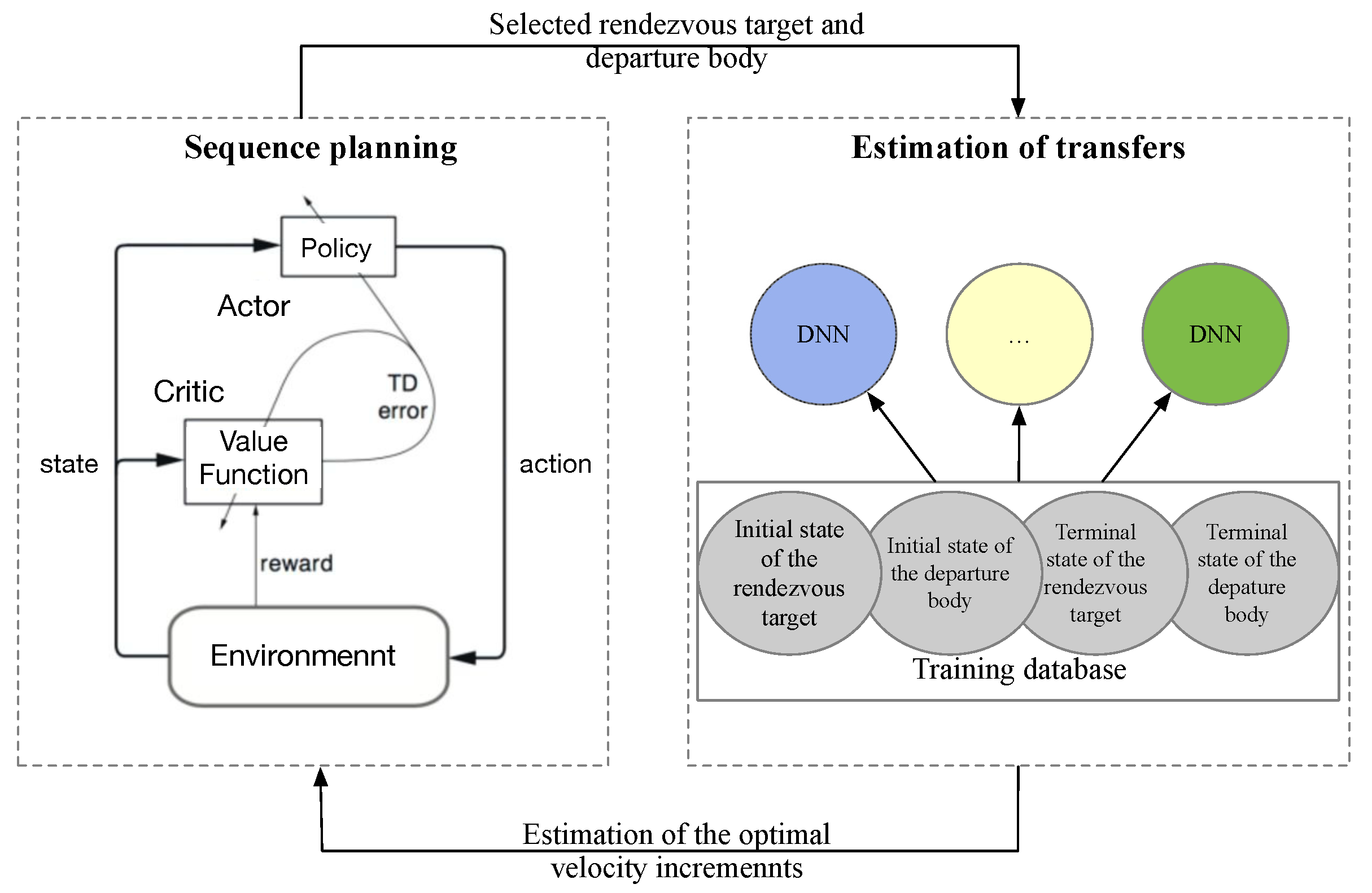
Figure 4 illustrates the whole framework of the active debris removal mission planning method based on machine learning, which is composed of two main connected segments, namely the estimation of transfers and sequence planning. Accordingly, the two main parts of the method are addressed as follows.
3.1. A DNN-Based Estimation Method for Approximating the Optimal Velocity Increments of Perturbed Multiple-Impulse Rendezvous
The debris removal sequence planning needs to quickly obtain the transfer cost (velocity increment) between any two targets in a given initial and terminal state in order to evaluate the profit of the removal sequence plan. However, unlike the rendezvous caused by two impulses, the transfer cost for perturbed multiple-impulse rendezvous is no longer a fixed value and needs to be optimized. This is usually a time-consuming process. If it is nested in the sequence planning, optimizing the removal order and transfer trajectory simultaneously, the calculation time will be unacceptable. Therefore, to solve the ADR mission planning problem, a method that can quickly and accurately estimate the optimal velocity increments of perturbed multiple-impulse rendezvous is demanded.
Previously, researchers basically used analytical methods to roughly estimate the optimal velocity increment. This kind of method is fast, but its estimation accuracy is not high under the circumstances of perturbed multiple-impulse rendezvous. Large estimation errors will directly affect sequence optimization in the outer layer. Thus, a method for estimating the optimal velocity increments of perturbed multiple-impulse rendezvous based on deep neural networks (DNN) is proposed.
First of all, the perturbed multiple-impulse rendezvous can be divided into three types according to the difference variation trend of the right ascension of the ascending node () between the departure body and the rendezvous target. They are “-closing rendezvous”, “-intersecting rendezvous”, and “-separating rendezvous” [53], as illustrated in Figure 5. The estimation of optimal velocity increments of the three types is implemented separately. The whole solving framework of the estimation method for perturbed multiple-impulse rendezvous is depicted in Figure 6.
- Step 1: Build a training database.
The database is required to cover three types of the perturbed multiple-impulse rendezvous cases with different parameters and conditions for training. A two-step approach including an improved differential evolution (DE) [55] algorithm and a sequential quadratic programming (SQP) algorithm [56] is applied as the optimizer to generate the rendezvous solution for each case. More detailed information on the parameters and implementations for building the database is presented in Section 4.1.
- Step 2: Train the deep neural network.
Three deep neural networks are demanded for training the three types of the perturbed multiple-impulse rendezvous.
A deep neural network is a complex nonlinear system composed of a large number of interconnected neurons (nodes) [57]. Each node obtains one or more inputs from other nodes, and generates an output through an activation function over the weighted sum of these inputs. Neural networks have many different network structures, and most of them contain three types of layers: input layer, hidden layer, and output layer. For general regression problems, the fully connected multi-layer perceptron (MLP) is usually a more suitable network model [58]. A well-trained MLP with a moderate network size can approximate any complex nonlinear function. In this paper, MLP is adopted as the architecture for the three DNNs. The activation process is expressed as Equation (12).
where represents the output of node j in the current layer, represents the output of node i in the previous layer, is the connection weight from node i to node j, denotes the variable bias of node j, is the total number of nodes in the previous layer, and f is the activation function. In this paper, a Leaky Rectified Linear Unit (Leaky ReLU) [59] is selected as the hidden-layer activation function because it is easy to calculate and can avoid the problem of gradient disappearance. The Leaky ReLU is expressed as Equation (13) and the parameter is usually set to 0.01. The output-layer activation function is a linear function called identity activation function, expressed as .
Network training is an iteration process used to adjust the weight vectors continuously, aiming to minimize the loss function. The mean squared error function is selected as the loss function for MLP, and is calculated as Equation (14).
where b is the batch size, set equals to 32, is the predicted output of the neural network, and is the optimal velocity increment. The training adopts a cross-validation method, where, in each epoch, 90% of the data is used as training samples while the remaining 10% is used for validation. The early stop value is set to 50. Adaptive Moment Estimation (Adam) [60] is used to optimize the parameters of the network, and three MLPs are built and trained based on Keras [61] and TensorFlow [62].
- Step 3. Estimate the optimal velocity increments.
Through the well-trained DNNs, based on the orbital elements of the departure body and rendezvous target, the optimal velocity increments of perturbed multiple-impulse rendezvous can be approximated. The flow chart is presented in the third step in Figure 6, where and are the initial orbit elements of the departure body and rendezvous target, and are the terminal orbit elements, , , , are the initial and terminal right ascension of the ascending node of the departure body and rendezvous target, respectively, and is the transfer time.
3.2. An RL-Based Method for Debris Removal Sequence Planning
Through the analysis and modeling above, it can be seen that the space debris removal sequence planning problem is a time-dependent rendezvous sequence planning problem for moving targets and its complicated two-layer optimization characteristics make the search space huge. When debris number increases sharply, the general optimization algorithms are no longer able to obtain the optimal solution in an acceptable time. Thus, appealing to machine learning methods, which are currently emerging vigorously in the classical optimization field, this paper designs an reinforcement learning-based (RL-based) debris removal sequence planning algorithm. Next, each module of the algorithm is introduced step by step.
- (1)
- Improved pointer network
Pointer Network is a variant of the neural network structure proposed by Vinyals et al. [63], based on the sequence to sequence (seq2seq) network model [64]. It can learn the conditional probability of the output sequence from the input sequence, and can predict the solution of the combinatorial optimization problem with high accuracy. The pointer network is composed of an encoder and a decoder. Its principle is to map the output into a series of pointers pointing to the elements of the input sequence according to probability. Based on the problem characteristics and constraints, two improvement strategy are designed.
(i) Dynamic information embedding
Dynamic information is embedded into the encoder. The spatial location of the dynamic space targets is represented by the corresponding six orbital elements, namely, semi-major axis (a), the inclination (i), eccentricity (e), right ascension of the ascending node (), argument of perigee (w), and true anomaly (m). At the same time, the debris removal sequence planning involves the trajectory transfer process, which requires the rendezvous time between the spacecraft and debris , and the departure time from the debris . Therefore, the input of the improved pointer network can be expressed as Equation (15).
The improved pointer network after embedding dynamic information based on time variables is shown in Figure 7. At each step, the decoder network produces a vector that modulates a content-based attention mechanism [63] over the inputs. The output of the attention mechanism is a softmax distribution, namely the probability distribution. The size of the arrow in Figure 7 illustrates the probability.
(ii) Mask design
Mask refers to a processing method used to avoid the selection of certain elements by reducing the corresponding decision probability to 0. This is a good way to reduce the complexity of exploration for the pointer network that relies on the attention mechanism to calculate the decision probability distribution to guide the decision-making process. The attention mechanism of the improved pointer network with mask rectification is depicted as Equation (16).
where and are the network parameters to be trained, vector is the pointer of the input element, represents the probability of the sequence, and is the mask vector of the current step whose value is 0 or 1.
To sum up, for step k in the pointer network, the mask assignment rules are set as follows:
- On the basis of the mask matrix in step k, the constraint conditions of all decisions with non-zero mask will be judged, and the illegal decision mask will be assigned 0;
- Assign 0 to the selected decision mask in step k;
- Restore the masks that are assigned 0 under the first rule,
- If k equals to the maximum iteration number K, set all the masks to 0 and finish; otherwise save the mask matrix, and continue to step .
- (2)
- An AC framework-based reinforcement learning method
The improved pointer network model applicable to debris removal sequence planning is described above. However, since the neural network method usually belongs to the category of supervised learning, it needs to obtain a large amount of training data. Based on the complex reality of the space debris removal mission, it is difficult to obtain large-scale realistic data that can cover all kinds of mission scenario information. Under this circumstance, it is hard to guarantee the problem optimality merely through the pointer network model. Consequently, this paper uses the Actor-Critic method (AC) [65] to train the improved pointer network. This method combines the advantages of value-based and policy gradient optimization. It can interact with the environment by itself and does not need a large number of training sample data, so it is applicable to the space debris removal sequence planning problem.
The Actor-Critic structure is composed of two neural networks, namely Actor network and Critic network. Actor network is a network based on strategy gradient optimization. It takes the state as the input and action as the output, selects actions based on the value calculated by the Critic network, and updates the network parameters and the probability of actions. The Critic network takes the current state and action as the input and the value as the output. The Critic network evaluates the action of the Actor network, and the evaluation needs to be fed back to the Actor network.
The loss function of the improved pointer network is defined as Equation (17).
where represents the parameter of pointer network, represents the decision state space, represents the probability distribution of the pointer network decision strategy corresponding to the parameter , represents the current decision, represents the objective value of the current decision, and it is calculated according to Equation (11).
The gradient of the loss function [66] can be defined as Equation (18).
where denotes the baseline function of the gradient and denotes the probability of decision under the corresponding decision probability distribution for the parameter .
For the baseline function, Wang et al. [67] proposed that the network could be built separately for Actor-Critic outside the pointer network for calculation, but this method has poor stability, which may cause the training to be unable to converge. Therefore, the baseline function is set based on the exponential moving average. Comparing with the simple moving average, the exponential moving average focuses more on the recent data, and the weight of the data will decline exponentially over time.
Based on the improved pointer network, this method introduces a critic network, which evaluates by mean square error as expressed in Equation (20), and applies stochastic gradient descent (SGD) for training.
4. Experimental Results and Discussion
The proposed methods for estimating optimal velocity increments of the perturbed multiple-impulse rendezvous and for planning the debris removal sequence are simulated respectively as follows.
4.1. Experiments for the Estimation of Transfer Impulse Velocity Increment
Sun-synchronous orbit (SSO) is a significant kind of satellite orbit, in which almost half of the Earth observation satellites (EOSs) run. With the number of SSO space debris increasing, it will pose a huge danger to the functioning EOSs. Therefore, SSO space debris removal missions are the main focus. The training database is built by randomly generating the six orbit elements of the departure body and rendezvous target both near the Sun-synchronous orbit. The ranges are shown in Table 1. For the SSO orbit, the semi-major axis, inclination, and eccentricity must satisfy the condition: [69]. The impulse solution for each rendezvous sample is obtained by a two-step approach including an improved differential evolution (DE) algorithm [55] and a sequential quadratic programming (SQP) algorithm [56]. According to Zhu [53], due to the interference of huge numbers of local optima for the perturbed multiple-impulse rendezvous problem and the stochasticity of evolutionary algorithm, the optimality cannot be guaranteed by running only one time. Therefore, 100 independent runs are implemented for each rendezvous case and the best solution of the 100 runs is selected and determined as the satisfactory solution. The effectiveness of this method to guarantee the high quality of the selected solutions is verified through simulation experiments by Zhu [53]. The computational time for each case of one run is about 5 s on average. The relevant parameter settings of the experiment for estimation of transfer impulse velocity increment are presented in Table 2.
On the basis of domain knowledge that the optimal velocity increments of perturbed multiple-impulse rendezvous should be associated with its initial and terminal states, we list all potential learning features in Table 3.
Mean relative error (MRE) is regarded as the evaluation criterion and is calculated as Equation (21).
where refers to the number of the testing samples; and represent the estimated and optimized optimal velocity increments of the multiple-impulse transfer i.
Comparing different combinations of learning features for estimation of the optimal velocity increment, these three combinations are the most appropriate, with the lowest , for the three types of perturbed multiple-impulse transfer, as listed in Table 4.
Moreover, two typical analytical approximation methods for estimating optimal perturbed multiple-impulse transfer are compared with the proposed method. The first method [70] is based on the Gauss form of variational equations [71] and the second [72] is based on the Edelbaum’s method for approximating high-thrust transfers [73]. The comparison of the simulated results is presented in Table 5.
The simulation results manifest that the estimation accuracy of the proposed method is much higher than the analytical estimation methods. With the appropriate features determined, the training database was expanded to 100,00 and the training process was restarted. Finally, the estimation error of single rendezvous can be reduced to lower than 3%, which verifies the effectiveness of the proposed estimation method for approximating the optimal velocity increments of perturbed multiple-impulse rendezvous.
4.2. Experiments for Active Debris Removal Planning
In order to verify the performance of the proposed active debris removal mission planning method, two experiments are designed, namely, a dynamic TSP scenario based on moving city targets and the debris removal scenario. The following describes the settings, simulation results, and comparative analysis of the two experiments.
- (1)
- Dynamic TSP scenario
This scenario requires the traveler to find the best traveling route within a certain time horizon, so that he can visit all the cities without repetition or omission, and ensure the shortest total length of the route. It is assumed that there are 15 cities to be visited in 1 h. Table 6 shows the location coordinates of 15 cities at the initial time and the terminal time. The first city is the starting point, and the best travel route to other cities needs to be determined. Each city moves straight forward from the initial location to the terminal location at a constant rate in the time domain. A traveler can choose to stay in a certain city for a period of time, or he can immediately set out for the next city. The total length of the travel route refers to the sum of the travel distance between the cities, excluding the distance the traveler moving with the city.
In order to learn as much as possible about the empirical knowledge under different city distribution situations, 1500 sets of cities are sampled respectively from the uniform distribution at an interval of and a normal distribution whose mean value is 0 and a standard deviation that lies in the interval of . A total of 3000 sets of cities form the training set. The parameter settings in the training process are listed in Table 7.
To present the effectiveness of the debris removal sequence planning algorithm based on the pointer network and reinforcement learning (Ptr-nets+AC algorithm) proposed in this paper, it is compared with the greedy-based heuristic (GH) algorithm and ant colony optimization (ACO), which perform well in TSP. The GH is a constructive algorithm adopting a greedy strategy in which the traveler always chooses the nearest city to visit. As for the parameters for ACO, the ant colony size and maximal iteration are set to 100 and 1000 respectively; the local attenuation coefficient and global attenuation coefficient are both set to 0.9.
Table 8 presents the best three solutions optimized by the three algorithms in 20 runs. Through comparative analysis, it can be seen that the proposed Ptr-nets+AC algorithm obtains the shortest travel route with the shortest running time, and its optimal solution is (1, 12, 2, 9, 10, 6, 7, 5, 15, 13, 8, 4, 3, 14, 11). ACO can also obtain the optimal travel path during the 20 runs of optimization, but its shortest travel length is longer than that generated by the Ptr-nets+AC algorithm, which is caused by the difference in the visit time decision-making between the two algorithms. The GH algorithm can only get the suboptimal solution because it cannot realize global optimization according to the greedy-based searching rule. Accordingly, it is summarized that the designed Ptr-nets+AC algorithm can not only obtain the optimal travel route with high efficiency, but also has a great advantage in visit time optimization. Figure 8 illustrates the optimal travel route generated by the Ptr-nets+AC algorithm.
- (2)
- Debris removal scenario
In order to further verify the reliability and effectiveness of the proposed ADR mission planning model and algorithm, a debris removal scenario is set based on the 9th Global Trajectory Optimization Competition (GTOC9) [74]. GTOC9 assumes that a satellite operating in the sun-synchronous orbit exploded, resulting in a large number of space debris, which would greatly pollute and destroy the SSO space environment. It is required to generate a debris removal plan to clean up 123 space debris with the flight cost of the spacecraft being as low as possible. Table 9 shows the orbital elements of the partial space debris targets and the complete list of the 123 debris can be found on the GTOC9 website [74].
Twelve debris removal sequences obtained by the NUDT (National University of Defense Technology) team [70] in GTOC9 are taken as an example to test the performance of the proposed method. Table 10 presents the 12 selected sequences for removing 123 debris. The start time of the mission is the time when the spacecraft rendezvouses with the first debris, and the terminal time is the time when the spacecraft departs from the last debris.
The optimization objective of this space debris removal experiment is to minimize the flight cost of the spacecraft completing a sequence of debris removal, calculated as Equation (22).
where is the weight coefficient, N represents the total number of space debris, is the mass of debris removal equipment, and is the mass of propellant consumed by the transfer from debris i to debris , which can be calculated as Equation (23).
where is the velocity increment required for the spacecraft to maneuver from debris i to debris , is the mass of the spacecraft after the removal of debris i, is the dry mass of the spacecraft, represents the specific impulse, and represents the gravitational acceleration at sea level.
The Ptr-nets+AC algorithm is adopted to replan the 12 debris removal sequences. The start time and terminal time of the replanned debris removal mission remain the same. Similarly, the first debris in the original sequence is regarded as the starting point for the spacecraft. Due to the large time span of the mission scenario, the time discretization interval is set to 5 days. For the 12 debris removal sequences, they are all optimized independently as 20 runs and we take the best solution as the final debris removal scheme. Table 11 shows the replanned results of the 12 debris removal sequences by the Ptr-nets+AC algorithm.
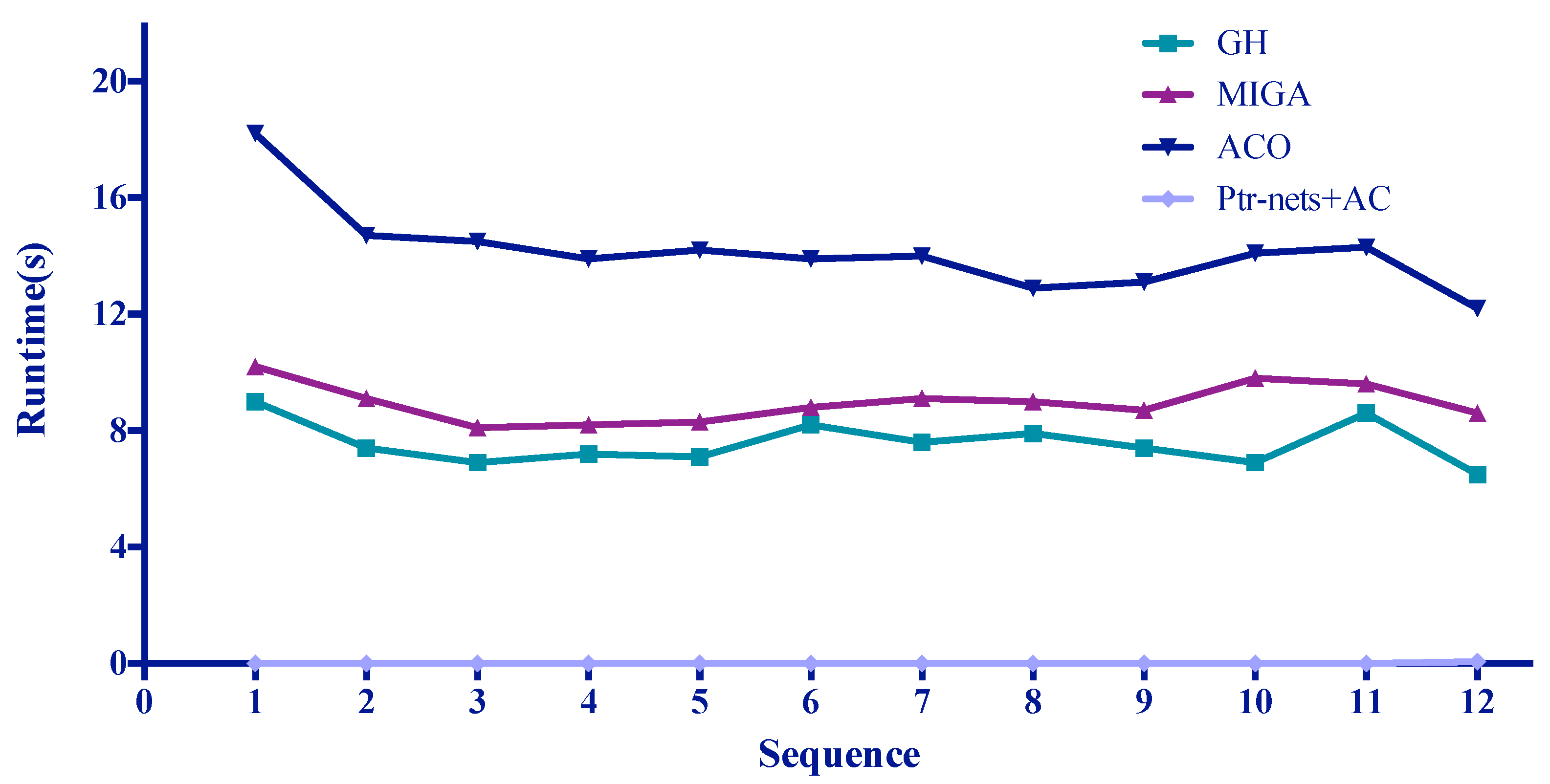
We note that the 12 original debris removal sequences were obtained through the mixed integer genetic algorithm (MIGA) [70]. The relevant parameters of ACO are set the same as those in the above dynamic TSP scenario. As for the parameters of MIGA, the population size and maximal iteration is set to 1000; the crossover probability and mutation probability are set to 0.8 and 0.2, respectively. Consequently, MIGA, ACO [53], GH and the Ptr-nets+AC algorithm are compared in Figure 9 and Figure 10. Figure 9 presents the comparison of the objective function, i.e., the flight cost of the spacecraft completing a sequence of debris removal, and Figure 10 illustrates the comparison of the computational time for the four algorithms.
Comparing the results from Table 11 and Figure 9 and Figure 10, it is found that the replanned flight cost by the Ptr-nets+AC algorithm is lower than that of other methods. The Ptr-nets+AC algorithm, based on the training and learning mechanism, can better capture the optimization information in complex environments and guide the generation of better debris removal schemes, while the MIGA, ACO, and heuristic algorithm still have much to improve on. Compared with the optimal debris removal sequence obtained by the Ptr-nets+AC and MIGA algorithm, it can be seen that most of the original debris removal sequences have been changed and only the 8th and 12th sequences remain the same, which are also the shortest debris chains among the 12 debris chains. To some extent, it indicates that MIGA is slightly weak in the larger-scale space debris removal mission planning problem. MIGA may fall into the local optimal solution easily, while the Ptr-nets+AC algorithm obtains global information from multiple rounds of training and learning, making it easier to realize global optimization. Moreover, it is presented that the Ptr-nets+AC algorithm consumes the minimum running time and can generate a high-quality debris removal solution almost instantaneously. Although it takes time to train the model, this method is valuable, especially for the research on large-scale debris removal missions.
Taking the No. 2 removal sequence as an example, it involves 11 space debris and 10 transfers, which is depicted in both Table 10 and Table 11. Figure 11 illustrates how the No. 2 removal sequence is changed after the replanning by the Ptr-nets+AC algorithm and Figure 12 illustrates the variation of the 10 transfer velocity increments for the removal sequence optimized by the MIGA and Ptr-nets+AC algorithm. As can be seen from the two figures, almost half of the removal sequence is rearranged and the velocity increments of the involved spacecraft transfers vary a lot. The velocity increments of 8 transfers are reduced by a large margin after the replanning and the total velocity increment is reduced by 544 m/s, which indicates the good performance of the Ptr-nets+AC algorithm in planning the active space debris removal missions.
Furthermore, by analyzing the two unchanged debris removal sequences (the 8th and 12th), the flight cost has also been reduced after replanning by the Ptr-nets+AC algorithm, which indicates that the Ptr-nets+AC algorithm can further optimize the rendezvous time between the spacecraft and the debris so as to obtain a better removal scheme. By comparing and analyzing the experimental results above, the effectiveness and superiority of the active debris removal mission planning method proposed in this paper are verified.
5. Conclusions
This paper proposes an active debris removal mission planning problem, devoted to optimizing the debris removal sequence, rendezvous time, and involved transfer trajectory, to generate an optimal debris removal plan to guide the mission process. According to the problem characteristics, the problem is decomposed into two layers. The outer layer is the debris removal sequence planning, which optimizes the debris removal sequence and rendezvous time. The inner layer is the transfer trajectory planning, which optimizes the transfer time and transfer velocity increment. Subsequently, a two-layer time-dependent TSP mathematical model is established. Two main solving methods for the ADR mission planning problem are proposed, including a DNN-based estimation method for approximating the optimal velocity increments of perturbed multiple-impulse rendezvous and an RL-based method for optimizing the sequence of debris removal and rendezvous time. Experimental results of different simulation scenarios have verified the effectiveness and superiority of the two proposed methods, respectively, indicating the good performance for solving the active debris removal mission planning problem.
For future perspectives, multiple spacecraft should be involved for future debris removal missions since a single spacecraft owns the restricted capability. Then, the mission allocation and coordination between multiple spacecraft are required to be further optimized for the ADR mission planning problem, which is worth further research.
Author Contributions
Conceptualization, Y.X. and X.L.; methodology, Y.X., X.L., Y.Z. (Yuehe Zhu) and Y.Z. (Yahui Zuo); validation, Y.X., X.L., Y.Z. (Yuehe Zhu), Y.Z. (Yahui Zuo) and L.H.; formal analysis, Y.X. and Y.Z. (Yahui Zuo); resources, X.L., R.H. and L.H.; data curation, Y.X.; writing—original draft preparation, Y.X.; writing—review and editing, X.L. and R.H.; visualization, Y.X.; supervision, X.L.; funding acquisition, X.L., R.H. and L.H. All authors have read and agreed to the published version of the manuscript.
Funding
This research was funded by the National Natural Science Foundation of China (Nos. 72001212).
Data Availability Statement
The data is included within the study for finding the results.
Conflicts of Interest
The authors declare no conflict of interest.
References
- Ledkov, A.; Aslanov, V. Review of contact and contactless active space debris removal approaches. Prog. Aerosp. Sci. 2022, 134, 194–206. [Google Scholar] [CrossRef]
- Kessler, D.J.; Cour-Palais, B.G. Collision frequency of artificial satellites the creation of a debris belt. J. Geophys. Res. 1978, 134, 2637–2646. [Google Scholar] [CrossRef]
- Federici, L.; Zavoli, A.; Colasurdo, G. A Time-Dependent TSP Formulation for the Design of an Active Debris Removal Mission using Simulated Annealing. arXiv 2019, arXiv:1909.10427. [Google Scholar]
- Bonnal, C.; Ruault, J.M.; Desjean, M.C. Active debris removal: Recent progress and current trends. Acta Astronaut. 2013, 85, 51–60. [Google Scholar] [CrossRef]
- Liou, J.C.; Johnson, N.L.; Hill, N.M. Controlling the growth of future LEO debris populations with active debris removal. Acta Astronaut. 2010, 66, 648–653. [Google Scholar] [CrossRef]
- Mayorova, V.I.; Shcheglov, G.A.; Stognii, M.V. Analysis of the space debris objects nozzle capture dynamic processed by a telescopic robotic arm. Acta Astronaut. 2021, 187, 259–270. [Google Scholar] [CrossRef]
- Zhan, B.; Jin, M.; Yang, G.; Zhang, C. A novel strategy for space manipulator detumbling a non-cooperative target with collision avoidance. Adv. Space Res. 2020, 66, 785–799. [Google Scholar] [CrossRef]
- Shan, M.; Guo, J.; Gill, E. An analysis of the flexibility modeling of a net for space debris removal. Adv. Space Res. 2019, 65, 1083–1094. [Google Scholar] [CrossRef]
- Aglietti, G.S.; Taylor, B.; Fellowes, S.; Salmon, T.; Retat, I.; Hall, A.; Chabot, C.; Pisseloup, A.; Cox, C.; Zarkesh, A. The active space debris removal mission RemoveDebris. Part 2: In orbit operations. Acta Astronaut. 2020, 168, 310–322. [Google Scholar] [CrossRef] [Green Version]
- Huang, P.; Wang, D.; Meng, Z.; Liu, Z. Post-capture attitude control for a tethered space robot–target combination system. Robotica 2015, 33, 898–919. [Google Scholar] [CrossRef]
- Zhao, Y.; Huang, P.; Zhang, F. Dynamic modeling and Super-Twisting Sliding Mode Control for Tethered Space Robot. Acta Astronaut. 2017, 143, 310–321. [Google Scholar] [CrossRef]
- Dudziak, R.; Tuttle, S.; Barraclough, S. Harpoon technology development for the active removal of space debris. Adv. Space Res. 2015, 56, 509–527. [Google Scholar] [CrossRef]
- Campbell, J.C.; Hughes, K.; Vignjevic, R.; Djordjevic, N.; Taylor, N.; Jardine, A. Development of modelling design tool for harpoon for active space debris removal. Int. J. Impact Eng. 2022, 166, 1–13. [Google Scholar] [CrossRef]
- Tamaki, Y.; Tanaka, H. Experimental study on penetration characteristics of metal harpoons with various tip shapes for capturing space debris. Adv. Space Res. Off. J. Comm. Space Res. 2022, 70, 310–323. [Google Scholar] [CrossRef]
- Holste, K.; Dietz, P.; Scharmann, S.; Keil, K.; Klar, P.J. Ion thrusters for electric propulsion: Scientific issues developing a niche technology into a game changer. Rev. Sci. Instruments 2020, 91, 1–55. [Google Scholar] [CrossRef]
- Alpatov, A.; Khoroshylov, S.; Bombardelli, C. Relative control of an ion beam shepherd satellite using the impulse compensation thruster. Acta Astronaut. 2018, 151, 543–554. [Google Scholar] [CrossRef]
- Bennett, T.; Schaub, H. Contactless electrostatic detumbling of axi-symmetric GEO objects with nominal pushing or pulling. Adv. Space Res. 2018, 62, 2977–2987. [Google Scholar] [CrossRef]
- Wilson, K.; Bengtson, M.; Schaub, H. Hybrid Method of Remote Sensing of Electrostatic Potential for Proximity Operations. In Proceedings of the 2020 IEEE Aerospace Conference, Big Sky, MT, USA, 7–14 March 2020. [Google Scholar]
- Fang, Y.; Pan, J. Effects of space-based nanosecond pulse laser driving centimeter-sized space debris in LEO. Opt.-Nternational J. Light Electron Opt. 2018, 180, 96–103. [Google Scholar] [CrossRef]
- Soulard, R.; Quinn, M.N.; Tajima, T.; Mourou, G. ICAN: A novel laser architecture for space debris removal. Acta Astronaut. 2014, 105, 192–200. [Google Scholar] [CrossRef]
- Kumar, R.; Sedwick, R.J. Despinning Orbital Debris Before Docking Using Laser Ablation. J. Spacecr. Rocket. 2015, 52, 1–6. [Google Scholar] [CrossRef]
- Aslanov, V.S. Gravitational Trap for Space Debris in Geosynchronous Orbit. J. Spacecr. Rocket. 2019, 56, 1277–1281. [Google Scholar] [CrossRef]
- Huang, P.; Zhang, F.; Chen, L.; Meng, Z.; Zhang, Y.; Liu, Z.; Hu, Y. A review of space tether in new applications. Nonlinear Dyn. 2018, 94, 1–19. [Google Scholar] [CrossRef]
- Yu, Y.; Yang, F.; Yue, H.; Lu, Y.; Zhao, H. Prospects of de-tumbling large space debris using a two-satellite electromagnetic formation. Adv. Space Res. 2021, 67, 1816–1829. [Google Scholar] [CrossRef]
- Hoffman, K.L.; Padberg, M.; Rinaldi, G. Traveling salesman problem. Encycl. Oper. Res. Manag. Sci. 2013, 1, 1573–1578. [Google Scholar]
- Cerf, M. Multiple Space Debris Collecting Mission—Debris Selection and Trajectory Optimization. J. Optim. Theory Appl. 2013, 156, 761–796. [Google Scholar] [CrossRef] [Green Version]
- Zuiani, F.; Vasile, M. Preliminary Design of Debris Removal Missions by Means of Simplified Models for Low-Thrust, Many-Revolution Transfers. Int. J. Aerosp. Eng. 2012, 2012, 836250. [Google Scholar] [CrossRef]
- Braun, V.; Lüpken, A.; Flegel, S.; Gelhaus, J.; Möckel, M.; Kebschull, C.; Wiedemann, C.; Vörsmann, P. Active debris removal of multiple priority targets. Adv. Space Res. 2013, 51, 1638–1648. [Google Scholar] [CrossRef]
- Zhang, N.; Zhang, Z.; Baoyin, H. Timeline Club:An optimization algorithm for solving multiple debris removal missions of the time-dependent traveling salesman problem model. Astrodynamics 2022, 6, 219–234. [Google Scholar] [CrossRef]
- Li, H.; Chen, S.; Baoyin, H. J2-Perturbed Multitarget Rendezvous Optimization with Low Thrust. J. Guid. Control Dyn. 2018, 41, 796–803. [Google Scholar] [CrossRef]
- Olympio, J.T.; Frouvelle, N. Space debris selection and optimal guidance for removal in the SSO with low-thrust propulsion. Acta Astronaut. 2014, 99, 263–275. [Google Scholar] [CrossRef]
- Barea, A.; Urrutxua, H.; Cadarso, L. Large-scale object selection and trajectory planning for multi-target space debris removal missions. Acta Astronaut. 2020, 170, 289–301. [Google Scholar] [CrossRef]
- Madakat, D.; Morio, J.; Vanderpooten, D. Biobjective planning of an active debris removal mission. Acta Astronaut. 2013, 84, 182–188. [Google Scholar] [CrossRef]
- Olive, X.; Berend, N. Bi-objective optimization of a multiple-target active debris removal mission. Acta Astronaut. 2016, 122, 324–335. [Google Scholar]
- Forrest, S. Genetic algorithms. ACM Comput. Surv. (CSUR) 1996, 28, 77–80. [Google Scholar] [CrossRef]
- Hwang, C.R. Simulated annealing. In Simulated Annealing: Theory and Applications; Laarhoven, P.J.M., Aarts, E.H.L., Eds.; Kluwer Academic Publishers: Boston, MA, USA, 1987; pp. 21–40. [Google Scholar]
- Lewis, O.L.; Zhang, S.; Guy, R.D.; Del Alamo, J.C. Coordination of contractility, adhesion and flow in migrating Physarum amoebae. J. R Soc. Interface 2015, 12, 20141359. [Google Scholar] [CrossRef] [Green Version]
- Guy, R.D.; Lewis, O.L.; Zhang, S.; del Alamo, J.C. Coordination of Contractility, Adhesion and Flow in Migrating Physarum Amoebae: Experiments and Modeling. In Proceedings of the 9th EAI International Conference on Bio-inspired Information and Communications Technologies (Formerly BIONETICS), New York City, NY, United States, 3–5 December 2016. [Google Scholar]
- Eberhart, R.; Kennedy, J. A new optimizer using particle swarm theory. In Proceedings of the Mhs95 Sixth International Symposium on Micro Machine and Human Science, Nagoya, Japan, 4–6 October 1995. [Google Scholar]
- Dorigo, M.; Maniezzo, V. Ant system: Optimization by a colony of cooperating agents. IEEE Trans. SMC-Part B 1996, 26, 29–41. [Google Scholar] [CrossRef] [Green Version]
- Murakami, J.; Hokamoto, S. Approach for Optimal Multi-Rendezvous Trajectory Design for Active Debris Removal. In Proceedings of the 61st International Astronautical Congress, Prague, Czech Republic, 27 September–1 October 2010. [Google Scholar]
- Liu, Y.; Yang, J.; Wang, Y.; Pan, Q.; Yuan, J. Multi-objective optimal preliminary planning of multi-debris active removal mission in LEO. Sci. China Inf. Sci. 2017, 60, 072202. [Google Scholar] [CrossRef]
- Chen, Y.; Bai, Y.; Zhao, Y.; Wang, Y.; Chen, X. Optimal mission planning of active space debris removal based on genetic algorithm. IOP Conf. Ser. Mater. Sci. Eng. 2020, 715, 012025. [Google Scholar] [CrossRef]
- Missel, J.; Mortari, D. Path optimization for Space Sweeper with Sling-Sat: A method of active space debris removal. Adv. Space Res. 2013, 52, 1339–1348. [Google Scholar] [CrossRef]
- Medioni, L.; Gary, Y.; Monclin, M.; Oosterhof, C.; Pierre, G.; Semblanet, T.; Comte, P.; Nocentini, K. Trajectory optimization for multi-target Active Debris Removal missions. ASR 2022, in press. [Google Scholar]
- Carlo, M.; Martin, J.R.; Vasile, M. Automatic trajectory planning for low-thrust active removal mission in low-earth orbit. Adv. Space Res. 2016, 59, 1234–1258. [Google Scholar] [CrossRef] [Green Version]
- Jing, Y.; Chen, X.Q.; Chen, L.H. Biobjective planning of GEO debris removal mission with multiple servicing spacecrafts. Acta Astronaut. 2014, 105, 311–320. [Google Scholar] [CrossRef]
- Mohammadi-Dehabadi, A.A.; Daneshjou, K.; Bakhtiari, M. Mission planning for on-orbit servicing through multiple servicing satellites: A new approach. Adv. Space Res. Off. J. Comm. Space Res. 2017, 60, 1148–1162. [Google Scholar]
- Stuart, J.; Howell, K.; Wilson, R. Application of multi-agent coordination methods to the design of space debris mitigation tours. Adv. Space Res. 2015, 57, 911–928. [Google Scholar] [CrossRef]
- Shen, H.X.; Zhang, T.-J.; Casalino, L.; Pastrone, D. Optimization of Active Debris Removal Missions with Multiple Targets. J. Spacecr. Rocket. 2018, 55, 181–189. [Google Scholar] [CrossRef]
- Zhang, T.; Shen, H.; Li, H.; Li, J. Ant Colony Optimization based design of multiple-target active debris removal mission. Trans. Jpn. Soc. Aeronaut. Space Sci. 2018, 61, 201–210. [Google Scholar] [CrossRef] [Green Version]
- Li, H.; Baoyin, H. Optimization of Multiple Debris Removal Missions Using an Evolving Elitist Club Algorithm. IEEE Trans. Aerosp. Electron. Syst. 2020, 56, 773–784. [Google Scholar] [CrossRef]
- Zhu, Y.H. Flight Sequence Planning Method for Large-Scale-Object Visiting Mission. Ph.D. Thesis, National University of Defense Technology, Changsha, China, 2022. [Google Scholar]
- Lucena, A. Time-dependent traveling salesman problem–the deliveryman case. Networks 1990, 20, 753–763. [Google Scholar] [CrossRef]
- Zhu, Y.; Luo, Y.; Zhang, J. Packing programming of space station spacewalk events based on bin packing theory and differential evolution algorithm. In Proceedings of the 2016 IEEE Congress on Evolutionary Computation (CEC), Vancouver, BC, Canada, 24–29 July 2016; pp. 877–884. [Google Scholar]
- Boggs, P.T.; Tolle, J.W. Sequential quadratic programming. Acta Numer. 1995, 4, 1–51. [Google Scholar] [CrossRef] [Green Version]
- Montavon, G.; Samek, W.; Müller, K.R. Methods for interpreting and understanding deep neural networks. Digit. Signal Process. 2018, 73, 1–15. [Google Scholar] [CrossRef]
- Riedmiller, M.; Lernen, A. Multi Layer Perceptron; Machine Learning Lab Special Lecture; University of Freiburg: Breisgau, Germany, 2014; pp. 7–24. [Google Scholar]
- Karlik, B.; Olgac, A.V. Performance Analysis of Various Activation Functions in Generalized MLP. Int. J. Artif. Intell. Expert Syst. 2010, 1, 111–122. [Google Scholar]
- Dokkyun, Y.; Jaehyun, A.; Sangmin, J. An Effective Optimization Method for Machine Learning Based on ADAM. Comput. Sci. 2020, 10, 1073–1092. [Google Scholar]
- Ketkar, N. Keras. In Deep Learning with Python; Welmoed, S., Todd, G., Eds.; SPi Global: New York, NY, USA, 2017; pp. 97–112. [Google Scholar]
- Abadi, M.; Agarwal, A.; Barham, P.; Brevdo, E.; Chen, Z.; Citro, C.; Corrado, G.S.; Davis, A.; Dean, J.; Devin, M. TensorFlow: Large-Scale Machine Learning on Heterogeneous Distributed Systems. In Proceedings of the 12th USENIX conference on Operating Systems Design and Implementation, Savannah, GA, USA, 2–4 November 2016. [Google Scholar]
- Vinyals, O.; Fortunato, M.; Jaitly, N. Pointer networks. In Proceedings of the 28th International Conference on Neural Information Processing Systems, Montreal, Canada, 7–12 December 2015. [Google Scholar]
- Sutskever, I.; Vinyals, O.; Le, Q.V. Sequence to Sequence Learning with Neural Networks. In Proceedings of the 27th International Conference on Neural Information Processing Systems, Montreal, Canada, 8–13 December 2014. [Google Scholar]
- Grondman, I.; Busoniu, L.; Lopes, G.A.; Babuska, R. A survey of actor-critic reinforcement learning: Standard and natural policy gradients. IEEE Trans. Syst. Man, Cybern. Part C 2012, 42, 1291–1307. [Google Scholar] [CrossRef] [Green Version]
- Bello, I.; Pham, H.; Le, Q.V.; Norouzi, M.; Bengio, S. Neural Combinatorial Optimization with Reinforcement Learning. arXiv 2016, arXiv:1611.09940. [Google Scholar]
- Wang, G.P.; Duan, M.; Niu, C.Y. Stochastic gradient descent algorithm based on convolution neural network. Comput. Eng. Des. 2018, 39, 441–445. [Google Scholar]
- HE, B.; Li, X.; Zheng, J. Scenario analysis of wind power output based on LHS and BR. Electr. Power Eng. Technol. 2020, 39, 213–219. [Google Scholar]
- Macdonald, M.; McKay, R.; Vasile, M.; Frescheville, F.B.d. Extension of the sun-synchronous orbit. J. Guid. Control. Dyn. 2010, 33, 1935–1940. [Google Scholar] [CrossRef] [Green Version]
- Luo, Y.Z.; Zhu, Y.H. GTOC9: Results from the National University of Defense Technology (team NUDT). Acta Futur. 2018, 11, 37–47. [Google Scholar]
- Luo, Y.Z.; Li, H.Y.; Tang, G.J. Hybrid Approach to Optimize a Rendezvous Phasing Strategy. J. Guid. Control Dyn. 2007, 30, 185–191. [Google Scholar] [CrossRef]
- Hongxin, S.; Tianjiao, Z.; Anyi, H.; Zhao, L. GTOC 9: Results from the Xi’an Satellite Control Center (team XSCC). Acta Futur. 2018, 11, 49–55. [Google Scholar]
- Edelbaum, T.N. Propulsion Requirements for Controllable Satellites. Ars J. 1961, 31, 1079–1089. [Google Scholar] [CrossRef]
- GTOC 9—The Kessler Run. Available online: https://sophia.estec.esa.int/gtoc_portal/?page_id=814 (accessed on 21 February 2023).
Figure 1.
Decomposition of the active space debris removal mission planning problem.

Figure 2.
A static target visiting sequence and a time-dependent rendezvous sequence for moving targets.
Figure 2.
A static target visiting sequence and a time-dependent rendezvous sequence for moving targets.

Figure 3.
A time-dependent moving target rendezvous sequence with time discretization.

Figure 4.
Framework of the active debris removal mission planning method based on machine learning.

Figure 5.
Variation trend of the right ascension of the ascending node () between the departure body and the rendezvous target for three types of perturbed multiple-impulse rendezvous.
Figure 5.
Variation trend of the right ascension of the ascending node () between the departure body and the rendezvous target for three types of perturbed multiple-impulse rendezvous.

Figure 6.
Solving framework of the estimation methods for perturbed multiple-impulse rendezvous.

Figure 7.
Improved pointer network with dynamic information.

Figure 8.
The optimal travel route generated by the Ptr-nets+AC algorithm.

Figure 9.
Comparison of the optimal replanned debris removal plan for MIGA, ACO, GH, and the Ptr-nets+AC algorithm.
Figure 9.
Comparison of the optimal replanned debris removal plan for MIGA, ACO, GH, and the Ptr-nets+AC algorithm.

Figure 10.
Comparison of the running time for GH, MIGA, ACO, and Ptr-nets+AC algorithm to plan the 12 space debris removal sequences.
Figure 10.
Comparison of the running time for GH, MIGA, ACO, and Ptr-nets+AC algorithm to plan the 12 space debris removal sequences.

Figure 11.
Comparison between the original and replanned solutions for the No. 2 debris removal sequence generated by the MIGA and Ptr-nets+AC algorithm, respectively.
Figure 11.
Comparison between the original and replanned solutions for the No. 2 debris removal sequence generated by the MIGA and Ptr-nets+AC algorithm, respectively.

Figure 12.
Variation of the 10 transfer velocity increments for the No. 2 debris removal sequence optimized by the MIGA and Ptr-nets+AC algorithm.
Figure 12.
Variation of the 10 transfer velocity increments for the No. 2 debris removal sequence optimized by the MIGA and Ptr-nets+AC algorithm.


Table 1.
The ranges of the six orbital elements.
| Parameter | a (km) | e | i (deg) | (deg) | w (deg) | m (deg) |
|---|---|---|---|---|---|---|
| Value |
Table 2.
Parameters of the experiment for estimation of transfer impulse velocity increment.
| Parameter | Description | Value |
|---|---|---|
| Population size for DE algorithm | 100 | |
| Maximal iteration for DE algorithm | 1000 | |
| Maximum transfer time | 30 days | |
| Maximum allowable position error for rendezvous | 1 m | |
| Maximum allowable velocity error for rendezvous | 0.01 m/s | |
| The number of the initial training samples for each transfer type | 5000 | |
| The number of the terminal training samples for each transfer type | 10,000 | |
| The number of the testing samples for each transfer type | 1000 | |
| Hidden layers | 2 |
Table 3.
Potential learning features for estimating optimal velocity increments.
| Feature | Description |
|---|---|
| Semi-major axis of the departure body and rendezvous target | |
| Eccentricities of the departure body and rendezvous target | |
| Inclinations of the departure body and rendezvous target | |
| Difference between initial RAAN of the departure body and initial RAAN of the rendezvous target | |
| Difference between terminal RAAN of the departure body and terminal RAAN of the rendezvous target | |
| Difference between initial RAAN of the departure body and terminal RAAN of the rendezvous target | |
| RAAN variation rates of the departure body and rendezvous target | |
| Initial and terminal phase differences between the departure body and rendezvous target | |
| Transfer time |
Table 4.
Selected learning features for the three types of perturbed multiple-impulse transfer.
| Type | Feature Combination | MRE |
|---|---|---|
| closing | 5.98% | |
| intersecting | 5.95% | |
| separating | 5.51% |
Table 5.
MREs of the estimation for the two analytical methods and DNN-based method.
| Type | Closing | Intersecting | Separating |
|---|---|---|---|
| Edelbaum-based | 21.96% | 16.38% | 22.43% |
| Gauss-based | 20.37% | 17.93% | 5.95% |
| DNN-based | 2.56% | 2.29% | 2.64% |
Table 6.
The initial location and the terminal location of 15 cities.
| City | Initial Location | Terminal Location |
|---|---|---|
| 1 | ||
| 2 | ||
| 3 | ||
| 4 | ||
| 5 | ||
| 6 | ||
| 7 | ||
| 8 | ||
| 9 | ||
| 10 | ||
| 11 | ||
| 12 | ||
| 14 | ||
| 15 |
Table 7.
Parameter settings in the training process for active debris removal planning.
| Parameter | Description | Value |
|---|---|---|
| The number of the training samples | 3000 | |
| The number of the testing samples | 1000 | |
| Mini batch size | 128 | |
| Learning rate | ||
| Baseline decay parameter | 0.99 | |
| norm | 1.0 | |
| Embedding dimension | 128 | |
| Hidden unit size | 128 | |
| Time discretization interval | 3 min |
Table 8.
Optimal traveling route for the heuristic algorithm, ant colony optimization, and the Ptr-nets+ AC algorithm.
Table 8.
Optimal traveling route for the heuristic algorithm, ant colony optimization, and the Ptr-nets+ AC algorithm.
| Algorithm | Number | Optimal Travel Route | Total Length | Runtime |
|---|---|---|---|---|
| Ptr-nets+AC | 1 | 864.32 | 0.003 s | |
| 2 | 864.32 | 0.002 s | ||
| 3 | 864.32 | 0.003 s | ||
| ACO | 1 | 879.89 | 5.6 s | |
| 2 | 879.42 | 6.2 s | ||
| 3 | 879.44 | 5.9s | ||
| GH | 1 | 950.09 | 2.3 s | |
| 2 | 950.09 | 3.4 s | ||
| 3 | 950.09 | 2.7 s |
Table 9.
The orbital elements of the partial space debris.
| Debris | Time | a | e | i | w | m | |
|---|---|---|---|---|---|---|---|
| Number | (MJD2000) | (m) | (rad) | (rad) | (rad) | (rad) | |
| 0 | 21,947.64964 | 7,165,739.682 | 0.001487 | 1.708495 | 5.425149 | 0.518965 | 3.220888 |
| 1 | 22,167.21634 | 7,119,482.457 | 0.016819 | 1.719032 | 4.030232 | 2.249735 | 4.880728 |
| 2 | 21,971.81499 | 7,159,621.255 | 0.003793 | 1.695100 | 2.928707 | 4.493324 | 6.243761 |
| 3 | 22,169.54327 | 7,110,511.243 | 0.006666 | 1.694290 | 0.623365 | 3.411909 | 4.771420 |
| 4 | 22,052.22244 | 7,102,000.094 | 0.001830 | 1.749873 | 2.622564 | 2.397072 | 3.132921 |
| 5 | 21,974.98101 | 7,173,465.035 | 0.008501 | 1.725002 | 4.716882 | 2.987324 | 5.494481 |
| 6 | 22,148.09259 | 7,058,041.710 | 0.008723 | 1.720674 | 3.574643 | 4.981435 | 4.195619 |
| 7 | 22,142.82488 | 7,059,602.053 | 0.002493 | 1.706914 | 1.455986 | 4.302093 | 5.348153 |
| 8 | 22,128.71786 | 7,134,323.940 | 0.016272 | 1.744527 | 0.132978 | 5.838210 | 5.562178 |
| 9 | 22,037.55936 | 7,147,207.980 | 0.008008 | 1.705436 | 3.378731 | 1.276019 | 5.223427 |
| 10 | 22,187.76363 | 7,162,215.176 | 0.002402 | 1.717952 | 2.604417 | 1.894280 | 4.384844 |
| 11 | 22,091.993 | 7,232,507.650 | 0.001177 | 1.706631 | 3.051655 | 1.707654 | 3.357483 |
Table 10.
Twelve removal sequences for the 123 debris.
| Number | Start Time | Terminal Time | Debris Removal Sequence | Objective |
|---|---|---|---|---|
| 1 | 23,517.00 | 23,811.52 | 24.19 | |
| 2 | 23,893.80 | 24,092.29 | 8.87 | |
| 3 | 24,122.30 | 24,427.74 | 6.55 | |
| 4 | 24,461.50 | 24,660.15 | 8.66 | |
| 5 | 24,785.00 | 24,975.41 | 28.61 | |
| 6 | 25,006.00 | 25,198.32 | 8.19 | |
| 7 | 25,281.60 | 25,454.87 | 16.56 | |
| 8 | 25,555.40 | 25,669.64 | 16.93 | |
| 9 | 25,702.40 | 25,860.22 | 11.71 | |
| 10 | 25,912.74 | 26,055.85 | 7.23 | |
| 11 | 26,087.53 | 26,262.18 | 10.28 | |
| 12 | 26,292.26 | 26,381.58 | 5.02 |
Table 11.
The 12 replanned debris removal sequences by the Ptr-nets+AC algorithm.
| Number | Replanned Debris Removal Sequence | Initial Cost | New Cost |
|---|---|---|---|
| 1 | 24.19 | 13.08 | |
| 2 | 8.87 | 4.36 | |
| 3 | 6.55 | 3.04 | |
| 4 | 8.66 | 5.71 | |
| 5 | 28.61 | 20.8 | |
| 6 | 8.19 | 4.57 | |
| 7 | 16.56 | 10.52 | |
| 8 | 16.93 | 12.6 | |
| 9 | 11.71 | 7.71 | |
| 10 | 7.23 | 4.8 | |
| 11 | 10.28 | 7.11 | |
| 12 | 5.02 | 3.78 |
Disclaimer/Publisher’s Note: The statements, opinions and data contained in all publications are solely those of the individual author(s) and contributor(s) and not of MDPI and/or the editor(s). MDPI and/or the editor(s) disclaim responsibility for any injury to people or property resulting from any ideas, methods, instructions or products referred to in the content. |
© 2023 by the authors. Licensee MDPI, Basel, Switzerland. This article is an open access article distributed under the terms and conditions of the Creative Commons Attribution (CC BY) license (https://creativecommons.org/licenses/by/4.0/).
Share and Cite
MDPI and ACS Style
Xu, Y.; Liu, X.; He, R.; Zhu, Y.; Zuo, Y.; He, L. Active Debris Removal Mission Planning Method Based on Machine Learning. Mathematics 2023, 11, 1419. https://0-doi-org.brum.beds.ac.uk/10.3390/math11061419
AMA Style
Xu Y, Liu X, He R, Zhu Y, Zuo Y, He L. Active Debris Removal Mission Planning Method Based on Machine Learning. Mathematics. 2023; 11(6):1419. https://0-doi-org.brum.beds.ac.uk/10.3390/math11061419
Chicago/Turabian StyleXu, Yingjie, Xiaolu Liu, Renjie He, Yuehe Zhu, Yahui Zuo, and Lei He. 2023. "Active Debris Removal Mission Planning Method Based on Machine Learning" Mathematics 11, no. 6: 1419. https://0-doi-org.brum.beds.ac.uk/10.3390/math11061419
Note that from the first issue of 2016, this journal uses article numbers instead of page numbers. See further details here.