Super-Resolution Reconstruction-Based Plant Image Classification Using Thermal and Visible-Light Images

Abstract

Few studies have been conducted on thermal plant images. This is because of the difficulty in extracting and analyzing various color-related patterns and features from the plant image obtained using a thermal camera, which does not provide color information. In addition, the thermal camera is sensitive to the surrounding temperature and humidity. However, the thermal camera enables the extraction of invisible patterns in the plant by providing external and internal heat information. Therefore, this study proposed a novel plant classification method based on both the thermal and visible-light plant images to exploit the strengths of both types of cameras. To the best of our knowledge, this study is the first to perform super-resolution reconstruction using visible-light and thermal plant images. Furthermore, a method to improve the classification performance through generative adversarial network (GAN)-based super-resolution reconstruction was proposed. Through the experiments using a self-collected dataset of thermal and visible-light images, our method shows higher accuracies than the state-of-the-art methods.

1. Introduction

There are many studies on plant classification based on images captured with visible-light cameras. However, in order to obtain external and internal patterns and features of a plant that cannot be obtained with visible-light cameras, thermal cameras have recently begun to be used. However, studies on plant image classification using thermal cameras are scarce. A visible-light camera is sensitive to light and may produce low-quality images in a low-illumination environment or because of illumination change. Further, a thermal camera, which is sensitive to temperature and humidity, produces low-quality images owing to radiation emitted from or reflected by the various objects in the surroundings. Considering these challenges and strengths of the visible-light and thermal cameras, this study examined the use of both thermal and visible-light plant images. In addition, super-resolution reconstruction (SRR) was performed to establish a classification method with improved performance compared to the previous studies. This is the first study to use visible-light and thermal images to perform SRR. The proposed method is described in detail in Section 3. Additionally, various SRR and classification experiments were conducted by using a self-collected thermal and visible-light plant image database. The novelty and innovations of this study are as follows:

−

Most previous studies focused on plant SRR based on visible-light images; however, no study exists on thermal-based images. This study examined SRR using thermal and visible-light plant images for the first time. In addition, this study proposed an SRR-based multiclass classification method using thermal and visible-light plant images.

−

In this study, a novel method of a plant super-resolution (PlantSR) network was proposed with low-resolution (LR) thermal images (200 × 200 × 1) or LR visible-light images (200 × 200 × 3) as the input. In addition, a new residual blocks-in-residual block (RBRB) was employed in the structures of PlantSR and plant classification, thereby increasing the accuracy of plant classification.

−

In this study, a novel method of a plant multiclass classification (PlantMC) network was proposed using high-resolution (HR) thermal images and HR visible-light images as the input. To reduce the processing time of the PlantMC network, the input images, HR thermal images (600 × 600 × 1) and HR visible-light images (600 × 600 × 3) were cropped and converted into images with sizes of 200 × 200 × 25 and 200 × 200 × 75, respectively, through channel-wise concatenation. In addition, the accuracy of plant classification was improved using a new RBRB in the structure of PlantMC.

−

The PlantSR and PlantMC models proposed in the study and the self-collected thermal and visible-light plant image database were made available to other researchers [1].

The existing classification studies based on plant images can be categorized into plant image classification with SRR and plant image classification without SRR, where only visible-light images are used by the previous plant image-based SSR studies. Detailed explanations of the relevant works are presented in Section 2. Further, the experimental methods employed in this study are described in Section 3. The results and analysis of the experiments employing such methods are presented in Section 4. Finally, the discussion and conclusion are provided in Section 5 and Section 6, respectively.

2. Related Works

2.1. Plant Image Classification without Super-Resolution Reconstruction

This subsection discusses the existing plant image classification studies without SRR. These studies were divided into three parts: visible-light image-based, thermal image-based and thermal- and visible-light image-based studies.

2.1.1. Visible-Light Image-Based Studies

Existing plant visible-light image-based classification studies are as follows. A study on crop disease classification [2] was conducted using the PlantDoc database and AAR network. Another method of crop disease classification [3] was performed using the PlantDoc database and DenseNet-121 model. A different study on crop disease classification [4] employed the PlantDoc database and OMNCNN network to conduct the experimentation. A demonstration of crop and crop disease classification [5] utilized the PlantDoc database and five different deep learning methods (MobileNetV1, MobileNetV2, NASNetMobile, DenseNet121 and Xception). Another study on crop and crop disease classification [6] proposed a trilinear convolutional neural network model (T-CNN), while conducting various experiments using PlantVillage [7], PlantDoc [8] databases and pre-trained model with ImageNet. A prior study on plant image classification [9] was conducted using two models: periodic implicit generative adversarial networks (PI-GANs) and PI-CNN. The study employed four datasets (PlantVillage, PlantDoc, Fruits-360 and Plants) and performed various experiments while reducing the number of frames in the video. Augmentation was performed using PI-GAN and classification was conducted using PI-CNN.

Although these studies used visible-light cameras, the light-sensitive visible-light cameras have the disadvantage of producing low-quality images due to shadow, low illumination, illumination change and ambient light and its reflection. In addition, visible-light cameras cannot be used to capture images at night without light. These limitations motivated the proposal of thermal plant image-based methods, which are explained in Section 2.1.2.

2.1.2. Thermal Image-Based Studies

A study on plant image and disease image classification [10] proposed the PlantDXAI model, and various experiments were conducted using a paddy crop dataset and self-collected dataset. In this study, the CNN-16 network was used to perform plant classification, and class activation map and discriminator were additionally employed in the training phase to improve the performance of CNN-16 for disease classification.

These studies only used thermal cameras, which are sensitive to temperature and humidity and, therefore, produce low-quality images owing to radiation emitted and reflected by various objects in the environment. To address these challenges, thermal and visible-light plant image-based methods have been explored, as introduced in Section 2.1.3.

2.1.3. Thermal and Visible-Light Image-Based Studies

In a previous study on plant image classification [11], a classification method based on both thermal and visible-light images was proposed. According to the method, binary classification was performed via simultaneous use of thermal and visible-light images. In addition, the thermal image and stereo visible-light images were obtained for the study from three types of camera sensors: thermal and dual visible-light cameras. By integrating the three types of images, the accuracy of classifying them into healthy and diseased plant images increased. Further, binary classification (healthy or diseased) was performed by processing the features extracted with manual feature extraction methods through analysis of variance (ANOVA) [12] and support vector machine (SVM) [13]. However, such a method increases the computation time and complexity of the system, owing to the simultaneous use of three types of cameras. Moreover, this method employs manual feature extraction methods and, thus, appropriate features cannot be extracted. In addition, only binary classification was performed using this method and various plant images were not recognized. A study on plant image classification [14] was conducted using nonaligned thermal and visible-light images. It proposed PlantCR and performed multiclass classification by considering visible-light and thermal images as the model input and integrating the two types of images inside the model.

However, the classification performance is limited by the LR images. To overcome this challenge, plant image classification methods based on plant image SSR were developed, as further explained in Section 2.2.

2.2. Plant Image Classification with Super-Resolution Reconstruction

In this section, existing plant image classification studies with SRR are explained. A previous study [15] demonstrated SRR and conducted plant disease classification using HR images produced with SRR. Each of the LR-, HR- and SRR-produced HR images are used to perform plant disease classification and the results were compared. In addition, the study compared the performance of the super-resolution convolutional neural network (SRCNN) with those of cubic, bicubic, lanczos and nearest neighbor (NN). Further, AlexNet was used for disease classification. Another study [16] demonstrated SRR and performed plant disease diagnosis using HR images produced with SRR. In the study, GAN [17] was used to achieve SRR, and 23 residual-in-residual dense blocks (RRDBs) were employed by the generator network. In addition, multiclass classification was executed using CNN_Diag as the disease classification method.

However, these studies used visible-light cameras, and there are no studies on SRR using thermal plant images. In addition, there are very few multiclass classification studies that have used thermal images, including the studies introduced in Section 2. However, no study was conducted for both SRR and classification using thermal and visible-light images. Such a gap motivates this study to demonstrate multiclass classification using thermal and visible-light plant images and conduct SRR to further improve the accuracy. The proposed methods, PlantSR and PlantMC, are thoroughly explained in Section 3.

The aforementioned studies are summarized in

Table 1. Summary of existing classification and SRR studies on plant image databases.

Categories	Modalities	Tasks	Methods	Advantages	Disadvantages
Classification without SRR	Visible-light image-based	Multiclass classification	AAR network [2], DenseNet-121 [3], OMNCNN [4], CNNs [5], T-CNN [6], and PI-CNN [9]	− Provides high-quality (HQ) image in both day and high illumination environment − Provides color information − Extracts features automatically − Considers multiclass problem	− Provides dark image in a nighttime or low illumination environment − Provides low-quality (LQ) image in both day and high illumination environment owing to shadow, illumination change, ambient light, and its reflection.
	Thermal image-based	Multiclass classification	PlantDXAI [10]	− Provides thermal information − Extracts features automatically − Considers multiclass problem	− Does not provide color information − Sensitive to temperature and humidity of the environment
	Thermal and visible-light images-based	Binary classification	SVM [11]	− Provides HQ image in both day and high illumination environment − Provides color and thermal information	− Very challenging to extract appropriate features − Does not consider multiclass problem − Computationally expensive owing to use of three camera sensors
		Multiclass classification	PlantCR [14]	− Provides HQ image in both day and high illumination environment − Provides color and thermal information − Extracts features automatically − Considers multiclass problem	Computationally expensive owing to use of two camera sensors
Classification with SRR	Visible-light image-based	Multiclass classification	Modified SRCNN + AlexNet [15], GAN-based SRR + CNNDiag [16]	− Provides HR and HQ image in both day and high illumination environment − Provides color information − Higher performance by using classification with SRR − Extracts features automatically − Considers multiclass problem	− Provides dark image in nighttime or low illumination environment − Provides LQ image in both day and high illumination environment owing to shadow, illumination change, ambient light, and its reflection.
	Thermal and visible-light images-based	Multiclass classification	PlantSR + PlantMC (Proposed method)	− Provides HR and HQ image in both day and high illumination environment − Provides thermal and color information − Higher performance by using classification with SRR − Extracts features automatically − Considers multiclass problem	Computationally expensive owing to use of two camera sensors

for comparison.

3. Materials and Methods

3.1. Overall Procedure of the Proposed Method

In this section, the method proposed by this study is explained in detail. A flowchart describing the method is provided in Figure 1. As is evident, the plant thermal and visible-light images are considered as input and categorized into twenty-eight classes by integrating the extracted features. To improve the classification performance, the LR input image of 200 × 200 dimensions was expanded into a 600 × 600 HR image through PlantSR. Subsequently, the HR image was used as input for PlantMC by cropping it into an image of 200 × 200 dimensions to reduce the processing time of classification. Detailed explanations of preprocessing are provided in Section 3.2. In addition, detailed descriptions of the proposed structure of PlantSR and PlantMC networks are presented in Section 3.3 and Section 3.4, respectively, using tables and figures. In addition, the dimensions of input and output images and parameters used for the structures are explained.

3.2. Preprocessing

In this section, the preprocessing introduced in Figure 1, which involves cropping the HR image of 600 × 600 dimensions into a 200 × 200 × N image, is explained in detail. Examples of preprocessing thermal and visible-light images are shown in Figure 2 and Figure 3, with Figure 2 focusing on further details. The preprocessing procedure entails cropping the input image into 200 × 200 dimensions by shifting it from left to right and top to bottom. Twenty-five cropped images (200 × 200 × 1) were then used to produce one 200 × 200 × 25 image (Figure 2) through channel-wise concatenation. In the shifting process, the image was cropped while overlapping at half the size (p = 100) of the output image (s = 200) to not overlook the image pattern. In the case of the visible-light image, the number of channels is 3, which becomes 75 after the preprocessing operation (Figure 3). The output images produced in Figure 2 and Figure 3 are used as input to the proposed PlantMC. Simply, in the preprocessing stage, we reduce the size of input images to decrease the processing time. To achieve that, an input image is sliced into smaller images and the images are combined into a single image but with more channels, as shown in Figure 2 and Figure 3. In other words, we reduce the spatial size but increase the number of channels in an image. We confirmed that the preprocessing operation decreases the processing time, as shown in Section 4.4. Moreover, we can also confirm that the preprocessing operation does not decrease the accuracy of the proposed method, as shown in experiments in Section 4.2.

3.3. Detailed Structure of the Proposed PlantSR Network

The dimensions of input and output images in the generator network are 200 × 200 × X and 600 × 600 × X, respectively, where X represents the number of channels, which is one for the thermal image and three for the visible-light image.

Table 2. Description of the generator network of PlantSR.

Layer#	Layer Type	Filter#	Parameter#	Layer Connection
1	input layer	0	0	input
2	group_1	128	741,760	input layer
3	Up3	0	0	group_1
4	group_2	64	258,560	Up3
5	conv2d (tanh)	X	1,731	group_2
	Total number of trainable parameters: 1,002,051

and

Table 3. Description of the discriminator network of PlantSR.

Layer#	Layer Type	Filter#	Parameter#	Layer Connection
1	input layer	0	0	input
2	group_1	64	334,400	input layer
3	group_2	64	369,536	group_1
4	LReLU	0	0	group_2
5	FC (sigmoid)	Class#	1,382,977	LReLU
	Total number of trainable parameters: 2,086,913

present the descriptions of the generator and discriminator networks, respectively. As shown in Table 2, Table 3,

Table 4. Group layer of generator network.

Times	Layer Type	Layer Connection
1	input layer	input
2	conv2d	input layer
1	RBRB	conv2d

,

Table 5. Group layer of discriminator network.

Times	Layer Type	Layer Connection
1	input layer	input
2	conv2d	input layer
1	max_pool	conv2d
2	RBRB	max_pool

,

Table 6. Description of RBRB.

Layer Type	Layer Connection
input layer	input
res_block_1	input layer
res_block_2	res_block_1
add	res_block_2 & input layer

and

Table 7. Description of a residual block.

Layer Type	Layer Connection
input layer	input
conv2d_1	input layer
prelu	conv2d_1
conv2d_2	prelu
add	conv2d_2 & input layer

, input (input image), input layer, group layer (group), up-sampling layer (Up3), convolution layer (conv2d), activation layers (tanh and sigmoid), leaky rectified linear unit (LReLU), fully connected layer (FC), RBRB layer (RBRB), max pooling layer (max_pool), residual block (res_block), parametric rectified linear unit (prelu) and additional operation layer (add) were employed to construct the generator and discriminator networks. The output (class#) of the FC layer was 2 (real or fake). The “Times” column in Table 4 and Table 5 represents the number of times by which the corresponding layer is repeated. Each layer in the column of parameters indicates the sum of parameters of only that layer. Up3 indicates triple up-sampling. The filter size and stride of the conv2d layers were (3 × 3) and (1 × 1), respectively, as presented in Table 2, Table 3, Table 4, Table 5, Table 6 and Table 7. The padding of the conv2d layers was (0 × 0) in Table 5 and (1 × 1) in Table 4 and Table 7. Here, “#” indicates “number of” in all contents. In the generator network (Table 2), the number of parameters based on the thermal and visible-light images was 6,166,081 and 6,169,539, respectively. However, in the discriminator network (Table 3), the number of parameters based on the thermal and visible-light images was 998,593 and 1,002,051, respectively. Table 2 and Table 3 list the number of parameters when the visible-light image was used. The italic format in Figure 4 indicates the layer number of the discriminator network.

3.4. Detailed Structure of the Proposed PlantMC Network

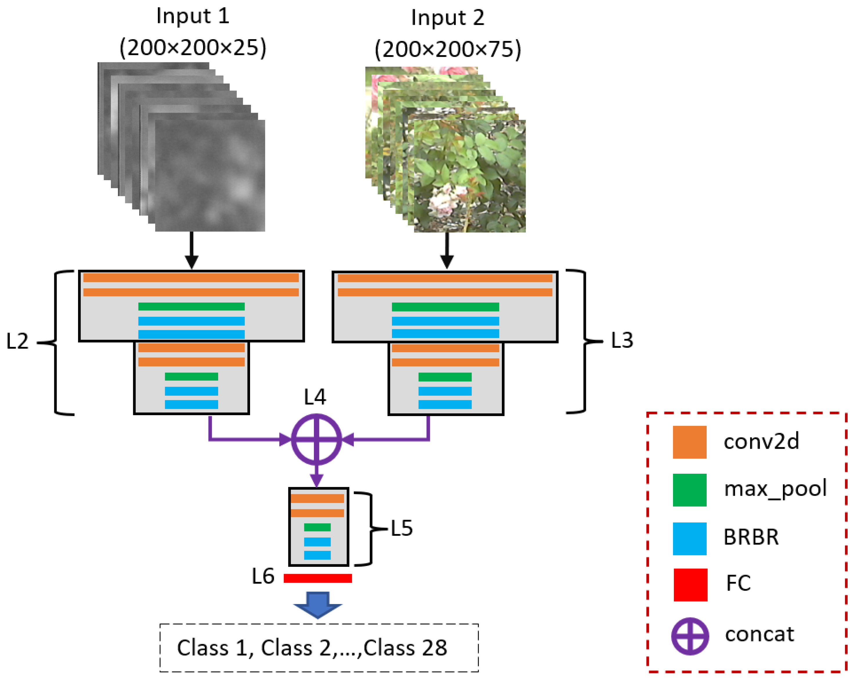
The structure of the proposed PlantMC network is provided in

Table 8. Description of the proposed PlantMC.

Layer#	Times	Layer Type	Filter#	Parameter#		Layer Connection
1	1	input layer_1 & 2	0	0	0	input
2	2	group_1	64/128	1,735,872	1,749,696	input layer_1
3	2	group_2	64/128	1,737,024	1,778,496	input layer_2
4	1	concat	0	0	0	group_1 & group_2
5	1	group_3	128	1,623,808	1,623,808	concat
6	1	FC (softmax)	class#	229,404	14,364	group_3
Total number of trainable parameters: 5,326,108/5,166,364

and Figure 5. The dimensions of the input and output images of the PlantMC network were 200 × 200 × X and 28 × 1, respectively, where X represents the number of channels and is 25 for thermal images and 75 for visible-light images, respectively. The configuration of the group used in Table 8 is identical to that of the discriminator network group shown in Table 5, with the exception of the stride size of the second conv2d being (2 × 2). The input layers (input layer_1 and 2), concatenate layer (concat) and activation layer (softmax) were used to describe the PlantMC network, as provided in Table 8, in contrast to Table 2 and Table 3. The output of the FC layer (class#) is 28. The parameter# column in Table 8 presents the two types of parameter numbers in distinct formats and compares them. For example, the parameter number obtained using the thermal and visible images with dimensions of 600 × 600 × 1 and 600 × 600 × 3, respectively, produced by PlantSR, is provided in non-italic format. However, the parameter number when the preprocessed thermal and visible-light images with dimensions of 200 × 200 × 25 and 200 × 200 × 75, respectively, is shown in italic format for comparison. As shown in Table 8, the number of parameters was lower by 159,744 when using images obtained using preprocessing. The remaining values in Table 8 were consistent with the descriptions in Section 3.3.

3.5. Details of Database and Experimental Setup

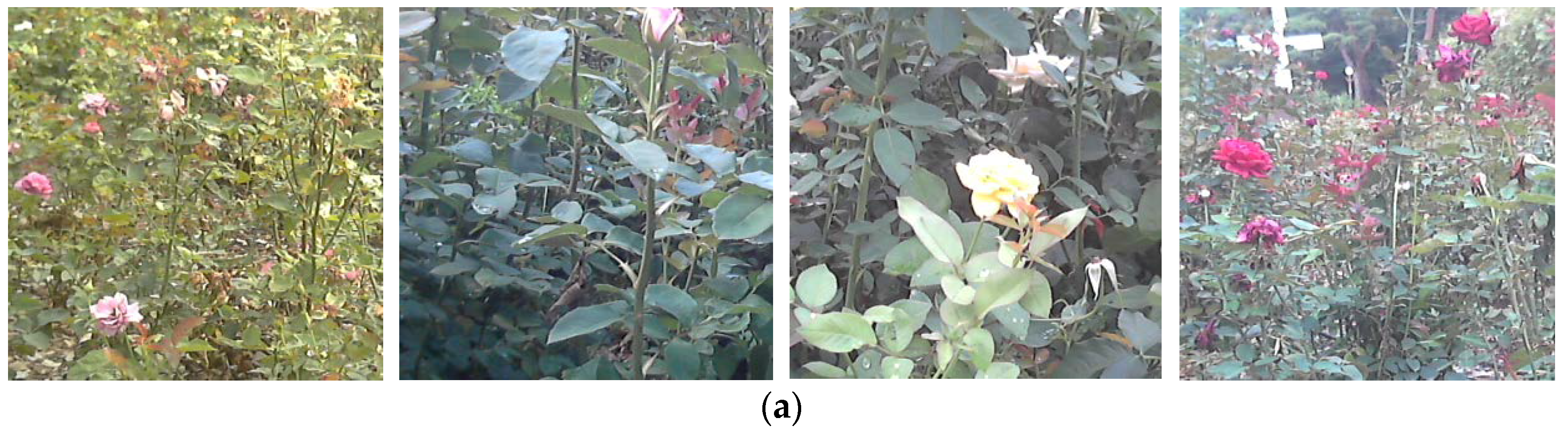
We focused on using both thermal and visible-light images to increase the accuracy of plant classification in this study. However, the existing open datasets, such as PlantVillage [7] and PlantDoc [8] or the others, do not provide thermal images. Therefore, we did not use the datasets in our experiments. Therefore, in this study, the experiments were conducted using the TherVisDb [18] dataset comprising images of various roses and rose leaves. The dataset was obtained in July 2022. The details of the dataset are described in three different tables. In detail,

Table 9. Description of classes and dataset split.

Class Index	Class Names	Image#	Thermal Image#	Visible-Light Image#	Set 1	Set 2	Set 3	Validation Set
1	Alexandra	240	120	120	72	72	72	24
2	Belvedere	96	48	48	28	28	28	12
3	Blue river	272	136	136	82	82	82	26
4	Charm of paris	272	136	136	82	82	82	26
5	Cleopatra	304	152	152	88	88	88	40
6	Cocktail	224	112	112	70	70	70	14
7	Duftrausch	352	176	176	104	104	104	40
8	Echinacea sunset	128	64	64	38	38	38	14
9	Eleanor	288	144	144	88	88	88	24
10	Elvis	448	224	224	134	134	134	46
11	Fellowship	416	208	208	124	124	124	44
12	Goldeise	288	144	144	86	86	86	30
13	Goldfassade	368	184	184	112	112	112	32
14	Grand classe	528	264	264	158	158	158	54
15	Just joey	144	72	72	42	42	42	18
16	Kerria japonica	208	104	104	62	62	62	22
17	Margaret	224	112	112	66	66	66	26
18	Oklahoma	624	312	312	186	186	186	66
19	Pink perfume	240	120	120	72	72	72	24
20	Queen elizabeth	240	120	120	72	72	72	24
21	Rose gaujard	624	312	312	186	186	186	66
22	Rosenau	608	304	304	182	182	182	62
23	Roseraie du chatelet	704	352	352	214	214	214	62
24	Spiraea salicifolia l	128	64	64	38	38	38	14
25	Stella de oro	96	48	48	28	28	28	12
26	Twist	576	288	288	172	172	172	60
27	Ulrich brunner fils	240	120	120	72	72	72	24
28	White symphonie	560	280	280	168	168	168	56
Total		9440	4720	4720	2826	2826	2826	962

describes the names of flowers and class indices; the number of images of each class and three subsets for the 3-fold cross-validation; the number of images in the validation set; the number of thermal and visible-light images, separately; and the total number of images in the dataset. In the table, the ‘Image#’ column represents the sum of numbers of thermal and visible-light images. The ‘Sets 1-3’ column indicates the dataset split for 3-fold cross-validation.

Table 10. Weather information for the surrounding environment at the time of image acquisition.

Types of Weather Measurement	Numerical Values with Units
Humidity	91%
Temperature	30 °C
Wind speed	3 m/s
Fine dust	24 μg/m3
Ultra-fine dust	22 μg/m3
UV index	8

describes the weather information of the day when we collected our dataset, including humidity, temperature, wind speed, fine dust, ultra-fine dust and UV index. Moreover,

Table 11. Other relevant information in the dataset.

Lists		Thermal Image	Visible Light Image	Units
Before augmentation	Image size	640 × 512 × 1	640 × 512 × 3	pixel
	Depth	14	24	bit
	Class number	28	28	-
	Image extension	bmp	bmp	-
	Camera sensor	Flir Tau® 2 [19]	Logitech C270 [20]	-
After augmentation	Image size	300 × 300 × 1	300 × 300 × 3	pixel
	Depth	8	24	bit
	Image extension	png	png	-

describes other information, such as image dimension, depth and extension, before and after augmentation. Moreover, the number of total classes and information of camera sensors were described. In addition, examples of thermal images and corresponding visible-light images in the dataset are presented in Figure 6.

In the “Before augmentation” part in Table 11, a single image included many plants; therefore, such images were cropped into images with a size of 300 × 300 to increase the number of images detailed in the “After augmentation” part in Table 11. The number of images produced as such for each class in the dataset is provided in Table 9. In the training phase, each training set was expanded using augmentation methods (rotating three times by 90° and flipping horizontally). In addition, down-sizing of images from dimensions of 300 × 300 to 200 × 200 was performed to conduct SRR. The computer hardware and software used in this study are described in

Table 12. Description of hardware and software of desktop computer.

Hardware		Software
		Library (Version)
Processor	Intel(R) Core(TM) i7-6700 [email protected] GHz (8 CPUs)	OpenCV [21] (4.3.0), Python [22] (3.5.4), Keras API [23] (2.1.6-tf), TensorFlow [24] (1.9.0)
Main memory	32 GB RAM
GPU	Nvidia GeForce GTX TITAN X (12 GB)

.

4. Experimental Results

This section is divided into four parts: training setup, testing, experimental comparison and processing time. In Section 4.1, the setup of the training phase, characterized by, for example, the hyperparameters and training loss, is described. In Section 4.2, the results obtained from the training phase are presented. Thereafter, the experimental results produced by the existing and proposed methods are compared in Section 4.3. Finally, the processing time of the proposed method is measured in Section 4.4.

4.1. Training Setup

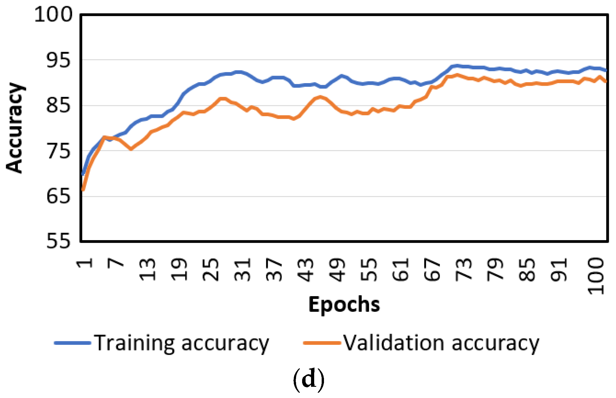
The training setup of the proposed methods is presented in

Table 13. Search spaces and selected values of hyperparameters for the proposed methods.

Parameters	PlantSR		PlantMC
	Search Space	Selected Value	Search Space	Selected Value
Learning rate	[0.00001, 0.0001, 0.001]	0.0001	[0.00001, 0.0001, 0.001]	0.0001
Epochs	[1~100]	92	[1~100]	74
Batch size	[1, 8, 16]	8	[1, 8, 16]	8
Optimizer	Adam [25]	Adam	Adam	Adam
Loss	binary cross-entropy [26]	binary cross-entropy	categorical cross-entropy [27]	categorical cross-entropy

. The training loss and validation accuracy curves of PlantSR and PlantMC are shown in Figure 7. Figure 7a,b show the training and validation loss curves of the PlantSR per epoch. Figure 7c,d show the loss and accuracy curves of the PlantMC per epoch. As is evident, the network developed in this study was sufficiently trained without being overfitted by the training data. In addition, Table 13 presents search spaces and selected values of the hyperparameters for the network.

4.2. Testing

The testing results are presented in this section. To measure the accuracy of PlantSR, Equation (1) for peak signal-to-noise ratio (PSNR) [28] and Equation (2) for structural similarity index measure (SSIM) [29] were used. Further, Equations (3)–(6) were employed to calculate the accuracy of PlantMC.

$$\mathrm{PSNR}=10lo{g}_{10}\left(\frac{{255}^2}{\frac{{\left(\sqrt{{{\displaystyle \sum }}_{\mathrm{j}=1}^{\mathrm{M}}{{\displaystyle \sum }}_{\mathrm{i}=1}^{\mathrm{N}}{\left(\mathrm{X}\left(\mathrm{i},\mathrm{j}\right)-\mathrm{Y}\left(\mathrm{i},\mathrm{j}\right)\right)}^2}\right)}^2}{\mathrm{MN}}}\right)$$

(1)

where X, Y, M and N represent original image, restored image, image width and image height, respectively.

$$\mathrm{SSIM}=\frac{\left(2{\mathsf{\mu }}_{\mathrm{Y}}{\mathsf{\mu }}_{\mathrm{X}}+\mathrm{C}1\right)\left(2{\mathsf{\sigma }}_{\mathrm{XY}}+\mathrm{C}2\right)}{\left({\mathsf{\mu }}_{\mathrm{Y}}{}^2+{\mathsf{\mu }}_{\mathrm{X}}{}^2+\mathrm{C}1\right)\left({\mathsf{\sigma }}_{\mathrm{Y}}{}^2+{\mathsf{\sigma }}_{\mathrm{X}}{}^2+\mathrm{C}2\right)}$$

(2)

where ${\mathsf{\mu }}_{\mathrm{X}}$ and ${\mathsf{\sigma }}_{\mathrm{X}}$ represent the mean and standard deviation of the pixel values of a ground-truth image, respectively, ${\mathsf{\mu }}_{\mathrm{Y}}$ and ${\mathsf{\sigma }}_{\mathrm{Y}}$ represent the mean and standard deviation of the pixel values of the restored image, respectively, and ${\mathsf{\sigma }}_{\mathrm{XY}}$ is the covariance in the two images. Moreover, C1 and C2 are positive constants.

TPR = (#TP)/(#TP + #FN)

(3)

PPV = (#TP)/(#TP + #FP)

(4)

ACC = (#TP + #TN)/(#TP + #TN + #FP + #FN)

(5)

where the numbers of true positive (#TP), false positive (#FP), false negative (#FN) and true negative (#TN) were provided to calculate true-positive rate (TPR), positive predictive values (PPV), accuracy (ACC) [30] and F1-score [31].

F1-score = 2·(PPV·TPR)/(PPV + TPR)

(6)

Table 14. Comparison of accuracies obtained in different folds using PlantSR + PlantMC.

Methods	PPV	TPR	F1-Score	ACC
Fold-1	91.25	91.46	91.46	99.94
Fold-2	90.26	89.86	89.61	98.82
Fold-3	90.08	89.73	89.40	98.90
Average	90.53	90.35	90.16	99.22

,

Table 15. Comparison of accuracies obtained by using classification methods with and without RBRB.

Methods	PPV	TPR	F1-Score	ACC
PlantMC without RBRB	89.47	90.11	89.75	98.21
PlantMC with RBRB	90.53	90.35	90.16	99.22

and

Table 16. Comparison of accuracies obtained using classification methods using images with different sizes and channels.

Methods	PPV	TPR	F1-Score	ACC
PlantMC using 600 × 600 × 1 (3)	90.4	90.45	90.1	99.21
PlantMC using 200 × 200 × 25 (75)	90.53	90.35	90.16	99.22

present the results of performing classification using the image reconstructed with PlantSR as the input for PlantMC. Table 14 presents and compares each of the results of 3-fold cross-validation. As shown in Table 14, accuracies obtained in the three folds are almost similar to each other and fold-1 showed the highest accuracy, whereas fold-3 showed the lowest. Table 15 compares the results from the method using RBRB (two residual blocks followed by an addition operation, as shown in Table 6) and those from the method not using RBRB (two residual blocks not followed by an addition operation). Evidently, the accuracy results produced using RBRB were greater. Therefore, we used the RBRB in further experiments in this study; moreover, we propose the RBRB in this study for the increased accuracy of the plant image classification. The results using images modified through preprocessing, of 200 × 200 × 25 (75) dimensions, those using images without preprocessing, of 600 × 600 × 1 (3) dimensions, are provided for comparison in Table 16. Although preprocessing did not improve the accuracy by a significant amount, it decreased the number of parameters and reduced the memory size, as demonstrated in Table 8. In addition, it reduced the processing time, as is evident in Section 4.4.

Table 17. Detailed accuracy of each class by the proposed PlantSR and PlantMC with and without PlantSR.

#	Class Names	PlantSR (Th)		PlantSR (V)		PlantMC				PlantSR + PlantMC
		PSNR	SSIM	PSNR	SSIM	PPV	TPR	F1-Score	ACC	PPV	TPR	F1-Score	ACC
1	Alexandra	26.87	0.87	27.41	0.88	91.48	99.39	95.27	99.43	92.32	99.52	95.79	100
2	Belvedere	26.59	0.89	28.18	0.88	99.68	82.73	90.42	98.95	100	83.69	91.19	99.75
3	Blue river	27.27	0.86	27.6	0.95	92.61	83.19	87.65	99.24	93.23	84.17	88.47	100
4	Charm of paris	27	0.84	27.46	0.87	81.52	85	83.22	98.66	81.74	85.9	83.77	99.63
5	Cleopatra	27.3	0.92	27.67	0.89	57.59	94.7	71.62	98.37	58.43	95.05	72.37	98.55
6	Cocktail	27.12	0.93	27.57	0.95	90.31	90.66	90.49	99.2	91.08	91.54	91.31	99.76
7	Duftrausch	27.36	0.93	27.8	0.93	93.58	96.76	95.14	99.02	94.15	97.17	95.64	99.19
8	Echinacea sunset	27.42	0.9	28.14	0.85	91.94	91.63	91.79	99.22	92.43	91.95	92.19	99.54
9	Eleanor	27.4	0.91	27.9	0.87	99.18	99.57	99.38	99.99	99.63	100	99.95	100
10	Elvis	27.12	0.9	27.93	0.92	92.9	85.39	88.99	98.12	93.66	86.36	89.86	98.98
11	Fellowship	26.88	0.88	28.02	0.86	89.51	85.98	87.71	98.51	89.72	85.98	87.81	99.47
12	Goldeise	27.41	0.92	27.68	0.92	92.75	81.46	86.74	98.5	93.44	82.16	87.44	99.35
13	Goldfassade	27.08	0.91	27.58	0.88	91.51	86.96	89.18	99.16	91.63	87.56	89.55	99.9
14	Grand classe	27.24	0.85	28.13	0.89	81.11	85.5	83.24	97.44	81.4	85.54	83.42	97.89
15	Just joey	27.4	0.89	27.84	0.92	86.45	76.46	81.14	98.62	87.25	76.96	81.78	98.83
16	Kerria japonica	27.11	0.89	27.38	0.94	99.89	99.37	99.63	99.22	100	100	100	99.26
17	Margaret	27.18	0.91	27.91	0.93	82.59	86.1	84.31	98.87	83.47	86.62	85.02	99.45
18	Oklahoma	26.47	0.86	27.97	0.93	91.89	86.19	88.95	98.5	92.40	87.06	89.65	98.68
19	Pink perfume	27.37	0.87	27.48	0.88	83.17	90.54	86.7	98.46	83.37	91.27	87.14	98.54
20	Queen elizabeth	27.05	0.92	28.15	0.91	95.81	95.31	95.56	98.97	96.78	95.63	96.2	99.65
21	Rose gaujard	26.66	0.87	27.8	0.91	91.88	84.31	87.93	98.06	92.84	85.25	88.88	98.4
22	Rosenau	26.73	0.88	27.69	0.93	99.46	90.05	94.52	98.42	99.8	90.95	95.17	98.47
23	Roseraie du chatelet	26.89	0.85	28.2	0.94	82.28	94.23	87.85	97.95	82.75	94.33	88.16	98.06
24	Spiraea salicifolia l	27.44	0.89	28.21	0.95	99.73	99.38	99.55	99.47	99.84	99.75	99.8	100
25	Stella de oro	27.09	0.84	27.78	0.89	99.42	90.33	94.66	98.93	99.96	91.12	95.34	99.4
26	Twist	26.51	0.84	28.05	0.88	90.51	94.44	92.43	98.28	91.45	94.51	92.96	98.93
27	Ulrich brunner fils	26.67	0.84	27.64	0.94	78.88	86.04	82.31	98.77	79.35	86.83	82.92	99.13
28	White symphonie	27.29	0.88	28.33	0.9	92.46	92.17	92.31	98.34	92.77	92.94	92.85	99.23
	Average	27.07	0.88	27.84	0.91	90	89.78	89.6	98.74	90.53	90.35	90.16	99.22

presents the results of using thermal images as the input to PlantSR (PlantSR (Th)) and results of using visible-light images as the input to PlantSR (PlantSR (V)). In addition, PlantMC results, with and without PlantSR, are compared. Further, the accuracy of each proposed method is provided with class-based comparisons. As demonstrated, the accuracy of classification with SRR (PlantSR + PlantMC) was higher than that of classification without SRR (PlantMC). Moreover, Spiraea salicifolia l and White symphonie showed the highest PSNRs of 27.44 and 28.33 in PlantSR (Th) and PlantSR (V), respectively, whereas Oklahoma and Kerria japonica showed the lowest PSNRS of 26.47 and 27.38 in PlantSR (Th) and PlantSR (V), respectively. Moreover, Kerria japonica showed the highest F1-scores of 99.63 and 100 in both PlantMC and PlantSR+PlantMC, respectively, whereas Cleopatra showed the lowest F1-scores of 71.62 and 72.37 in both PlantMC and PlantSR + PlantMC, respectively.

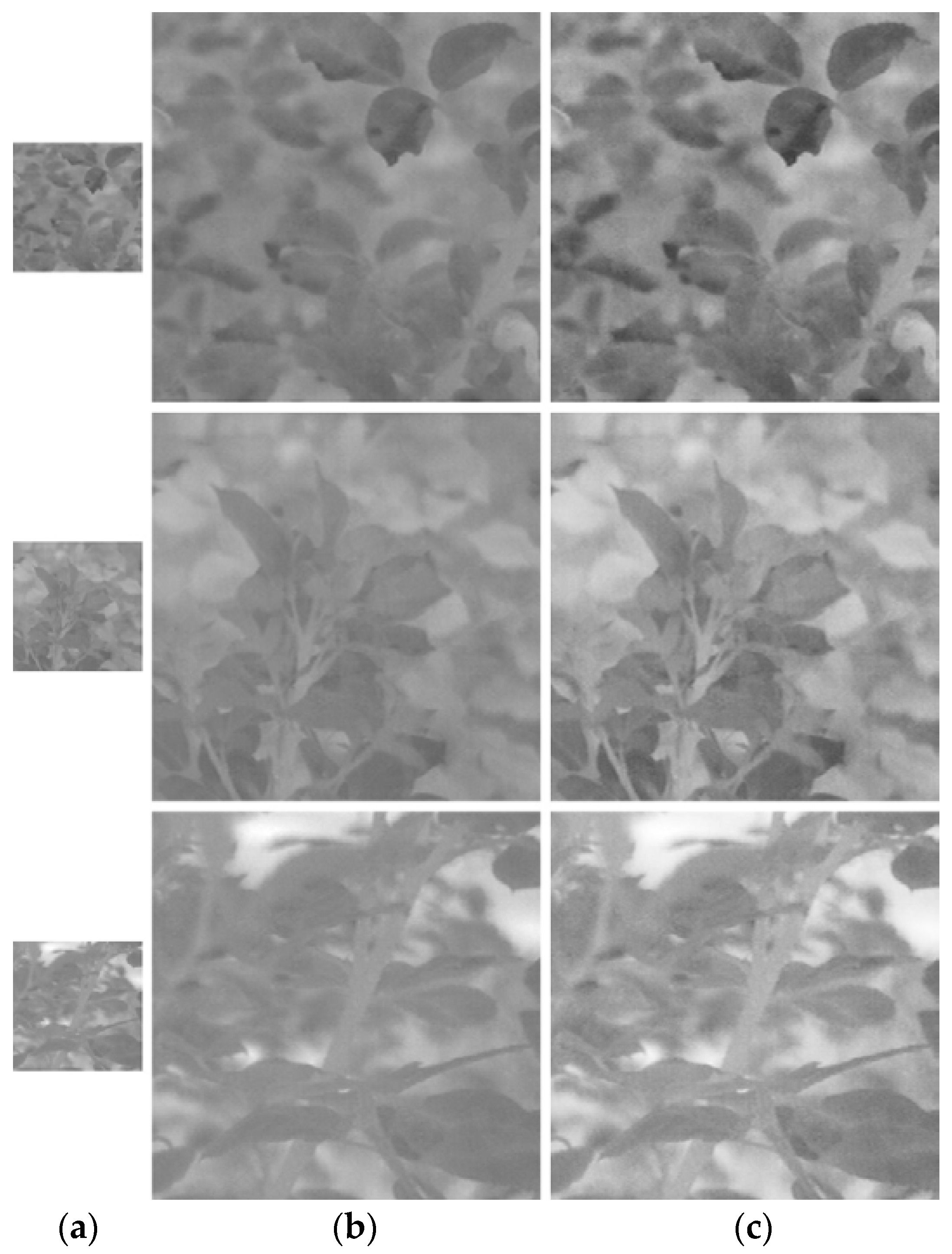
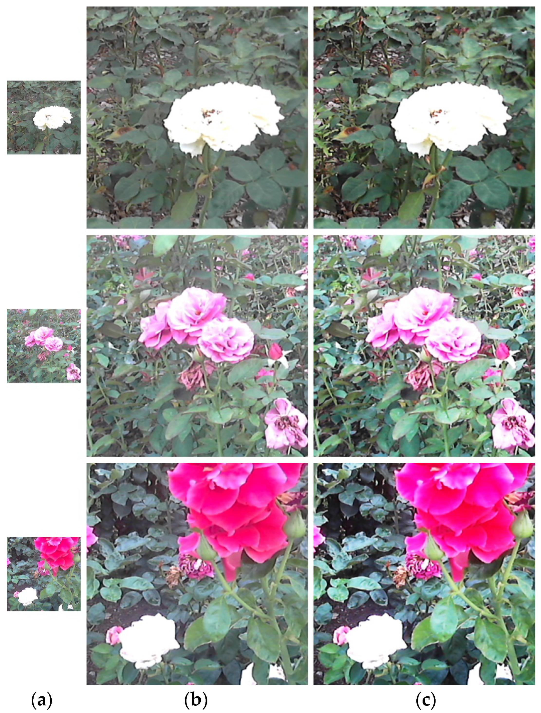
Figure 8 and Figure 9 show that the images produced using the proposed method exhibited sharper contrast than those produced using the bicubic method, which means that the proposed method can generate plant images with higher contrast than the conventional bicubic method. As shown in

Table 18. Comparison of accuracies by bicubic and the proposed PlantSR, and PlantMC with bicubic and PlantSR.

Images	SRR		PlantMC				SRR + PlantMC
	PSNR	SSIM	PPV	TPR	F1-Score	ACC	PPV	TPR	F1-Score	ACC
Original images	-	-	90	89.78	89.6	98.74	-	-	-	-
Bicubic (Th)	27	0.86	-	-	-	-	90.05	89.97	89.87	98.9
Bicubic (V)	27.7	0.89	-	-	-	-
PlantSR (Th)	27.07	0.88	-	-	-	-	90.53	90.35	90.16	99.22
PlantSR (V)	27.84	0.91	-	-	-	-

, the accuracy and classification efficiency results obtained using PlantSR were higher than those obtained using bicubic. Table 18 also demonstrates that classification performance using bicubic and PlantSR-reconstructed images exhibited higher efficiency compared to the results using the original image. This analysis supports the positive influence of SRR on the classification performance. Moreover, it means that the proposed SRR method increases the performance of the classification method.

4.3. Comparisons with the Existing Methods

In this section, the proposed methods are compared to the state-of-the-art methods experimentally. As this study is the first to perform SRR and classification using plant thermal and visible-light images, there are no similar existing methods for a fair comparison, as supported by Table 1. Therefore, the existing methods of SRR and classification using plant visible-light images [15,16] were used for comparative analysis. The existing plant image SRR and classification methods [15,16] were compared to the proposed methods (PlantSR, PlantMC and PlantSR + PlantMC), as presented in

Table 19. Comparison of accuracies obtained by using SRR methods.

Methods	PSNR	SSIM
Bicubic	27.7	0.89
Method-1 [15]	27.71	0.88
Method-2 [16]	27.73	0.89
PlantMC	27.84	0.91

,

Table 20. Comparison of accuracies obtained by using classification methods without SRR.

Methods	PPV	TPR	F1-Score	ACC
Method-1 [15]	88.13	89.49	88.71	98.21
Method-2 [16]	88.93	89.07	89.03	98.66
PlantMC	90	89.78	89.6	98.74

and

Table 21. Comparison of accuracies obtained by using classification methods with SRR.

Methods	PPV	TPR	F1-Score	ACC
Method-1 with SRR [15]	89.39	90.12	89.98	98.79
Method-2 with SRR [16]	89.75	90.21	90.05	99.1
PlantSR + PlantMC	90.53	90.35	90.16	99.22

. When the experimental comparison was conducted, training was executed on the TherVisDb database for the existing methods [15,16]. The detailed explanations on the SRR and CNN configuration used by the existing method-1 [15] can be found in [15] and [33], respectively. Further, the detailed description of the SRR and CNN configuration used by the existing method-2 can be found in [16,34]. The previous study [16] used a modified VGG-Net proposed in study [34] as a classification network. The experimental results for plant image SRR and plant image classification were compared in Section 4.3.1 and Section 4.3.2, respectively.

4.3.1. Comparisons with Plant Image SRR Methods

In this section, the existing plant image-based SRR methods are used for comparative analysis. As is evident in Table 1, there is no existing study on plant thermal image-based SRR method; thus, the plant visible-light image was used for comparison. The SRR methods employed in Method-1 and Method-2 were used in comparison in Table 19, and the accuracy results obtained from the proposed method were the highest. Moreover, the proposed method showed the highest accuracy, whereas the Bicubic showed the lowest accuracy. In addition, the SRR methods showed very little difference in accuracy. Figure 10 presents a graphical comparison of the SRR methods.

4.3.2. Comparisons with Plant Image Classification Methods

In this section, the existing plant image-based SRR and classification methods were used for comparative analysis. While only visible-light images were used by Method-1 and Method-2, both thermal and visible-light images were used by the proposed method. Under both experimental conditions, the proposed method produced the highest accurate results, as is evident in Table 20 and Table 21. These results confirmed that the use of thermal and visible-light images simultaneously, as in the proposed method, was efficient. In addition, Table 18, Table 20 and Table 21 demonstrate that classification results using SRR are more accurate, thereby confirming that SRR is effective in plant classification. Moreover, in all cases, the proposed method showed higher accuracies than the other methods.

In Table 19, Table 20 and Table 21, the outperformance of the proposed method is not significant. Because the previous networks (method-1 [15] and method-2 [16]) used larger numbers of parameters, layers and additional networks for super-resolution reconstruction (SRR), the proposed method could not outperform their results significantly. For example, a classification network of method-1 [15] has over 62 million parameters, whereas our classification network has only 5 million parameters. Moreover, they used a super-resolution convolutional neural network (SRCNN) for SRR, which was pretrained with the ImageNet database, including huge numbers of images. However, the SRCNN was not used in our method, which makes it difficult to achieve a significant result compared to the previous method [15]. The classification networks of method-2 [16] and the proposed method are similar; however, their SRR network has a total of 115 convolution layers, whereas our SRR network has only 12 convolution layers. Accordingly, it is difficult to achieve a significant result compared to the previous method [16].

4.4. Processing Time of the Methods

The processing time of the proposed PlantSR and PlantMC in the testing phase is shown in

Table 22. Processing time of the methods per image (unit: ms).

Database	Processing Time
PlantSR using thermal image	68.45
PlantSR using visible-light image	62.75
PlantMC using 600 × 600 × 1 (3)	58.24
PlantMC using 200 × 200 × 25 (75)	46.12
PlantSRs + PlantMC using 200 × 200 × 25 (75)	177.32

. Table 22 presents the frame rates of PlantSR methods using thermal and visible-light images, which were 14.6 and 15.93 frames per second (fps), respectively. The frame rate of the PlantSRs + PlantMC method was 5.63 fps. In addition, the frame rate when PlantSR-produced thermal and visible-light images with dimensions of 600 × 600 × 1 and 600 × 600 × 3, respectively, were used was 17.17 fps. As demonstrated, the frame rate obtained according to the method proposed in Figure 2 and Figure 3, which involves using preprocessed thermal and visible-light images with dimensions of 200 × 200 × 25 and 200 × 200 × 75, was 21.68 fps.

5. Discussion

In this study, SRR and classification using plant thermal and visible-light images were examined. Using the two types of images as separate inputs for the proposed method (PlantSR) produced bigger images with sharper contrast, as demonstrated in Figure 8 and Figure 9. Further, the proposed method (PlantMC) exhibited higher improved performance when PlantSR was employed to produce and integrate the two types of images, as shown in Table 17. As demonstrated by Table 20 and Table 21, the proposed method delivered higher performance than the methods introduced by the existing studies. In addition, the method of using the preprocessed thermal and visible-light images with dimensions of 200 × 200 × 25 (75) was faster than the method using the PlantSR-produced images with dimensions of 600 × 600 × 1 (3). The measures of accuracy of the two methods did not differ significantly, as shown in Table 16. Furthermore, the results of the method with RBRB (two residual blocks followed by an addition operation, as shown in Table 6) that is newly developed in this study were compared to those of the method without RBRB (two residual blocks not followed by an addition operation) in Table 15. Evidently, the accuracy results with the application of RBRB were higher.

Figure 11 and Figure 12 show error cases by the proposed method, PlantMC. The classification error of PlantMC was influenced by the image that is wrongly reconstructed by PlantSR. As is evident, when the image was too bright or too dark, even brighter or darker images were produced. In contrast, the images produced using the bicubic appeared clearer than those produced by PlantSR.

6. Conclusions

In this study, the SRR and plant classification methods based on thermal and visible-light images were proposed and tested. The TherVisDb dataset was utilized in various experiments in the study. The dataset contained various images of roses and rose leaves. Based on the plant image classification experiment using TherVisDb, the accuracy of the proposed method appeared higher than that of existing methods, with an accuracy of 99.22% and F1-score of 90.16%. In addition, the results of the plant image SRR experiment using TherVisDb revealed that the proposed method was more accurate than the existing method, as is evident from the PSNR of 27.84 and SSIM of 0.91.

The experimental results provided in Table 18 confirmed that the accuracy of classification increased when the images were expanded using PlantSR. As explained for the preprocessing in Section 3.2, by reducing the dimensions of PlantSR-produced images and increasing the number of channels in exchange, the processing time, number of parameters and memory size of PlantMC were decreased, as is evident in Table 8 and Table 22.

Further, Table 15 indicates that the use of RBRB newly developed in this study was confirmed to produce higher accuracy than the method using the basic residual block.

In future work, various deep learning methods will be considered to reduce the SRR and classification errors exhibited in Figure 11 and Figure 12. Furthermore, the SRR and classification process to increase the accuracy of the proposed method will be explored.

References

- PlantSR & PlantMC. Available online: https://github.com/ganav/PlantSR-PlantMC (accessed on 22 November 2022).
- Abawatew, G.Y.; Belay, S.; Gedamu, K.; Assefa, M.; Ayalew, M.; Oluwasanmi, A.; Qin, Z. Attention augmented residual network for tomato disease detection and classification. Turk. J. Electr. Eng. Comput. Sci. 2021, 29, 2869–2885. [Google Scholar]
- Chakraborty, A.; Kumer, D.; Deeba, K. Plant leaf disease recognition using fastai image classification. In Proceedings of the 2021 5th International Conference on Computing Methodologies and Communication (ICCMC), Erode, India, 8–10 April 2021; pp. 1624–1630. [Google Scholar] [CrossRef]
- Ashwinkumar, S.; Rajagopal, S.; Manimaran, V.; Jegajothi, B. Automated plant leaf disease detection and classification using optimal MobileNet based convolutional neural networks. Mater. Today Proc. 2022, 51, 480–487. [Google Scholar] [CrossRef]
- Chompookham, T.; Surinta, O. Ensemble methods with deep convolutional neural networks for plant leaf recognition. ICIC Express Lett. 2021, 15, 553–565. [Google Scholar]
- Wang, D.; Wang, J.; Li, W.; Guan, P. T-CNN: Trilinear convolutional neural networks model for visual detection of plant diseases. Comput. Electron. Agric. 2021, 190, 106468. [Google Scholar] [CrossRef]
- PlantVillage Dataset. Available online: https://www.kaggle.com/datasets/emmarex/plantdisease (accessed on 16 September 2022).
- Singh, D.; Jain, N.; Jain, P.; Kayal, P.; Kumawat, S.; Batra, N. PlantDoc: A dataset for visual plant disease detection. In Proceedings of the 7th ACM IKDD CoDS and 25th COMAD, Hyderabad, India, 5–7 January 2020; pp. 249–253. [Google Scholar] [CrossRef] [Green Version]
- Batchuluun, G.; Nam, S.H.; Park, K.R. Deep learning-based plant-image classification using a small training dataset. Mathematics 2022, 10, 3091. [Google Scholar] [CrossRef]
- Batchuluun, G.; Nam, S.H.; Park, K.R. Deep learning-based plant classification and crop disease classification by thermal camera. J. King Saud Univ. Comput. Inf. Sci. 2022, 1319–1578, in press. [Google Scholar] [CrossRef]
- Raza, S.E.; Prince, G.; Clarkson, J.P.; Rajpoot, N.M. Automatic detection of diseased tomato plants using thermal and stereo visible light images. PLoS ONE 2015, 10, e0123262. [Google Scholar] [CrossRef] [PubMed]
- Analysis of Variance. Available online: https://en.wikipedia.org/wiki/Analysis_of_variance (accessed on 16 September 2022).
- Tong, S.; Koller, D. Support vector machine active learning with applications to text classification. J. Mach. Learn. Res. 2002, 2, 45–66. [Google Scholar] [CrossRef]
- Batchuluun, G.; Nam, S.H.; Park, K.R. Deep learning-based plant classification using nonaligned thermal and visible light images. Mathematics 2022, 10, 4053. [Google Scholar] [CrossRef]
- Yamamoto, K.; Togami, T.; Yamaguchi, N. Super-Resolution of Plant Disease Images for the Acceleration of Image-based Phenotyping and Vigor Diagnosis in Agriculture. Sensors 2017, 17, 2557. [Google Scholar] [CrossRef] [PubMed]
- Cap, Q.H.; Tani, H.; Uga, H.; Kagiwada, S.; Iyatomi, H. Super-resolution for practical automated plant disease diagnosis system. arXiv 2019, arXiv:1911.11341v1. [Google Scholar]
- Goodfellow, I.J.; Pouget-Abadie, J.; Mirza, M.; Xu, B.; Warde-Farley, D.; Ozair, S.; Courville, A.; Bengio, Y. Generative adversarial networks. arXiv 2014, arXiv:1406.2661v1. [Google Scholar] [CrossRef]
- TherVisDb. Available online: https://github.com/ganav/PlantCR-TherVisDb/tree/main (accessed on 28 September 2022).
- Flir Tau® 2. Available online: https://www.flir.com/products/tau-2/ (accessed on 31 October 2022).
- Logitech C270 HD Web-Camera. Available online: https://www.logitech.com/en-us/products/webcams/c270-hd-webcam.960-000694.html (accessed on 6 September 2022).
- OpenCV. Available online: http://opencv.org/ (accessed on 16 September 2022).
- Python. Available online: https://www.python.org/ (accessed on 16 September 2022).
- Chollet, F. Keras. California, U.S. Available online: https://keras.io/ (accessed on 16 September 2022).
- TensorFlow. Available online: https://www.tensorflow.org/ (accessed on 26 October 2022).
- Kingma, D.P.; Ba, J.B. ADAM: A method for stochastic optimization. In Proceedings of the 3rd International Conference on Learning Representations, San Diego, CA, USA, 7–9 May 2015; pp. 1–15. [Google Scholar]
- Cross-Entropy Loss. Available online: https://en.wikipedia.org/wiki/Cross_entropy (accessed on 26 October 2022).
- Categorical Cross-Entropy Loss. Available online: https://peltarion.com/knowledge-center/documentation/modeling-view/build-an-ai-model/loss-functions/categorical-crossentropy (accessed on 16 September 2022).
- Wang, Z.; Bovik, A.C.; Sheikh, H.R.; Simoncelli, E.P. Image quality assessment: From error visibility to structural similarity. IEEE Trans. Image Process. 2004, 13, 600–612. [Google Scholar] [CrossRef] [Green Version]
- Huynh-Thu, Q.; Ghanbari, M. Scope of validity of psnr in image/video quality assessment. Electron. Lett. 2008, 44, 800–801. [Google Scholar] [CrossRef]
- Powers, D.M.W. Evaluation: From precision, recall and f-measure to roc, informedness, markedness & correlation. Mach. Learn. Technol. 2011, 2, 37–63. [Google Scholar]
- Derczynski, L. Complementarity, F-score, and NLP evaluation. In Proceedings of the Tenth International Conference on Language Resources and Evaluation 2016, Portorož, Slovenia, 23–28 May 2016; European Language Resources Association: Paris, France, 2016; pp. 261–266. [Google Scholar]
- Keys, R. Cubic convolution interpolation for digital image processing. IEEE Trans. Acoust. Speech Signal Process. 1981, 29, 1153–1160. [Google Scholar] [CrossRef] [Green Version]
- Krizhevsky, A.; Sutskever, I.; Hinton, G.E. ImageNet classification with deep convolutional neural networks. Adv. Neural Inf. Process. Syst. 2012, 25, 1097–1105. [Google Scholar] [CrossRef] [Green Version]
- Tani, H.; Kotani, R.; Kagiwada, S.; Uga, H.; Iyatomi, H. Diagnosis of multiple cucumber infections with convolutional neural networks. In Proceedings of the 2018 IEEE Applied Imagery Pattern Recognition Workshop (AIPR), Washington, DC, USA, 9–11 October 2018; pp. 1–4. [Google Scholar] [CrossRef]
Figure 1.
Overview of the proposed method for plant image SRR and classification.
Figure 2.
Example of preprocessing on thermal image.
Figure 3.
Preprocessing of visible-light image.
Figure 4.
Detailed structure of PlantSR.
Figure 5.
Detailed structure of PlantMC.
Figure 6.
Example images of TherVisDb. From left to right: images of blue river, charm of Paris, Cleopatra and cocktail. (a) Visible-light images and (b) corresponding thermal images.
Figure 7.
Loss and accuracy curves of the PlantSR and PlantMC. (a) Training loss curves of PlantSR; (b) validation loss curves of PlantSR; (c) training and validation loss curves of PlantMC; (d) training and validation accuracy curves of PlantMC.
Figure 8.
Example thermal images generated by PlantSR. From top to bottom, images of Rose gaujard, Duftrausch and Elvis. (a) Original image; (b) enlarged image by bicubic [32]; (c) enlarged image by PlantSR.
Figure 9.
Example visible-light images generated by PlantSR. From top to bottom, images of White symphonie, Roseraie du chatelet and Twist. (a) Original image; (b) enlarged image by bicubic; (c) enlarged image by PlantSR.
Figure 10.
Example visible-light images generated by SRR methods. From top to bottom, images of White symphonie, Roseraie du chatelet and Twist. (a) Original image; (b) enlarged image by bicubic; (c) enlarged image by Method-1; (d) enlarged image by Method-2; (e) enlarged image by PlantSR.
Figure 11.
Example of error cases of thermal images generated by PlantSR. From top to bottom, images of Rose gaujard, Duftrausch and Elvis. (a) Original image; (b) enlarged image by bicubic; (c) enlarged image by PlantSR.
Figure 12.
Example of error cases of visible-light images generated by PlantSR. From top to bottom, images of White symphonie, Roseraie du chatelet and Twist. (a) Original image; (b) enlarged image by bicubic; (c) enlarged image by PlantSR.