
Survey of Optimization Algorithms in Modern Neural Networks

1
North-Caucasus Center for Mathematical Research, North-Caucasus Federal University, 355009 Stavropol, Russia
2
Department of Mathematical Modeling, North-Caucasus Federal University, 355009 Stavropol, Russia
*
Author to whom correspondence should be addressed.
Mathematics 2023, 11(11), 2466; https://0-doi-org.brum.beds.ac.uk/10.3390/math11112466
Submission received: 19 April 2023
/
Revised: 19 May 2023
/
Accepted: 25 May 2023
/
Published: 26 May 2023
(This article belongs to the Special Issue Mathematical Foundations of Deep Neural Networks)
Abstract
:The main goal of machine learning is the creation of self-learning algorithms in many areas of human activity. It allows a replacement of a person with artificial intelligence in seeking to expand production. The theory of artificial neural networks, which have already replaced humans in many problems, remains the most well-utilized branch of machine learning. Thus, one must select appropriate neural network architectures, data processing, and advanced applied mathematics tools. A common challenge for these networks is achieving the highest accuracy in a short time. This problem is solved by modifying networks and improving data pre-processing, where accuracy increases along with training time. Bt using optimization methods, one can improve the accuracy without increasing the time. In this review, we consider all existing optimization algorithms that meet in neural networks. We present modifications of optimization algorithms of the first, second, and information-geometric order, which are related to information geometry for Fisher–Rao and Bregman metrics. These optimizers have significantly influenced the development of neural networks through geometric and probabilistic tools. We present applications of all the given optimization algorithms, considering the types of neural networks. After that, we show ways to develop optimization algorithms in further research using modern neural networks. Fractional order, bilevel, and gradient-free optimizers can replace classical gradient-based optimizers. Such approaches are induced in graph, spiking, complex-valued, quantum, and wavelet neural networks. Besides pattern recognition, time series prediction, and object detection, there are many other applications in machine learning: quantum computations, partial differential, and integrodifferential equations, and stochastic processes.
Keywords:
optimization methods; physics-informed neural networks; spiking neural networks; quantum neural networks; graph neural networks; information geometry; quasi-Newton methods; approximation; quantum computations; gradient-free optimization; fractional order optimization; bilevel optimizationMSC:
62B11; 68T07; 68T201. Introduction
The question of increasing the accuracy of neural networks remains relevant. There exist many approaches to solve this problem, including the data augmentation [1], improving the mathematical model of neurons [2], adding the complement neural network [3], and so on. Indeed, all these approaches solve the problem of increasing the accuracy in neural networks, but these approaches are not generalized for all models. Thus, there exist universal methods that improve neural network training. One such is the optimization of the loss function. The main problem in neural networks is a descent to the global minimum. The first attempts to achieve the minimal value were realized using stochastic gradient descent (SGD) [4]. Such a first-order optimizer is still widely used in modern neural networks. Later, SGD was equipped with momentum and Nesterov condition (SGDM Nesterov) [5]. This modification increased the convergence rate with high accuracy in fewer iterations.
According to the structure of SGD, there has been proposals of AdaGrad in [6], RMSProp [7], Adadelta [8], and Adam [9], which allow attaining the minimum of functions that contain local extremes. In the case of the Rastrigin, Rosenbrouck, and Ackley functions from [10], these approaches do not reach the global minimum. This happens by achieving the minimum, considering only gradient directions. Exponential moving averages do not suffice for the minimization of such test functions. The same technique is used in modifications of Adam and SGD. Updating the exponential moving averages, Adam-type algorithms are built to improve the minimization for multi-extreme functions. The advantage of these approaches is that the initialization of biases can be counteracted, resulting in bias-corrected estimates. However, they can minimize the loss function but not always at the global minimum. Therefore, second-order optimization should be applied for higher accuracy attaining.
The main goal of second-order optimization algorithms [11] is to achieve the global minimum in a short time, because they are slower that first-order optimization algorithms. Second-order algorithms consider the convexity (curvature) of objective functions by the Hessian matrix. This approach is called the Newton optimization method [12]. Computations of an inverted Hessian matrix make second-order optimization more complex. In machine learning, Newton optimization is an ineffective tool due to the number of neurons, which can exceed one hundred. However, the approximation of inverted Hessian matrix allows the loss function to be minimized within the required time consumption. Such a technique is called the quasi-Newton optimization method [13]. Quasi-Newton optimization algorithms analyze the loss function from a functional point of view, which allows the local extremes to be avoided and rapid convergence in the global minimum. For the improvement of minimization, we observe the objective function from geometric and probabilistic points of view.
The first attempt to geometrically minimize smooth functions was applied in [14], where authors engaged the properties of Riemannian geometry. Such an optimization used the gradient flow for receiving the global minimum. Later, there was an idea to engage information geometry in [15], which is an intersection of Riemannian geometry and probability theory. Such an approach is divided into two branches, which utilize Fisher–Rao [16] or Bregman [17] metrics. The optimization with Fisher–Rao metrics (Fisher information matrix) is called a natural gradient descent. In the case of utilizing Bregman metrics, one receives the mirror descent. These optimization algorithms have demonstrated abilities in pattern recognition [18] and time series prediction [19]. They mainly find application in physics-informed neural networks [20], which are devoted to solving partial differential and integrodifferential equations.
The main goal of this article is to classify optimization algorithms, identify their properties, and provide minimization techniques for further research. After gradient-based optimization methods, we demonstrate alternative approaches to loss function minimization: gradient-free and bilevel optimization.
All provided optimization algorithms are presented in Figure 1, which indicates the contents covered in this paper.
In Table 1, reviews have provided an incomplete classification of all existing optimization methods, such as first-order (SGD and Adam type), second-order (Newtonian and quasi-Newtonian), information-geometric, fractional, and gradient-free methods. In [21], authors present only SGD, NAG, AdaGrad, AdaDelta, RMSProp, Adam, NAdam, and AMSGrad. These optimizers are well known and do not provide new ideas for further research. In many other articles, fractional optimizers use the well-known Riemann–Liouville, Caputo, and Grunwald–Letnikov derivatives. In the review [22], the author classifies all existing fractional derivatives with the corresponding generalizations: Tarasov, Hadamard, Marchaux, Liouville–Weil, and others. In [23], the researchers introduced first-order, info-geometric, fractional, and gradient-free optimizers. The fractional approach is well described for activation functions in recurrent, convolutional, and complex-valued neural networks. Particle swarm optimization and information-geometric Levenberg–Marquardt algorithm are briefly presented. In this review, we have shown all existing types of optimizers. We have described the most promising approaches in machine learning, namely the natural gradient and mirror descent algorithms, which are well described in [24].
The main contribution of this review is the classification of optimization algorithms in the modern theory of neural networks. Figure 1 shows the evolution of first-order, second-order, and information-geometric optimization algorithms. AdaPNM and Adan algorithms use the extended versions of exponential moving averages, which give better convergence than Adam-type approaches. In addition to the basic Newton optimizer, we considered the conjugate gradient with all known update parameters. In addition to the BFGS and SR-1 algorithms, there are modern quasi-Newtonian Apollo and AdaHessian algorithms. In this review, we describe promising information-geometric optimizers. The new natural gradient descent is geometrically defined using the Fisher information matrices of Gaussian, polynomial, and Dirichlet distributions. The mirror descent optimizer is a duality of the natural gradient descent with an equivalent convergence rate. These methods consider not only gradient directions but also the curvature and duality of the loss function. For further research, we mentioned gradient-free optimization algorithms: local, global, population, sequential model, evolutionary, and genetic algorithms. Afterward, we present fractional optimizers provided with fractional derivatives containing kernel differences, logarithms, and exponentials.
Conclusions about provided optimizers are valid, considering the corresponding mathematical properties, experiments, exploitation, and comparative analysis in various neural network types. All parameters in optimizers are controllable at the request of a network. These parameters are learning rate, weight decay, dampening, Hessian approximation, Fisher information matrix, and other variables. These variables are applied according to existing problems of global minimum reaching, avoiding local extremes, and rectifying the updated value in case of exploding and vanishing gradient. This research is built on implying the convergence rate (regret bound), testing on Rosenbrock, Rastrigin, Ackley, Lévi, and other multimodal functions, and their exploitation on networks with any accessible datasets. Conclusions about provided optimizers can be generalized by extending exponential into positive–negative moving averages in Adam-type algorithms, and Fisher matrix modification replaces beta-distribution with Dirichlet distribution. The main feature of provided optimizers is their universality. They can be used in any gradient-based neural network with arbitrary available datasets on any CPU and GPU platform.
The rest of the paper is structured as follows. Section 2 is devoted to first-order optimization algorithms, which are described in Section 2.1–Section 2.3: SGD-type, Adam-type, and PNM-type optimization algorithms. Section 3 presents second-order optimization techniques, such as Newton and Quasi-newton algorithms. Section 4 consists of the representation of information-geometric methods, which are divided into Fisher–Rao and Bregman metrics. Part of this paper contains the most progressive approaches in the modern theory of optimization methods. Section 5 contains applications of all optimization algorithms introduced in Section 2, Section 3 and Section 4. In Section 6, we present conclusions on the provided optimization algorithms and proposals for their modification and further implementation in neural networks.
2. First-Order Optimization Algorithms
2.1. SGD-Type Algorithms
As we can see from Figure 1, the earliest first-order optimization algorithm is SGD [4], which can be described by the iterative formula
where is a weight, is a loss function with its gradient , and is a learning rate. Later, SGD was modified to SGDM with Nestreov condition [5] presented by
where is an initial point, , where is a damping parameter and is a momentum. The algorithm of SGDM with Nesterov condition is constructed in [29]. This optimization method is used in approximation theory and machine learning. Various backpropagation methods ([30,31,32,33]) are based on calculating local partial derivatives, which rectify the value of weights of neural networks using (2). Such an approach can be modified to other more-effective versions, which more rapidly converge to a minimum. Therefore, because of the relatively low convergence rate of SGDM with the Nesterov condition and its step-size updating, the authors in [6] introduced AdaGrad.
The AdaGrad differs from SGDM with the Nesterov condition according to the adaptive step size. This advantage allows for an increase in learning rate and reduces time consumption. AdaGrad is described using the following formula
where the sum of gradients is
As was noted above, AdaGrad updates the step size on the given information of all previous gradients observed along the way. However, its disadvantage is similar, like in SGD, where minimization is based on gradient directions and step-size regulation, which does not guarantee convergence in the global minimum neighborhood. Afterward, Adagrad was equipped with the gradient norm information, which improves the convergence rate. Such modification is called AdaGrad-Norm [6], presented as follows:
For the assessment of the optimizer, researchers use the regret bound , which measures the effectiveness of reinforcement learning systems. In other words, it verifies the validity of the optimizer convergence. The regret bound formula is described as follows:
where and is a loss function. First-order optimizers satisfy regret bound. Such a measure is comparable to convex online learning methods. We consider the following notations: is the gradient vector in the i-th dimension on iterations. The regret bound of AdaGrad is
where gradient satisfies the following conditions for any positive numbers :
for all and . Algorithm estimation by the regret bound is used in the three cases where information about the sequence is not known in advance. The first case describes a flat domain, where the optimizer expects a large update but the gradient is very small. The second case depicts a large gradient domain, where the optimizer expects a large update supported by a large . The third case represents a steep and narrow valley domain that mimics the minimum function. In such a domain, the optimizer expects a small update supported by a small , which leads to descent into a local minimum. AdaGrad can solve only the third case because the previous gradient accumulations increase the update.
AdaGrad and AdaGrad-Norm adapt the step size more accurately than SGD and SGDM with Nesterov condition. It increases the learning rate to raise the probability of reaching the global minimum. The accumulation of previous gradients does not allow convergence in the neighborhood of the global minimum. This approach, like SGD, descends toward negative directions of gradients. Such a disadvantage caused researchers to come up with the idea of adapting the step size using mean moments, which implies the root mean square propagation (RMSProp) optimization algorithm.
The RMSprop optimizer [7] partially uses the same technique as SGDM and limits the oscillations in the upright direction, which increases the learning rate. It takes substantial step sizes in the horizontal direction, with convergence of . Such an approach is
where is a moment. The regret bound is
The parameter lets us solve the second possible case in the optimization process. The RMSProp is still an actual algorithm in many neural networks, such as SGDM with Nesterov condition, because it contains prerequisites of exponential moving averages. According to techniques in AdaGrad and RMSProp, AdaDelta was introduced in [8].
AdaDelta, based on techniques in RMSProp and AdaGrad, which separate dynamic learning rate per dimension, requires no manual setting of a learning rate and takes minimal computation over gradient descent. Additionally, it is insensitive to hyperparameters and robust to blow-up gradients, noise, and network choices. Unlike AdaGrad, such a method reduces aggressive, monotonically decreasing learning rates. AdaDelta limits the accumulated window of past gradients to a fixed size without accumulating all squares of past gradients. The running average depends on the previous average and current gradient. Initial accumulation variables , are equal to 0. The AdaDelta algorithm is described as follows. Accumulate gradient:
where is a decay rate parameter. Compute update:
where
Accumulate updates:
The SGD was modified in other variations, which, like AdaGrad, AdaDelta, and RMSProp, increase the test accuracy and accelerate the algorithm implementation. Such modifications improve recognition, prediction, generation, and decision-making processes, which develops the theory of neural networks. Modification (2)–(5) does not achieve higher accuracy compared with SGDM with Nesterov condition in deep convolutional neural networks, in [34]. Therefore, one needs algorithms that consider gradient directions and weight values. The valuable modification of SGDM is Nesterov accelerated gradient (NAG), presented in [35].
NAG is widely applied in deep networks and other supervised learning models. It often provides improvements over SGDM Nesterov. Strictly speaking, fast gradient methods only have provable corrections over regular gradient descent for the deterministic case with exact gradients. In the stochastic case, fast gradients partially mimic their exact gradient counterparts, resulting in some practical gain. Such an approach is described as
As said before, there is an efficient technique of utilizing the Lebesgue norm of the weights for improving the resulting test accuracy. Such an approach is called regularization, which is described in [36].
The regularization proposed in [37] acts similarly to the usual weight decay that is used in SGD. Indeed, both approaches evaluate weights closer to zero at the same rate. The regularized SGD (SGDW) is a modification of the usual SGD, which differs by recovering original weight decay using decoupling weight decay from the optimization steps for the loss function. For adaptive gradient algorithms, the main difference is the presence of adapted sums of gradients of the loss function. With regularization, both types of gradients are normalized by their summed magnitudes, and weights with large gradient magnitudes are regularized by a smaller relative amount than other weights. The introduced SGDW is described as follows:
where is a weight decay parameter ( regularization factor),
where is a schedule multiplier. Unfortunately, the SGDW does not significantly improve the usual SGD, especially in deep learning. The convolutional neural networks confuse the regularization and make minimization too difficult for SGDW. However, the two techniques can improve minimization of the loss function using projection [38] and hyperparameter methods [39].
Before introducing the projection technique for SGD, it is necessary to recall batch normalization [40]. In practice, normalization techniques play a main role in modern deep learning. They allow weights to converge more rapidly with better generalization performances. The normalization-induced scale invariance among the weights gives advantages to SGD, such as the effective and automatic regularization of step size and stabilization of the training procedure. In practice, one can notice that including momentum in SGD-type optimizers reduces the step sizes for weight scaling. Such a phenomenon has not yet been studied and causes side effects in the minimization process. This is a critical issue because modern deep learning widely uses SGD- and Adam-type optimizers, which contain momentum and scale-invariant parameters. Therefore, SGD with projection (SGDP) was proposed, which removes the radial component, or the norm-increasing direction, at every iteration. Due to scale invariance, such a modification only alters the effective step without changing the update directions, thus satisfying the original convergence properties of the gradient descent optimizer.
The SGDP can be presented as the following iterative formulas:
This approach, compared with SGDW, increases the convergence rate, but it is not sufficient for significantly advancing global loss function minimization. It can be seen applied minimizing the Rastrigin function in [41]. The hyperparameter method is called the quasi-hyperbolic momentum algorithm (QHM).
Momentum-based acceleration of SGD is used in deep learning. In [42], the author introduces QHM as a modification of SGDM Nesterom. This approach has an immediate discount factor that encapsulates SGD () and SGDM (). A self-explanatory interpretation of QHM is the -weighted average of the momentum update step and the simple SGD update step. The expressive power of QHM comes intuitively from separating the pulse buffer discount factor from the contribution of the current gradient to the update rule. On the contrary, momentum is closely related to the discount factor and the contribution of the current gradient .
Let us present QHM as the following iterative process:
Such a method can surmount the local minimums and has advantages over the abovedemonstrated algorithms. Like other optimizers, QHM does not suffice for achieving the highest accuracy in deep neural networks because it still takes into account the gradient directions, parameter amendments, and gradient normalization.
SGD-type algorithms are used in convolutional, recurrent, autoencoder, and graph neural networks. Their significant disadvantage is insufficient information about the properties of the loss function to reach the global minimum. The SGD is led by the gradient’s direction, which is not enough for the test accuracy to increase. In modern neural networks, more preferred approaches are Adam and its modifications (Adam-type algorithms). They contain exponential moving averages of gradient and squared gradient, which significantly improves the neural network training. These methods enforce the optimization by moment estimation, which gives more information about the global minimum. Moreover, such an improvement enhances pattern recognition, time series prediction, and object classification accuracy.
2.2. Adam-Type Algorithms
The adaptive moment estimate (Adam) [43] is a modified version of the gradient descent, which uses exponential moving averages of gradient and its square. Taking into account gradient directions and means of moments, loss function minimization with higher frequency converges in the global minimum. The iterative formula is presented as
Note that are called moments, and and are exponential moving averages of and , respectively. The regret bound of Adam is
and . The exponential moving averages let Adam solve the second and third possible cases in the optimization process, which happens in Rosenbrock function global minimization.
According to the adaptive moment estimate algorithm (11), there exist modifications, distinct by step size adaptation and manipulation with exponential moving averages. Like the SGDW, there is a modification in [44], called the Adam with regularization. In the case of the usual Adam, weights are not regularized as much as they would with decoupled weight decay since the gradient of the regularizer is scaled. The AdamW with the same exponential moving averages is described as the following iterative formula:
where is a schedule multipliers and is a regularization factor. This split weight reduction modification gives significantly better generalization performance than Adam optimizer with regularization in [45]. Another modification of Adam is projection Adam, which is called AdamP [46].
AdamP, such as SGDP in (8), is based on a sum projection of gradient and momentum vectors onto the tangent space of weights. Such an approach allows accelerating the effective step sizes for scale-invariant weights. This technique, together with its applications, is described in [47] and has the following representation:
Then, according to the cosine condition, we obtain
Afterward, one obtains
According to the notes in [48], this implies that momentum-based optimizers induce the excessive growth of scale-invariant weight norms, which causes premature decay of the effective optimization steps, leading to sub-optimal performances. The resulting AdamP, like SGDP in Section 2.1, successfully suppresses the weight norm growth and trains a model at an unobstructed speed. Another approach to raise the convergence rate is applying the quasi-hyperbolic momentum, similarly as for QHM in (9).
As for the QHM, there is the proposed QHAdam [49], in which Adam’s moment estimations are replaced with quasi-hyperbolic terms. This approach is described as
As was noted in the previous subsection, there is NAG, which accelerates the usual SGD in [50]. The same modification propagates to the Adam and transforms it to the NAdam [51]. This technique converges to the neighborhood of global minimum with higher frequency and a lower number of iterations, compared with Adam and its previous modifications, and it is constructed more simply than AdamW, AdamP, and QHAdam. For cases of Rastrigin and Rosenbrock functions, however, (11)–(13) do not converge in the global minimum. regularization, projection, and quasi-hyperbolic parameter techniques influence the step size, taking into account gradient directions. Such modifications can accelerate the convergence process but unnecessarily at the global minimum. However, there exist two techniques that make the minimization process “smoother”. Such approaches are called Nesterov-accelerated (NAdam) and rectified (RAdam) adaptive moment estimation.
Let us present the iterative formula of NAdam:
This method is the continuation of NAG due to the addition of exponential moving averages. Compared with Adam and its previous modifications, the NAdam increases the accuracy of converging in deep convolutional neural networks and makes the minimization process faster by “smoothing” the descent. Such a technique is ineffective in physics-informed neural networks because of the smoothing descent trajectory, which gives more deviations for partial differential equation solutions. This disadvantage is resolved by rectifying Adam (RAdam).
Proposed in [52], RAdam differs from other optimization methods by introducing a term to rectify the variance of the adaptive language modeling and learning rate. This modification proved its ability to receive higher test accuracy. Such optimization method has the following iterative formula:
If the variance is tractable () then the adaptive learning rate is computed as
the variance rectification term is calculated as
and we update parameters with adaptive momentum:
If the variance is not tractable we update instead with
Such a method overtakes the NAdam and other algorithms, especially in deep neural networks [53], such as AlexNet [54], ResNet [55], InceptionNet [56], GoogLeNet [57], and Res-Next [58]. However, RAdam adapts an overly complex learning rate and, like previous analogs, can not converge in the global minimum of the Rastrigin function. Moreover, there exist approaches that make the minimization process faster and more accurate. One such is the difference gradient approach, which is called DiffGrad [59].
The difference gradient approach is based on the moment estimate technique and calculates only a DiffGrad friction coefficient (DFC). The main distinction of DiffGrad is that such an approach is based on the change in short-term gradients and adjusts the learning rate according to the need for dynamic learning rate adjustment. Thus, DiffGrad makes the smaller parameter update in regions of low gradient change. The DiffGrad friction coefficient (DFC) controls the learning rate using information about the short-term gradient behavior. The DFC is represented by and defined as
where is the change between previous and current gradients, given as
In DiffGrad, the calculation of the first-order moment with offset correction and the second-order moment with offset correction is conducted in the same way as in Adam [60]. This optimization algorithm updates , using the following update rule:
The regret bound is
This optimizer can solve the second and third possible cases in the optimization process. For solving the first case, there is induced DFC, which lets us avoid the local minimums. Therefore, (19) can solve all three possible scenarios in loss function optimization, which Rastrigin and Rosebrock’s functions contain. The DiffGrad generates a high learning rate if the optimization is far from the optimum solution and a low learning rate if the optimization is near the optimum solution. Moreover, such a technique allows avoiding some local minimums, which occur in the minimization of Rastrigin and Rosenbrock functions [61]. This approach is suitable for deep convolutional neural networks due to moment estimation and analyzing previous and current gradients. Moreover, DiffGrad adjusts the learning rate very accurately, avoiding overshooting the global minimum and reducing oscillation around it. Such algorithms are tested on ResNet50 in [62], solving the pattern recognition problem on images from CIFAR10 and CIFAR100. According to the results of pattern recognition, it became clear that DiffGrad functions better than SGDM (2), AdaDelta (5), and Adam (11). However, this approach does not guarantee high accuracy in other neural networks, especially in quantum, spiking, complex-valued, and physics-informed neural networks. This disadvantage is explained by the lack of analysis of the curvature of the loss function during minimization. For that reason, the optimization algorithm in [63] was introduced, which is called Yogi.
The Yogi algorithm, like Adam, relies on gradient scaling by the square root of exponential moving averages of past squared gradients and controls the update in the effective learning rate, leading to even better performance with similar theoretical guarantees on convergence in [64]. This lets us solve the problem of convergence failure in simple convex optimization settings, which Adam-type algorithms, such as AdamW, AdamP, QHAdam, NAdam, and RAdam, cannot handle. The difference between and and its magnitude depend on and . When is much larger than , Yogi, like Adam, increases the effective learning rate, but such a procedure is more controllable. This approach has the following description:
Compared with DiffGrad and other previous Adam-type algorithms, this method shows better results in deep convolutional neural networks. The regret bound of Yogi is the same as that of Adam. The performed solves three possible cases in loss function optimization. The authors of [65,66] defined new optimization methods for deep learning, such as AdaBelief and AdaBound.
The main feature of AdaBelief is adapting the learning rate according to the “belief” in the current gradient direction. There is a difference between AdaBelief and Adam in parameters and , which are defined as exponential moving averages of and , respectively. According to as the prediction of the gradient at the next time step, if the observed gradient greatly deviates from the prediction, then one distrusts the current observation and takes a small step; therefore, if the observed gradient is close to the prediction, one trusts it and take a large step. This allows us to achieve high test accuracy in convolutional neural networks in [66] on ImageNet and CIFAR10.
The regret bound is
where , for all . Such an approach solves all three possible cases in loss function optimization. AdaBelief has a modified version with the fast gradient sign method (FGSM) presented in [67,68].
The AdaBound method allows restriction of the learning rate between the upper and lower continuous functions, called clips. Such a technique reduces the probability of vanishing and blow-up gradient. This approach is defined as
The regret bound is
where and . Such an approach solves all three possible cases in loss function optimization. This approach is more complex compared with DiffGrad, Yogi, and AdaBelief but can converge faster in the global minimum. There were experiments on minimization of Rastrigin and Rosenbrock functions [41], where AdaBound descent is the global minimum. However, such an approach is too complex for optimization, and there exists a more simple method, which is called AdamInject [69], which reduces time consumption while preserving the convergence rate.
AdamInject is one of the most recent approaches in first-order optimization algorithms, which, unlike the AdaBelief algorithm, modifies , which is the exponential moving average of , into . Such a parameter is equipped with the difference between the previous parameters and . AdamInject has the following description.
If :
Else:
Afterward, one makes the usual calculations
The regret bound is
Such an approach solves all three possible cases in loss function optimization. This algorithm is tested on the Rastrigin and Rosenbrock functions. Afterward, there AdamInject is trained on CIFAR10 VGG 16, ResNet, ResNext, SENet, and DenseNet and presented the best results compared with known analogs.
The introduced Adam-type optimization algorithms are used in deep convolutional neural networks, such as Res-Net, Res-Next, InceptionNet, GoogLeNet, and others. They also find application in recurrent and spiking neural networks due to their described advantages, which SGD-type algorithms do not have. In quantum, complex-valued, and quaternion-valued neural networks, however, such approaches suffer a loss in accuracy due to the usual SGDM with Nesterov condition. This problem caused researchers in [70] to devise extending the number of moments from 2 to 3. This approach is called positive–negative momentum (PNM) and Nesterov’s adaptation.
2.3. Positive–Negative Momentum
The development of SGD- and Adam-type optimization algorithms cannot be infinite. There have to be other approaches and techniques for extending the class of first-order methods. This issue has made researchers consider approaches that allow more than two exponential moving averages and , because step-size regularization, according to moment estimation and modified Section 2.1 and Section 2.2, has its limits, which can be seen in convolutional neural networks, such as ResNet18, GoogLeNet, and DenseNet. In these cases, there has to be an additional exponential moving average that allows descending to the global minimum neighborhood.
In their paper [71], the authors introduce the conventional momentum method, also called heavy ball (HB) in [72]. Later, positive–negative momentum (PNM) optimization algorithms were proposed. In this approach, the main feature is positive–negative averaging, an exponential moving average analog. This averaging is
Inspired by this simple idea, there was a proposal to combine positive–negative averaging with the conventional momentum method in [71]. The positive–negative average is
The stochastic gradient descent equipped with the conventional momentum estimates, which adjust the learning rate and value of the gradient, is written in the following formula
This approach is an analog of the SGD-type algorithm, which differs by the presence of positive–negative average and step-size adaptation. The Adam-type analog of the PNM algorithm is also proposed, which is called AdaPNM, described as
The advantage of PNM and AdaPNM can be seen in [73], where these approaches are deep neural networks, such as ResNet, VGG, DenseNet, and GoogLeNet tested on image bases CIFAR10 and CIFAR100. Such techniques give higher test accuracy than advanced Adam-type optimization algorithms, such as Yogi and AdaBound. If one equips AdaPNM and PNM with techniques contained in known analogs, then it can improve the optimization process. Moreover, there exists the adaptive Nesterov momentum algorithm (Adan).
In [74], the authors propose the adaptive Nesterov momentum algorithm devoted to effectively accelerating neural network training. Adan revises vanilla Nesterov acceleration to develop a new method for estimating Nesterov momentum, reducing the amount of computation and memory cost of computing the gradient at the extrapolation point. Adan uses first- and second-order moments in adaptive gradient algorithms to speed up convergence. This approach has the following form:
This method is the generalization of SGD and Adam as the AdaPNM. There are demonstrated advantages of this approach over AdaBelief, which show the third highest test accuracy after the usual SGD. Regardless of the modifications of Adam-type algorithms, the usual SGD can give even better results, which claims to search other methods that approve their modifications.
First-order optimization methods are suitable for pattern recognition, time series prediction, and object classification. They do not consume much execution time and power, which makes them a realistic option in modern neural networks. However, first-order optimization algorithms, except PNM, AdaPNM, and Adan, cannot significantly increase the accuracy of neural networks with complex architecture, such as graph, complex-valued, and quantum neural networks. For solving differential equations, they cannot overtake the results of Adam because physics-informed neural networks contain automatic differentiation, which works after multilayer perceptron. Therefore, one needs second-order optimization algorithms, which can significantly improve loss function minimization.
3. Second-Order Optimization Algorithms
First-order optimization algorithms are ineffective for receiving the global minimum of objective smooth function. Such minimization approaches generally take into account the gradient directions in every iteration. The customization and performance of first-order optimization algorithms can only increase the accuracy and avoid some local minimums. Thus, there are provided second-order optimization algorithms. They reach the minimum taking into account not only the directions of gradients but the convexity (curvature) of the objective function, which is measured with the Hessian. Such an approach is called the Newton method.
3.1. Newton Algorithms
The main idea of the Newton optimization method [75] is based on gradient descent, containing the calculation of inverse Hessian of the smooth objective function. Such an approach increases the minimization accuracy of functions with multiple numbers of local minimums. Newton’s optimization algorithm is described as
where and
This iterative formula is received from second-order Taylor expansion.
In [76], the authors introduce the Newton minimum residual (Newton-MR) optimization method, which calculates the Hessian matrix by Moore–Penrose inverse [77] operator such as in
According to Newton and Newton-MR methods, OverSketch Newton Fast convex optimization was suggested. Such an approach is described in [78] with appropriate algorithms, which compute the update direction considering the case of strong convexity. However, there are other modifications of Newton’s optimization methods that differ in their simplicity in realization and implementation in neural networks.
There are Krylov methods, such as conjugate gradients (CG) [79], the minimal residual method (MINRES) [80], and the generalized minimal residual method (GMRES) [81]. GMRES applies to indefinite matrices, and MINRES applies to symmetric indefinite matrices. Besides GD, MINRES, and GMRES, there exists a generic stochastic inexact Newton-Krylov method, described in [82]. Such an approach can be implemented and applied in physics-informed neural networks because of suitable approximations for time-dependent equations with divergence operator . For the majority of neural networks, CG is the most preferred.
The most preferred Newton’s optimization method is the conjugate gradient. This approach includes an unrestricted class of optimizers with low memory requirements and high convergence rates. Such optimization algorithms are described as the following iterative formula:
The main part of this formula is CG update parameter , which is presented in Table 2.
Despite the increasing minimization accuracy, Newton’s method is slower than the first-order optimizers. This disadvantage significantly impacts time consumption, which slows the training of deep neural networks. For accelerating the minimization process, many approximations of the Hessian matrix have been developed. Second-order optimization algorithms, which contain the approximation of the Hessian matrix, are called quasi-Newton.
3.2. Quasi-Newton Algorithms
The class of quasi-Newton optimization algorithms shows approximately the same accuracy as Newton optimization algorithms, but the ability to converge faster makes them useful in machine learning. The first quasi-Newton optimization algorithms are BFGS [92] and L-BFGS [93].
The BFGS method and its limited memory version, at the t-th iteration, are presented as the following iterative formula:
where is the step length, is the gradient, and is the inverse BFGS Hessian approximation, which is updated at every iteration using the formula
where the curvature pairs are defined as
The curvature pairs are constructed sequentially at every iteration, and inverse Hessian approximation at the t-th iteration depends on iterate and gradient information from past iterations.
The inverse BFGS Hessian approximations have to satisfy secant and curvature conditions:
As a result, as long as the initial inverse Hessian approximation is positive definite, then all subsequent inverse BFGS Hessian approximations are also positive definite. Note the inverse Hessian approximation distinct from the approximation by a rank-2 matrix.
In the limited memory version, the matrix is defined at each iteration as the result of applying m BFGS updates to a multiple of the identity matrix using the set of m most recent curvature pairs kept in storage. Thus, one does not need to store the approximations of the four dense inverse Hessian matrices; rather, one can store two matrices and compute the matrix-vector product via two-loop recursion [94]. After the step has been computed, the oldest pair is discarded, and the new curvature pair is stored.
Analogically, the symmetric rank-one (SR-1) [95] formula and its limited memory version were proposed in [96]. At the t-th iteration, the SR1 method computes a new iterate by the formula
where is the minimizer of the following equation
where is the trust region and is the SR1 Hessian approximation computed as
Similar to L-BFGS, the limited memory version of SR1 defines the matrix as the result of applying m SR1 updates to the identity matrix using a set of m correction pairs kept in storage.
The provided BFGS and SR-1 with low-memory versions preserve the convergence rate and reduce the computational complexity. However, these methods remain ineffective in deep neural networks, which make calculations of matrices of high dimensions. Therefore, one needs to come up with simplified versions of quasi-Newton algorithms. One of the most used quasi-Newton optimization methods in neural networks is Apollo [97]. Apollo is a non-convex stochastic optimization algorithm. It includes the loss function curvature by approximating the Hessian with a diagonal matrix. This algorithm updates and stores the diagonal approximation of the Hessian as efficiently as Adam-type optimizers with linear complexity in both time and memory. Dealing with non-convexity, the Hessian is replaced by its positive definite rectified absolute value. Experiments with deep neural networks, which recognize images from CIFAR10 and ImageNet, show that Apollo achieves a global minimum with time and memory consumption similar to first-order optimizers. Such an approach is described as
The regret bound is
Such an approach solves all three possible cases in loss function optimization. Apollo is a method devoted to accelerating the minimization process. There is, however, a problem of accuracy loss in achieving lower time consumption. Because of this disadvantage, the authors in [98] proposed another quasi-Newton optimization method in neural networks, which is called AdaHessian.
AdaHessian is a second-order stochastic optimization algorithm that incorporates the loss function curvature with adaptive estimates of the Hessian. Second-order optimizers are the most advanced approaches with convergence properties superior to those of the above-presented first-order methods. The main disadvantage of traditional second-order methods is their heavier computation for each iteration and low accuracy. However, AdaHessian includes a fast Hutchinson method for curvature matrix approximation with low computational cost, root mean square exponential moving average for smoothing variations of the Hessian diagonal across different iterations, and block diagonal averaging for reducing the variance of Hessian diagonal elements. This approximation of the Hessian matrix makes the learning process faster while preserving the convergence rate.
Before presenting the AdaHessian algorithm, the gradient and Hessian need to be noted. Let us present the following matrix diagonalization of the Hessian matrix as
where ⊙ is a componentwise multiplication of vector. Perform a simple spatial averaging on the Hessian diagonal as follows:
for , . The Hessian diagonal with momentum is
Second-order optimization algorithms have a higher convergence rate. Unfortunately, they are not suitable in deep convolutional, recurrent, and spiking neural networks because of their high complexity. Therefore, one needs methods that satisfy the requirements for high convergence rate and low time consumption. In 2012, there was a proposition to develop second-order optimization algorithms using the smooth manifolds in [99]. In [100], the authors came up with the idea of using probability distribution manifolds instead of smooth. Such a technique appears at the intersection of geometry, probability, statistics, and optimization.
4. Information-Geometric Optimization Methods
Second-order optimization methods converge faster to the neighborhood of the global minimum compared with first-order methods. Unfortunately, their time consumption is not sufficiently fast for deep neural networks. Therefore, it is necessary to make quasi-Newton optimization algorithms faster. The most recent way involves applying information geometry. In this section, we present a concise and modern view of the basic structures of information geometry and report some applications in machine learning (statistical mixture clustering).
Initially, the idea of using geometric means in optimization problems appeared in 2010 in [101]. The Hessian matrix, presented in second-order optimization algorithms, does not contain full information about the surface of the loss function. Moreover, it makes the descent too complex from a computational point of view. Taking into account the geometric structure of the surface and corresponding spaces (Euclidean, hyperbolic, parabolic), however, allows us to define the shortest way for descent and can reduce unnecessary computations. In [102], for defining the shortest way, the authors applied gradient flow, which improved the quality of searching global minimum. This method applied smooth manifolds and a generalized definition of a gradient. Later, however, researchers came up with the idea to use probability distribution manifolds, in which their advantage over smooth manifolds was demonstrated in the optimization problem. The intersection of probability theory and statistics with Riemannian geometry produces information geometry.
Analogically to information theory, considering the communication of messages over noisy transmission channels, one defines information sciences as the fields of studying the connection between data and families of models, i.e., information sciences create methods to transform information from data to models. Such transformation is made by probabilistic, statistical, and geometric means, which allows us to include it in machine learning.
There is another definition of information geometry, given by F. Nilsson in [103], as decision-making geometry. It involves model fitting (inference), which can be interpreted as a decision problem, namely the decision of which model parameter to choose from a family of parametric models. In [104,105], Abraham Wald proposed this scope, considering all statistical problems as statistical decision problems. Dissimilarities (also commonly referred to as distances among others) play a crucial role not only in measuring the degree of fit of model data (probability in statistics, classifier loss functions in machine learning, objective functions in mathematical programming or operations research, etc.) but also when measuring the discrepancy (or deviation) between models.
In this section, we show two distinct optimization algorithms based on information-geometric approaches—natural gradient descent [106] and mirror descent [107]. These methods differ from other optimization algorithms by the ability to measure distances in non-Euclidean domains using Kullback–Leibler and Bregman divergences, respectively.
4.1. Natural Gradient Descent
Initially, gradient descent with gradient flow was proposed in [108]. This approach is a generalization of the second-order optimization method on Riemannian manifolds, which can be Euclidean or non-Euclidean. Let be a Riemannian manifold, where is a topological space, which can be expressed in the local coordinate system of an atlas of charts , and for tangent bundle Riemannian metric .
The dynamics of the Riemannian gradient flow for the optimization problem is obtained by searching for an infinitesimal change in , which would lead to better improvement in the objective value while controlling the length of the change in terms of the geometry of the manifold, i.e.,
For , utilizing , one can substitute instead of and receive
Solving for , one obtains
For better understanding, the examples provided of the Riemannian metric is the standard Euclidean manifold that has the corresponding metric , which reduces the gradient flow to the usual gradient descent. There is, however, another important example—probability distribution manifold with K-L divergence metric [109,110], which is the beginning of quantum neural networks.
There is a noted advantage of using probability distribution manifolds in [111], which can be equipped not necessarily with KL-divergence but with Bergman, Jensen, and others. Extensions of Rimannian manifolds with Levi-Civita connection to conjugate connection manifolds have been presented, where . Conjugate connection manifolds are the particular case of divergence manifolds, denoted as . In such manifolds, D can be Kullback–Leibler or Bregman divergences. There are two ways to imply natural gradient descent using direct K-L divergence, such as in [100], and a more fundamental way, presented in [103]. Let be a smooth loss function and be the Riemannian exponential map for updating the sequence of points on the manifold as follows:
where
Returning to the formula of gradient flow, we obtain
Utilizing the retraction , which is the first-order Taylor approximation of the exponential map, follows the natural gradient descent:
Here is called Fisher information matrix, and the natural gradient is defined as follows:
Afterward, we come to the natural gradient descent:
The corresponding regret bound is
where and for the Riemannian metric . Such an approach solves all three possible cases in loss function optimization. Natural gradient descent differs from the first- and second-order optimization algorithms presented in Section 2 and Section 3, respectively, by the ability to converge in global minimum for time consumption, suitable for deep learning. As was said, such an approach creates a new branch in the theory of artificial intelligence—quantum machine learning. The application of neural networks for training quantum circuits necessitates a new structure for the mathematical model of neurons appropriate for quantum computations. Afterward, vanilla natural gradient descent was replaced with quantum in [112]. Such networks are part of developing quantum information theory and quantum computers, which makes the training significantly faster. In actual research, however, vanilla natural gradient descent with Dirichlet distributions has already been tested on Rastrigin and Rosebrock functions in [113] and exploited in convolutional, recurrent neural networks in [114]. The important thing in this method is selecting the appropriate probability distribution, which can increase the convergence rate and even accelerate the learning process. The probability distributions are presented in Table 3, which can improve the quality of minimization of the loss functions.
As can be seen, this is a second-order optimization algorithm. However, by selecting appropriate probability distribution, such as Gauss and Dirichlet, we can reduce the variable in the Fisher information matrix, which makes it possible to avoid its calculation in every iteration. Such approach is realized in [113,114,115,116]. The natural gradient descent can replace second-order optimization algorithms due to convergence rate and time consumption. However, there is another approach that uses Bregman metrics, called mirror descent.
4.2. Mirror Descent
The Bregman metric is an alternative to Fisher–Rao metrics based on dual Hessian manifolds. This approach considers not only the gradient directions and curvature of the loss function but also the duality. The dual spaces are defined as the set of maps from the topological spaces to their underlying field, which is usually presented as . This feature has impacted the name of the method. This technique is a reason for continuation of second-order optimization algorithms toward the information geometry. Moreover, it can be used in physics-informed neural networks, where dual averaging procedures can increase the accuracy of final solutions.
Recall that the gradient descent can be extended by proximity function as follows:
If , then we obtain the usual gradient descent. For Bregman divergence, the proximity function is , and we get mirror descent
where
According to the above divergence manifolds, it is possible to imply equivalence between natural gradient descent and mirror descent. In addition, this fact was presented in [103], but without geometric tools. Mirror descent is formulated as a duality of natural gradient descent. Natural gradient descent on the dual Hessian manifold is equivalent to Bregman mirror descent on the Hessian manifold , where F is the Bregman generator, , and .
The mirror descent gives the following natural gradient update rule:
where and .
The method is called mirror descent because of performing the gradient step in the dual space, which plays the role of “mirror”. This means that mirror descent seeks the global minimum according to the duality of the probability distribution manifold, which is equivalent to the Fisher information matrix for natural gradient descent.
Besides the usual mirror descent, there is the stochastic mirror descent (SMD) proposed by Nemirovski and Yudin in [118]. This method presented high accuracy on ResNet18 in recognizing images from Cifar10. For a strictly convex differentiable function , called the potential (proximity) function, stochastic mirror descent is presented by the following iterative formula
which is equivalent to the following expression
where Bregman divergence can be presented as
which is the Bregman divergence to the potential function . Note that is nonnegative, convex in its first argument, and that due to strict convexity, if and only if . The regret bound is
where is a dual norm of for the gradient . Such an approach solves all three possible cases in loss function optimization.
Different choices of the potential function yield different optimization algorithms, which will potentially have different implicit biases. A few examples follow in Table 4.
Potentially, this method can improve the loss function minimization in the convolutional, graph, and recurrent neural networks of huge architectures. Moreover, mirror descent can be equipped with adaptive moment estimation and other modifications proper for first-order optimization methods.
5. Application of Optimization Methods in Modern Neural Networks
The introduced optimization methods find application in various artificial neural networks. All presented optimization algorithms show good results in some determined problems, which can be solved using machine learning.
First-order optimization methods are reliable in problems of pattern recognition, time series prediction, voice detection, and text analysis. In such cases, one needs deep convolutional and recurrent neural networks, equipped with meta-data [119]. The provided architectures take too long in training neural networks, and then one needs first-order optimizers, which are classified in SGD- and Adam-type algorithms. Such approaches do not consume much time and power, simplifying the training. For convolutional neural networks, such as AlexNet, GoogLeNet, ResNet, SqueezeNet [120], and VGG [121], it suffices to use SGD-type algorithms for achieving high test accuracy. In the case of DenseNet [122], Xception [123], ShuffleNet [124], and GhostNet [125], it is necessary to use advanced Adam-type algorithms, such as DiffGrad, Yogi, AdaBelief, AdaBound, AdamInject, and AdaPNM. The more complex the deep neural network that is applied in recognition problems, the more advanced first-order optimization methods it requires. The same proposition holds for recurrent neural networks, where for SVR [126], XGBoost [127], LSTM [128], and GRU [129], it is enough to apply SGD-type and Adam-type algorithms, such as Adam, RAdam, NAdam, and QHAdam. Recurrent neural networks, containing CNN-LSTM [130], CNN-GRU [131], and TCN-LSTM [132] layers, require advanced Adam-type algorithms.
Second-order optimization methods have a higher rate of convergence in the neighborhood of global minimum, but their time consumption is higher. Even quasi-Newton methods, which are dedicated to reducing time consumption and preserving the convergence rate, still consume more time resources compared with first-order optimization algorithms. They can be used in some convolutional neural networks, such as AlexNet, Res-Net, VGG, and SqueezeNet. For these architectures, time and power consumption is not critical, and the most appropriate algorithms are Apollo and AdaHessian. In recurrent neural networks, second-order optimization algorithms show better results than first-order, but they increase the training time. The second-order methods are, however, good in physics-informed neural networks (PINN). For finding the solution of some partial differential equations with initial and boundary conditions, one needs to analyze the loss function. In this case, L-BFGS, SR1, Apollo, and AdaHessian can reach a higher accuracy than first-order optimization methods. Simple PINN, DeepONet [133], and MFNN [134] are not large like CNN, which allows using of second-order optimization methods, which gives solutions with high accuracy. For Riemannian neural networks, which raise the accuracy by determining the geodesic, one prefers to apply Apollo and AdaHessian, because with gradient directions, they analyze the curvature of the loss function. For cases of Riemannian convolutional neural networks [135], however, they cannot reduce time and power consumption, and one loses the test accuracy by applying a first-order optimizer. Therefore, it is necessary to engage algorithms based on information geometry.
Optimization methods based on information geometry have advantages in speed and accuracy. They can be used in convolutional, recurrent, physics-informed, and Riemannian neural networks. According to their principle of work, there are provided quantum neural networks, which correlate with complex-valued neural networks. Natural gradient descent and mirror descent can achieve the same accuracy and consume low time resources as second- and first-order optimization methods, respectively. Such possibilities allow the inclusion of such algorithms in convolutional, recurrent, graph, and auto-encoder neural networks. Natural gradient and mirror descent extend the application of neural networks in quantum computations, where vanilla natural gradient descent is modified into its quantum analog. For physics-informed neural networks opportunity to converge in the neighborhood of global minimum, consuming time and power similar to first-order methods, can improve the process of solving partial differential and integral equations. This allows it to compete with traditional finite difference, element, and volume methods.
A summary of the above areas of applications is in Table 5.
Note that CNN, RNN, GNN, PINN, SNN, CVNN, and QNN are convolutional, recurrent, graph, physics-informed, spiking, complex-valued, and quantum neural networks, respectively. These neural networks have a proven ability to solve various problems related to recognition, prediction, generation, processing, detection, and so on. All of them belong to the set of neural networks with gradient-based architectures. Recall that machine learning is the theory that studies self-learning algorithms, which also can be classified. Gradient-based neural networks present one of the classes in machine learning. Meanwhile, there are many advanced gradient and gradient-free learning methods.
6. Challenges and Potential Research
6.1. Promising Approaches in Optimization
Despite the advancements in optimization methods, there exist problems, which concern the fundamental theory of machine learning. All algorithms presented above are utilizable for neural networks with gradient backpropagation, which is not a unique way to rectify weights. Potential methods are presented in [171], which allow reducing gradient calculation, i.e., making the gradient-free error backpropagation process. Therefore, for loss function minimization, one needs to engage alternative optimization methods. For example, the alternating direction method of multipliers in [172] or ensemble neural network in [173], where the gradient is reduced. For such models, one needs to use the following gradient-free optimization methods in Table 6.
Hybrid optimization algorithms in recent research attract the attention of data scientists. Such approaches are available not only for single neural networks but also for extended ensemble models. Ensemble learning can include neural networks, decision trees, evolutionary algorithms, and other machine learning models. Hybrid optimizers are combinations of different types of algorithms. Hybrid algorithm traversing particle swarm and gradient descent excited by [191]. A combination of gradient descent and genetic optimization is found in [192]. Bio-inspired techniques, traversing population-based and gradient-based optimizers, are presented in [193]. The proposed methods have an application in modern neural networks and show a higher convergence rate than non-hybrid optimizers. The provided gradient-based and gradient-free optimizers can be used in the parallel optimization problems. This question remains in the multi-disciplinary optimization of a typical transport aircraft wing as an example. In the distributed optimization of multi-agent systems, agents cooperate for the global function minimization, which is the sum of local objective functions. Depending on the applications, including energy systems, smart buildings, smart manufacturing, and sensor networks, many distributed optimization algorithms have been developed. In these algorithms, gradient-based and gradient-free optimization algorithms can play an important role.
Gradient-free optimization methods have attracted the interest of many researchers because of their computational simplicity, absence of unwanted differentiation operators, and convergence rate, which is not lower than that of the usual gradient descent. Such an approach has allowed mathematicians to develop alternative mathematical models of neural networks, which show their effectiveness over gradient-based neural networks in [194]. However, this does not mean that one needs to refuse gradient-based optimization algorithms. They have worthy continuation, which is an engaging fractional derivative for computing the gradient.
Fractional calculus, a reasonable continuation of classical calculus, influences theories of partial differential and integral equations, approximations, signal processing, and optimizations. Attempts to generalize differential operators have implicated various properties and helpful propositions concerning machine learning. This can be seen in extending gradient-based optimization methods by fractional derivatives. Table 7 summarizes all known fractional derivatives [195], which can improve the minimization of loss functions in neural networks.
The efficiency of fractional optimization methods has been demonstrated in [196], but there is the following question: does the chain rule for fractional derivatives make the error propagation modeling more complex? No, because there are implied generalized chain and Leibniz rules in [197], which do not differ much from the usual versions. Therefore, it is possible to generalize first-order optimization methods from SGD- to Adam-type algorithms.
Simultaneously, there is the problem of developing neural networks containing bilevel optimization [198]. For neural networks equipped with meta-learning, utilization of the provided optimization methods does not suffice. There have to be used bilevel optimization algorithms, such as BSA [199], TTSA [200], HOAG [201], AID-FP [202], AID-CG [203], and stocBiO [204]. Such approaches provide the theoretical guarantee in hyperparameter optimization, meta, and ensemble learning. Potentially, these methods can be improved using information geometry or techniques from advanced first-order optimization algorithms.
Besides meta and ensemble learning, there exist soft computing and federated analogs. Soft computing is a set of techniques aimed at modeling and solving real-world problems that are difficult to solve mathematically. These approaches, approximately equivalent to human decision-making, are designed to allow for partial truth, approximate reasoning, uncertainty, and imprecision. This is different from the usual hard computing model, which relies entirely on numerical calculations and logical reasoning. SC is an integrative field in which there is a new phase of artificial intelligence called computational intelligence. Federated learning is an effective learning strategy for disparate datasets [205]. It prevents leakage of sensitive information when training a model on data from multiple devices. FL has received a lot of attention, which has served as motivation for several useful initiatives to build learning apps on a wide variety of decentralized devices. FL provides decentralized learning that does not require the transfer of raw data between nodes, thereby protecting user information. Moreover, FL guarantees a reduction in communication costs between the server and the client. The communication between the client and the server has been shortened, as training-related client data is not sent to the server. The advantages of FL include increased privacy and lower communication costs. FL is used in situations where respect for confidentiality and privacy is paramount [206].
6.2. Open Problems in the Modern Theory of Neural Network
Another problem in physics-informed neural networks is their extension on delay differential equations. The problem of solving such equations with various delays has not yet been solved. There is a model for solving fractional differential equations in [207]. In this case, one raises the question about using different activation functions, which, consequently, impacts the loss function optimization. Therefore, one can use optimizers based on information geometry. Afterward, they can be induced in delay physics-informed models. In particular, information-geometric methods are relevant for complex-valued neural networks.
Complex-valued neural networks demonstrate their efficiency in engineering areas such as antenna design, radar imaging, optical/lightwave information processing, and quantum devices such as superconductive devices. All these areas of applications contain mathematical models with rotational points, wave functions, and integral transforms such as Fourier, Laplace, and Hilbert. This model suggests the future realization of intrinsically non-von Neumann computers, including pattern-information-representing devices. Conventional quantum computation is strictly limited in its treatable problems. In contrast, CVNN-based quantum computing can solve more general tasks, leading to an application of quantum informatics. Therefore, it is necessary to imply optimization methods based on quantum and tensor computing. For example, Shampoo [208] can perform optimization at the tensor level.
Quantum neural networks have attracted the attention of many researchers who study and develop advanced machine learning methods. With the appearance of quantum computers, it was necessary to expand the theory of neural networks on quantum devices, which allowed analyzing quantum processes and tensor-network circuits. For problems of image recognition, time series prediction, and moving object detection, one needs to use convolutional neural networks [209], which engage a quantum natural gradient. This optimization algorithm presents a quantum analog of vanilla natural gradient descent, but it uses the Fubini–Study tensor instead of the Fisher information matrix. Unlike the usual Fisher and Hessian matrices, such a tensor considers quantum computations with wave functions, bra- and ket-vectors. Such a method can be equipped with exponential moving and positive–negative averages. There is the proposition of combining quantum neural networks with spiking neurons in recent research. This will lead to other tasks for developing optimization methods with memory.
Recall that neural networks of the third generation are based on weights with memory. Such a model is close to biological neural networks and makes the learning process more accurate. For such models, one can use corresponding memory-based optimization algorithms, such as mixed stochastic gradient descent, denoted MEGA I and MEGA II in [210]. The ability to remember past experiences while being trained on a continuum of tasks makes it possible to raise the test accuracy of spiking neural networks. This kind of neural network has experienced extension from multilayer perceptrons to various advanced networks, such as feedback SNN, lattice map SNN, deep convolutional SNN, spike-timing-dependent plasticity, and many other networks. Howeover, one of the most recent architectures is graph networks, which can successfully train models without spiking neurons.
Graph neural networks, whose structures are reminiscent of simple graphs, are utilized in many tasks related to medicine and biology. As can be seen in neuroscience resources, biological neural networks do not present a linear, sequential, and organized determined-order model but construct other more progressive connections, which significantly impact mathematical models of neurons. If it is possible to create a model with the corresponding structure, then one receives the network without unwanted layers and computations. However, such a model yields the error propagation problem, which differs from classical error backpropagation. Subsequently, alternative error rectification methods were proposed, called neighbor aggregation and information update in [211]. For these methods, it is suitable to apply the first-order information-geometric optimizers. One of these is mirror descent. Such an algorithm can be modified with new proximal functions and extended versions of Bregman divergence in further research. Nevertheless, there are divergence formulas that can produce new information-geometric optimization methods. For modifying the structure of neural networks, however, one may use wavelet decompositions, which can potentially process input data more accurately.
Neural networks, based on a wavelet, are dispersed in signal processing. Moreover, such a tool is used in numerical solving of partial differential equations, which seems an important advance of physics-informed neural networks. Wavelet decomposition has been used in convolution, LSTM, and GRU layers, which makes data processing more accurate, especially in cases of scaling input information. Moreover, a model of graph-wavelet neural networks was present that gave the best results of node classification in [212], compared with spectral CNN, ChebyNet, GCN, and MoNet. For wavelet neural networks, one can use algorithms presented in Table 5. However, there are whale and butterfly optimization methods, which are presented in [213]. In the case of binary neural networks [214], the provided optimizers can be useful. For such a network, researchers often utilize the particle swarm method, which is gradient-free. Therefore, there is a possibility of comparing gradient-free optimization methods between each other and developing new approaches.
In summary, one needs to say that developing optimization algorithms is correlated with the evolution of neural network architectures and challenges posed before research. Moreover, such a relationship works backward, which happens in the case of quantum natural gradient descent and quantum neural networks. Note that neural networks can be improved only in terms of the pattern recognition problem. Therefore, one needs to consider the moving detection problem. In the case of time series predictions, the stochastic process and Brownian motion should be considered, which come from statistical physics and thermodynamics. Such challenges have an influence on the theory of not only neural networks but also of artificial intelligence.
7. Conclusions
In the conclusion of this review, we can say that fundamental development of the theory of neural networks allows us to simplify the work of humans on additional scales. Optimization methods have allowed us to achieve not only higher test accuracy in a short time but to imply the necessary features and disadvantages of existing models, which through time has allowed research to provide advanced architectures. First-order optimization algorithms, presented in Section 2, have improved and are changing simultaneously with the growth of neural networks in size and quality. SGD-, Adam- and PNM-type algorithms are well described, as are their properties, improvements to the techniques, and evolution. We presented second-order optimization algorithms, Newton and quasi-Newton methods, in Section 3. We also presented their applications in neural networks, simplifying their computation complexity using approximation theory, which produced other modifications and variations. Such an approximation led to changing the Hessian by gradient flow tensor and Fisher information matrix. This modification brought us to information geometry, which allowed us to provide natural gradient and mirror descents, whose equivalence is introduced in Section 4. Afterward, we summarized in Table 5 all types of neural networks suitable for the introduced optimization methods. Modern networks are provided in which the introduced optimization algorithms have already been used and those that could be used for increasing test accuracy. In Section 6, we demonstrated further ways of developing and applications of optimization methods. Also provided are gradient-free, fractional order, and bilevel optimization algorithms, their existing versions, and potentials for increasing test accuracy for various types of neural networks. In the end, this survey has presented to readers all types of existing optimization methods, their modifications, and applications, which can help in studies to comprehend the state of the modern theory of optimization and machine learning. Such information allows us to create advanced fundamental modifications and extend the area of applications for modern neural networks of all types. Optimization algorithms are constructed according to the practice and neural network architectures. However, their approach to minimizing the loss functions impacts the neural network architectures. The evolution of convolutional neural networks has passed along with the development of Adam-type optimizers, and conversely. Newton and quasi-Newton optimization methods have extended the neural networks to their geometrical analogs, such as Riemannian and Kahlerian, for real- and complex-valued models, respectively. Information-geometric optimization algorithms influence the development of quantum neural networks, where the loss function minimization is based on quantum natural gradient descent, which calculates the Fisher–Rao metrics instead of the Fisher matrix. Gradient-based and gradient-free optimizers impact the development of the modern theory of ensemble learning.
Author Contributions
Conceptualization, R.A.; Formal analysis, R.A.; Funding acquisition, P.L., R.A. and N.N.; Investigation, R.A.; Methodology, P.L. and N.N.; Project administration, P.L.; Resources, R.A.; Supervision, P.L.; Writing—original draft, R.A.; Writing—review and editing, P.L. and N.N. All authors have read and agreed to the published version of the manuscript.
Funding
The research in Section 2 was supported by the Council for grants of President of Russian Federation (Project No. MK-371.2022.4). The research in the remaining sections was supported by the Russian Science Foundation (Project No. 22-71-00009).
Data Availability Statement
Not applicable.
Acknowledgments
The authors would like to thank the North-Caucasus Federal University for supporting in the contest of projects competition of scientific groups and individual scientists of the North-Caucasus Federal University.
Conflicts of Interest
The authors declare no conflict of interest.
Notations
| weight | |
| learning rate | |
| loss function | |
| gradient | |
| weight decay parameter, regularization factor | |
| momentum | |
| sum of gradients | |
| exponential moving average of | |
| horizontal direction converging, exponential moving average of | |
| running average , where is a | |
| decay rate | |
| schedule multiplier | |
| immediate discount factor | |
| momentum buffer’s discount factor | |
| moments | |
| variance | |
| variance rectification | |
| DiffGrad friction coefficient (DFC) | |
| Hessian matrix | |
| inverse BFGS Hessian approximation | |
| curvature pairs | |
| Hessian diagonal matrix | |
| Hessian diagonal matrix with momentum | |
| Riemannian manifold with n-dimensional topological space and | |
| metric g | |
| ∇ | affine connection, gradient |
| tangent bundle | |
| proximity function | |
| Bregman |
References
- Shorten, C.; Khoshgoftaar, T.M. A survey on Image Data Augmentation for Deep Learning. J. Big Data 2019, 6, 60. [Google Scholar] [CrossRef]
- Qian, K.; Pawar, A.; Liao, A.; Anitescu, C.; Webster-Wood, V.; Feinberg, A.W.; Rabczuk, T.; Zhang, Y.J. Modeling neuron growth using isogeometric collocation based phase field method. Sci. Rep. 2022, 12, 8120. [Google Scholar] [CrossRef] [PubMed]
- Liu, Y.; Shi, Y.; Mu, F.; Cheng, J.; Li, C.; Chen, X. Multimodal MRI Volumetric Data Fusion With Convolutional Neural Networks. IEEE Trans. Instrum. Meas. 2022, 71, 1–15. [Google Scholar] [CrossRef]
- Li, Q.; Xiong, D.; Shang, M. Adjusted stochastic gradient descent for latent factor analysis. Inf. Sci. 2022, 588, 196–213. [Google Scholar] [CrossRef]
- Dogo, E.M.; Afolabi, O.J.; Nwulu, N.I.; Twala, B.; Aigbavboa, C.O. A Comparative Analysis of Gradient Descent-Based Optimization Algorithms on Convolutional Neural Networks. In Proceedings of the 2018 International Conference on Computational Techniques, Electronics and Mechanical Systems (CTEMS), Belgaum, India, 21–22 December 2018; pp. 92–99. [Google Scholar]
- Ward, R.; Wu, X.; Bottou, L. AdaGrad stepsizes: Sharp convergence over nonconvex landscapes. J. Mach. Learn. Res. 2020, 21, 9047–9076. [Google Scholar]
- Xu, D.; Zhang, S.; Zhang, H.; Mandic, D.P. Convergence of the RMSProp deep learning method with penalty for nonconvex optimization. Neural Netw. 2021, 139, 17–23. [Google Scholar] [CrossRef] [PubMed]
- Zeiler, M.D. Adadelta: An adaptive learning rate method. arXiv 2012, arXiv:1212.5701. [Google Scholar]
- Singarimbun, R.N.; Nababan, E.B.; Sitompul, O.S. Adaptive Moment Estimation To Minimize Square Error In Backpropagation Algorithm. In Proceedings of the 2019 International Conference of Computer Science and Information Technology (ICoSNIKOM), Medan, Indonesia, 28–29 November 2019; pp. 1–7. [Google Scholar]
- Seredynski, F.; Zomaya, A.Y.; Bouvry, P. Function Optimization with Coevolutionary Algorithms. Intell. Inf. Process. Web Min. Adv. Soft Comput. 2003, 22, 13–22. [Google Scholar]
- Osowski, S.; Bojarczak, P.; Stodolskia, M. Fast Second Order Learning Algorithm for Feedforward Multilayer Neural Networks and its Applications. Neural Netw. 1996, 9, 1583–1596. [Google Scholar] [CrossRef]
- Tyagi, K.; Rane, C.; Irie, B.; Manry, M. Multistage Newton’s Approach for Training Radial Basis Function Neural Networks. SN Comput. Sci. 2021, 2, 366. [Google Scholar] [CrossRef]
- Likas, A.; Stafylopatis, A. Training the random neural network using quasi-Newton methods. Eur. J. Oper. Res. 2000, 126, 331–339. [Google Scholar] [CrossRef]
- Arbel, M.; Korba, A.; Salim, A.; Gretton, A. Maximum Mean Discrepancy Gradient Flow. arXiv 2019, arXiv:1906.04370. [Google Scholar]
- Ay, N.; Jost, N.J.; Lê, H.V.; Schwachhöfe, L. Information Geometry; Springer: Berlin/Heidelberg, Germany, 2008. [Google Scholar]
- Gattone, S.A.; Sanctis, A.D.; Russo, T.; Pulcini, D. A shape distance based on the Fisher–Rao metric and its application for shapes clustering. Phys. A Stat. Mech. Its Appl. 2017, 487, 93–102. [Google Scholar] [CrossRef]
- Hua, X.; Fan, H.; Cheng, Y.; Wang, H.; Qin, Y. Information Geometry for Radar Target Detection with Total Jensen–Bregman Divergence. Entropy 2018, 20, 256. [Google Scholar] [CrossRef] [PubMed]
- Osawa, K.; Tsuji, Y.; Ueno, Y.; Naruse, A.; Foo, C.-S.; Yokota, R. Scalable and Practical Natural Gradient for Large-Scale Deep Learning. IEEE Trans. Pattern Anal. Mach. Intell. 2022, 44, 404–415. [Google Scholar] [CrossRef] [PubMed]
- Orabona, F.; Crammer, K.; Cesa-Bianchi, N. A generalized online mirror descent with applications to classification and regression. Mach. Learn. 2015, 99, 411–435. [Google Scholar] [CrossRef]
- Lu, L.; Pestourie, R.; Yao, W.; Wang, Z.; Verdugo, F.; Johnson, S.G. Physics-Informed Neural Networks with Hard Constraints for Inverse Design. SIAM J. Sci. Comput. 2021, 43, 1105–1132. [Google Scholar] [CrossRef]
- Gousia, H.; Shaima, Q. Optimization and acceleration of convolutional neural networks: A survey. J. King Saud Univ.–Comput. Inf. Sci. 2022, 34, 4244–4268. [Google Scholar]
- Teodoro, G.S.; Machado, J.A.T.; De Oliveira, E.C. A review of definitions of fractional derivatives and other operators. J. Comput. Phys. 2019, 388, 195–208. [Google Scholar] [CrossRef]
- Joshi, M.; Bhosale, S.; Vyawahare, V.A. A survey of fractional calculus applications in artificial neural networks. Artif. Intell. Rev. 2023; accepted paper. [Google Scholar]
- Nielsen, F. The Many Faces of Information Geometry. Not. Am. Math. Soc. 2022, 69, 36–45. [Google Scholar] [CrossRef]
- Abualigah, L.; Diabat, A. A comprehensive survey of the Grasshopper optimization algorithm: Results, variants, and applications. Neural Comput. Appl. 2020, 32, 15533–15556. [Google Scholar] [CrossRef]
- Huisman, M.; van Rijn, J.N.; Plaat, A. A survey of deep meta-learning. Artif. Intell. Rev. 2021, 54, 4483–4541. [Google Scholar] [CrossRef]
- Magris, M.; Iosifidis, A. Bayesian learning for neural networks: An algorithmic survey. Artif. Intell. Rev. 2023; accepted paper. [Google Scholar]
- Nanni, L.; Paci, M.; Brahnam, S.; Lumini, A. Comparison of Different Image Data Augmentation Approaches. J. Imaging 2021, 7, 254. [Google Scholar] [CrossRef] [PubMed]
- Hacker, C.; Aizenberg, I.; Wilson, J. Gpu simulator of multilayer neural network based on multi-valued neurons. In Proceedings of the 2016 International Joint Conference on Neural Networks (IJCNN), Vancouver, BC, Canada, 24–29 July 2016; pp. 4125–4132. [Google Scholar]
- Traore, C.; Pauwels, E. Sequential convergence of AdaGrad algorithm for smooth convex optimization. Oper. Res. Lett. 2021, 49, 452–458. [Google Scholar] [CrossRef]
- Mustapha, A.; Mohamed, L.; Ali, K. Comparative study of optimization techniques in deep learning: Application in the ophthalmology field. J. Phys. Conf. Ser. 2020, 1743, 012002. [Google Scholar] [CrossRef]
- Chen, S.; McLaughlin, S.; Mulgrew, B. Complex-valued radial basis function network, part i: Network architecture and learning algorithms. Signal Process. 1994, 35, 19–31. [Google Scholar] [CrossRef]
- Suzuki, Y.; Kobayashi, M. Complex-valued bidirectional auto-associative memory. In Proceedings of the 2013 International Joint Conference on Neural Networks (IJCNN), Dallas, TX, USA, 4–9 August 2013; pp. 1–7. [Google Scholar]
- Gu, P.; Tian, S.; Chen, Y. Iterative Learning Control Based on Nesterov Accelerated Gradient Method. IEEE Access 2019, 7, 115836–115842. [Google Scholar] [CrossRef]
- Van Laarhoven, T. L2 Regularization versus Batch and Weight Normalization. arXiv 2017, arXiv:1706.05350. [Google Scholar]
- Byrd, J.; Lipton, Z.C. What is the Effect of Importance Weighting in Deep Learning? In Proceedings of the 36th International Conference on Machine Learning, PMLR, Long Beach, CA, USA, 9–15 June 2019; Volume 97, pp. 872–881. [Google Scholar]
- Vrbančič, G.; Podgorelec, V. Efficient ensemble for image-based identification of Pneumonia utilizing deep CNN and SGD with warm restarts. Expert Syst. Appl. 2022, 187, 115834. [Google Scholar] [CrossRef]
- Heo, B.; Chun, S.; Oh, S.J.; Han, D.; Yun, S.; Kim, G.; Uh, Y.; Ha, J.-W. AdamP: Slowing Down the Slowdown for Momentum Optimizers on Scale-invariant Weights. arXiv 2021, arXiv:2006.08217. [Google Scholar]
- Sun, J.; Yang, Y.; Xun, G.; Zhang, A. Scheduling Hyperparameters to Improve Generalization: From Centralized SGD to Asynchronous SGD. ACM Trans. Knowl. Discov. Data 2023, 17, 1–37. [Google Scholar] [CrossRef]
- Wu, S.; Li, G.; Deng, L.; Liu, L.; Wu, D.; Xie, Y.; Shi, L. L1-Norm Batch Normalization for Efficient Training of Deep Neural Networks. IEEE Trans. Neural Netw. Learn. Syst. 2019, 30, 2043–2051. [Google Scholar] [CrossRef] [PubMed]
- Novik, N. Pytorch-Optimizer. Available online: https//github.com/jettify/pytorch-optimizer (accessed on 20 May 2023).
- Yu, Z.; Sun, G.; Lv, J. A fractional-order momentum optimization approach of deep neural networks. Neural Comput. Appl. 2022, 34, 7091–7111. [Google Scholar] [CrossRef]
- Kingma, D.P.; Ba, J. Adam: A Method for Stochastic Optimization. arXiv 2015, arXiv:1412.6980. [Google Scholar]
- Loshchilov, I.; Hutter, F. Decoupled weight decay regularization. arXiv 2017, arXiv:1711.05101. [Google Scholar]
- Kalfaoglu, M.E.; Kalkan, S.; Alatan, A.A. Late Temporal Modeling in 3D CNN Architectures with BERT for Action Recognition. In Computer Vision—ECCV 2020 Workshops, Proceedings of the European Conference on Computer Vision (ECCV 2020), Glasgow, UK, 23–28 August 2020; Lecture Notes in Computer Science; Springer: Berlin, Germany, 2020; Volume 12539, pp. 731–747. [Google Scholar]
- Herrera-Alcántara, O. Fractional Derivative Gradient-Based Optimizers for Neural Networks and Human Activity Recognition. Appl. Sci. 2022, 12, 9264. [Google Scholar] [CrossRef]
- Jia, X.; Feng, X.; Yong, H.; Meng, D. Weight Decay With Tailored Adam on Scale-Invariant Weights for Better Generalization. IEEE Trans. Neural Netw. Learn. Syst. 2022, 1–12. [Google Scholar] [CrossRef]
- Bai, Z.; Liu, T.; Zou, D.; Zhang, M.; Zhou, A.; Li, Y. Image-based reinforced concrete component mechanical damage recognition and structural safety rapid assessment using deep learning with frequency information. Autom. Constr. 2023, 150, 104839. [Google Scholar] [CrossRef]
- Ma, J.; Yarats, D. Quasi-hyperbolic momentum and Adam for deep learning. arXiv 2019, arXiv:1810.06801v4. [Google Scholar]
- Tang, S.; Shen, C.; Wang, D.; Li, S.; Huang, W.; Zhu, Z. Adaptive deep feature learning network with Nesterov momentum and its application to rotating machinery fault diagnosis. Neurocomputing 2018, 305, 1–14. [Google Scholar] [CrossRef]
- Li, L.; Xu, W.; Yu, H. Character-level neural network model based on Nadam optimization and its application in clinical concept extraction. Neurocomputing 2020, 414, 182–190. [Google Scholar] [CrossRef]
- Melinte, D.O.; Vladareanu, L. Facial Expressions Recognition for Human–Robot Interaction Using Deep Convolutional Neural Networks with Rectified Adam Optimizer. Sensors 2020, 20, 2393. [Google Scholar] [CrossRef] [PubMed]
- Gholamalinejad, H.; Khosravi, H. Whitened gradient descent, a new updating method for optimizers in deep neural networks. J. AI Data Min. 2022, 10, 467–477. [Google Scholar]
- Shanthi, T.; Sabeenian, R.S. Modified Alexnet architecture for classification of diabetic retinopathy images. Comput. Electr. Eng. 2019, 76, 56–64. [Google Scholar] [CrossRef]
- Wu, Z.; Shen, C.; Van Den Hengel, A. Wider or Deeper: Revisiting the ResNet Model for Visual Recognition. Pattern Recognit. 2019, 90, 119–133. [Google Scholar] [CrossRef]
- Das, D.; Santosh, K.C.; Pal, U. Truncated inception net: COVID-19 outbreak screening using chest X-rays. Phys. Eng. Sci. Med. 2020, 43, 915–925. [Google Scholar] [CrossRef]
- Tang, P.; Wang, H.; Kwong, S. G-MS2F: GoogLeNet based multi-stage feature fusion of deep CNN for scene recognition. Neurocomputing 2017, 225, 188–197. [Google Scholar] [CrossRef]
- Lin, L.; Liang, L.; Jin, L. R2-ResNeXt: A ResNeXt-Based Regression Model with Relative Ranking for Facial Beauty Prediction. In Proceedings of the 2018 24th International Conference on Pattern Recognition (ICPR), Beijing, China, 20–24 August 2018; pp. 85–90. [Google Scholar]
- Dubey, S.R.; Chakraborty, S.; Roy, S.K.; Mukherjee, S.; Singh, S.K.; Chaudhuri, B.B. diffGrad: An Optimization Method for Convolutional Neural Networks. IEEE Trans. Neural Netw. Learn. Syst. 2020, 31, 4500–4511. [Google Scholar] [CrossRef]
- Sun, W.; Wang, Y.; Chang, K.; Meng, K. IdiffGrad: A Gradient Descent Algorithm for Intrusion Detection Based on diffGrad. In Proceedings of the 2021 IEEE 20th International Conference on Trust, Security and Privacy in Computing and Communications (TrustCom), Shenyang, China, 20–22 October 2021; pp. 1583–1590. [Google Scholar]
- Panait, L.; Luke, S. A comparison of two competitive fitness functions. In Proceedings of the 4th Annual Conference on Genetic and Evolutionary Computation, New York, NY, USA, 9–13 July 2002; pp. 503–511. [Google Scholar]
- Khan, W.; Ali, S.; Muhammad, U.S.K.; Jawad, M.; Ali, M.; Nawaz, R. AdaDiffGrad: An Adaptive Batch Size Implementation Technique for DiffGrad Optimization Method. In Proceedings of the 2020 14th International Conference on Innovations in Information Technology (IIT), Al Ain, United Arab Emirates, 17–18 November 2020; pp. 209–214. [Google Scholar]
- Valova, I.; Harris, C.; Mai, T.; Gueorguieva, N. Optimization of Convolutional Neural Networks for Imbalanced Set Classification. Procedia Comput. Sci. 2020, 176, 660–669. [Google Scholar] [CrossRef]
- Zaheer, M.; Reddi, S.; Sachan, D.; Kale, S.; Kumar, S. Adaptive Methods for Nonconvex Optimization. Adv. Neural Inf. Process. Syst. 2018, 31. [Google Scholar]
- Zhuang, J.; Tang, T.; Ding, Y.; Tatikonda, S.C.; Dvornek, N.; Papademetris, X.; Duncan, J. AdaBelief Optimizer: Adapting Stepsizes by the Belief in Observed Gradients. Adv. Neural Inf. Process. Syst. 2020, 33. [Google Scholar]
- Liu, J.; Kong, J.; Xu, D.; Qi, M.; Lu, Y. Convergence analysis of AdaBound with relaxed bound functions for non-convex optimization. Neural Netw. 2022, 145, 300–307. [Google Scholar] [CrossRef] [PubMed]
- Wang, Y.; Liu, J.; Chang, X.; Wang, J.; Rodríguez, R.J. AB-FGSM: AdaBelief optimizer and FGSM-based approach to generate adversarial examples. J. Inf. Secur. Appl. 2022, 68, 103227. [Google Scholar] [CrossRef]
- Wang, Y.; Liu, J.; Chang, X. Generalizing Adversarial Examples by AdaBelief Optimizer. arXiv 2021, arXiv:2101.09930v1. [Google Scholar]
- Dubey, S.R.; Basha, S.H.S.; Singh, S.K.; Chaudhuri, B.B. AdaInject: Injection Based Adaptive Gradient Descent Optimizers for Convolutional Neural Networks. IEEE Trans. Artif. Intell. 2022, 1–10. [Google Scholar] [CrossRef]
- Li, G. A Memory Enhancement Adjustment Method Based on Stochastic Gradients. In Proceedings of the 2022 41st Chinese Control Conference (CCC), Hefei, China, 25–27 July 2022; pp. 7448–7453. [Google Scholar]
- Xie, Z.; Yuan, L.; Zhu, Z.; Sugiyama, M. Positive-Negative Momentum: Manipulating Stochastic Gradient Noise to Improve Generalization. Int. Conf. Mach. Learn. PMLR 2021, 139, 11448–11458. [Google Scholar]
- Zavriev, S.; Kostyuk, F. Heavy-ball method in nonconvex optimization problems. Comput. Math. Model. 1993, 4, 336–341. [Google Scholar] [CrossRef]
- Wright, L.; Demeure, N. Ranger21: A synergistic deep learning optimizer. arXiv 2021, arXiv:2106.13731v2. [Google Scholar]
- Xie, X.; Zhou, P.; Li, H.; Lin, Z.; Yan, S. Adan: Adaptive Nesterov Momentum Algorithm for Faster Optimizing Deep Models. arXiv 2022, arXiv:2208.06677v3. [Google Scholar]
- Burke, J.V.; Ferris, M.C. A Gauss—Newton method for convex composite optimization. Math. Program. 1995, 71, 179–194. [Google Scholar] [CrossRef]
- Berahas, A.S.; Bollapragada, R.; Nocedal, J. An investigation of Newton-Sketch and subsampled Newton methods. Optim. Methods Softw. 2020, 35, 661–680. [Google Scholar] [CrossRef]
- Hartmann, W.M.; Hartwig, R.E. Computing the Moore–Penrose Inverse for the Covariance Matrix in Constrained Nonlinear Estimation. SIAM J. Optim. 1996, 6, 727–747. [Google Scholar] [CrossRef]
- Gupta, V.; Kadhe, S.; Courtade, T.; Mahoney, M.W.; Ramchandran, K. OverSketched Newton: Fast Convex Optimization for Serverless Systems. In Proceedings of the 2020 IEEE International Conference on Big Data (Big Data), Atlanta, GA, USA, 10–13 December 2020; pp. 288–297. [Google Scholar]
- Yang, Z. Adaptive stochastic conjugate gradient for machine learning. Expert Syst. Appl. 2022, 206, 117719. [Google Scholar] [CrossRef]
- Faber, V.; Joubert, W.; Knill, E.; Manteuffel, T. Minimal Residual Method Stronger than Polynomial Preconditioning. SIAM J. Matrix Anal. Appl. 1996, 17, 707–729. [Google Scholar] [CrossRef]
- Jia, Z.; Ng, M.K. Structure Preserving Quaternion Generalized Minimal Residual Method. SIAM J. Matrix Anal. Appl. 2021, 42, 616–634. [Google Scholar] [CrossRef]
- Mang, A.; Biros, G. An Inexact Newton–Krylov Algorithm for Constrained Diffeomorphic Image Registration. SIAM J. Imaging Sci. 2015, 8, 1030–1069. [Google Scholar] [CrossRef]
- Hestenes, M.R.; Stiefel, E.L. Methods of conjugate gradients for solving linear systems. J. Res. Nat. Bur. Stand. 1952, 49, 409–436. [Google Scholar] [CrossRef]
- Fletcher, R.; Reeves, C. Function minimization by conjugate gradients. Comput. J. 1964, 7, 149–154. [Google Scholar] [CrossRef]
- Daniel, J.W. The conjugate gradient method for linear and nonlinear operator equations. SIAM J. Numer. Anal. 1967, 4, 10–26. [Google Scholar] [CrossRef]
- Polak, E.; Ribiere, G. Note sur la convergence de directions conjuge’es. Rev. FrançAise D’Informatique Rech. OpéRationnelle 1969, 3, 35–43. [Google Scholar]
- Polyak, B.T. The conjugate gradient method in extreme problems. USSR Comp. Math. Math. Phys. 1969, 9, 94–112. [Google Scholar] [CrossRef]
- Fletcher, R. Practical Methods of Optimization Vol. 1: Unconstrained Optimization; John Wiley and Sons: New York, NY, USA, 1987. [Google Scholar]
- Liu, Y.; Storey, C. Efficient generalized conjugate gradient algorithms. J. Optim. Theory Appl. 1991, 69, 129–137. [Google Scholar] [CrossRef]
- Dai, Y.H.; Yuan, Y. A nonlinear conjugate gradient method with a strong global convergence property. SIAM J. Optim. 1999, 10, 177–182. [Google Scholar] [CrossRef]
- Hager, W.W.; Zhang, H. A new conjugate gradient method with guaranteed descent and an efficient line search. SIAM J. Optim. 2005, 16, 170–192. [Google Scholar] [CrossRef]
- Dai, Y.-H. Convergence Properties of the BFGS Algoritm. SIAM J. Optim. 2002, 13, 693–701. [Google Scholar] [CrossRef]
- Liu, D.C.; Nocedal, J. On the limited memory BFGS method for large scale optimization. Math. Program. 1989, 45, 503–528. [Google Scholar] [CrossRef]
- Shi, H.-J.M.; Xie, Y.; Byrd, R.; Nocedal, J. A Noise-Tolerant Quasi-Newton Algorithm for Unconstrained Optimization. SIAM J. Optim. 2022, 32, 29–55. [Google Scholar] [CrossRef]
- Byrd, R.H.; Khalfan, H.F.; Schnabel, R.B. Analysis of a Symmetric Rank-One Trust Region Method. SIAM J. Optim. 1996, 6, 1025–1039. [Google Scholar] [CrossRef]
- Rafati, J.; Marcia, R.F. Improving L-BFGS Initialization for Trust-Region Methods in Deep Learning. In Proceedings of the 2018 17th IEEE International Conference on Machine Learning and Applications (ICMLA), Orlando, FL, USA, 17–20 December 2018; pp. 501–508. [Google Scholar]
- Ma, X. Apollo: An Adaptive Parameter-wise Diagonal Quasi-Newton Method for Nonconvex Stochastic Optimization. arXiv 2021, arXiv:2009.13586v6. [Google Scholar]
- Yao, Z.; Gholami, A.; Shen, S.; Mustafa, M.; Keutzer, K.; Mahoney, M. ADAHESSIAN: An Adaptive Second Order Optimizer for Machine Learning. In Proceedings of the AAAI Conference on Artificial Intelligence, Online, 2–9 February 2021; Volume 35, pp. 10665–10673. [Google Scholar]
- Shen, J.; Wang, C.; Wang, X.; Wise, S.M. Second-order Convex Splitting Schemes for Gradient Flows with Ehrlich–Schwoebel Type Energy: Application to Thin Film Epitaxy. SIAM J. Numer. Anal. 2012, 50, 105–125. [Google Scholar] [CrossRef]
- Martens, J. New insights and perspectives on the natural gradient method. J. Mach. Learn. Res. 2020, 21, 5776–5851. [Google Scholar]
- Amari, S. Information geometry in optimization, machine learning and statistical inference. Front. Electr. Electron. Eng. China 2010, 5, 241–260. [Google Scholar] [CrossRef]
- Wang, S.; Teng, Y.; Perdikaris, P. Understanding and Mitigating Gradient Flow Pathologies in Physics-Informed Neural Networks. SIAM J. Sci. Comput. 2021, 43, 3055–3081. [Google Scholar] [CrossRef]
- Nielsen, F. An Elementary Introduction to Information Geometry. Entropy 2020, 22, 1100. [Google Scholar] [CrossRef]
- Wald, A. Statistical decision functions. Ann. Math. Stat. 1949, 165–205. [Google Scholar] [CrossRef]
- Wald, A. Statistical Decision Functions; Wiley: Chichester, UK, 1950. [Google Scholar]
- Rattray, M.; Saad, D.; Amari, S. Natural Gradient Descent for OnLine Learning. Phys. Rev. Lett. 1998, 81, 5461–5464. [Google Scholar] [CrossRef]
- Duchi, J.C.; Agarwal, A.; Johansson, M.; Jordan, M.I. Ergodic Mirror Descent. SIAM J. Optim. 2012, 22, 1549–1578. [Google Scholar] [CrossRef]
- Wang, Y.; Li, W. Accelerated Information Gradient Flow. J. Sci. Comput. 2022, 90, 11. [Google Scholar] [CrossRef]
- Goldberger, J.; Gordon, S.; Greenspan, H. An efficient image similarity measure based on approximations of KL-divergence between two gaussian mixtures. Proc. Ninth IEEE Int. Conf. Comput. Vis. 2003, 1, 487–493. [Google Scholar]
- Joyce, J.M. Kullback-Leibler Divergence. In International Encyclopedia of Statistical Science; Lovric, M., Ed.; Springer: Berlin/Heidelberg, Germany, 2011. [Google Scholar]
- Nielsen, F. Statistical Divergences between Densities of Truncated Exponential Families with Nested Supports: Duo Bregman and Duo Jensen Divergences. Entropy 2022, 24, 421. [Google Scholar] [CrossRef]
- Stokes, J.; Izaac, J.; Killoran, N.; Carleo, G. Quantum Natural Gradient. Open J. Quantum Sci. 2020, 4, 269–284. [Google Scholar] [CrossRef]
- Abdulkadirov, R.; Lyakhov, P.; Nagornov, N. Accelerating Extreme Search of Multidimensional Functions Based on Natural Gradient Descent with Dirichlet Distributions. Mathematics 2022, 10, 3556. [Google Scholar] [CrossRef]
- Abdulkadirov, R.I.; Lyakhov, P.A. A new approach to training neural networks using natural gradient descent with momentum based on Dirichlet distributions. Comput. Opt. 2023, 47, 160–170. [Google Scholar]
- Lyakhov, P.; Abdulkadirov, R. Accelerating Extreme Search Based on Natural Gradient Descent with Beta Distribution. In Proceedings of the 2021 International Conference Engineering and Telecommunication (En&T), Dolgoprudny, Russia, 24–25 November 2021; pp. 1–5. [Google Scholar]
- Abdulkadirov, R.I.; Lyakhov, P.A. Improving Extreme Search with Natural Gradient Descent Using Dirichlet Distribution. In Proceedings of the Mathematical Applications and New Computational Systems, Online, 1–5 March 2021; Volume 424, pp. 19–28. [Google Scholar]
- Kesten, H.; Morse, N. A Property of the Multinomial Distribution. Ann. Math. Stat. 1959, 30, 120–127. [Google Scholar] [CrossRef]
- D’Orazio, R.; Loizou, N.; Laradji, I.; Mitliagkas, I. Stochastic Mirror Descent: Convergence Analysis and Adaptive Variants via the Mirror Stochastic Polyak Stepsize. arXiv 2021, arXiv:2110.15412v2. [Google Scholar]
- Gessert, N.; Nielsen, M.; Shaikh, M.; Werner, R.; Schlaefer, A. Skin lesion classification using ensembles of multi-resolution EfficientNets with meta data. MethodsX 2020, 7, 100864. [Google Scholar] [CrossRef]
- Iandola, F.N.; Han, S.; Moskewicz, M.W.; Ashraf, K.; Dally, W.J.; Keutzer, K. SqueezeNet: AlexNet-level accuracy with 50x fewer parameters and <0.5 MB model size. arXiv 2016, arXiv:1602.07360v4. [Google Scholar]
- Ke, H.; Chen, D.; Li, X.; Tang, Y.; Shah, T.; Ranjan, R. Towards Brain Big Data Classification: Epileptic EEG Identification With a Lightweight VGGNet on Global MIC. IEEE Access 2018, 6, 14722–14733. [Google Scholar] [CrossRef]
- Zhu, Y.; Newsam, S. DenseNet for dense flow. In Proceedings of the 2017 IEEE International Conference on Image Processing (ICIP), Beijing, China, 17–20 September 2017; pp. 790–794. [Google Scholar]
- Chollet, F. Xception: Deep Learning With Depthwise Separable Convolutions. In Proceedings of the IEEE Conference on Computer Vision and Pattern Recognition (CVPR), Honolulu, HI, USA, 21–26 July 2017; pp. 1251–1258. [Google Scholar]
- Zhang, X.; Zhou, X.; Lin, M.; Sun, J. ShuffleNet: An Extremely Efficient Convolutional Neural Network for Mobile Devices. In Proceedings of the IEEE Conference on Computer Vision and Pattern Recognition (CVPR), Salt Lake City, UT, USA, 18–23 June 2018; pp. 6848–6856. [Google Scholar]
- Paoletti, M.E.; Haut, J.M.; Pereira, N.S.; Plaza, J.; Plaza, A. Ghostnet for Hyperspectral Image Classification. IEEE Trans. Geosci. Remote Sens. 2021, 59, 10378–10393. [Google Scholar] [CrossRef]
- Liu, Y. Novel volatility forecasting using deep learning–Long Short Term Memory Recurrent Neural Networks. Expert Syst. Appl. 2019, 132, 99–109. [Google Scholar] [CrossRef]
- Lai, C.H.; Liu, D.R.; Lien, K.S. A hybrid of XGBoost and aspect-based review mining with attention neural network for user preference prediction. Int. J. Mach. Learn. Cyber. 2021, 12, 1203–1217. [Google Scholar] [CrossRef]
- Sherstinsky, A. Fundamentals of Recurrent Neural Network (RNN) and Long Short-Term Memory (LSTM) network. Phys. D Nonlinear Phenom. 2020, 404, 132306. [Google Scholar] [CrossRef]
- Lynn, H.H.; Pan, S.B.; Kim, P. A Deep Bidirectional GRU Network Model for Biometric Electrocardiogram Classification Based on Recurrent Neural Networks. IEEE Access 2019, 7, 145395–145405. [Google Scholar] [CrossRef]
- Kim, T.Y.; Cho, S.B. Predicting residential energy consumption using CNN-LSTM neural networks. Energy 2019, 182, 72–81. [Google Scholar] [CrossRef]
- Sajjad, M.; Khan, Z.A.; Ullah, A.; Hussain, T.; Ullah, W.; Lee, M.Y.; Baik, S.W. A Novel CNN-GRU-Based Hybrid Approach for Short-Term Residential Load Forecasting. IEEE Access 2020, 8, 143759–143768. [Google Scholar] [CrossRef]
- Hu, C.; Cheng, F.; Ma, L.; Li, B. State of Charge Estimation for Lithium-Ion Batteries Based on TCN-LSTM Neural Networks. J. Electrochem. Soc. 2022, 169, 0305544. [Google Scholar] [CrossRef]
- Lu, L.; Jin, P.; Pang, G.; Zhang, Z.; Karniadakis, G.E. Learning nonlinear operators via DeepONet based on the universal approximation theorem of operators. Nat. Mach. Intell. 2021, 3, 218–229. [Google Scholar] [CrossRef]
- Meng, X.; Karniadakis, G.T. A composite neural network that learns from multi-fidelity data: Application to function approximation and inverse PDE problems. J. Comput. Phys. 2020, 401, 109020. [Google Scholar] [CrossRef]
- Gao, C.; Lui, W.; Yang, X. Convolutional neural network and riemannian geometry hybrid approach for motor imagery classification. Neurocomputing 2022, 507, 180–190. [Google Scholar] [CrossRef]
- Li, J.; Chen, J.; Li, B. Gradient-optimized physics-informed neural networks (GOPINNs): A deep learning method for solving the complex modified KdV equation. Nonlinear Dyn. 2022, 107, 781–792. [Google Scholar] [CrossRef]
- Volinski, A.; Zaidel, Y.; Shalumov, A.; DeWolf, T.; Supic, L.; Tsur, E.E. Data-driven artificial and spiking neural networks for inverse kinematics in neurorobotics. Patterns 2022, 3, 100391. [Google Scholar] [CrossRef]
- Wang, R.; Liu, Z.; Zhang, B.; Guo, G.; Doermann, D. Few-Shot Learning with Complex-Valued Neural Networks and Dependable Learning. Int. J. Comput. Vis. 2023, 131, 385–404. [Google Scholar] [CrossRef]
- Chen, M.; Shi, X.; Zhang, Y.; Wu, D.; Guizani, M. Deep Feature Learning for Medical Image Analysis with Convolutional Autoencoder Neural Network. IEEE Trans. Big Data 2021, 7, 750–758. [Google Scholar] [CrossRef]
- Taqi, A.M.; Awad, A.; Al-Azzo, F.; Milanova, M. The Impact of Multi-Optimizers and Data Augmentation on TensorFlow Convolutional Neural Network Performance. In Proceedings of the 2018 IEEE Conference on Multimedia Information Processing and Retrieval (MIPR), Miami, FL, USA, 10–12 April 2018; pp. 140–145. [Google Scholar]
- Qu, Z.; Yuan, S.; Chi, R.; Chang, L.; Zhao, L. Genetic Optimization Method of Pantograph and Catenary Comprehensive Monitor Status Prediction Model Based on Adadelta Deep Neural Network. IEEE Access 2019, 7, 23210–23221. [Google Scholar] [CrossRef]
- Huang, Y.; Peng, H.; Liu, Q.; Yang, Q.; Wang, J.; Orellana-Martin, D.; Perez-Jimenez, M.J. Attention-enabled gated spiking neural P model for aspect-level sentiment classification. Neural Netw. 2023, 157, 437–443. [Google Scholar] [CrossRef]
- Sharma, S.; Gupta, S.; Kumar, N. Holistic Approach Employing Different Optimizers for the Recognition of District Names Using CNN Model. Ann. Rom. Soc. Cell Biol. 2021, 25, 3294–3306. [Google Scholar]
- Huk, M. Stochastic Optimization of Contextual Neural Networks with RMSprop. Lect. Notes Comput. Sci. 2020, 12034, 343–352. [Google Scholar]
- Gautam, A.; Singh, V. CLR-based deep convolutional spiking neural network with validation based stopping for time series classification. Appl. Intell. 2020, 50, 830–848. [Google Scholar] [CrossRef]
- Liu, B.; Zhang, Y.; He, D.; Li, Y. Identification of Apple Leaf Diseases Based on Deep Convolutional Neural Networks. Symmetry 2018, 10, 11. [Google Scholar] [CrossRef]
- Kisvari, A.; Lin, Z.; Liu, X. Wind power forecasting—A data-driven method along with gated recurrent neural network. Renew. Energy 2021, 163, 1895–1909. [Google Scholar] [CrossRef]
- Kim, K.-S.; Choi, Y.-S. HyAdamC: A New Adam-Based Hybrid Optimization Algorithm for Convolution Neural Networks. Sensors 2021, 21, 4054. [Google Scholar] [CrossRef] [PubMed]
- Shankar, K.; Kumar, S.; Dutta, A.K.; Alkhayyat, A.; Jawad, A.J.M.; Abbas, A.H.; Yousif, Y.K. An Automated Hyperparameter Tuning Recurrent Neural Network Model for Fruit Classification. Mathematics 2022, 10, 2358. [Google Scholar] [CrossRef]
- Wu, J.; Chua, Y.; Zhang, M.; Yang, Q.; Li, G.; Li, H. Deep Spiking Neural Network with Spike Count based Learning Rule. In Proceedings of the 2019 International Joint Conference on Neural Networks (IJCNN), Budapest, Hungary, 14–19 July 2019; pp. 1–6. [Google Scholar]
- Bararnia, H.; Esmaeilpour, M. On the application of physics informed neural networks (PINN) to solve boundary layer thermal-fluid problems. Int. Commun. Heat Mass Transf. 2022, 132, 105890. [Google Scholar] [CrossRef]
- Lu, S.; Sengupta, A. Exploring the Connection Between Binary and Spiking Neural Networks. Front. Neurosci. 2020, 14, 535. [Google Scholar] [CrossRef] [PubMed]
- Freire, P.J.; Neskornuik, V.; Napoli, A.; Spinnler, B.; Costa, N.; Khanna, G.; Riccardi, E.; Prilepsky, J.E.; Turitsyn, S.K. Complex-Valued Neural Network Design for Mitigation of Signal Distortions in Optical Links. J. Light. Technol. 2021, 39, 1696–1705. [Google Scholar] [CrossRef]
- Khan, M.U.S.; Jawad, M.; Khan, S.U. Adadb: Adaptive Diff-Batch Optimization Technique for Gradient Descent. IEEE Access 2021, 9, 99581–99588. [Google Scholar] [CrossRef]
- Roy, S.K.; Manna, S.; Dubey, S.R.; Chaudhuri, B.B. LiSHT: Non-parametric linearly scaled hyperbolic tangent activation function for neural networks. arXiv 2022, arXiv:1901.05894v3. [Google Scholar]
- Roshan, S.E.; Asadi, S. Improvement of Bagging performance for classification of imbalanced datasets using evolutionary multi-objective optimization. Eng. Appl. Artif. Intell. 2020, 87, 103319. [Google Scholar] [CrossRef]
- Yogi, S.C.; Tripathi, V.K.; Behera, L. Adaptive Integral Sliding Mode Control Using Fully Connected Recurrent Neural Network for Position and Attitude Control of Quadrotor. IEEE Trans. Neural Netw. Learn. Syst. 2021, 32, 5595–5609. [Google Scholar] [CrossRef]
- Shi, H.; Wang, L.; Scherer, R.; Woźniak, M.; Zhang, P.; Wei, W. Short-Term Load Forecasting Based on Adabelief Optimized Temporal Convolutional Network and Gated Recurrent Unit Hybrid Neural Network. IEEE Access 2021, 9, 66965–66981. [Google Scholar] [CrossRef]
- Guo, J.; Liu, Q.; Guo, H.; Lu, X. Ligandformer: A Graph Neural Network for Predicting Ligand Property with Robust Interpretation. arXiv 2022, arXiv:2202.10873v3. [Google Scholar]
- Wu, D.; Yuan, Y.; Huang, J.; Tan, Y. Optimize TSK Fuzzy Systems for Regression Problems: Minibatch Gradient Descent With Regularization, DropRule, and AdaBound (MBGD-RDA). IEEE Trans. Fuzzy Syst. 2020, 28, 1003–1015. [Google Scholar] [CrossRef]
- Demertzis, K.; Iliadis, L.; Pimenidis, E. Large-Scale Geospatial Data Analysis: Geographic Object-Based Scene Classification in Remote Sensing Images by GIS and Deep Residual Learning. In International Conference on Engineering Applications of Neural Networks, Proceedings of the 21st EANN (Engineering Applications of Neural Networks) 2020 Conference, Halkidiki, Greece, 5–7 June 2020; Springer: Berlin, Germany, 2020. [Google Scholar]
- Wang, C.C.; Tan, K.L.; Chen, C.T.; Lin, Y.H.; Keerthi, S.S.; Mahajan, D.; Sundararajan, S.; Lin, C.J. Distributed Newton Methods for Deep Neural Networks. Neural Comput. 2018, 30, 1673–1724. [Google Scholar] [CrossRef] [PubMed]
- Kim, H.; Wang, C.; Byun, H.; Hu, W.; Kim, S.; Jiao, Q.; Lee, T.H. Variable three-term conjugate gradient method for training artificial neural networks. Neural Netw. 2022, 159, 125–136. [Google Scholar] [CrossRef]
- Peng, C.-C.; Magoulas, G.D. Adaptive Nonmonotone Conjugate Gradient Training Algorithm for Recurrent Neural Networks. In Proceedings of the 19th IEEE International Conference on Tools with Artificial Intelligence (ICTAI 2007), Patras, Greece, 29–31 October 2007; pp. 374–381. [Google Scholar]
- Franklin, T.S.; Souza, L.S.; Fontes, R.M.; Martins, M.A.F. A Physics-Informed Neural Networks (PINN) oriented approach to flow metering in oil wells: An ESP lifted oil well system as a case study. Digit. Chem. Eng. 2022, 5, 100056. [Google Scholar] [CrossRef]
- Koshimizu, H.; Kojima, R.; Kario, K.; Okuno, Y. Prediction of blood pressure variability using deep neural networks. Int. J. Med. Inform. 2020, 136, 104067. [Google Scholar] [CrossRef]
- Wierichs, D.; Gogolin, C.; Kastoryano, M. Avoiding local minima in variational quantum eigensolvers with the natural gradient optimizer. Phys. Rev. Res. 2020, 2, 043246. [Google Scholar] [CrossRef]
- Sun, F.; Sun, J.; Zhao, Q. A deep learning method for predicting metabolite–disease associations via graph neural network. Briefings Bioinform. 2022, 23, bbac266. [Google Scholar] [CrossRef]
- Boso, F.; Tartakovsky, D.M. Information geometry of physics-informed statistical manifolds and its use in data assimilation. J. Comput. Phys. 2022, 467, 111438. [Google Scholar] [CrossRef]
- You, J.-K.; Cheng, H.-C.; Li, Y.-H. Minimizing Quantum Rényi Divergences via Mirror Descent with Polyak Step Size. In Proceedings of the 2022 IEEE International Symposium on Information Theory (ISIT), Espoo, Finland, 26 June–1 July 2022; pp. 252–257. [Google Scholar]
- Chen, Y.; Chang, H.; Meng, J.; Zhang, D. Ensemble Neural Networks (ENN): A gradient-free stochastic method. Neural Netw. 2019, 110, 170–185. [Google Scholar] [CrossRef] [PubMed]
- Han, D.; Yuan, X. A Note on the Alternating Direction Method of Multipliers. J. Optim. Theory Appl. 2012, 155, 227–238. [Google Scholar] [CrossRef]
- Zhang, S.; Liu, M.; Yan, J. The Diversified Ensemble Neural Network. Adv. Neural Inf. Process. Syst. 2020, 33, 16001–16011. [Google Scholar]
- Dominic, S.; Das, R.; Whitley, D.; Anderson, C. Genetic reinforcement learning for neural networks. In Proceedings of the IJCNN-91-Seattle International Joint Conference on Neural Networks, Seattle, WA, USA, 8–12 July 1991; Volume 2, pp. 71–76. [Google Scholar]
- Kanwar, S.; Awasthi, L.K.; Shrivastava, V. Feature Selection with Stochastic Hill-Climbing Algorithm in Cross Project Defect Prediction. In Proceedings of the 2022 2nd International Conference on Advance Computing and Innovative Technologies in Engineering (ICACITE), Greater Noida, India, 28–29 April 2022; pp. 632–635. [Google Scholar]
- Sexton, R.S.; Dorsey, R.E.; Johnson, J.D. Optimization of neural networks: A comparative analysis of the genetic algorithm and simulated annealing. Eur. J. Oper. Res. 1999, 114, 589–601. [Google Scholar] [CrossRef]
- Maehara, N.; Shimoda, Y. Application of the genetic algorithm and downhill simplex methods (Nelder–Mead methods) in the search for the optimum chiller configuration. Appl. Therm. Eng. 2013, 61, 433–442. [Google Scholar] [CrossRef]
- Huang, G.B.; Chen, L. Enhanced random search based incremental extreme learning machine. Neurocomputing 2008, 71, 3460–3468. [Google Scholar] [CrossRef]
- Pontes, F.J.; Amorim, G.F.; Balestrassi, P.P.; Paiva, A.P.; Ferreira, J.R. Design of experiments and focused grid search for neural network parameter optimization. Neurocomputing 2016, 186, 22–34. [Google Scholar] [CrossRef]
- Farfán, J.F.; Cea, L. Improving the predictive skills of hydrological models using a combinatorial optimization algorithm and artificial neural networks. Model. Earth Syst. Environ. 2022, 9, 1103–1118. [Google Scholar] [CrossRef]
- Zerubia, J.; Chellappa, R. Mean field annealing using compound Gauss-Markov random fields for edge detection and image estimation. IEEE Trans. Neural Netw. 1993, 4, 703–709. [Google Scholar] [CrossRef]
- Ihme, M.; Marsden, A.L.; Pitsch, H. Generation of Optimal Artificial Neural Networks Using a Pattern Search Algorithm: Application to Approximation of Chemical Systems. Neural Comput. 2008, 20, 573–601. [Google Scholar] [CrossRef]
- Vilovic, I.; Burum, N.; Sipus, Z. Design of an Indoor Wireless Network with Neural Prediction Model. In Proceedings of the Second European Conference on Antennas and Propagation, EuCAP 2007, Edinburgh, UK, 11–16 November 2007; pp. 1–5. [Google Scholar]
- Bagherbeik, M.; Ashtari, P.; Mousavi, S.F.; Kanda, K.; Tamura, H.; Sheikholeslami, A. A Permutational Boltzmann Machine with Parallel Tempering for Solving Combinatorial Optimization Problems. Lect. Notes Comput. Sci. 2020, 12269, 317–331. [Google Scholar]
- Poli, R.; Kennedy, J.; Blackwell, T. Particle swarm optimization. Swarm Intell. 2007, 1, 33–57. [Google Scholar] [CrossRef]
- Wang, Q.; Perc, M.; Duan, Z.; Chen, G. Delay-enhanced coherence of spiral waves in noisy Hodgkin–Huxley neuronal networks. Phys. Lett. A 2008, 372, 5681–5687. [Google Scholar] [CrossRef]
- Fernandes, F.E., Jr.; Yen, G.G. Pruning deep convolutional neural networks architectures with evolution strategy. Inf. Sci. 2021, 552, 29–47. [Google Scholar] [CrossRef]
- Cho, H.; Kim, Y.; Lee, E.; Choi, D.; Lee, Y.; Rhee, W. Basic Enhancement Strategies When Using Bayesian Optimization for Hyperparameter Tuning of Deep Neural Networks. IEEE Access 2020, 8, 52588–52608. [Google Scholar] [CrossRef]
- Pauli, P.; Koch, A.; Berberich, J.; Kohler, P.; Allgöwer, F. Training Robust Neural Networks Using Lipschitz Bounds. IEEE Control Syst. Lett. 2022, 6, 121–126. [Google Scholar] [CrossRef]
- Rong, G.; Li, K.; Su, Y.; Tong, Z.; Liu, X.; Zhang, J.; Zhang, Y.; Li, T. Comparison of Tree-Structured Parzen Estimator Optimization in Three Typical Neural Network Models for Landslide Susceptibility Assessment. Remote Sens. 2021, 13, 4694. [Google Scholar] [CrossRef]
- He, Y.; Xue, G.; Chen, W.; Tian, Z. Three-Dimensional Inversion of Semi-Airborne Transient Electromagnetic Data Based on a Particle Swarm Optimization-Gradient Descent Algorithm. Appl. Sci. 2022, 12, 3042. [Google Scholar] [CrossRef]
- Landa, P.; Aringhieri, R.; Soriano, P.; Tànfani, E.; Testi, A. A hybrid optimization algorithm for surgeries scheduling. Oper. Res. Health Care 2016, 8, 103–114. [Google Scholar] [CrossRef]
- Chaparro, B.M.; Thuillier, S.; Menezes, L.F.; Manach, P.Y.; Fernandes, J.V. Material parameters identification: Gradient-based, genetic and hybrid optimization algorithms. Comput. Mater. Sci. 2008, 44, 339–346. [Google Scholar] [CrossRef]
- Chen, Y.; Zhang, D. Theory-guided deep-learning for electrical load forecasting (TgDLF) via ensemble long short-term memory. Adv. Appl. Energy 2021, 1, 100004. [Google Scholar] [CrossRef]
- Yang, X.-J. General Fractional Derivatives. Theory, Methods and Applications; CRC Press, Taylor and Francis Group: Boca Raton, FL, USA, 2019. [Google Scholar]
- Wang, J.; Wen, Y.; Gou, Y.; Ye, Z.; Chen, H. Fractional-order gradient descent learning of BP neural networks with Caputo derivative. Neural Netw. 2017, 89, 19–30. [Google Scholar] [CrossRef] [PubMed]
- Garrappa, R.; Kaslik, E.; Popolizio, M. Evaluation of Fractional Integrals and Derivatives of Elementary Functions: Overview and Tutorial. Mathematics 2019, 7, 407. [Google Scholar] [CrossRef]
- Louati, H.; Bechikh, S.; Louati, A.; Hung, C.C.; Said, L.B. Deep convolutional neural network architecture design as a bi-level optimization problem. Neurocomputing 2021, 439, 44–62. [Google Scholar] [CrossRef]
- Yang, J.; Ji, K.; Liang, Y. Provably Faster Algorithms for Bilevel Optimization. Adv. Neural Inf. Process. Syst. 2021, 34, 13670–13682. [Google Scholar]
- Hong, M.; Wai, H.T.; Wang, Z.; Yang, Z. A two-timescale framework for bilevel optimization: Complexity analysis and application to actor-critic. arXiv 2020, arXiv:2007.05170. [Google Scholar] [CrossRef]
- Khanduri, P.; Zeng, S.; Hong, M.; Wai, H.-T.; Wang, Z.; Yang, Z. A Near-Optimal Algorithm for Stochastic Bilevel Optimization via Double-Momentum. Adv. Neural Inf. Process. Syst. 2021, 34, 30271–30283. [Google Scholar]
- Grazzi, R.; Franceschi, L.; Pontil, M.; Salzo, S. On the iteration complexity of hypergradient computation. In Proceedings of the International Conference on Machine Learning (ICML), Virtual Event, 13–18 July 2020; pp. 3748–3758. [Google Scholar]
- Sow, D.; Ji, K.; Liang, Y. Es-based jacobian enables faster bilevel optimization. arXiv 2021, arXiv:2110.07004. [Google Scholar]
- Ji, K.; Yang, J.; Liang, Y. Bilevel Optimization: Convergence Analysis and Enhanced Design. Int. Conf. Mach. Learn. PMLR 2021, 139, 4882–4892. [Google Scholar]
- Supriya, Y; Thippa R.G. A Survey on Soft Computing Techniques for Federated Learning-Applications, Challenges and Future Directions. J. Data Inf. Qual. 2023; accepted paper.
- Kandati, D.R.; Gadekallu, T.R. Federated Learning Approach for Early Detection of Chest Lesion Caused by COVID-19 Infection Using Particle Swarm Optimization. Electronics 2023, 12, 710. [Google Scholar] [CrossRef]
- Pang, G.; Lu, L.; Karniadakis, G.E. fPINNs: Fractional physics-informed neural networks. SIAM J. Sci. Comput. 2019, 41, 2603–2626. [Google Scholar] [CrossRef]
- Gupta, V.; Koren, T.; Singer, Y. Shampoo: Preconditioned Stochastic Tensor Optimization. Proc. Mach. Learn. Res. 2018, 80, 1842–1850. [Google Scholar]
- Henderson, M.; Shakya, S.; Pradhan, S.; Cook, T. Quanvolutional neural networks: Powering image recognition with quantum circuits. Quantum Mach. Intell. 2020, 2, 2. [Google Scholar] [CrossRef]
- Guo, Y.; Liu, M.; Yang, T.; Rosing, T. Improved Schemes for Episodic Memory-based Lifelong Learning. Adv. Neural Inf. Process. Syst. 2020, 33, 1023–1035. [Google Scholar]
- Zhang, D.; Liu, L.; Wei, Q.; Yang, Y.; Yang, P.; Liu, Q. Neighborhood Aggregation Collaborative Filtering Based on Knowledge Graph. Appl. Sci. 2020, 10, 3818. [Google Scholar] [CrossRef]
- Zhou, J.; Cui, G.; Hu, S.; Zhang, Z.; Yang, C.; Liu, Z.; Wang, L.; Li, C.; Sun, M. Graph neural networks: A review of methods and applications. AI Open 2020, 1, 57–81. [Google Scholar] [CrossRef]
- Wang, G.; Deb, S.; Cui, Z. Monarch butterfly optimization. Neural Comput. Appl. 2019, 31, 1995–2014. [Google Scholar] [CrossRef]
- Yuan, C.; Agaian, S.S. A comprehensive review of Binary Neural Network. Artif. Intell. Rev. 2023; accepted paper. [Google Scholar]
Figure 1.
The historical tree of developing optimization algorithms from 1950 to 2022.


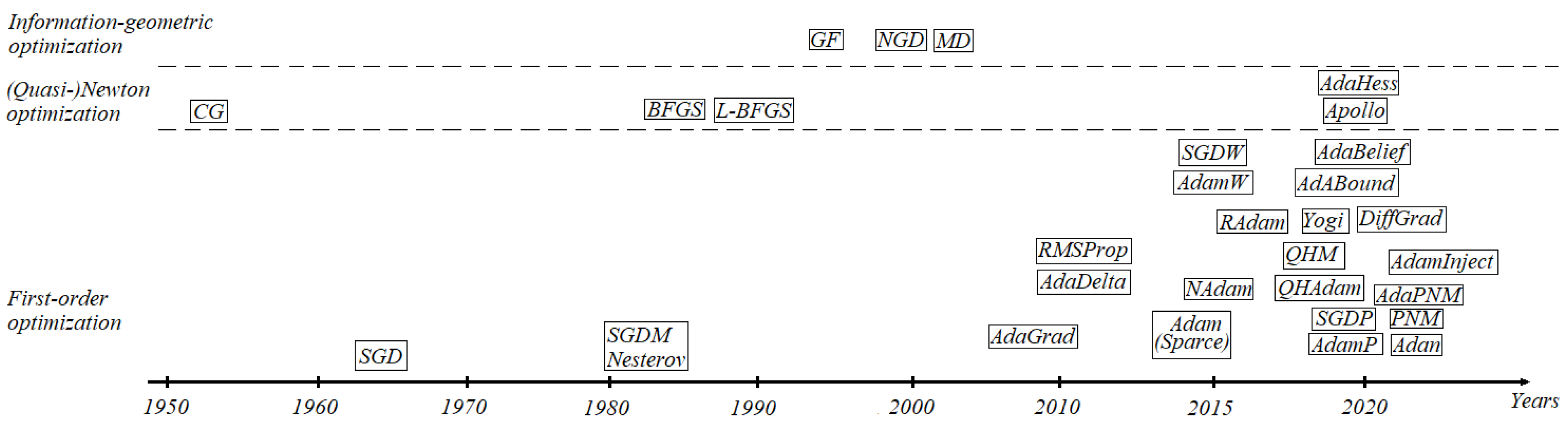
Table 1.
Summary of review papers on optimization algorithms in the theory of neural networks.
| Reference | Summary of Work | Limitations |
|---|---|---|
| [21] | A survey demonstrating first-order optimization algorithms in convolutional neural networks. | This survey presents only gradient-based optimization algorithms. They are well known and do not give any novel ideas for neural networks of different architecture. |
| [25] | A study reviewing the Grasshopper optimization algorithm, which is used for various problems in machine learning, image processing, wireless networking, engineering design, and control systems. | Regardless of the good presentation of the local, evolutionary, and swarm optimization algorithms, the author does not present global optimizers, which can improve the work of gradient-free neural networks, or other models in machine learning. |
| [26] | A survey studying various models, datasets, and gradient-based optimization techniques in deep meta-learning. | There are only stochastic gradient and adaptive moment estimation approaches, customized under conditions of meta-learning systems. |
| [27] | This survey describes the information-geometric optimization approach from probabilistic and geometrical points of view. There are new type manifolds with described Riemannian metrics and connections. | This review does not give exact application domains and lacks the mirror descent, which is a duality of the natural gradient descent. |
| [23] | This survey describes fractional optimization. There are are implied mathematical formulations of fractional error backpropagation. | This review mentions only Riemann–Liouville, Caputo, and Grunwald–Letnikov derivatives. |
| [28] | This review studies fractional, gradient-free, and information-geometric optimization algorithms. The author shows new types of manifolds with implied Riemannian metrics and connections. | Such a review does not mention other types of fractional derivatives. It considers only particle swarm optimization algorithms from gradient-free approaches and briefly describes the natural gradient descent with Fisher matrix approximation. |
Table 2.
List of conjugate gradient update parameters.
| CG Update Parameter | Authors | Year |
|---|---|---|
| Hestenes and Stiefel [83] | 1952 | |
| Fletcher and Reeves [84] | 1964 | |
| Daniel [85] | 1967 | |
| Polak and Ribière [86] and Polyak [87] | 1969 | |
| Fletcher [88], CD stands for “Conjugate Descent” | 1987 | |
| Liu and Storey [89] | 1991 | |
| Dai and Yuan [90] | 1999 | |
| Hager and Zhang [91] | 2005 |
Table 3.
List of Fisher information matrices for different probability distributions.
| Probability Density Function | Fisher Information Matrix | Probability Distribution |
|---|---|---|
| Gauss [115] | ||
| Multinomial [116] | ||
| Dirichlet [113,117] | ||
| for | Generalized Dirichlet [113] | |
| and | -zero matrix |
Table 4.
Potential function with corresponding Bregman divergences.
| Potential Function | Bregman Divergence | Algorithm |
|---|---|---|
| Gradient Descent | ||
| Exponentiated Gradient Descent |
Table 5.
Applications of optimization algorithm, divided into four types.
| Type of Optimization Algorithm | Optimizer | Application | Advantages | Disadvantages |
|---|---|---|---|---|
| SGD-type | SGD | PINN [136], SNN [137], CVNN [138], AE [139] | These optimizers are fast and can easily be customized. They still meet in many modern neural networks. The convergence rate is from to | These optimizers cannot reach the global minimum of the loss function. As the consequence, the training accuracy is decreasing. The majority do not have regret bound estimation. |
| AdaGrad | CNN [140] | |||
| AdaDelta | CNN [141], RNN [141], SNN [142] | |||
| RMSProp | CNN [143], RNN [144], SNN [145] | |||
| SGDW | CNN [37] | |||
| SGDP | CNN [38] | |||
| QHM | CNN [39] | |||
| NAG | CNN [146], RNN [147] | |||
| Adam-type | Adam | CNN [148], RNN [149], SNN [150], PINN [151], GNN [152] CVNN [153] | ADue to exponential moving averages and their modification, the optimization process is more accurate and rapid. The convergence rate can be improved from to . The number of parame ters is extended, which makes the optimization more controllable. | AOnly DiffGrad, Yogi, AdaBelief, AdaBound, and AdamInject can reach the global minimum of the loss function. They are appropriate for CNN and RNN. |
| AdamW | CNN [44] | |||
| AdamP | CNN [46] | |||
| QHAdam | CNN [49] | |||
| Nadam | CNN [51] | |||
| Radam | CNN [52] | |||
| DiffGrad | CNN [154], RNN [60], GNN [155] | |||
| Yogi | CNN [156], RNN [157] | |||
| AdaBelief | CNN [158], RNN [158], GNN [159] | |||
| AdaBound | CNN [160], RNN [161] | |||
| AdamInject | CNN [69] | |||
| PNM-type | PNM | CNN [73] | These optimizers are improved by positive–negative moment estimations, which help to reach the global extreme. | They are appropriate only for CNN. |
| AdaPNM | CNN [73] | |||
| Adan | CNN [74] | |||
| Newton | Newton approach | CNN [162] | These optimizers can reach the global minimum using less iterations. They can be extended on non-Euclidean domains. | They are appropriate only for
deep CNN, GNN, and PINN. The optimization process is too long. |
| CG | CNN [163], GNN [164] | |||
| Quasi-Newton | (L-)BFGS | PINN [165] | These optimzers are faster than Newton approaches. Their main ability is to achieve the global minimum in a short time. | These algorithms are not fast as first-order approaches. They are not useful for deep CNN. Only Apollo has a regret bound. |
| SR1 | CNN [166] | |||
| Apollo | CNN [97] | |||
| AdaHessian | CNN [98] | |||
| Information geometry | NGD | CNN [167], RNN [114], GNN [168], PINN [169], QNN [169] | These optimizers are novel and can be useful in neural networks of any type. The set of hyperparameters is controllable and wider than that in first-order approaches. | The mathematical model of these optimization methods is too complex for customization. Not many probability distributions and potential functions have been investigated for NGD and MD, respectively. |
| MD | CNN, RNN [170] |
Table 6.
Types of gradient-free optimization algorithm.
| Type of Optimization Algorithm | Optimizer |
|---|---|
| Local optimization | Hill Climbing [174], |
| Stochastic Hill Climbing [175], | |
| Simulated Annealing [176], | |
| Downhill Simplex Optimization [177] | |
| Global optimization | Random Search [178], |
| Grid Search [179], | |
| Random Restart Hill Climbing [180], | |
| Random Annealing [181], | |
| Pattern Search [182], | |
| Powell’s Method [183] | |
| Population-based optimization | Parallel Tempering [184], |
| Particle Swarm Optimization [185], | |
| Spiral Optimization [186], | |
| Evolution Strategy [187] | |
| Sequential model-based optimization | Bayesian Optimization [188], |
| Lipschitz Optimization [189], | |
| Tree of Parzen Estimators [190] |
Table 7.
Types of fractional derivatives on finite interval for gradient descent.
| Type of Fractional Derivatives | Formulas |
|---|---|
| Riemann–Liouville | , |
| , | |
| where | |
| Liouville–Sonine–Caputo | , |
| , | |
| where and | |
| Tarasov | , |
| , | |
| where and , | |
| Hadamard | , |
| , | |
| where , and | |
| Marchaud | , |
| , | |
| where | |
| Liouville–Weyl | , |
| , | |
| where and | |
| Sabzikar–Meerschaert–Chen | , |
| , | |
| where and | |
| Katugampola | , |
| , | |
| where and |
Disclaimer/Publisher’s Note: The statements, opinions and data contained in all publications are solely those of the individual author(s) and contributor(s) and not of MDPI and/or the editor(s). MDPI and/or the editor(s) disclaim responsibility for any injury to people or property resulting from any ideas, methods, instructions or products referred to in the content. |
© 2023 by the authors. Licensee MDPI, Basel, Switzerland. This article is an open access article distributed under the terms and conditions of the Creative Commons Attribution (CC BY) license (https://creativecommons.org/licenses/by/4.0/).
Share and Cite
MDPI and ACS Style
Abdulkadirov, R.; Lyakhov, P.; Nagornov, N. Survey of Optimization Algorithms in Modern Neural Networks. Mathematics 2023, 11, 2466. https://0-doi-org.brum.beds.ac.uk/10.3390/math11112466
AMA Style
Abdulkadirov R, Lyakhov P, Nagornov N. Survey of Optimization Algorithms in Modern Neural Networks. Mathematics. 2023; 11(11):2466. https://0-doi-org.brum.beds.ac.uk/10.3390/math11112466
Chicago/Turabian StyleAbdulkadirov, Ruslan, Pavel Lyakhov, and Nikolay Nagornov. 2023. "Survey of Optimization Algorithms in Modern Neural Networks" Mathematics 11, no. 11: 2466. https://0-doi-org.brum.beds.ac.uk/10.3390/math11112466
Note that from the first issue of 2016, this journal uses article numbers instead of page numbers. See further details here.