Matrix Factorization Techniques in Machine Learning, Signal Processing, and Statistics

Abstract

Compressed sensing is an alternative to Shannon/Nyquist sampling for acquiring sparse or compressible signals. Sparse coding represents a signal as a sparse linear combination of atoms, which are elementary signals derived from a predefined dictionary. Compressed sensing, sparse approximation, and dictionary learning are topics similar to sparse coding. Matrix completion is the process of recovering a data matrix from a subset of its entries, and it extends the principles of compressed sensing and sparse approximation. The nonnegative matrix factorization is a low-rank matrix factorization technique for nonnegative data. All of these low-rank matrix factorization techniques are unsupervised learning techniques, and can be used for data analysis tasks, such as dimension reduction, feature extraction, blind source separation, data compression, and knowledge discovery. In this paper, we survey a few emerging matrix factorization techniques that are receiving wide attention in machine learning, signal processing, and statistics. The treated topics are compressed sensing, dictionary learning, sparse representation, matrix completion and matrix recovery, nonnegative matrix factorization, the Nyström method, and CUR matrix decomposition in the machine learning framework. Some related topics, such as matrix factorization using metaheuristics or neurodynamics, are also introduced. A few topics are suggested for future investigation in this article.

1. Introduction

Matrix factorization is widely used for inferring the structure in multivariate data. Given a noisy measurement of the product of two matrices, the matrix factorization problem aims to estimate the original matrices. It represents an observed data matrix $\mathbf{Y}\in {\mathbb{R}}^{m\times n}$ as

$$\mathbf{Y}={\mathbf{L}}^T\mathbf{F}+\mathbf{E},$$

(1)

where $\mathbf{L}\in {\mathbb{R}}^{k\times m}$, $\mathbf{F}\in {\mathbb{R}}^{k\times n}$, and the residual matrix is denoted as $\mathbf{E}\in {\mathbb{R}}^{m\times n}$, which is usually assumed to have normally distributed entries. For factor analysis, $\mathbf{L}$ is referred to as the loadings, and $\mathbf{F}$ is referred to as the factors.

Matrix factorization is a bilinear inverse problem in individual matrices. Model (1) has many applications. For the matrix completion problem, the estimations of $\mathbf{L}$ and $\mathbf{F}$ from partially observed $\mathbf{Y}$ provide a natural and simple way to estimate the missing entries; this is a typical scenario in matrix completion tasks. Another wide range of applications involve inferring and summarizing the structures in multivariate data in $\mathbf{Y}$, where each row of $\mathbf{Y}$ is approximated by a linear combination of the rows of $\mathbf{F}$, which are referred to as factors, corresponding to factor analysis, the principal component analysis (PCA), or dictionary learning.

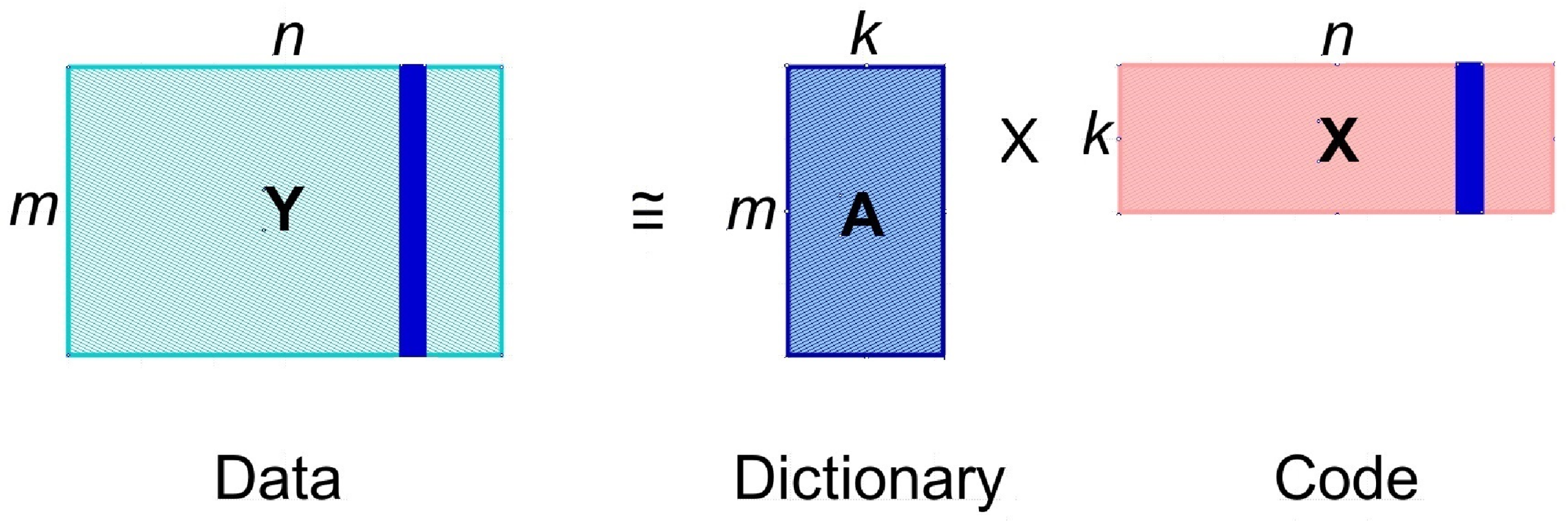
The dictionary $\mathbf{A}$, corresponding to ${\mathbf{L}}^T$ in (1), is subject to some constraints. A prominent example is PCA [1], where $\mathbf{A}$ has orthogonal columns, representing the subspace where the signal in the given class is contained. Another example is sparse coding, where $\mathbf{A}$ typically consists of normalized columns that form an overcomplete basis of the signal space, and the signal $\mathbf{x}\in {\mathbb{R}}^k$, corresponding to $\mathbf{F}$ degenerating into a column vector (i.e., $n=1$), is assumed to be sparse. Matrix factorization is more commonly, represented by

$$\mathbf{Y}=\mathbf{A}\mathbf{X}+\mathbf{E},$$

(2)

where $\mathbf{Y}\in {\mathbb{R}}^{m\times n}$ is the data matrix, $\mathbf{A}\in {\mathbb{R}}^{m\times k}$ is the dictionary matrix, and $\mathbf{X}\in {\mathbb{R}}^{k\times n}$ is the code matrix. Each column of $\mathbf{Y}$ is approximated by a linear combination of the columns of $\mathbf{A}$, where the coefficients are given by the corresponding column of matrix $\mathbf{X}$. This is illustrated in Figure 1.

Matrix factorization provides a low-rank approximation of a matrix. It arises in many machine learning and signal processing applications [2], such as singular value decomposition (SVD), factor analysis, PCA, blind source separation, independent component analysis (ICA), blind matrix calibration, dictionary learning, low-rank matrix completion, nonnegative matrix factorization (NMF), C-means clustering [3], unsupervised representation learning, and so on. A penalty or prior distribution is usually used to achieve sparse representations (e.g., sparse factor analysis and sparse PCA). As a related concept, matrix decomposition aims to recover, from a matrix, a low-rank matrix and a sparse matrix. These techniques fall under the category of unsupervised learning in the machine learning framework [4].

Representation learning is a concept behind many machine learning applications, including the deep learning framework. In the context of representation learning, dictionary learning is sometimes referred to as sparse coding. Sparse coding has been proposed as a theory for modeling the visual cortex and as an unsupervised algorithm for learning representations. These methods are widely used for feature extraction and knowledge discovery. Low-rank matrix approximation is a ubiquitous problem in data processing.

Compressed sensing is a powerful framework used for acquiring sparse signals. Learning a sparsifying dictionary or transforming from compressive measurements [5,6] requires fewer equations to determine the unknowns, compared to matrix factorization. Dictionary learning aims to find a good sparse representation for a dataset. It is a matrix factorization problem with a sparsity constraint. Compressive blind source separation [7] is another matrix factorization problem with a sparsity constraint. These problems can be solved by recovering a sparse and low-rank matrix from its linear measurements. NMF can be made equivalent to some clustering problems by reframing them slightly [8]. NMF and spectral clustering are two popular clustering techniques. However, NMF cannot deal with nonlinear data, and spectral clustering relies on post-processing.

Crowdsourcing is a scalable approach to collecting data from humans. Through crowdsourcing platforms such as Amazon Mechanical Turk, a large number of data tasks are assigned to workers for binary or multiclass labeling. The goal is to estimate the unknown ground truth from the input of the various workers. The unknown labels can be estimated through aggregation, such as majority voting or weighted majority voting.

Sparsity is a natural property that consists of many real signals. In the human brain, very few neurons (1–4%) are active at any time [9]. Many observed response properties in the primary visual cortex (V1), such as the classical receptive field structure [10] and nonclassical response modulations [11], are accounted for by using the sparse coding model of the primary visual cortex. In the sparse coding model, most natural images are encoded by very few learned dictionary elements, and high-dimensional visual inputs can be represented by a small number of active cortical neurons [10].

Sparse coding involves learning an overcomplete set of basis vectors, where each data point is represented as a sparse combination of the basis vectors. On the contrary, sparse recovery aims to reconstruct sparse signals from an underdetermined set of compressed linear measurements.

The recovery of sparse signals corrupted by additive noise covers a wide range of applications, such as image inpainting, super-resolution, signal separation, and recovery of signals that are impaired by clipping, impulse noise, or narrowband interference.

For linear inverse or compressed sensing problems, a series of representer theorems give the generic form of the solution, which depends on whether $L_1$- or $L_2$-norm regularization is under consideration [12]. $L_1$-norm solutions are proven to be intrinsically sparse, and the use of the $L_1$-norm regularization is much more favorable for incorporating prior knowledge compared to the $L_2$-norm scenario. $L_1$-norm has long been used for pruning neural network architecture [13].

Compressed sensing, also known as compressive sampling, is a recent sampling method [14,15]. If a signal is sufficiently sparse, it can be exactly reconstructed from very few random measurements. Compressed sensing serves as an alternative to classical Shannon/Nyquist sampling for sparse or compressible signals, allowing for the perfect recovery of sparse signals using only a small number of random measurements. Compressible signals can be well approximated by sparse signals. A non-sparse signal can be compressed by using compressive covariance sensing [16], and its second-order statistics can be recovered from the compressed signal without sparsity constraint.

Low-rank representation is usually used to recover data from corruption or outliers. PCA is the best low-rank representation in terms of $L_2$ errors. By minimizing the $L_2$-norm error, data are projected onto the fixed-rank low-dimensional space. Robust PCA [17] and GoDec [18,19] decompose data into low-rank components and sparse components that capture corruptions.

Matrix completion [20] recovers a matrix from a subset of its entries. It had been prevalent in computer vision, statistics, collaborative filtering, and manifold learning in the last decade. It is an ill-posed problem. A common constraint is applied to the underlying matrix. The task is formulated as a low-rank matrix approximation problem. The method is related to compressed sensing. The values of matrix entries may be discrete or quantized, such as in the Netflix problem and recommender systems.

Many real-life data or physical signals are represented by nonnegative numbers. When analyzing mixtures of such data, nonnegativity constraints on the individual components are applied. Nonnegative PCA, nonnegative ICA, and NMF [21] are techniques used for the analysis of such data, where nonnegative data are represented as nonnegative linear combinations of nonnegative bases. Nonnegativity is inspired by neuronal properties, such as the firing rate representation and signed synaptic weight [21].

The inferior temporal cortex is a critical region in the primate visual cortex for object recognition. Object representation in this region has two prominent features. An object is represented by a combination of the activities of columnar clusters of neurons, where each cluster represents component features or parts of objects [22].

NMF [21,23] factorizes a matrix as a product of two matrices, whose elements are all nonnegative. Nonnegativity prevents mutual cancellation between basis functions and, thus, generates a parts-based representation, in agreement with human thinking. NMF can be used for tasks such as blind source separation (BSS) of images and nonnegative signals [24], spectra recovery [25], feature extraction, and clustering [26].

Canonical correlation analysis, SVD, PCA, and ICA are classical matrix factorization methods, derived by the low-rank approximation to a matrix by minimizing the squared error. Latent semantic indexing [27] is an application that uses SVD for automatic indexing and retrieval. We do not describe them here. In this paper, we provide a survey on the recent matrix factorization techniques that are prevalent in machine learning and signal processing. In Section 2, we describe compressed sensing. Section 3 introduces sparse coding and dictionary learning. Section 4 extends sparse coding to matrix completion. In Section 5, low-rank representation is reviewed. In Section 6, NMF is introduced. Section 7 introduces techniques for symmetric positive semidefinite matrix approximation, including the Nyström method. Section 8 describes the CX Decomposition and CUR decomposition. Finally, a summary is given in Section 9.

2. Compressed Sensing

Compressed sensing seeks to recover sparse or compressible signals from undersampled linear measurements [15,28]. A sparse or compressible high-dimensional signal can be projected onto a low-dimensional space when applying a random observation matrix. Compressibility of data and acquisition of incoherent measurements are the two fundamental properties underlying compressed sensing.

Given a signal $\overrightarrow{x}$, if $\overrightarrow{\alpha }={\mathsf{\Phi }}^T\overrightarrow{x}$ is sparsely distributed for any dictionary $\mathsf{\Phi }$, $\overrightarrow{x}$ is said to be compressible.

2.1. Signal Model

In compressed sensing, a signal with N samples, $\overrightarrow{x}\in {\mathbb{R}}^N$, is derived from a set of linear measurements

$$\overrightarrow{y}=\mathbf{A}\overrightarrow{x}+\overrightarrow{n},$$

(3)

where $\mathbf{A}\in {\mathbb{R}}^{M\times N}$ denotes a random sampling, sensing, or measurement matrix, $\overrightarrow{y}\in {\mathbb{R}}^M$ is a measurement vector with M measurements, $M<N$, and $\overrightarrow{n}\in {\mathbb{R}}^M$ is noise.

The problem (3) is underdetermined. When the norm of each column of $\mathbf{A}$ is unity, all of the columns form an incomplete basis with $M\ll N$.

In order to preserve the information in sparse or compressible signals $\overrightarrow{x}$, and to ensure the stable recovery of such signals, $\mathbf{A}$ has to satisfy the so-called restricted isometry property (RIP) [14].

$\mathbf{A}$ should also satisfy the incoherence property. $M=O(klnN)$ measurements are sufficient for perfectly reconstructing a k-sparse vector $\overrightarrow{x}$, if $\mathbf{A}$ is perfectly incoherent (e.g., uniformly random Gaussian measurements).

Compressed sensing achieves the stable recovery of compressible, noisy signals by solving the $L_0$-norm regularized inverse problem, or the corresponding computationally tractable $L_1$-norm problem

$$\underset{\overrightarrow{x}}{min}\parallel \overrightarrow{x}{\parallel }_1\mathrm{or}\parallel \overrightarrow{x}{\parallel }_0\mathrm{subject} \mathrm{to}{\parallel \mathbf{A}\overrightarrow{x}-\overrightarrow{y}\parallel }_2^2\le {\epsilon }^2,$$

(4)

where $L_0$-norm $\parallel \overrightarrow{x}{\parallel }_0$ counts the nonzero entries in $\overrightarrow{x}$, $L_1$-norm is the convex envelope of $L_0$-norm, $\parallel \overrightarrow{x}{\parallel }_1={\sum }_{i=1}^N\left|x_i\right|$, and $\epsilon$ is a tolerance.

The $L_0/L_1$-regularized least squares (LS) approach is used to deal with linear inverse problems under sparsity constraints. Linear programming (LP) has the best sparsity–undersampling trade-off, at a cost of high computation complexity. The approximate message-passing algorithm [29] is an iterative thresholding algorithm corresponding to the LP procedure, but is dramatically faster.

The east absolute selection and shrinkage operator (LASSO) [30] and approximate message passing [29] are low-complexity reconstruction procedures. By minimizing a weighted sum of the residual norm and a regularization term $\parallel \overrightarrow{x}{\parallel }_1$, LASSO can reconstruct sparse solutions and recover the sparsity pattern exactly as the number of observations increases, asymptotically with probability one.

Standard compressed sensing guarantees robust signal recovery from $O(klog\frac{N}{k})$ measurements with provable performance guarantees [31]. Based on a model-based compressed sensing theory, two recovery algorithms incorporating wavelet trees and block sparsity are proven to offer robust recovery from $O\left(k\right)$ measurements [31].

In [32], sensing vectors are selected independently at random from a probability distribution $\mathcal{F}$. If $\mathcal{F}$ obeys an incoherence property and an isotropy property, approximately sparse signals can be faithfully recovered from a minimum number of noisy measurements. The recovery does not require the RIP to hold near the sparsity level, and it also does not need a random model for the signal. A k-sparse signal can be faithfully recovered from about $klogN$ noisy Fourier coefficients.

When the measurements are obtained using a matrix with i.i.d. Gaussian entries, the weighted $L_1$-norm minimization recovers the sparse signal with overwhelmingly high probability [33]. For any stationary process satisfying certain mixing conditions, if the sampling rate is greater than the information dimension of the source process, the minimum entropy pursuit (MEP) optimization approach for universal compressed sensing can reliably recover the source vector almost losslessly, without any prior information about its distribution [34].

2.2. RIP, ERC, and MIP

Conditions used in the compressed sensing literature include the RIP [28], exact recovery condition (ERC) [35], and mutual inheritance property (MIP).

2.2.1. RIP

The RIP of sampling matrices is a sufficient condition for the reliable reconstruction of sparse signals [15]. RIP matrices can be constructed from binary vectors [36]. Both the algorithmic and constructive aspects were pursued to connect to error correction codes [37,38].

A k-sparse vector $\overrightarrow{x}$ has, at most, k nonzero entries, $\parallel \overrightarrow{x}{\parallel }_0\le k$. For any k-sparse vector $\overrightarrow{x}\in {\mathbb{R}}^N$, if there exists a constant $\delta \in (0,1)$, such that [14,39]

$$(1-\delta )\parallel \overrightarrow{x}{\parallel }_2^2\le \parallel \mathbf{A}\overrightarrow{x}{\parallel }_2^2\le (1+\delta ){\parallel \overrightarrow{x}\parallel }_2^2,$$

(5)

a sensing matrix $\mathbf{A}\in {\mathbb{R}}^{M\times N}$ is said to satisfy the k-restricted isometry property (k-RIP).

The minimum of all $\delta \in (0,1)$, denoted as ${\delta }_k$, is referred to as the kth-order restricted isometry constant (RIC), or simply RIC, of $\mathbf{A}$. A smaller RIC corresponds to a transformation closer to an isometry. The RIC has monotonicity properties, ${\delta }_k\le {\delta }_{2k}$. Via a RIP analysis, one can find the maximum sparsity order k that guarantees the recovery of all sparse vectors.

k-RIP ensures that all $M\times k$ submatrices of $\mathbf{A}$ approximately satisfy the isometry property and, hence, distance preserving. When M is close to k, maximal signal compression is achieved. RIP can be used to measure the orthogonality of column vectors of a dictionary. The problem of determining whether $\mathbf{A}$ has RIP for any accuracy is proven to be NP-hard [40]. Constructing RIP matrices deterministically is a hard problem [41], but RIP matrices can be generated with high probability by simple random methods [42,43].

The RIP analysis shows that Gaussian measurement matrices are information-theoretically optimal since the required number of measurements for sparse recovery is minimal [28,44]. A k-RIP matrix must have at least $M=\mathsf{\Omega }(klog\frac{N}{k})$ rows. That is, $M=\mathsf{\Omega }(klog\frac{N}{k})$ samples are required for any recovery algorithm to approximate the signal $\overrightarrow{x}$ with an accuracy expressed by the $L_1$- or $L_2$-norm [45,46]. This bound is applicable to non-k-sparse signals. Random Gaussian or Bernoulli matrices provide, with high probability, the best-known accuracy for recovery that matches this lower bound [28,47,48].

When most $M\times k$ submatrices define a near-isometric map of ${\mathbb{R}}^k$ into ${\mathbb{R}}^M$, a matrix has a statistical RIP of order k [49]. Statistical RIP is particularly useful for the sparse signal recovery of deterministic sensing matrices. For many existing deterministic sampling matrices, $M=O\left(k\right)$ rows guarantee k-statistical RIP [49]. With the conditions of statistical RIP and statistical incoherence, stable sparse recovery by a basis pursuit can be proved [49].

The k-RIP concept is extended to the case of the $L_p$-norm [50]. For every $1\le p<\infty$, almost tight bounds on the minimum number of rows, M, which are necessary for the RIP to hold, as well as almost tight bounds for the column sparsity of RIP matrices, are obtained [50].

2.2.2. ERC

The ERC is a necessary and sufficient condition for exact support recovery in a worst-case analysis [35]. If a subset of atoms satisfies the ERC, then it can be recovered from any linear combination of the atoms in, at most, k steps. The ERC necessarily holds when the latter conditions are fulfilled since the ERC is a worst-case necessary condition for exact recovery.

When the ERC is met, the orthogonal least squares (OLS) algorithm is guaranteed to exactly recover unknown support in, at most, k iterations, where k denotes the support cardinality [51]. The authors of [51] provide a closer look at the analysis of both orthogonal matching pursuit (OMP) and OLS when the ERC is not fulfilled. The existence of dictionaries for which some subsets are never recovered by OMP is proved. This phenomenon also appears with basis pursuit, where support recovery depends on the sign patterns, but it does not occur for OLS. None of the OMP, OLS, and basis pursuit algorithms is uniformly better than the others, but for correlated dictionaries, OLS may achieve guaranteed exact recovery in fewer iterations compared to OMP.

2.2.3. MIP

The conditioning of the dictionary characterizes how different its atoms are [52]. The performance of a sparse recovery algorithm is affected by the conditioning. The conditioning of a matrix is commonly measured by its condition number, which characterizes the sensitivity of the solution of a system of linear equations to noise.

Mutual coherence and the RIP constant can be seen as two measures of the conditioning of the dictionary. A large mutual coherence corresponds to two similar atoms, implying a bad conditioning in the dictionary and, hence, difficulties in finding the sparse solution.

One common assumption in studying the statistical performance of the estimators is the MIP that requires the mutual incoherence $\mu \left(\mathbf{A}\right)$ to be small [53,54,55]. Mutual coherence [55,56] is defined as the maximum value among all the correlation coefficients of normalized columns of a dictionary $\mathbf{A}$,

$$\mu \left(\mathbf{A}\right)=\underset{i\ne j}{max}|<{\overrightarrow{a}}_i,{\overrightarrow{a}}_j>|,$$

(6)

where ${\overrightarrow{a}}_i$ and ${\overrightarrow{a}}_j$ are two columns of $\mathbf{A}$.

If the $L_0$-norm problem has a k-sparse solution ${\overrightarrow{x}}_0$, for which $k<\frac{1}{2}(1+\mu {\left(\mathbf{A}\right)}^{-1})$, then it is the unique solution for both the $L_1$-norm and $L_0$-norm minimization problems [55,56]. This condition can be replaced by ERC, but ERC is not easy to check because it depends on unknown support. The condition $k<\frac{1}{2}(1+{\mu }^{-1})$ is a sufficient condition for ERC [35] to hold, and is easy to check.

The MIP implies RIP and ERC but the converse is not true. For OMP, support recovery was considered in the noiseless case [35], where the MIP condition $\mu <\frac{1}{2k-1}$ is a sufficient condition for exactly recovering a k-sparse signal $\overrightarrow{x}$ in the noiseless case. This condition is, in fact, sharp [57]. Under the MIP condition $\mu <\frac{1}{2k-1}$ and a condition on the minimum magnitude of the nonzero coordinates of $\overrightarrow{x}$, the support of $\overrightarrow{x}$ can be recovered exactly by the OMP algorithm in the bounded noise cases and with high probability in the Gaussian case [58].

2.3. Sparse Recovery

A high-dimensional k-sparse signal $\overrightarrow{x}\in {\mathbb{R}}^N$ can be expressed as a linear combination of M atoms ($2k\le M\le N$), defined by the sensing matrix $\mathbf{A}={\left[{\overrightarrow{a}}_1,{\overrightarrow{a}}_2,\dots ,{\overrightarrow{a}}_M\right]}^T\in {\mathbb{R}}^{M\times N}$, as given by (3).

Nonlinear reconstruction algorithms are derived from the $L_0$-norm regularized problem,

$$\underset{\overrightarrow{x}\in {\mathbb{R}}^N}{min}\mathsf{\Psi }\left(\overrightarrow{x}\right)=\frac{1}{2}\parallel \mathbf{A}\overrightarrow{x}-\overrightarrow{y}{\parallel }^2\mathrm{subject} \mathrm{to}{\parallel \overrightarrow{x}\parallel }_0\le k.$$

(7)

When $\overrightarrow{y}$ is a k-sparse signal, the problem is known as the k-exact-sparse problem.

The $L_0$-norm regularized problem (4) is non-convex and NP-hard. It has many local minima; when there is zero noise, a unique global minimum is the k-sparse vector ${\overrightarrow{x}}^{*}$ [59]. Many suboptimal algorithms approximate its solution. They recover the true value of ${\overrightarrow{x}}^{*}$ when $\overrightarrow{x}$ is sufficiently sparse and the columns of $\mathbf{A}$ are incoherent.

The $L_0$-norm problem (7) is usually formulated as

$$\underset{\overrightarrow{x}\in {\mathbb{R}}^N}{min}{\parallel \overrightarrow{x}\parallel }_0\mathrm{subject} \mathrm{to}\mathbf{A}\overrightarrow{x}=\overrightarrow{y}.$$

(8)

The $L_0$-norm problem (8) is NP-hard [60]. It is usually relaxed, and is reconstructed via the $L_1$-norm minimization problem [15,61]:

$$\underset{\overrightarrow{x}\in {\mathbb{R}}^N}{min}{\parallel \overrightarrow{x}\parallel }_1\mathrm{subject} \mathrm{to}\mathbf{A}\overrightarrow{x}=\overrightarrow{y}.$$

(9)

This is the basis pursuit method [62]. By imposing appropriate constraints on $\mathbf{A}$, the basis pursuit generates the exact recovery of $\overrightarrow{x}$.

Sparsity is a basic type of regularization. Sparse approximation finds a k-sparse signal ${\overrightarrow{x}}^{*}$ to approximate $\overrightarrow{y}=\mathbf{A}\overrightarrow{x}$ while $k\ll N$. Compressed sensing is a type of sparse approximation problem.

Compared with $L_1$-norm regularization, sparsity is better achieved with $L_0$-norm penalties based on experiments [63]. Under the RIP condition, the solutions by $L_1$-norm and $L_0$-norm regularization are equal [44]. However, $L_1$-norm regularization over-penalizes large coefficients, yielding biased estimation [64,65].

$L_p$-norm ($0<p<1$) is non-convex. Alternatively, $L_p$-norm ($0<p<1$) is an approximation to the $L_0$-norm,

$$\underset{\overrightarrow{x}\in R^N}{min}{\parallel \overrightarrow{x}\parallel }_p^p\mathrm{subject} \mathrm{to}\mathbf{A}\overrightarrow{x}=\overrightarrow{y}.$$

(10)

Regarding the random Gaussian matrix $\mathbf{A}$, the recovering ability of the $L_p$-norm minimization ($p\in [0,1)$) was investigated in [66]. When $\alpha =\frac{M}{N}\to 1$, the sharp threshold of the sparsity ratio differentiates the success and failure via $L_p$-norm minimization. $L_p$-norm minimization succeeds below the threshold. For strong recovery, the threshold decreases strictly from $0.5$ to $0.239$ as p rises from 0 to 1, whereas for weak recovery, the threshold is $2/3$ for $p\in [0,1)$. The threshold is 1 for $L_1$-norm minimization. $L_p$-norm minimization can return a denser solution compared to $L_1$-norm minimization. For any $\alpha \in (0,1)$, thresholds of the sparsity ratio for strong recovery and weak recovery are, respectively, provided in [66]. For strong recovery, $L_p$-norm minimization has a higher threshold with smaller p; for sectional recovery, the threshold is the same for all p; for weak recovery, $L_1$-norm minimization can outperform $L_p$-norm minimization. $L_1$-norm minimization generally outperforms $L_p$-norm minimization for sparse recovery.

Suboptimal signal recovery methods are categorized into greedy pursuit, thresholding, and convex relaxation methods. Greedy pursuit methods, such as matching pursuit [67], OMP [68], OLS [69], subspace pursuit [70], and compressive sampling matching pursuit (CoSaMP) [71], tackle the $L_0$-norm problem directly. Iterative hard thresholding (IHT) is a thresholding method for the $L_0$-norm problem [72]. Convex relaxation methods, such as gradient projection [73,74], accelerated proximal gradient [75], iterative reweighted method [76], homotopy method [77], and least angle regression [78], solve the $L_1$-norm problem, and there are also relaxation methods for the $L_p$-norm problem [79].

Basis pursuit [62] is a greedy sparse approximation technique used for solving the $L_1$-norm problem. For a given set of basis vectors, the method solves the optimization problem by greedily searching for vectors to add or remove. OMP [68], also known as the fully corrective forward greedy selection or simply the forward selection [60], is a simple and effective greedy algorithm for sparse recovery/approximation. The atom selection steps in matching pursuit and the Frank–Wolfe algorithm are very similar [80]. If k is small enough, then at each iteration, both matching pursuit and OMP select an atom indexed by the support, thus ensuring recovery properties [35,81]. Under the condition $k<\frac{1}{2}(1+{\mu }^{-1})$, it has been proven that matching pursuit shows an exponential rate of convergence, and that OMP reaches convergence after exactly k iterations [35]. Under this same condition, it was proved that the Frank–Wolfe algorithm converges exponentially beyond a certain iteration, even though the function is not strongly convex [80].

CoSaMP and subspace pursuit improve upon OMP by selecting multiple coordinates and incorporating a pruning step at each iteration, and sparse signal recovery was based on RIP [28]. This selection strategy results in an optimal sample complexity. At each iteration, CoSaMP first prunes the gradient, then solves an LS program restricted on a small support set; finally, hard thresholding is implemented to form a k-sparse iterate for future updates. As a greedy method, the hard thresholding pursuit adds and prunes indices on a list [82].

Compared to batch solvers, $L_1$-norm-based stochastic algorithms struggle to preserve the sparse structure of the solution [83].

If the optimal solution is sufficiently sparse, the problems (9) and (8) have approximately the same solution [44,48,62,68]. The problem (9) can be effectively solved by LP methods.

For the $L_p$-norm problem, projected gradient [84], iterative reweighted method [85], and approximate operator [86,87] can be used. These methods converge to a global minimum for proper initial points, which is easier to choose for larger p [84].

For compressed sensing, a sparse signal is represented in a finite discrete dictionary. The true parameters, however, may be from a continuous dictionary. Thus, the loss of sparsity arises from spectral leakage along the Dirichlet kernel [88]. From a small random subset of its N time-domain samples, spectrally compressed sensing can recover a spectrally sparse signal. It is assumed that a signal can be represented as the sum of k complex multidimensional sinusoids.

Assuming that the signal frequencies are on a grid, it is guaranteed that the spectrally sparse signal can be faithfully recovered from $O(klogN)$ random time-domain samples by using compressed sensing algorithms derived from $L_1$-norm minimization [44,61], even in the presence of bounded noise [47] or sparse outliers [89]. Additionally, a total-variation norm minimization method can recover a sparse signal from low-frequency samples [90].

In [91], a greedy method for the sparse recovery of linear measurements corrupted by highly impulsive noise is designed to solve a minimum dispersion optimization problem by adopting the family of symmetric alpha-stable distributions.

Sparse recovery algorithms with invariance properties are less affected when the sensing matrix (i.e., the dictionary) is ill-conditioned [52]. There implicitly exists an equivalent well-conditioned problem. Some sparse recovery algorithms, such as smoothed $L_0$-norm [92], basis pursuit, FOCUSS [93], and hard thresholding algorithms, are invariant, while others, such as matching pursuit and the spectral projected gradient for $L_1$-norm minimization (SPGL1) [94], are not.

2.4. Iterative Hard Thresholding

A simple greedy technique known as IHT [72,95] can generate the steepest descent steps that are feasible for the $L_1$-norm problem (9). This is achieved by utilizing hard thresholding to project steps along the negative gradient direction of $\mathsf{\Psi }$ onto the $L_0$-norm constraint. In the hard thresholding method, all but the k largest magnitude elements of a vector are set to zero. IHT utilizes a proximal-point technique at each iteration, and it implements gradient projection with a constant step size. In normalized IHT [96], a self-adaptive step size is adopted to guarantee stability and performance.

In case the spectral norm of $\mathbf{A}$ is less than one, IHT converges to a fixed point of (9) [72]. IHT guarantees stable recovery, provided that $\mathbf{A}$ has RIP [95]. There are also other RIP-based recovery conditions for IHT [82] and normalized IHT [96]. The theory for compressed sensing assumes that samples are taken from linear measurements. Under similar conditions, IHT accurately recovers sparse or structured signals from a few nonlinear observations [97]. Global linear convergence for IHT is guaranteed from theory works based on matrix completion, which is based on standard properties of incoherence and uniform sampling.

For any $\mathbf{A}$, sufficient conditions for the convergence of IHT to a fixed point, as well as necessary conditions for the existence of fixed points, are given in [98]. Sparse signal recovery analysis can be performed using these conditions. The analysis has been extended to normalized IHT. A theoretical analysis of normalized IHT, when both $\mathbf{A}$ and $\overrightarrow{y}$ are quantized, is given in [99], and it is proved that a low-precision normalized IHT can provide recovery guarantees under mild conditions.

IHT [72] and iterative soft-thresholding [100] algorithms are for the $L_0$- and $L_1$-norm problems, respectively. Half thresholding [86] is given for $p=\frac{1}{2}$. These iterative thresholding algorithms are efficient for high-dimensional problems, and it is also relatively easy to specify the regularization parameter.

In the proximal gradient homotopy method, the solutions of the regularized problem are computed and traced along a continuous homotopy path, and the selection of a regularization parameter is not needed. IHT, when combined with the homotopy technique, avoids the requirement of choosing a regularization parameter [101].

The hard thresholding pursuit [82] is an iterative greedy selection procedure used for the sparse recovery of the $L_0$-norm problem. As a combination of CoSaMP and IHT, it outperforms both methods in terms of the RIP. The exact recovery of sparse signals is theoretically justified under conditions of restricted strong condition number bounding [102]. In [103], the hard thresholding pursuit is generalized to sparsity-constrained convex optimization. The algorithm includes iterations of a gradient descent step and a hard thresholding step.

Iterative thresholding algorithms have much lower computational complexity per iteration and lower storage requirements than interior point methods. The recursions are modifications of the gradient method used to solve a linear system but consist of a (hard or soft) shrinkage operator to promote the sparsity of the estimate at each iteration. Hard thresholding algorithms are always orders of magnitude faster than convex programs [104].

A theoretical analysis of hard thresholding algorithms is given in [105]. A tight bound used for characterizing hard thresholding algorithms is derived, and RIP and sparsity parameters are related. Parsimonious solutions are guaranteed by following a stochastic hard thresholding procedure. Global linear convergence is proved under certain mild assumptions [105].

IHT is a first-order greedy selection method that minimizes the primal formulation. The original non-convex problem can be equivalently or approximately solved in a concave dual formulation under certain conditions. The dual IHT algorithm [106] is a super-gradient ascent method used to solve the non-smooth dual problem. Dual IHT is superior to IHT in model estimation accuracy and computational efficiency.

The GradMP algorithm [107] generalizes the idea of CoSaMP [71]. Stochastic IHT and stochastic GradMP [108] are two stochastic variants of greedy algorithms. The expected linear convergence towards the solution within a specified tolerance is proven, providing methods that often outperform their deterministic counterparts. In stochastic GradMP [108], at each iteration, only the gradient of a function is evaluated, a subspace is searched based on the previous estimate, and then a new solution is obtained via solving a convex low-dimensional sub-optimization problem.

Sparse convex optimization solves the optimization of a convex function subject to a sparsity constraint $k\le k^{*}\gamma$, where $k^{*}$ is a target sparsity and $\gamma \ge 1$ is an approximation factor. The adaptively regularized hard thresholding (ARHT) algorithm [109] brings the bound down to $\gamma =O\left(\kappa \right)$, with $\kappa$ being the restricted condition number, which is tight for a general class of algorithms, including IHT, OMP, and LASSO. ARHT is comparable to the most efficient greedy algorithms in terms of runtime, as it requires a single function minimization per iteration. ARHT provides a strong trade-off between the RIP condition and the solution sparsity.

Newton step-based IHT and Newton step-based hard thresholding pursuit adopt the Newton-like search direction instead of the steepest descent direction [110]. Sufficient guarantees for these algorithms are established in terms of the RIP of a sensing matrix.

A class of distributed iterative thresholding algorithms for $L_0/L_1$-regularized LS optimization problems is presented in [111]. By introducing a suitably distributed and regularized LS functional, it has been demonstrated that the algorithms reach their minima based on the dynamical systems theory [111].

2.5. Orthogonal Matching Pursuit

OMP [68], also known as forward stepwise regression, is a fast greedy algorithm. At each iteration, the algorithm selects the column from matrix $\mathbf{A}$ that is maximally correlated with the current residual and adds it to the set of selected columns. That is, at each iteration, one new element of the dictionary is added and one orthogonal projection is made. The residuals are updated by projecting the observations $\overrightarrow{y}$ onto the linear subspace that is spanned by the columns already selected, and then the algorithm iterates. The stopping rule depends on the noise structure.

OMP can recover a k-sparse signal $\overrightarrow{x}\in {\mathbb{R}}^N$ from incomplete measurements $\overrightarrow{y}\in {\mathbb{R}}^M$ obeying (3), with $k\ll M\ll N$. OMP recovers the true signal with high probability for random matrices, including Gaussian, but it may fail for some deterministic sensing matrices [35,112].

OMP, such as OLS, constructs the dictionary in an incremental way. By adding one index to the list at a time, the support of the underlying sparse signal is identified, and the sparse coefficients over the enlarged support are estimated. In OLS, a candidate that leads to the most significant decrease in residual power is selected. In comparison, in OMP, a column that is the most strongly correlated to the residual is chosen. OLS outperforms OMP in terms of convergence, at a cost of higher computational complexity [51].

Some greedy methods, such as stagewise OMP [113], regularized OMP [114], and generalized OMP [115] (also referred to as the orthogonal super greedy algorithm [116]) add multiple indices per iteration. At each iteration, candidates are identified according to correlations between the residual vector and columns of $\mathbf{A}$. The multipath matching pursuit [117] extends OMP by recovering sparse signals with a tree-searching strategy. At each iteration, multiple candidate paths are traced and extended, and the candidate that minimizes the residual power is chosen. Multiple OLS [118] extends OLS by selecting multiple indices at each iteration, leading to convergence in fewer iterations. Stable sparse recovery can be guaranteed, provided that the signal-to-noise ratio (SNR) grows linearly with the sparsity level k of the input signals.

When MIP or SNR satisfies certain conditions, OLS and multiple OLS methods reliably recover k-sparse signals in, at most, k iterations, while block OLS succeeds in, at most, $k/d$ iterations, where d is the block length [119]. The theoretical analysis for block OLS utilizes the block-MIP to deal with block sparsity. An MIP-based theoretical analysis shows OLS and multiple OLS methods in [119].

Signal space matching pursuit [120] sequentially adjusts the support of jointly sparse vectors to minimize the subspace distance to the residual space. The method accurately reconstructs any row k-sparse matrix of rank r in the full row rank scenario when the maximum number of linearly independent columns in $\mathbf{A}$ is not less than $k+1$. The selection rule reduces to that of multiple OLS when $r=1$, and to that of OLS when $r=L=1$, where L is the number of indices chosen in each iteration.

OMP with replacement [121] is known as partial hard thresholding with parameter $r=1$ [122], which is a generalization of IHT. It is essentially a variant of OLS that includes replacement steps. Block OMP [123] recovers block sparse signals whose nonzero entries occur in a few blocks by assuming a uniform block size and known block boundaries. In [124], block OMP is implemented by using coarse-fine block localization of a nonzero cluster. OMP is used to reconstruct a class of structured sparse signals modeled by trigonometric polynomials in [125].

Regarding sparse approximation, a single sufficient condition, where both basis pursuit and OMP could reliably recover a sparse signal, was developed in [35]. OMP can faithfully recover a k-sparse signal $\overrightarrow{x}\in {\mathbb{R}}^N$ given $O(klnN)$ random linear measurements [112]. OMP yields exact support recovery under certain RIP assumptions [126], and several improvements to the condition were proposed [116,127].

2.6. LASSO

LASSO [30,128], originally proposed for estimation in the linear model $\overrightarrow{y}=\mathbf{A}\overrightarrow{x}+\overrightarrow{n}$, has become a popular supervised learning technique for the recovery of sparse signals from high-dimensional measurements and an unsupervised learning technique for the feature selection of high-dimensional samples. The $L_1$-norm regularizer in LASSO tends to generate sparse regression coefficients.

In the context of supervised learning, the LASSO formulation is equivalent to the SVM formulation [129]. For unsupervised learning, the LASSO regression has been applied in biclustering tasks [130].

LASSO minimizes the sum of squared errors, subject to a bound on the sum of the modulus of the regression coefficients. It can be formulated as an $L_1$-norm regularized LS problem. The convex optimization problem, (4) or (9), can be represented by an LS problem subject to $L_1$-norm penalty, which has the same formulation as LASSO [30]

$$\overrightarrow{x}={argmin}_{\tilde{\overrightarrow{x}}\in {\mathbb{R}}^N}\{\parallel \mathbf{A}\tilde{\overrightarrow{x}}-\overrightarrow{y}{\parallel }_2^2+\lambda \parallel \tilde{\overrightarrow{x}}{\parallel }_1\},$$

(11)

where $\overrightarrow{x}\in {\mathbb{R}}^N$ is a regression coefficient vector, and $\lambda >0$ is a regularization parameter. There are many methods used for solving (11), such as stochastic gradient descent and stochastic coordinate descent [83,131]. Software packages for LASSO are publicly available.

The LASSO estimator satisfies the well-known prediction bound

$$\lambda \ge \frac{2\parallel {\mathbf{A}}^T\overrightarrow{n}{\parallel }_{\infty }}{N}⟹\frac{1}{N}\parallel \mathbf{A}(\overrightarrow{x}-{\widehat{\overrightarrow{x}}}_{\lambda }){\parallel }_2^2\le 2\lambda {\parallel \overrightarrow{x}\parallel }_1.$$

(12)

We call $\frac{2\parallel {\mathbf{A}}^T\overrightarrow{n}{\parallel }_{\infty }}{N}$ LASSO’s effective noise. Such bounds are referred to as oracle inequalities. The effective noise plays an important role in finite-sample bounds for LASSO, the calibration of LASSO’s tuning parameter, and inference on the coefficient vector $\overrightarrow{x}$. A bootstrap-based estimator of the quantiles of the effective noise was developed in [132]. The estimator is fully data-driven, i.e., it does not need any additional tuning parameters. The estimator is equipped with finite-sample guarantees and is applied to the calibration of tuning parameters for LASSO as well as to high-dimensional inference $\overrightarrow{x}$.

To estimates the regression vector $\overrightarrow{x}$ in the generic linear model with $\overrightarrow{n}=\mathcal{N}(0,{\sigma }^2\mathbf{I})$, when the variance ${\sigma }^2$ is unknown, two LASSO-type methods that jointly estimate $\overrightarrow{x}$ and the variance are minimizers of the $L_1$-norm-penalized LS functional, where the relaxation parameter is tuned according to two strategies [133].

LASSO implicitly performs model selection and shares many connections with forward stepwise regression. The least angle regression [78] performs stepwise variable selection. At each iteration, the variable that is correlated with all of the residuals obtained thus far the most is put in the set of active variables, and the current update is in a direction that is equiangular with all other active variables. Unlike OMP, which maintains a variable permanently, the least angle regression continually modifies the coefficient of the most correlated variable until that variable is no longer the one that is most correlated with the recent residual. The entire LASSO regularization path is generated with a computational cost that is similar to that of standard LS via QR decomposition.

In order to handle nonlinearity, instance-wise nonlinear LASSO [134] applies a nonlinear function on an instance $\overrightarrow{x}$ to give a sparse solution, in terms of instances. On the other hand, the feature-wise nonlinear LASSO, also referred to as the feature vector machine [135], imposes a nonlinear transformation ‘feature-wisely’ to obtain sparsity in terms of features. Both methods use the kernel trick.

For large-scale LASSO regression problems, the Frank–Wolfe method [136] uses the randomized iteration, and it is superior to the coordinate descent method. It achieves a convergence rate of $O(1/k)$ (in terms of the expected value). The solutions are significantly more sparse compared with the competing methods while retaining the same accuracy.

Sparsity-inducing algorithms, such as LASSO, are not algorithmically stable [137]. To put it differently, each iteration of the leave-one-out cross-validation of the LASSO estimator may—each time—produce disparate results. The tuning parameter and the model have to be estimated separately by using the data twice. The LASSO estimator can be risk-consistent when a tuning parameter is chosen through cross-validation under certain restrictions [138]. For LASSO, the robust optimization formulation is related to kernel density estimation [139]. According to the no-free-lunch theorem, sparsity and algorithmic stability are contradictory requirements, thus LASSO is not stable [139]. Compared with the unbounded asymptotic variance of the LASSO estimator, some robust LASSO estimators have stabilized asymptotic variances in the presence of large variance noise [140].

Group LASSO [141] selects variables at the group level. The penalty is in an intermediate mode between the $L_1$-norm and $L_2$-norm penalties. Group LASSO minimizes the square loss plus a penalty term proportional to the sum of the Euclidean norms of groups of coefficients. Group square-root LASSO [142] minimizes the square root of the residual sum of squares plus the same penalty term for group LASSO. It is independent of the variance of the error terms. Square-root LASSO, with or without groups, achieves the same correct pattern recovery and prediction accuracy under similar conditions, but with a simplified tuning strategy, compared to the LASSO or group-LASSO methods. Group square-root LASSO, with proven convergence properties, scales well with the dimension of the problem.

LASSO belongs to a family of regularized linear regression methods, which also includes ridge regression [143] and elastic net [144]. LASSO is an $L_1$-regularized LS method. Ridge regression substitutes the $L_1$-norm by the squared $L_2$-norm ridge regularization on the coefficients. LASSO not only reduces the variance of coefficient estimates but also selects variables by setting those coefficients below a threshold to zero. elastic net regularization uses a linearly mixed penalty of $L_1$- and $L_2$-norms [144]. By regressing each dependent variable separately on each covariate, marginal regression is roughly two orders of magnitude faster than LASSO for sparse and high-dimensional regression problems [145].

2.7. Other Sparse Algorithms

PCA is a classic method, and we do not describe it in this paper. Sparse PCA is targeted to find a sparse basis in order to make the result easy to interpret. A trade-off needs to be made between statistical fidelity and interpretability.

The orthogonality of loadings is considered in the simplified component technique-LASSO (SCoTLASS) [146], loading rotation [147], simple thresholding [148], and augmented Lagrangian sparse PCA [149]. SCoTLASS [146] optimizes the objective function of PCA subject to a sparsity constraint on each loading. The loading rotation [147] rotates the PCA loadings using various criteria in order to find a simple structure. Simple thresholding [148] obtains sparse loadings by setting PCA loadings to zero. Augmented Lagrangian sparse PCA [149] solves an augmented Lagrangian optimization problem, where the explained variance, orthogonality, and correlation between principal components are simultaneously considered.

Examples of deflation methods are the greedy methods [150], SCoTLASS, rSVD [151,152], GPower [153], and TPower [154]. Greedy search and branch-and-bound methods can solve small problems exactly, but with the complexity of $O\left(N^4\right)$ [150]. PathSPCA [151] is an approximate alternative to the solution of [150], leading to a reduced complexity of $O\left(N^3\right)$. rSVD [152] solves a sequence of rank-1 matrix approximations, subject to a sparsity penalty, to obtain sparse loadings. GPower [153] maximizes a convex objective and solves it by the power method. TPower [154] and a related power method, referred to as iterative thresholding sparse PCA [155], are targeted at the recovery of the sparse principal subspace.

In [156], sparse PCA is formulated as a regression-type optimization so as to use LASSO or elastic net techniques. Direct sparse PCA [157] relaxes the problem into a semidefinite convex problem, which has a computational complexity of $O\left(N^4{(logN)}^{1/2}\right)$ for N variables. A variable elimination method [158] reduces the complexity to $O\left(N^3\right)$. A methodology for uncertainty quantification is proposed in [159] based on an M-estimator with the LASSO penalty. It achieves minimax optimal rates and is used to construct a de-biased sparse PCA estimator. The estimator has a Gaussian limiting distribution and can be used for hypothesis testing or support recovery of the first eigenvector. It outperforms PCA in moderately high-dimensional regimes.

The sparse LMS algorithm [160] penalizes the quadratic cost function of the LMS algorithm by two sparsity constraints. Recursive $L_1$-regularized LS [161] estimates a sparse tap-weight vector for adaptive filtering by using an EM-type algorithm. The method outperforms the RLS algorithm in terms of both MSE and computational complexity.

Sparse SVD [162] is based on iterative thresholding of singular vectors, and is robust to tuning parameters. The penalized matrix decomposition [163] penalizes the likelihood with the $L_1$-norm penalty on factors and/or loadings. softImpute [164] fits a regularized low-rank matrix using a nuclear norm penalty.

The sparse factor analysis [165] and nonparametric Bayesian sparse factor analysis [166] are Bayesian approaches with different prior specifications. These Bayesian methods are self-tuning. A general empirical Bayes approach to matrix factorization [167] estimates the sparsity by estimating prior distributions from the observed data, and uses a variational approximation to effectively solve a simpler so-called normal means problem.

2.8. Restricted Isometry Property for Signal Recovery Methods

For the linear regression problem, when ${\delta }_{2k}<\sqrt{2}-1\approx 0.41$, the $L_0$-norm and $L_1$-norm problems are equivalent [39]. The LASSO algorithm can recover a solution [15,28,39,47]. In [168], the condition improved to ${\delta }_{2k}<0.493$. Many of the later results either provided related guarantees for LASSO while improving the RIP upper bound [168,169,170], reaching a bound of ${\delta }_{2k}<0.6248$, or obtained similar results by using greedy algorithms under more strict RIP conditions, but typically converging faster than LASSO [71,82,95,114,121,171].

For linear regression, CoSaMP [71] achieves a bound that is similar to that in [39], but the implementation is more efficient. Their method is valid for the more restricted RIP upper bound of ${\delta }_{2k}<0.025$, or ${\delta }_{4k}<0.4782$, as improved by [172]. IHT achieves a bound similar to that of CoSaMP [95], with the condition ${\delta }_{3k}<0.067$, which is improved to ${\delta }_{2k}<\frac{1}{3}$ by [121] and to ${\delta }_{3k}<0.5774$ by [82].

We consider sufficient conditions for perfect signal recovery using OMP. In the noiseless case, OMP can exactly identify the support of a k-sparse signal in k iterations, provided that $\mathbf{A}$ satisfies the $k+1$th-order RIP with ${\delta }_{k+1}<\frac{1}{3\sqrt{k}}$ [126]. Since a smaller RIC leads to better reconstruction, sparse signal recovery with interference-nulling achieves better performance than what is predicted in [173]. The sufficient condition is relaxed to ${\delta }_{k+1}<\frac{1}{\sqrt{k}+1}$ [115,127,174].

Sufficient conditions specified with the RIC bound ${\delta }_{k+1}<\frac{1}{\sqrt{k}+1}$ and certain requirements on the minimal magnitude of signal entries guarantee exact support identification under measurement noise [175]. In the noisy case, a relaxed upper bound ${\delta }_{k+1}<\frac{\sqrt{4k+1}-1}{2k}$ as well, as relaxed requirements on the minimal magnitude of the signal entries, guarantee perfect support recovery by using OMP [176]. In the noiseless case, the relaxed bound guarantees exact support recovery in k iterations.

If $\mathbf{A}$ satisfies RIP with ${\delta }_{k+1}<\frac{1}{\sqrt{k+1}}$, then OMP faithfully recovers a k-sparse signal $\overrightarrow{x}$ in k iterations under constraints on the minimum magnitude of nonzero entries of $\overrightarrow{x}$ [177,178]. This sufficient condition on ${\delta }_{k+1}$ is sharp. If $\mathbf{A}$ satisfies RIP with ${\delta }_{k+1}<\frac{1}{\sqrt{k+1}}$, then OLS also exactly recovers $\overrightarrow{x}$ in k iterations [179].

In [180], an OMP-like algorithm is analyzed based on RIP. Based on the technique in [180], sparse approximation by greedy algorithms is studied in [181]. With high probability, the exact recovery of random k-sparse signals within $k(1+\epsilon )$ iterations of OMP is proved. Thus, OMP is almost optimal for the exact recovery in a probabilistic sense [181].

It has been proven that for a k-sparse $\overrightarrow{x}$ and matrices with a rank of at most k, if the RIC of $\mathbf{A}$, ${\delta }_{tk}\le \sqrt{\frac{t-1}{t}}$, where $t\ge \frac{4}{3}$, then the $L_1$-norm problem can recover $\overrightarrow{x}$ exactly in the noiseless case and stably in the noisy case [182]. ${\delta }_{tk}<\frac{t}{4-t}$ was connected to be a sharp condition for $0<t<\frac{4}{3}$, and it was only partially proved in [182]. The conjecture on the RIP constant ${\delta }_{tk}<\frac{t}{4-t}$$(0<t<\frac{4}{3})$ is completely proven in [183]. Thus, in the noiseless case, a complete characterization of sharp RIP constants ${\delta }_{tk}$ for all $t>0$ is obtained, ensuring the exact recovery of all k-sparse signals and matrices with a rank of at most k through $L_1$-norm minimization and nuclear norm minimization, respectively. Noisy cases and approximately sparse cases are also considered.

Multiple OLS ($L>1$) [118] recovers k-sparse signals faithfully in, at most, k iterations, if $\mathbf{A}$ obeys the RIP with ${\delta }_{Lk}<\frac{\sqrt{L}}{\sqrt{k}+2\sqrt{L}}$. OLS ($L=1$) guarantees exact recovery under ${\delta }_{k+1}<\frac{1}{\sqrt{k}+2}$. This bound is tight since even a slight relaxation disables OLS from guaranteeing exact recovery.

Multipath matching pursuit faithfully recovers all k-sparse signals, provided that $\mathbf{A}$ satisfies the $k+L$-order RIP with ${\delta }_{k+L}<\frac{\sqrt{L}}{\sqrt{k}+2\sqrt{L}}$, In the case of L child paths per candidate [117]. This bound is further improved to ${\delta }_{k+L}<\sqrt{\frac{L}{k+L}}$ [184].

For the subspace pursuit, RIP-based exact recovery guarantees in both noiseless and noisy cases are given in [70,185]. For block OMP, block RIP is used to derive some sufficient conditions for the exact or stable recovery of block sparse signals in [186]. In [124], the convergence of the coarse-fine block OMP is analyzed by defining a pseudoblock-interleaved block RIP and then imposing upper bounds on the corresponding RIC.

Signal space matching pursuit guarantees exact reconstruction in at most $k-r+\lceil \frac{r}{L}\rceil$ iterations, if $\mathbf{A}$ satisfies the RIP of order $L(k-r)+r+1$ with ${\delta }_{L(k-r)+r+1}<$$max\left\{\frac{\sqrt{r}}{\sqrt{k+\frac{r}{4}}+\sqrt{\frac{r}{4}}},\frac{\sqrt{L}}{\sqrt{k}+1.15\sqrt{L}}\right\}$ [120]. The RIC requirement becomes less restrictive as r increases, and is less restrictive than those for OLS and multiple OLS. In case of $r=1$ and more than k iterations, the performance guarantee can be improved to ${\delta }_{\lfloor 7.8k\rfloor }\le 0.155$. Under a suitable RIP condition, the reconstruction error is upper bounded by a constant multiple of the noise power [120].

The $L_p$-norm problem is investigated based on RIP [187,188]. For $0<p\le 1$, any k-sparse signal can be recovered if ${\delta }_{2k}<\delta \left(p\right)$, with $\delta \left(p\right)>0$ being a constant decided by p [188]. Sufficient conditions for the exact recovery were derived in terms of the RIC for $L_p$-norm minimization [169], CoSaMP [71], and regularized OMP [114].

In addition to RIP, notions such as the restricted orthogonality constant (ROC) [28] and null space property [189] have been used for the analysis of sparse recovery. The $L_1$-norm and $L_p$-norm problems have been studied by using the null space property [189,190,191,192]. A null space constant of less than 1 is a sufficient and necessary condition for guaranteeing the $L_p$-norm problem to exactly recover any k-sparse signal [189]. Based on the null space property, if the $L_p$-norm problem ($p=p_1$) can recover any k-sparse signal, then the $L_p$-norm problem ($p\le p_1$) can also work [190]. $L_p$-minimization with a sufficiently small p is equivalent to $L_0$-minimization for sparse recovery [191]. The $L_p$-norm problem ($p<p^{*}$), with $p^{*}$ from an upper bound on the null space constant, is guaranteed for exact recovery [192].

2.9. Related Topics

One-bit compressed sensing [193] adopts the compressed sensing model, but only the sign of each measurement is retained. k-sparse signals in ${\mathbb{R}}^N$ can be estimated (up to normalization) from $\mathsf{\Omega }(klog\frac{N}{k})$ one-bit measurements. Recovery algorithms can be based on nonlinear programming [194], linear programming [195], convex programming [196], and modifications of IHT [197]. A uniform $L_2$-reconstruction error of at most $\gamma >0$ can be achieved with $M\ge \frac{1}{\gamma }klog\frac{N}{k}$ one-bit measurements [196,197]. The optimal quantization scheme is obtained with respect to the mean square error (MSE) of the LASSO reconstruction [198]. In [199], the decay of the error is optimized as a function of the oversampling factor $\lambda =\frac{M}{klog\frac{N}{k}}$. The error in reconstructed signals from one-bit measurements is bounded below by $\mathsf{\Omega }\left(\frac{1}{\lambda }\right)$. The adaptive thresholding used for quantization can lower the error rate to $e^{-\mathsf{\Omega }\left(\lambda \right)}$, which improves upon other adaptive thresholding methods, such as the sigma-delta quantization. A general recursive strategy achieves this exponential decay, realized by two specific polynomial-time algorithms, one based on convex programming and one on hard thresholding.

For a deterministic finite alphabet vector $\overrightarrow{x}$, two convex optimization methods, namely, the regularization-based method and transform method, have been introduced for the recovery of finite alphabet signals via $L_1$-norm minimization [200]. When the alphabet sizes $p=2$ and $(M,N)$ grow proportionally, the conditions for high-probability signal recovery are the same for both methods.

Without prior knowledge of the sparsity basis in both the sampling and recovery processes, blind compressed sensing is ill-posed in general [5]. Some constraints on the sparsity basis can be added to guarantee a unique solution. The methods can achieve results similar to those of standard compressed sensing, as long as the signals are sparse enough.

3. Dictionary Learning

Sparse coding, also referred to as dictionary learning, represents a dense signal using only a few elements from an overcomplete dictionary [10]. Dictionary learning is targeted to recover the elementary signals (atoms, exemplars, words), collectively referred to as a dictionary, which efficiently represents a set of homogeneous signals. This is generally performed by imposing certain sparseness constraints on the representative coefficients. Dictionary learning is usually used to find a sparse, patch-level representation of an image [201]. It is useful in image de-noising.

3.1. Problem Formulation

Sparse approximation has a formulation similar to that of compressed sensing but with a different objective. A target signal $\overrightarrow{y}\in {\mathbb{R}}^M$ is represented by a linear combination of atoms in an overcomplete dictionary $\mathbf{A}\in {\mathbb{R}}^{M\times N}$,

$$\overrightarrow{y}=\mathbf{A}\overrightarrow{x},$$

(13)

where the basis matrix $\mathbf{A}=\left[{\overrightarrow{a}}_1,{\overrightarrow{a}}_2,\dots ,{\overrightarrow{a}}_N\right]$ ($N\gg M$), ${\overrightarrow{a}}_i\in {\mathbb{R}}^M$ represents a word with the unit norm, $\parallel {\overrightarrow{a}}_i{\parallel }_2=1$, and $\overrightarrow{x}\in {\mathbb{R}}^N$ is a representation of $\overrightarrow{y}$. Any vector $\overrightarrow{y}$ can be represented as a linear combination of words in the overcomplete dictionary.

The recovery of both $\mathbf{A}$ and $\overrightarrow{x}$ given $\overrightarrow{y}$ is an underdetermined problem. For random and sparse $\overrightarrow{x}$, both $\mathbf{A}$ and $\overrightarrow{x}$ can be recovered from $\overrightarrow{y}$ with a high probability for sufficiently large M [202]. A polynomial-time algorithm, referred to as the exact recovery of sparsely-used dictionaries (ER-SpUD), consists of an ER-SpUD step and a greedy step. ER-SpUD is proved to probably recover the dictionary and coefficient matrices for the sufficiently sparse coefficient matrix [202]. The method is valid for $M\ge C{N}^2{log}^{2}N$, $C>0$ is a constant, and it was conjectured that $M\ge CNlogN$ suffices from an information-theoretical view [202]. This bound improves to $M\ge CN{log}^{4}N$ [203]. In [204], an improved Er-SpUD algorithm faithfully recovers $\mathbf{A}$ and $\overrightarrow{x}$ with high probability when $M\ge CNlogN$.

The set of linear Equations (13) has no unique solution. A sufficiently sparse $\overrightarrow{x}$ can be uniquely obtained by solving the $L_0$-norm minimization problem given by (8) [15]. Under weak conditions of $\mathbf{A}$, the $L_0$-norm minimization problem (8) has a solution equal to that of the $L_1$-norm minimization problem (9) [44]. Solutions to the $L_0$-norm and $L_1$-norm problems have been discussed and solved in the previous section. As such, the problem of recovering sparse signals from compressed measurements is the same as that of constructing sparse approximation.

3.2. Dictionary Learning Methods

Some examples of dictionary learning methods are sparse coding [205], nonnegative sparse coding [206,207], $L_p$-sparse coding [208], K-SVD [201], hierarchical sparse coding [209], fused-LASSO-based dictionary learning [210], and elastic net-based dictionary learning [211].

The leading dictionary learning methods are convex optimization algorithms, such as the alternating direction method of multipliers (ADMM), which was used for solving (8), and greedy algorithms, such as matching pursuit [67] and OMP [68]), which were also used for solving (9).

ADMM alternatively minimizes the coefficients and atoms separately. The K-SVD method [201] is a popular ADMM algorithm used for solving $L_0$-norm-based problems. It sequentially updates atoms in the dictionary $\mathbf{A}$ by SVD and finds sparse coefficients $\overrightarrow{x}$ by OMP by alternating iterations. However, the computational cost of OMP is nontrivial, and K-SVD is not always convergent.

Proximal alternating methods [212,213] can be used for a class of non-convex optimization problems, leading to global convergence. Accelerated plain dictionary learning [214] is a multi-block alternating scheme for $L_0$-norm sparse coding, with global convergence. A multi-block hybrid proximal alternating scheme [214] combines ideas from multi-block coordinate descent, proximal alternating methods, and the K-SVD method.

Motivated by the K-SVD algorithm, dictionary learning over positive definite matrices is solved by the alternating minimization approach [215]. Coordinate descent is implemented, and it is much faster than generic interior point methods.

For the recovery of sparse signals represented by a general dictionary that is corrupted by additive noise, the derived deterministic recovery guarantees depend on the signal and noise sparsity levels, on the coherence parameters of the involved dictionaries, and on the amount of prior knowledge about the signal and noise support sets [216]. When both signal and noise are sparse but in different domains, signal recovery is a non-convex and NP-hard problem. In [217], the problem is solved either by replacing $L_0$-norm with $L_1$-norm and then applying ADMM, or replacing $L_0$-norm with a smoothed $L_0$-norm and then applying the gradient projection method.

Sparse coding with latent variables described by discrete prior distributions was investigated in [218]. The sparse latent variables can take a value from a finite set of values and the prior probability of any value is learned from the data. Discrete sparse coding algorithms can scale efficiently with datasets.

Assume that the signals are generated as i.i.d.-random linear combinations of the K atoms from a complete reference dictionary ${\mathbf{D}}^{*}\in {\mathbb{R}}^{K\times K}$, where the linear combination coefficients are from either a Bernoulli-type model or an exact sparse model. A necessary and sufficient norm condition for ${\mathbf{D}}^{*}$ to be the unique sharp local minimum of the expected $L_1$-norm objective function is obtained, thus establishing the global property of $L_1$-norm dictionary learning [219]. The algorithm is based on block coordinate descent, guaranteeing a monotonic decrease in the objective function.

By casting dictionary learning as a classical (or frequentist) estimation problem, lower bounds on the worst-case MSE are derived by applying different generative models for the observed signals [220]. A lower bound on the worst-case MSE in terms of the SNR was obtained. The lower bounds are used to derive the required number of observations, such that dictionary learning is feasible.

Many signals cannot be sparsely represented using an orthonormal basis, but have sparse representations in a redundant dictionary $\mathbf{D}$. Standard compressive sensing methods can be extended to handle this case, provided that the dictionary is sufficiently incoherent or well conditioned, but fail in the case of a truly redundant or overcomplete dictionary [221]. The projected Landweber algorithm [222] extends IHT [95], and signal-space CoSaMP [223] extends CoSaMP, in order to operate in the signal space. They are oriented to recover the signal rather than its dictionary coefficients. $\mathbf{D}$-RIP [221] is a condition on the sensing matrix analogous to RIP. Both works assume that $\mathbf{A}$ satisfies the $\mathbf{D}$-RIP, which is a less-restrictive condition to satisfy than requiring $\mathbf{AD}$ to satisfy RIP. Implementing both algorithms requires the ability to compute projections of vectors in the signal space onto a sparse representation in the model family.

A non-convex generalization of the online matrix factorization algorithm for the i.i.d. data stream [224] is demonstrated to converge almost surely in the network dictionary learning algorithm [225]. A network dictionary learning algorithm [225] combines the online NMF and an MCMC algorithm for sampling motifs from networks. It extracts network dictionary patches from a given network. The convergence guarantee of the network dictionary learning algorithm is given.

The uniform spread of information is enforced over representative coefficients in robust encoding for digital communications. The $L_{\infty }$-norm penalty is used to naturally express anti-sparse regularization. A fully Bayesian formulation of anti-sparse coding is derived by using a prior known as the democratic prior to enhance anti-sparsity in a Gaussian linear model [226].

4. Matrix Completion

Matrix completion is a special case of the more general matrix recovery problem, which aims to reconstruct a matrix from generic and often random linear measurements.

Let $\mathbf{Y}$ represent the measured data that are corrupted by errors $\mathbf{E}$. The task is to recover a low-rank matrix $\mathbf{X}\in {\mathbb{R}}^{m_1\times n_1}$ from $\mathbf{Y}=F\left(\mathbf{X}\right)+\mathbf{E}\in {\mathbb{R}}^{m\times n}$ with the linear operator $F:{\mathbb{R}}^{m_1\times n_1}\to {\mathbb{R}}^{m\times n}$,

$$\underset{\mathbf{X},\mathbf{E}}{min}\mathrm{rank}\left(\mathbf{X}\right)+\lambda \parallel \mathbf{E}\parallel \mathrm{subject} \mathrm{to}\mathbf{Y}=F\left(\mathbf{X}\right)+\mathbf{E},$$

(14)

where $\lambda$ is a regularization parameter, and $\parallel ·\parallel$ is the $L_0$-norm [17] or $L_{2.0}$-norm [227] for sparsity.

When $F(.)$ is an identity operator, the model (14) is used for the low-rank and sparse matrix decomposition [17]. When $F\left(\mathbf{X}\right)=\mathbf{A}\mathbf{X}$ and $\mathbf{A}$ is a dictionary, it pertains to the low-rank representation [227,228]. When $F(.)$ is a sampling operator, it pertains to the low-rank matrix completion [229]. The matrix completion is a special case of the matrix recovery problem, which aims to recover a matrix from generic, random linear measurements. The problem (14) is NP-hard, owing to the discrete and non-convex nature of the rank function and $L_0$-norm (or $L_{2,0}$-norm) [229].

The rank function counts the number of nonzero singular values. A popular convex relaxation of the rank functional is the nuclear norm, also referred to as the trace norm, which is the sum of all singular values of a matrix [230]. The nuclear norm is the convex envelope of the rank function, and is the tightest convex lower bound of the rank function of a matrix [231]. Since the nuclear norm is a convex function, it can be efficiently optimized by semidefinite programming. Similar to the nuclear norm for the rank function, a convex relaxation of $L_0$-norm (or $L_{2,0}$-norm) is $L_1$-norm (or $L_{2,1}$-norm). The $L_{\infty }$-norm is a convex relaxation of the rank function for matrix completion under a uniform sampling distribution [232]. The rank function can also be relaxed by the Schatten p-norm.

Given an incomplete low-rank data matrix $\mathbf{X}=\left[X_{ij}\right]\in {\mathbb{R}}^{m\times n}$, the matrix completion problem can be formulated as follows:

$$min\mathrm{rank}\left(\mathbf{Y}\right)\mathrm{subject} \mathrm{to}{Y}_{ij}=X_{ij},(i,j)\in \mathsf{\Omega },$$

(15)

where $\mathbf{Y}=\left[Y_{ij}\right]\in {\mathbb{R}}^{m\times n}$ is the decision variable, and $\mathsf{\Omega }$ is the set of locations of the observed entries, with each $(i,j)\in \mathsf{\Omega }$ generated by the Bernoulli distribution, i.e., independently with probability p.

Problem (15) seeks to find the simplest explanation fitting the observed data. It is ill-posed in general. The missing entries of $\mathbf{Y}$ can be faithfully recovered with high probability under certain constraints of the matrix rank, missing rate, and sampling scheme [229,233,234].

Rank minimization-based methods [229,235,236] and matrix factorization-based methods [237] are two major categories of low-rank matrix completion methods. Matrix factorization-based methods factorize $\mathbf{Y}\in {\mathbb{R}}^{m\times n}$ of rank-r ($r<min(m,n)$) into the products of two smaller matrices of size ${\mathbf{L}}^T\in {\mathbb{R}}^{m\times r}$ and $\mathbf{F}\in {\mathbb{R}}^{r\times n}$. The missing entries are recovered by finding such pairwise matrices [237]. The low-rank matrix completion can also be approached by the accelerated proximal gradient [238], augmented Lagrange multiplier method [239], spectral methods [240], and singular value thresholding [241].

Many weighted low-rank matrix approximation methods with missing data are presented based on $L_1$-norm and a Laplacian noise model [239,242,243]. They are computationally expensive, and it is difficult to obtain a good solution due to the non-convexity and non-smoothness of the $L_1$-norm-based cost function. In [242], convex programming and weighted median methods are derived via the alternating minimization approach of the $L_1$-norm optimization problem. Convex LP is used in [243]. In [239], a robust PCA that is based on $L_1$-norm and nuclear norm for a non-fixed rank problem is approached by the augmented Lagrange method. The procedure performs SVD at each iteration.

The matrix completion using a non-convex surrogate for the rank function, motivated by optimizing an upper bound of the rank, can be performed with closed-form solutions, such that it converges within dozens of iterations with proven convergence [244]. By exploiting the column-wise correlation, an adaptive correlation learning technique was developed.

4.1. Nuclear Norm Minimization

By nuclear norm minimization, a matrix with missing values can be exactly recovered under some general conditions [229,245,246,247]. When the observed values are noiseless, it is possible to perfectly recover a low-rank matrix [229]. For noisy measurements, recovery is constrained by an error bound that is proportional to the noise level, with high probability [246].

The nuclear norm minimization problem is formulated as in [230,231,241,246]:

$$\underset{\mathbf{Y}}{min}{\parallel \mathbf{Y}\parallel }_{*}=\sum _{k=1}^{min(m,n)}{\sigma }_k\left(\mathbf{Y}\right)\mathrm{subject} \mathrm{to}{Y}_{ij}=X_{ij},(i,j)\in \mathsf{\Omega },$$

(16)

where ${\parallel ·\parallel }_{*}$ is the nuclear norm, and ${\sigma }_k\left(\mathbf{Y}\right)$ is the kth largest singular value of $\mathbf{Y}$.

The problem can be transformed into a quadratically constrained minimization problem:

$$\underset{\mathbf{Y}}{min}{\parallel \mathbf{Y}\parallel }_{*}=\sum _{k=1}^{min(m,n)}{\sigma }_k\left(\mathbf{Y}\right)\mathrm{subject} \mathrm{to}\sum _{(i,j)\in \mathsf{\Omega }}{\left(Y_{ij}-X_{ij}\right)}^2\le \epsilon ,$$

(17)

or a regularized unconstrained problem:

$$\underset{\mathbf{Y}}{min}{\parallel \mathbf{Y}\parallel }_{*}+\lambda \sum _{(i,j)\in \mathsf{\Omega }}{\left(Y_{ij}-X_{ij}\right)}^2.$$

(18)

The nuclear norm problem (16) has to be solved iteratively and it involves SVD at each iteration, leading to high computational costs. Alternating minimization strategies are popular for matrix completion [236,248,249]. The global convergence of the gradient search method for low-rank matrix approximation is proven in [250] by optimizing the Grassmann manifold and Fubini–Study distance on this space. Some nuclear norm-based methods include singular value thresholding [241], robust PCA [17,251], and nuclear norm regularized LS [235].

Problems (16) and (17) can be formulated as semidefinite programs and then solved to global optima by standard semidefinite program solvers when the dimensions are smaller than 500. First-order algorithms, including singular value thresholding, have been proposed in (16) [241]. The proximal gradient method was implemented in (18) [235]. It has linear convergence for (18) under certain conditions [252], but the per-iteration costs for SVD and the matrix memory are high for large matrices. The alternating minimization approach can be easily parallelized, but it requires higher per-iteration computations compared to stochastic gradient descent. There are also parallelizable variants of stochastic gradient descent [253,254] and block coordinate descent [255,256].

Singular value thresholding is a gradient descent method that applies the Uzawa method in [241]

$$\underset{\mathbf{Y}}{min}{\parallel \mathbf{Y}\parallel }_{*}+\alpha {\parallel \mathbf{Y}\parallel }_F^2\mathrm{subject} \mathrm{to}{P}_{\mathsf{\Omega }}\left(\mathbf{Y}\right)=P_{\mathsf{\Omega }}\left(\mathbf{X}\right),$$

(19)

where ${\parallel \mathbf{Y}\parallel }_F={\left({\sum }_{i,j}{Y}_{ij}^2\right)}^{\frac{1}{2}}$ is the Frobenius norm (or $L_2$-norm equivalently), $P_{\mathsf{\Omega }}(·)$ is a function extracting a submatrix from a matrix, with a set of locations $\mathsf{\Omega }$, and $\alpha$ is a regularization parameter.

The nuclear norm regularized LS problem is formulated as [235,257]

$$\underset{\mathbf{Y}}{min}\frac{1}{2}\parallel P_{\mathsf{\Omega }}\left(\mathbf{Y}\right)-P_{\mathsf{\Omega }}{\left(\mathbf{X}\right)\parallel }_F^2+\mu {\parallel \mathbf{Y}\parallel }_{*},$$

(20)

where $\mu$ is a regularization parameter. This problem is solved by accelerated proximal gradient optimization [235,257]. The primal error is smaller than $\epsilon$ after $O(1/\sqrt{\epsilon })$ iterations [235,257].

In robust PCA, the nuclear norm is used for the recovery of the subspace structure from the data that are corrupted by noises or occlusions [17]. The matrix bifactorization method [258] can efficiently approximate the nuclear norm minimization problem so as to mitigate the computation costs of SVD. The method can solve a large variety of low-rank matrix recovery and completion problems, and two linearized proximal alternating optimization algorithms were developed for solving these problems [258].

The nuclear norm, however, is not an ideal approximation for the rank function. In practice, the incoherence property of the nuclear norm heuristic is difficult to meet [229]. For nuclear norm minimization, all singular values are simultaneously minimized, thus the rank cannot be suitably approximated. The truncated nuclear norm is superior to the nuclear norm since it can better approximate the rank of a matrix [259]. The truncated nuclear norm minimization method outperforms its nuclear norm counterpart in terms of convergence speed.

The truncated nuclear norm ${\parallel \mathbf{Y}\parallel }_r$ is defined as the nuclear norm ${\parallel \mathbf{Y}\parallel }_{*}$ subtracted by the r-largest singular values, i.e., the sum of the $min(m,n)-r$ minimum singular values,

$${\parallel \mathbf{Y}\parallel }_r=\sum _{i=r+1}^{min(m,n)}{\sigma }_i\left(\mathbf{Y}\right).$$

(21)

${\parallel \mathbf{Y}\parallel }_r$ is non-convex. Thus, the truncated nuclear norm minimization [259] was formulated by replacing ${\parallel \mathbf{Y}\parallel }_{*}$ in (16) with ${\parallel \mathbf{Y}\parallel }_r$. In [259], an iterative two-step scheme was implemented, where the convex subproblem in the second step was solved by ADMM with excellent convergence accuracy. The method is not robust to r, and it requires many iterations to converge. The convergence is accelerated by using an adaptive penalty parameter for ADMM.

Low-rank matrix recovery can be implemented by spectral regularization, which takes the form of regularization on the singular values of the matrix. The singular values are, in most cases, iteratively computed by applying SVD on a dense matrix. A generalized unitarily invariant gauge function for low-rank matrix recovery does not act on the singular values but generalizes some spectral functions, including the rank function, Schatten p-norm, and log-sum of singular values [260].

4.2. Matrix Factorization-Based Methods

The matrix completion problem considers a matrix $\mathbf{X}\in {\mathbb{R}}^{m\times n}$, with known elements $\mathsf{\Omega }=\left\{\right(i,j\left)\right\}$. The model is given by (15). Matrix completion can also be solved based on matrix factorization [261]. When recovering a rank-k matrix $\mathbf{Y}=\mathbf{U}{\mathbf{V}}^T$ that minimizes the distance between $\mathbf{Y}$ and $\mathbf{X}$ on the known entries of $\mathbf{X}$, we have

$$\underset{\mathbf{Y}}{min}\sum _{(i,j)\in \mathsf{\Omega }}{(Y_{ij}-X_{ij})}^2\mathrm{subject} \mathrm{to}\mathrm{rank}\left(\mathbf{Y}\right)=k.$$

(22)

This matrix factorization model has long been used in PCA.

A maximum-margin factorization method [237] solves the problem

$$\underset{\mathbf{U},\mathbf{V}}{min}\sum _{(i,j)\in \mathsf{\Omega }}{(X_{ij}-{\left(\mathbf{U}{\mathbf{V}}^T\right)}_{ij})}^2+{\beta (\parallel \mathbf{U}\parallel }_F^2+{\parallel \mathbf{V}\parallel }_F^2),$$

(23)

where $\beta$ is a regularization parameter.

The problem (23) and its extensions were investigated in [237,262,263]. In [237], the biconvex method was always stuck at a suboptimal minimum for small rank r, and the computational complexity became very high, as r, m, and n became large.

The maximum-margin matrix factorization method and nuclear norm minimization method have been combined, and the algorithm outperformed both methods for large matrix factorization and completion [264]. It is a stylized variant of the block coordinate descent. A scalable divide-and-conquer framework for noisy matrix factorization and completion achieves near-linear to superlinear speed-ups [265]. The task is randomly divided into subproblems, being solved in parallel using a nuclear norm-based matrix factorization algorithm, and the solutions are combined by using techniques from the randomized matrix approximation. In [266], two low-rank factorization methods are given for the $L_1$-based low-rank matrix approximation. By using the alternating rectified gradient method, proper projection and coefficient matrices are found at low computational and storage costs. An updated direction is first found, and then a step size is selected for updating a matrix. The weighted median algorithm is performed on the matrix at once, while in [242], it is applied column-wise.

The low-rank matrix estimation can be implemented through matrix factorization, which optimizes two low-rank factors via iterative methods, such as gradient descent and the alternating minimization approach. Despite non-convexity, these methods achieve linear convergence when initialized properly. However, for ill-conditioned matrices, the convergence of gradient descent depends linearly on the condition number $\kappa$ of the low-rank matrix, while the per-iteration cost of the alternating minimization approach is often prohibitive for large matrices. Scaled gradient descent (ScaledGD) and its alternating variants have been proposed for low-rank matrix completion [267]. ScaledGD is an adaptively preconditioned or diagonally-scaled gradient descent with a minimal computational overhead, unveiling the implicit regularization properties of ScaledGD. In [268], ScaledGD is confirmed to achieve linear convergence, independent of $\kappa$, when initialized using the standard spectral method, for solving the low-rank matrix sensing, robust PCA, and matrix completion, while maintaining the low per-iteration cost of gradient descent, which is lower than that of the projected gradient descent. ScaledGD achieves $\epsilon$-accuracy in $O(log\left(\frac{1}{\epsilon }\right))$ iterations when initialized by the spectra method.

Power factorization [269] is an efficient alternating minimization algorithm used for recovering general low-rank matrices, and its performance guarantee under a rank RIP assumption is given in [270]. When initialized with the leading right singular vector of the proxy matrix, power factorization stably recovers a rank-r matrix under rank-$2r$ RIP. Sparse power factorization [271] modifies the updates in the power factorization for compressed sensing of sparse rank-one matrices to exploit their sparsity priors. For the recovery of sparse vectors under RIP, the hard thresholding pursuit provides guarantees on both the estimation error and convergence rate [271]. Sparse power factorization converges linearly under the RIP assumption. In the rank-one case, subspace-concatenated sparse power factorization and sparse power factorization have similar near-optimal performance guarantees [271]. For rank-r matrices with a conditioning number of at most $\kappa$, the subspace-concatenated sparse power factorization succeeds with $m=O\left({\kappa }^{2}rn\right)$ measurements, substantially improving on the results of $m=O\left({\kappa }^4{r}^{3}n\right)$ for power factorization [270].

The Bayesian matrix factorization can produce low-rank representations of matrices, predict missing values, and provide confidence intervals. A distributed approach is realized by a hierarchical decomposition of the joint posterior distribution, which couples the subset inferences [272]. The Bayesian deep matrix factorization network [273] is a robust and fast low-rank matrix factorization model used for multi-image denoising. It uses a deep neural network to model the low-rank components and the model is optimized via stochastic gradient variational Bayes. A hierarchical kernelized sparse Bayesian matrix factorization model [274] integrates side information, and infers the parameters and latent variables, including the reduced rank through variational Bayesian inference. The model simultaneously achieves a low rank through sparse Bayesian learning and column-wise sparsity through an enforced constraint on latent factor matrices.

A low-rank positive semidefinite matrix can be factorized into a product of two matrices. By using a Courant penalty that penalizes the differences between certain components, the semidefinite program is formulated as a biconvex optimization problem [275]. This allows using multi-convex optimization techniques for defining simple surrogates, which can be easily minimized by using a block coordinate descent algorithm. The algorithm is as accurate as other semidefinite program algorithms but is much faster.

When factorizing a large square matrix into a number of matrices of much lower ranks, the low-rank constraint cannot be applied if the approximated matrix is intrinsically high-rank or close to full rank. In [276], a large square matrix is approximated with a product of sparse full-rank matrices, using only $N{(logN)}^2$ nonzero numbers for an $N\times N$ full matrix.

Matrix Completion with Side Information

Given all of the side information with a matrix $\mathbf{B}$, and $\mathbf{V}=\mathbf{B}\mathbf{S}$, with $\mathbf{B}={({\overrightarrow{b}}_1,{\overrightarrow{b}}_2,\dots ,{\overrightarrow{b}}_n)}^T\in {\mathbb{R}}^{n\times p}$, ${\overrightarrow{b}}_j={(B_{j1},\dots ,B_{jp})}^T\in {\mathbb{R}}^p$ ($p\ge k$), we have

$$\underset{\mathbf{S},\mathbf{U}}{min}\sum _{(i,j)\in \mathsf{\Omega }}{(Y_{ij}-X_{ij})}^2\mathrm{subject} \mathrm{to}\mathbf{Y}=\mathbf{U}{\mathbf{S}}^T{\mathbf{B}}^T,{\parallel \mathbf{S}\parallel }_F=1,$$

(24)

where the matrix of feature exposures is denoted as $\mathbf{U}\in {\mathbb{R}}^{m\times k}$ and $\mathbf{S}\in {\mathbb{R}}^{p\times k}$. In Netflix, column j corresponds to movie j; thus, ${\overrightarrow{b}}_j$ contains information on movie j.

Given perfectly predictive side information, the theoretical bound of sample complexity $O(logn)$ to retrieve the full matrix can be achieved [277]. In [278], the side information is corrupted with noise, while in [279,280], a nonlinear combination of factors in the side information is explored.

Prior knowledge of the column and row spaces of a matrix can be incorporated by minimizing a weighted nuclear norm [281]. Theoretically, reliable prior knowledge reduces the sample complexity of matrix completion by a logarithmic factor. Similar results for matrix recovery from generic linear measurements are presented in [281]. Without the incoherence assumption, a two-phase sampling algorithm does not need knowledge about the underlying structure of a matrix [233]. In the case where the observed entries are non-uniformly distributed, exact recovery guarantees for the weighted nuclear norm minimization method are provided in [233].

For matrix completion with and without side information, fastImpute [282] is a non-convex gradient descent method for the exact sparse problem. Factorization can be implemented on the matrix of the features in the side information. The method converges to a global minimum that faithfully recovers the underlying matrix and it scales well to matrices of sizes beyond ${10}^5\times {10}^5$. When a high number of entries is missing, fastImpute outperforms other methods [283] in terms of error and convergence times.

4.3. Theoretical Guarantees on the Exact Matrix Completion

Given the compact SVD of $\mathbf{Y}=\mathbf{U}\Sigma {\mathbf{V}}^T$, $\mathbf{U}\in {\mathbb{R}}^{m\times r}$, $\Sigma \in {\mathbb{R}}^{r\times r}$, $\mathbf{V}\in {\mathbb{R}}^{n\times r}$, $\mathbf{Y}$ is $\mu$-incoherent if [229]

$$\sum _{k=1}^r{U}_{ik}^2\le \frac{\mu r}{m},\sum _{k=1}^r{V}_{jk}^2\le \frac{\mu r}{n},\forall i=1,\dots ,m;j=1,\dots ,n,$$

(25)

where the coherence $\mu \in [1,\frac{max(m,n)}{r}]$ measures how spiky a matrix is. This is the standard incoherence condition for matrix completion, and it prevents information from being concentrated in a few rows or columns.

The joint or strong incoherence condition with parameter ${\mu }_1$ is defined as

$$\underset{i,j}{max}\left|{\left(\mathbf{U}{\mathbf{V}}^T\right)}_{ij}\right|\le \sqrt{\frac{{\mu }_{1}r}{mn}}.$$

(26)

Joint incoherence requires the left and right singular vectors to not be aligned. It is pointed out in [284] that the standard and joint incoherence conditions are, respectively, related to the (statistical) information and computational aspects of the matrix decomposition problem.

The algorithm and theoretical guarantees for the exact low-rank matrix completion are first given in [229]. In the case of an incoherent low-rank matrix and uniformly random sampling, nuclear norm minimization is applicable [229]. When there are more than $C{n}^{1.25}rlogn$, with a constant $C>0$, observed entries selected uniformly at random from matrix $\mathbf{X}$, with high probability, matrix $\mathbf{Y}\in {\mathbb{R}}^{n\times n}$ of rank r can be perfectly recovered by nuclear norm minimization. Similar results hold for arbitrary rectangular matrices [229].

Provable completion results for incoherent matrices and uniformly random sampling are refined via nuclear norm minimization [245,247,284], SVD followed by local descent [240], and the alternating minimization approach [285]. The case with additive noise and sparse errors was considered in [17,247,286,287,288].

Most of the existing sufficient conditions [229,247] demand a uniformly random selection of the subset of observed elements and an incoherent or non-spiky low-rank matrix (i.e., with diffuse row and column spaces). Under these conditions, the matrix is provably recoverable by convex optimization [229], alternating minimization [285], and iterative thresholding [241] methods. For the stable recovery of $\mathbf{Y}\in {\mathbb{R}}^{n\times n}$ of rank r, as few as $O(nrlogn)$ measurements suffice for a certain class of sensing systems [231,289].

If a matrix $\mathbf{Y}\in {\mathbb{R}}^{n\times n}$ of rank r satisfies certain incoherence properties, it can, with high probability, exactly reconstruct the matrix from $nr{log}^{2}n\ll n^2$ randomly sampled entries by using efficient polynomial-time algorithms for solving (16) [229,240,245,247,270,290]. This result was generalized to noisy matrix completion by solving (17) [246]. The theoretical guarantee for a variant of (18) is provided in [288]. References [17,89,287] prove the performance guarantees of some algorithms by assuming the standard and joint incoherence conditions.

If the row space can be coherent but the column space is incoherent with parameter ${\mu }_0$, the adaptive sampling algorithm proposed in [291] for matrix completion requires $O({\mu }_0{r}^{3/2}nlog(2r/\delta ))$ observed elements with a success probability of $1-\delta$ [291]. The sample complexity is improved to $O\left({\mu }_{0}rn{log}^2(r^2/\delta )\right)$ in [292].

A theoretical guarantee for the factorization-based low-rank matrix completion is given based on a regularized objective [293]. The exact recovery guarantee and linear convergence for many first-order methods, such as gradient descent and the alternating minimization approach without resampling, are proven [293].

For the exact matrix completion, the joint incoherence condition has proven to be unnecessary and can be eliminated [284]. With $\mathsf{\Omega }\left(nr{log}^{2}n\right)$ (that is, bounded below $nr{log}^{2}n$ asymptotically) uniformly sampled entries, a matrix satisfying standard incoherence but not joint incoherence (for example, a positive semidefinite matrix) can be recovered [284]. In the case of the recovery of a semidefinite matrix, the sample complexity is reduced to $O\left(nr{log}^{2}n\right)$, and the highest allowable rank is improved to $\mathsf{\Theta }(n/{log}^{2}n)$ [284]. The analysis is based on $L_{\infty ,2}$ matrix norm (i.e., the maximum of the row and column norms of a matrix). The results apply to the nuclear norm minimization approach to matrix completion.

The compressive adaptive sense and search (CASS) algorithm [294] is a simple adaptive sensing and group testing algorithm used for sparse signal recovery. To recover a k-sparse signal of dimension n, standard compressed sensing based on random Gaussian non-adaptive design matrices requires the SNR to grow, such as $logn$. Similar to standard compressed sensing, CASS requires only $klogn$ measurements, but CASS is near-optimal as it succeeds at the lowest possible signal-to-noise-ratio (SNR), which scales similar to $logk$, and is a factor $logn$ lower. CASS is substantially less computationally intensive than standard compressed sensing.

One can successfully retrieve a matrix from $O\left(\mu rn{log}^{2}n\right)$ uniform samples [233,246,284]. Low-rank matrix completion is investigated based on the leave-one-out analysis [295]. Projected gradient descent for a rank-constrained formulation is also known as the singular value projection or IHT. The projection can be efficiently computed by rank-r SVD. Projected gradient descent without regularization or sample splitting converges linearly in the infinity norm [295]. The nuclear norm minimization recovers $\mathbf{Y}\in {\mathbb{R}}^{n\times n}$ of rank r with a high probability with $O(\mu rlog(\mu r)nlogn)$ observed entries [295]. This result is better than some earlier results: $O\left(\mu rn{log}^{2}n\right)$ [284], $O({\kappa }^2\mu rnmax\{logn,\mu r{\kappa }^4\})$ [240], $O({\kappa }^2\mu rnmax\{logn,\mu r^6{\kappa }^4\})$ [293]. It is independent of the condition number $\kappa$, and matches the information-theoretic lower bound $C\mu rnlogn$ [247].

Compressed sensing suffers from a basis mismatch when imposing a discrete dictionary on the Fourier representation. This issue can be solved by enhanced matrix completion [296], which is based on the structured matrix completion without knowledge of the model order. The method arranges the data into a low-rank enhanced form that exhibits a multi-fold Hankel structure, and then implements recovery through nuclear norm minimization. Under mild incoherence conditions, the method ensures perfect recovery provided that the number of samples exceeds $O\left(r{log}^{4}n\right)$, and the performance is stable in the presence of bounded noise. Exact recovery is still possible when many samples are corrupted with noise of arbitrary magnitude, as long as the sample complexity exceeds $O\left(r^2{log}^{3}n\right)$.

For nuclear norm minimization, the observed entries are typically assumed to be sampled uniformly at random [229,247,261]. In practice, nuclear norm minimization works quite well for non-uniform data. Under distribution-free and some very mild assumptions, exact recovery is possible from $O\left(n^{3/2}\right)$ entries of a matrix $\mathbf{Y}\in {\mathbb{R}}^{m\times n}$, $m\le n$, in a nuclear norm regime [297]. This bound is tight.

Based on a deterministic analysis, a sufficient and necessary condition for the recovery of a low-rank matrix is that the pattern of revealed entries remains dense under any relabeling of rows and columns [298]. When the missingness of the matrix entries is dependent on the unobserved values themselves, a procedure is devised to simultaneously complete the matrix and assess the covariate effect [299]. Under the assumptions of a low-rank matrix and sparse covariate effects, the statistical guarantee of the procedure and convergence is established by allowing the matrix dimensions and the number of covariates to grow ultra-high.

Suppose that a rank-r matrix $\mathbf{Y}\in {\mathbb{R}}^{n\times n}$ has up to s nonzero rows and up to s nonzero columns, and its measurements are generated as the inner products with i.i.d. Gaussian matrices. By solving a combinatorial optimization problem, faithful recovery can be guaranteed with $O(max\{rs,slog(en/s)\left\}\right)$ measurements [300], which is significantly better than the exact recovery using combinations of the nuclear norm and $L_{1,2}$-norm, $O(minrn,sn)$ measurements. When some columns are completely and arbitrarily corrupted, a matrix completion algorithm proposed in [301] combines a trimming procedure with a convex program that minimizes the sum of the nuclear norm and $L_{1,2}$-norm. As the portion of observed entries is diminishing, matrix completion is possible, even for a growing number of corrupted columns. From an information-theoretic viewpoint, the guarantees are nearly optimal with respect to the rank of the underlying matrix, the portion of corrupted columns, and the portion of sampled entries on the authentic columns [301]. When the observed samples simultaneously contain both erasures and errors, with a constant fraction of values arbitrarily corrupted, a unified performance guarantee on the exact recovery of a low-rank matrix by minimizing the nuclear norm plus $L_1$-norm is given in [287].

4.4. Discrete Matrix Completion

In recommender systems, a rating of thumbs-up or thumbs-down is denoted as a single bit for each occurrence. In the Netflix problem, movies are rated as integers from 1 to 5. Discrete matrix completion is often used in surveys.

For noisy one-bit matrix completion in a general non-uniform sampling distribution, an $L_{\infty }$-norm-constrained maximum-likelihood estimate is derived in [302]. The optimal rate of convergence for the Frobenius-norm loss is defined by the minimax upper and lower bounds together. One-bit matrix completion in the uniform sampling distribution is analyzed in [303]. The minimax optimal rate of convergence is achieved by the nuclear norm-constrained maximum-likelihood approach, and an approximately low-rank matrix $\mathbf{X}$ is recovered from a set of noisy sign (one-bit) measurements. Consider the recovery of a low-rank matrix $\mathbf{Y}\in {\mathbb{R}}^{m\times n}$ given a subset of noisy discrete measurements. Based on the low-rank factorization of $\mathbf{Y}$, a globally convergent constrained maximum-likelihood algorithm is derived under constraints on the $L_{\infty }$-norm of $\mathbf{X}$ and exact rank [304]. The likelihood can be from any strictly log-concave distribution, including from the exponential family, which is suited for bounded discrete random variables.

In collaborative filtering, the sampling distribution is non-uniform. When certain rows or columns are sampled with probabilities that are too high, the nuclear norm minimization method might fail, and the weighted nuclear norm that takes the sampling distribution into account is viable [305]. Rigorous recovery guarantees for learning with various weighted nuclear norms are given in [306]. Approximate low-rank matrix completion using the weighted nuclear norm in the general sampling scheme is theoretically guaranteed in [288].

For discrete matrix completion, upper bounds on the error norm are derived in [302,303,307]. The results in [303] have been extended to multilevel observations for matrix completion in the case of categorical data [308].

5. Low-Rank Representation

Low-rank representation methods are robust in handling noise/corrupted data. For observed data corrupted with sparse errors, low-rank representation methods [227,228,262] jointly learn the lowest-rank representation of all data. For the recovery of a sparse and low-rank matrix from its minimal incoherent linear measurements, the exact recovery of the low-rank matrix under rank RIP is guaranteed for the minimum nuclear norm solution [231].

The low-rank matrix approximation/recovery problem [17] aims to decompose a data matrix into a sum of a low-rank matrix and a sparse matrix,

$$\mathbf{Y}=\mathbf{X}+\mathbf{E}\in {\mathbb{R}}^{m\times n},$$

(27)

where $\mathbf{X}$ is a low-rank matrix, $\mathbf{E}$ is a sparse corruption matrix with Gaussian noise. For PCA, $\mathbf{X}$ denotes a matrix of m data points in a low-dimensional subspace ${\mathbb{R}}^n$, corrupted by a sparse corruption matrix $\mathbf{E}$ of errors and Gaussian noise. Equation (27) is also known as the matrix decomposition model.

The goal is to recover these components from (27). One needs to impose conditions on the sparse and low-rank components to guarantee their identifiability. We have the following program:

$$\underset{\mathbf{X},\mathbf{E}}{min}\mathrm{rank}\left(\mathbf{X}\right)+\lambda {\parallel \mathbf{E}\parallel }_0\mathrm{subject} \mathrm{to}\mathbf{Y}=\mathbf{X}+\mathbf{E},$$

(28)

where $\lambda$ is a penalty parameter.

When the rank of $\mathbf{X}$ is not too large and $\mathbf{E}$ is sufficiently sparse, problem (28) is equivalent to the following convex version [17]:

$$\underset{\mathbf{X},\mathbf{E}}{min}{\parallel \mathbf{X}\parallel }_{*}+\lambda {\parallel \mathbf{E}\parallel }_1\mathrm{subject} \mathrm{to}\mathbf{Y}=\mathbf{X}+\mathbf{E},$$

(29)

where ${\parallel \mathbf{X}\parallel }_{*}$ is the nuclear norm, and ${\parallel \mathbf{E}\parallel }_1$ is the $L_1$-norm.

Low-rank representation is related to robust PCA [229]. Robust PCA does not have a polynomial-time algorithm under broad conditions [17]. Problem (29) is convex and can be solved in polynomial time [17]. The principal component pursuit is a method used for solving robust PCA [17]. The augmented Lagrange multipliers method [239] is used for its computational efficiency. The low-rank representation can better capture the global structure of the data while ignoring the local manifold structure. It can achieve a block-diagonal solution for independent subspaces and sufficient sampling [227]. A low-rank representation is a subspace clustering method [309].

A low-rank representation can be formulated in the same form as (28) or (29), but replacing $\mathbf{Y}=\mathbf{X}+\mathbf{E}$ with $\mathbf{Y}=\mathbf{A}\mathbf{X}+\mathbf{E}$, where $\mathbf{Y}$ is the sample set, $\mathbf{A}$ is the dictionary, and $\mathbf{E}$ is the error. In the noise-free case, the solutions to the two formulations are the same [228].

The low-rank representation simultaneously recovers the row space of a data matrix and detects outliers under mild conditions [228]. A double low-rank representation [310] learns the row and column spaces embedded in a matrix at once. A two-step approach presented in [311] achieves near-optimal sample complexity for a special measurement scheme with nested structures. When the observed matrix is noisy and contains outliers, the Huber function is used to downweight the outliers, and the method is fast and monotonically convergent [312]. A robust PCA method, referred to as the nuclear norm-based PCA [313], remedies the bias of the computed mean and low-dimensional representation of a sample. The algorithm has a closed-form solution at each iteration.

The matrix decomposition model (27) was solved using convex relaxation (29). Convex approximations lead to biased estimates. Non-convex regularizers, such as weighted nuclear norm minimization, weighted Schatten p-norm minimization, and weighted matrix gamma norm for the low-rank part, can be used. In [314], the ADMM technique is implemented on a formulation composed of the weighted minimax-concave penalty and weighted matrix gamma norm, coupled with the dynamic weight update.

For the matrix decomposition problem that separates a rank-$\mathsf{\Omega }\left(n^{\frac{1}{2}}\right)$ positive semidefinite matrix from a sparse matrix, the joint incoherence condition is unavoidable, as without it, any algorithm needs to solve the planted clique problem, which is, in general, intractable in polynomial time [284]. In [315], the decomposition of a positive semidefinite matrix (e.g., a covariance matrix) into a matrix with a given rank and a sparse matrix is implemented by using a deep neural network. The gradient descent algorithm has polynomial convergence in terms of the number of the network size.

Since nonlinear geometric structures in data are not considered in low-rank representations, locality and similarity information in data may be lost during the learning process. Manifold learning methods preserve local geometric structures; examples are ISOMAP [316], locally linear embedding [317], locality-preserving projection [318], neighborhood-preserving embedding [319], Laplacian Eigenmap [320], and nonnegative sparse hyper-Laplacian regularized low-rank representation [321].

Problem (29) can be formulated as [322]

$$\underset{\mathbf{X},\mathbf{E}}{min}{\parallel \mathbf{X}\parallel }_{*}+{\lambda \parallel \mathbf{E}\parallel }_1\mathrm{subject} \mathrm{to}{\parallel \mathbf{Y}-\mathbf{X}-\mathbf{E}\parallel }_F\le \epsilon ,$$

(30)

where perturbation $\epsilon$ is small. A regularized formulation is given by [322]

$$\underset{\mathbf{X},\mathbf{E}}{min}{\parallel \mathbf{X}\parallel }_{*}+{\lambda \parallel \mathbf{E}\parallel }_1+\frac{1}{2\mu }{\parallel \mathbf{Y}-\mathbf{X}-\mathbf{E}\parallel }_F^2,$$

(31)

where $\mu$ is a regularization parameter.

Rank-sparsity incoherence is applied to matrix decomposition. The incoherence parameters of $\mathbf{E}$ and $\mathbf{X}$ are sufficient to ensure identifiability and recovery using convex programs [286]. Following the analysis of [286], a weaker condition is given in [322]. $\mathbf{E}$ is allowed to have up to $\mathsf{\Omega }\left(mn\right)$ nonzero entries when $\mathbf{X}$ is low-rank and has non-sparse singular vectors [322]. In terms of PCA, the analysis allows for a constant fraction of the matrix entries to be corrupted by noise of arbitrary magnitude. Purely deterministic structural conditions on the sparsity pattern of $\mathbf{E}$ [322] lead to a cost of roughly a factor of $\mathrm{rank}\left(\mathbf{X}\right)$ in the allowed support size of $\mathbf{E}$, compared to the probabilistic analysis of robust PCA [17].

GoDec [18] is an efficient, robust, low-rank matrix decomposition algorithm used for solving (27). It alternatingly sets $\mathbf{X}$ as a low-rank approximation of $\mathbf{Y}-\mathbf{E}$ and sets $\mathbf{E}$ as a sparse approximation of $\mathbf{Y}-\mathbf{X}$. It can be substantially accelerated by bilateral random projections. As the error function ${\parallel \mathbf{Y}-\mathbf{X}-\mathbf{E}\parallel }_F^2$ converges to a local minimum, $\mathbf{X}$ and $\mathbf{E}$ converge linearly to their local optima [19]. GoDec+ [19] is superior to GoDec in terms of robustness and convergence speed. It maximizes a correntropy criterion by using a greedy bilateral paradigm for half-quadratic optimization. GoDec+ is robust to a variety of corruptions, including Gaussian, Laplacian, salt and pepper, and occlusion.

6. Nonnegative Matrix Factorization

The NMF problem aims to factorize a nonnegative matrix $\mathbf{X}$ into lower-rank nonnegative matrix factors,

$$\mathbf{Y}=\mathbf{A}\mathbf{X},$$

(32)

where $\mathbf{Y}=\left[{\overrightarrow{y}}_1,\dots ,{\overrightarrow{y}}_n\right]\in {\mathbb{R}}^{m\times n}$, each nonnegative data point ${\overrightarrow{x}}_i\in {\mathbb{R}}^m$, $\mathbf{A}={[{\overrightarrow{a}}_1,\dots ,{\overrightarrow{a}}_m]}^T\in {\mathbb{R}}^{m\times k}$ is a basis matrix known as the dictionary, ${\overrightarrow{a}}_i={(A_{i1},\dots ,A_{ik})}^T$ is a basic vector, the matrix of sources, denoted as $\mathbf{X}=[{\overrightarrow{x}}_1,\dots ,{\overrightarrow{x}}_n]\in {\mathbb{R}}^{k\times n}$ is the code or coefficient matrix of $\mathbf{Y}$ using the dictionary $\mathbf{A}$; all elements in these matrices are nonnegative, and the rows in $\mathbf{X}$ may be statistically dependent.

Problem (32) can be written as

$${\overrightarrow{y}}_i\approx \mathbf{A}{\overrightarrow{x}}_i.$$

(33)

That is, ${\overrightarrow{y}}_i$ is represented by a linear combination of each row of $\mathbf{A}$, multiplied by the corresponding elements of ${\overrightarrow{x}}_i$.

Usually, $k\ll m,n$; thus, NMF results in a compressed representation of a matrix. When k stands for the number of clusters, the jth row of $\mathbf{A}$, ${\overrightarrow{a}}_j^T$, is a representation of cluster j, and a feature vector ${\overrightarrow{y}}_i$ is assigned to the cluster with the largest weight.

NMF is plagued by scaling and permutation indeterminacy [323]. A unique decomposition can be obtained by imposing some constraints on the factors. The non-uniqueness problem is illustrated in two dimensions in Figure 2. The basis vectors ${\overrightarrow{h}}_1$ and ${\overrightarrow{h}}_2$ can be, respectively, put anywhere in each of the two open spaces between the coordinate axes and the data, and each data point can be exactly represented by a nonnegative linear combination of the two vectors. For some well-posed NMF problems, there are optimal and sparse solutions under the separability assumption [324].

Although both NMF and dictionary learning techniques learn sparse representations, NMF learns low-rank representations, while dictionary learning usually learns full-rank representations.

NMF is NP-hard, in general [325], and highly ill-posed. NMF is tractable under the separability assumption, under which all columns of $\mathbf{Y}$ are on the convex cone generated by some of these columns. When there exists a rank-r NMF $\mathbf{Y}=\mathbf{A}\mathbf{X}$, where columns of $\mathbf{A}$ equal some columns of $\mathbf{Y}$, i.e., the basis vectors are selected as some of the data points, this is known as separability [326]. This convex optimization problem can be solved using gradient descent and successive projection methods [327].

NMF problems are usually non-convex. NMF finds localized, parts-based representations of nonnegative multivariate data [328]. NMF is usually performed with an alternating gradient descent technique, belonging to a class of multiplicative iterative algorithms [21]. While the method has low complexity, it converges slowly and is susceptible to getting stuck in the local minima of the cost function. Alternating nonnegative LS is another popular algorithm [23]. The cost functions can be the squared Euclidean distance, Kullback–Leibler divergence, and their unified functions, such as the $\alpha$-divergence, $\beta$-divergence [329], or a broader family known as the Bregman divergence [330]. The Frobenius norm and Kullback–Leibler divergence are two examples of the Bregman divergence. The projected gradient method [331,332] is efficient for dealing with large-scale NMF problems under nonnegativity and sparsity constraints.

Algorithms for NMF can be extended to BSS by adding regularization terms for characterizing sparseness, smoothness, or effective expressions of patterns of the estimated components [333,334]. The smooth component analysis [335] imposes smoothness constraints on vectors of the factor matrix or on vectors of the mixing matrix. Boolean matrix factorization, also known as Boolean factor analysis, is a method that factorizes datasets into binary alphabets [336].

6.1. Multiplicative Update Algorithm

The NMF problem can be formulated as

$$\underset{\mathbf{A},\mathbf{X}}{min}{\parallel \mathbf{Y}-\mathbf{A}\mathbf{X}\parallel }_F,\mathrm{subject} \mathrm{to}{A}_{ij}\ge 0,X_{ij}\ge 0\forall i,j.$$

(34)

The multiplicative update rule is formulated as [21]

$$\mathbf{X}\leftarrow \mathbf{X}\otimes \frac{{\mathbf{A}}^T\mathbf{Y}}{{\mathbf{A}}^T\mathbf{A}\mathbf{X}},\mathbf{A}\leftarrow \mathbf{A}\otimes \frac{\mathbf{Y}{\mathbf{X}}^T}{\mathbf{A}\mathbf{X}{\mathbf{X}}^T},$$

(35)

where ⊗ and / are element-wise multiplication and element-wise division, respectively. Initially, $\mathbf{A}$ and $\mathbf{X}$ can be set as positive random values.

These iterates (35) guarantee monotonic convergence to a local maximum of [21]

$$F=\sum _{i=1}^m\sum _{j=1}^n(Y_{ij}ln{\left(\mathbf{A}\mathbf{X}\right)}_{ij}-{\left(\mathbf{A}\mathbf{X}\right)}_{ij}).$$

(36)

After learning $\mathbf{A}$, new data ${\mathbf{Y}}^{\prime }$ are mapped onto the k-dimensional space by fixing $\mathbf{A}$, randomizing $\mathbf{X}$, and iterating until convergence. In this procedure, $\mathbf{X}$ can be alternatively obtained by fixing $\mathbf{A}$, followed by solving ${\mathbf{Y}}^{\prime }=\mathbf{A}{\mathbf{X}}^{\prime }$ for ${\mathbf{X}}^{\prime }$ by pseudoinversion. Pseudoinversion may yield negative entries in ${\mathbf{X}}^{\prime }$. One can enforce nonnegativity by forcing negative values to zero or by using nonnegative LS. Information loss may arise from setting negative values to zero.

The multiplicative update algorithm may fail to converge to a stationary point [24,337]. The multiplicative update algorithm is guaranteed to converge to a stationary point when minimizing the Euclidean distance given by (34) [338].

6.2. Alternating Nonnegative Least Squares

Alternating nonnegative LS is a block coordinate descent method for bound-constrained optimization [23]:

$$\underset{\mathbf{A},\mathbf{X}}{min}F(\mathbf{A},\mathbf{X})=\frac{1}{2}{\parallel \mathbf{Y}-\mathbf{A}\mathbf{X}\parallel }_F^2,\mathrm{subject} \mathrm{to}{A}_{ij}\ge 0,X_{ij}\ge 0\forall i,j.$$

(37)

The algorithm is implemented as two alternating steps, each solving a convex optimization problem,

$${\mathbf{A}}_{k+1}=arg\underset{\mathbf{A}\ge 0}{min}F(\mathbf{A},{\mathbf{X}}_k),{\mathbf{X}}_{k+1}=arg\underset{\mathbf{X}\ge 0}{min}F({\mathbf{A}}_{k+1},\mathbf{X}).$$

(38)

The algorithm converges fast, but it does not warrant convergence [24]. A modified strategy presented in [337] ensures convergence to a stationary point of NMF [339].

Gradient-based algorithms converge slowly for large-scale problems. The projected gradient method [340], projected alternating LS method [24], and projected Newton method [341] speed up the convergence of NMF. The projected gradient algorithm [340] solves nonnegative LS problems for $\mathbf{A}$ and $\mathbf{X}$ in an alternating manner. By applying the projected gradient procedure, the limit point is guaranteed to be a stationary point for optimization [340]. In the multiplicative update algorithm, a fixed step size is used for gradient descent, whereas in the projected gradient algorithm, a flexible step size is used.

Hierarchical alternating LS [342] is a fast-converging method. It solves a set of column-wise nonlinear LS problems for each column. $\mathbf{A}$ and $\mathbf{X}$ are updated column-wisely.

The deficiencies of gradient descent methods, such as the multiplicative update algorithm and alternating nonnegative LS, are overcome by an improved algorithmic framework for the LS NMF problem [343]. This framework allows second-order optimization techniques to be used, such as the Newton technique, BFGS, and the conjugate gradient method [13], and allows incorporating regularization and box constraints. In a projected quasi-Newton method [341], a regularized Hessian is inverted with the Q-less QR decomposition. The Levenberg–Marquardt iterates are used for updating $\mathbf{A}$ and the fixed-point regularized LS method is used for updating $\mathbf{X}$. The quasi-Newton fixed-point algorithm slightly outperforms the conjugate gradient method with gradient projection.

6.3. Other NMF Methods

6.3.1. Sparse NMF

$\mathbf{A}$ and $\mathbf{X}$ are usually sparse matrices. Some modifications to NMF for unique decomposition impose a sparseness constraint on the mixing matrix, source matrix, or both [344]. Some circumstances for unique decomposition were investigated in [345].

Sparse NMF can be implemented by constraining the $L_1$-norm or $L_0$-norm on the factor matrices [346]. Doubly sparse NMF arises when the sparsity constraint is applied to both factor matrices, which can be useful for document–word co-clustering. For NMF with minimum volume constraint [347], which is $L_0$-norm oriented, quadratic programming is an efficient method used for small-scale problems, whereas the multiplicative update algorithm incorporating the natural gradient can be used for large-scale problems.

From a geometric perspective, NMF attempts to find an appropriate simplicial cone to contain $\mathbf{Y}$ [323]. In the large-cone NMF method [348], a large-cone penalty is applied to NMF to simultaneously reduce the reconstruction error and improve the generalization ability. The large-cone NMF produces bases that consist of large simplicial cones. The low-overlapping properties of these bases lead to sparse bases and make the algorithms robust.

6.3.2. Projective NMF

Projective NMF approximates a matrix through nonnegative subspace projection [349,350]

$$\mathbf{Y}=\mathbf{P}\mathbf{Y},$$

(39)

where $\mathbf{P}$ is a positive low-rank matrix. The Frobenius norm or a modified Kullback–Leibler divergence can be used as the cost function. Projective NMF is approached by multiplicative update rules, with proven convergence [350]. In [349], projective NMF is implemented by using a nonnegative multiplicative version of Oja’s rule.

Compared to NMF, projective NMF replaces $\mathbf{X}$ with ${\mathbf{A}}^T\mathbf{Y}$. Thus, projective NMF is close to nonnegative PCA. In projective NMF, $\mathbf{A}$ is approximately orthogonal. This leads to sparsity in the approximation, reduces the computational complexity of learning, exhibits close equivalence to clustering, and allows for easy extension to kernel methods. For highly nonlinearly distributed data, kernelization is a desirable solution. A nonlinear nonnegative component analysis method, referred to as the projected gradient kernel NMF [351], can use arbitrary positive definite kernels. The method outperforms kernel PCA and kernel ICA in terms of classification accuracy [351].

6.3.3. Graph-Regularized NMF

NMF does not include the neighborhood structure information and, thus, may fail when handling datasets with nonlinear structures. Topographic NMF [22] incorporates and organizes neighborhood connections between NMF basis functions on a topographic map. Basis functions overlap along neighboring structures due to nonnegativity. In topographic NMF, inputs are represented by multiple activity peaks, while the conventional self-organizing map model represents the input using a single activity peak on a topographic map.

Graph-regularized NMF [352] regularizes NMF formulations using a graph Laplacian matrix, which is a Euclidean distance-based similarity matrix obtained by using a fixed small subset of the neighborhood information. This problem is solved by the multiplicative update rule, which converges to one of multiple fixed points under given conditions, based on the Lyapunov indirect method [353]. The graph-regularized NMF is rather sensitive to the number of nearest neighbors and the regularization parameter.

The manifold regularization-based matrix factorization model [354] has globally optimal and closed-form solutions. It outperforms the graph-regularized NMF. The model is solved by a direct algorithm for a small data matrix and an alternating iterative algorithm with inexact inner iterations for a large data matrix. Comparatively fewer attempts have been made for the online graph-regularized NMF [355] due to the high computational requirements, making online updates of geometric weights impractical when incorporating geometric structures.

Neighborhood structure-assisted NMF [356] incorporates a neighborhood structural similarity matrix based on a minimum spanning tree. The neighborhood parameter is not used and its result is much less sensitive to the regularization parameter. Graph-regularized NMF and symmetric NMF are closely related to neighborhood structure-assisted NMF.

6.3.4. Weighted NMF

NMF attaches the same importance to all attributes of a data point. The features usually have different importance. The methods include feature-weighted NMF [357] and entropy-weighted NMF [358].

6.3.5. Bayesian NMF

NMF is not statistically regular, and the prior distribution used in variational Bayesian NMF has zero or divergence points. An analysis of the Kullback–Leibler divergence between the variational posterior and the true posterior is given in [359]. A lower bound for the approximation error of Bayesian NMF is derived, and it is dependent on the hyperparameters and the true nonnegative rank [359]. A family of NMF algorithms, including those under sparsity constraints, are derived using a statistical framework based on the generalized dual Kullback–Leibler divergence, which includes members of the exponential family of models [360].

6.3.6. Supervised or Semi-Supervised NMF

Combining label information can improve the discriminating power of the matrix decomposition. Supervised NMF methods, such as discriminant NMF [361] and max–min distance NMF [362], utilize class label information. Discriminant NMF [361] introduces Fisher’s discriminative information to NMF to enhance the classification accuracy. Max–min distance NMF [362] minimizes the maximum distance of the within-class pairs in the new NMF space and maximizes the minimum distance of the between-class pairs in an alternating way. For NMF, the learned basis is not necessarily parts-based [323]. Manifold-regularized discriminative NMF applies manifold regularization and margin maximization on NMF. It can produce parts-based bases using a Newton-based method.

Semi-supervised NMF [363] performs a joint factorization of the data and label matrices; it involves a common factor matrix $\mathbf{X}$. Constrained NMF is a semi-supervised method that incorporates the label information as additional constraints [364]. For the constrained clustering problem, domain knowledge is present in the form of must-link and cannot-link. NMF-based [365] and symmetric NMF-based [366] constrained clustering algorithms are semi-supervised NMF algorithms. They enforce the similarity between two points in a must-link constraint towards 1 and the similarity between two points in a cannot-link constraint towards 0.

6.3.7. NMF for Mixed-Sign Data

Semi-NMF, convex NMF, and cluster NMF algorithms are used to deal with mixed-sign data [367]. Semi-NMF is defined by $\mathbf{Y}=\mathbf{A}\mathbf{X}$, with the constraint that the elements of $\mathbf{X}$ are nonnegative [367]. In convex NMF, the basis vectors in $\mathbf{A}$ are constrained to be convex combinations of the data points [367]. Convex NMF can be used for a kernel extension of NMF. It is applicable to a nonnegative or mixed-sign data matrix. The generated factor matrices tend to be very sparse. Cluster NMF [367] is a particular case of convex NMF. It adopts an idea similar to projective NMF and is based on the Frobenius norm.

6.3.8. Deep NMF

By repeatedly decomposing the matrix, a hierarchical deep neural network structure for NMF [368] can provide more interpretable representations of the data.

6.3.9. NMF for BSS

Without the assumption of independence, NMF-based BSS [333] successfully estimates the original sources from the mixtures. The convergence area for NMF-based BSS is obtained using the invariant set method [369].

6.3.10. Online NMF

Online NMF [370] and incremental orthogonal projective NMF [371] are incremental NMF algorithms for data streams. In [372], online NMF in the presence of outliers is solved using projected gradient descent and ADMM, with proven convergence.

6.3.11. Coordinate Descent for NMF

Greedy coordinate descent for NMF [373] is an element-wise update algorithm. The most influential variables are selected for minimization. When a constraint, e.g., graph regularized constraint, affects all elements of one column at once, the method is invalid. It is not applicable to orthogonal NMF since orthogonality requires interactions between rows. Scalar block coordinate descent for Bregman divergence NMF [374] is a column-wise update algorithm. An element-wise algorithm is derived by using the Taylor series expansion of Bregman divergence, with complexity the same as that of a column-wise update algorithm. The scalar block coordinate descent algorithm for the Bregman divergence orthogonal NMF is a column-wise update algorithm, which incorporates the column-wise orthogonal constraint [375].

6.3.12. Robust NMF

The robust NMF using the $L_{2,1}$-norm loss function is applicable for data with Laplacian noise [376]. Truncated Cauchy NMF using truncated Cauchy loss robustly learns the subspace on noisy datasets contaminated by outliers [377].

6.4. NMF for Clustering

Many clustering methods [3] can be described as matrix factorization problems. In [21,23], nonnegative factors of matrices are interpreted as data clustering. Under certain assumptions, NMF is equivalent to clustering [26,344]. Every column of $\mathbf{A}$ represents a cluster center, while $\mathbf{X}$ denotes cluster membership.

For n feature vectors ${\overrightarrow{x}}_i\in {\mathbb{R}}^m$, $i=1,2,\dots ,n$, gathered in $\mathbf{Y}\in {\mathbb{R}}^{m\times n}$, the C-means problem can be formulated as (34) subject to $\mathbf{X}\in {\{0,1\}}^{k\times n}$, ${\mathbf{X}}^T{\overrightarrow{1}}_k={\overrightarrow{1}}_n$. The columns of $\mathbf{A}$ can be treated as the k cluster centroids. If the jth sample belongs to the ith cluster, $X_{ij}=1$, otherwise $X_{ij}=0$.

Orthogonal NMF applies the orthogonality constraint on either $\mathbf{A}$ or $\mathbf{X}$ [26]. C-means clustering corresponds to NMF with orthogonality on $\mathbf{X}$ [8]. Orthogonal NMF with constraints on $\mathbf{A}$ (or $\mathbf{X}$) is equivalent to clustering the rows (or columns) of $\mathbf{Y}$ [378]. Cluster NMF is also close to C-means clustering. Orthogonal NMF imposes an orthogonal constraint onto NMF,

$$\underset{\mathbf{A},\mathbf{X}}{min}{\parallel \mathbf{Y}-\mathbf{A}\mathbf{X}\parallel }_F^2\mathrm{subject} \mathrm{to}\mathbf{A}\ge 0,\mathbf{X}\ge 0,{\mathbf{A}}^T\mathbf{A}=\mathbf{I},$$

(40)

where $\mathbf{I}$ is the identity matrix.

Orthogonal NMF can be solved using the multiplicative update algorithm [26,379]. In [379], zero values are replaced by small positive values to deal with the zero-lock problem.

Bregman divergence orthogonal NMF [375] is equivalent to Bregman hard clustering [380]. Let $\mathbf{Y}$ be an instance feature matrix and $\mathbf{A}$ be an indicator matrix in orthogonal NMF. Then the ith row of $\mathbf{A}$ is considered a membership vector of the i instance to all k groups (features). The ith instance is assigned to the jth cluster, $j={argmax}_j{A}_{ij}$. The Bregman divergence orthogonal NMF is formulated as

$$\underset{\mathbf{A},\mathbf{X}}{min}{\mathbf{D}}_{\varphi }(\mathbf{Y}\parallel \mathbf{A}\mathbf{X})\mathrm{subject} \mathrm{to}\mathbf{A}\ge 0,\mathbf{X}\ge 0,{\mathbf{A}}^T\mathbf{A}=\mathbf{I}.$$

(41)

Fast hierarchical alternating LS for orthogonal NMF [375] is derived from hierarchical alternating LS [342]. The scalar block coordinate descent for orthogonal NMF extends hierarchical alternating LS for orthogonal NMF but has slower convergence.

NMF and symmetric NMF can effectively cluster linearly separable data and nonlinearly separable data, respectively. Symmetric NMF is shown to be highly related to spectral clustering [8]. In [381], multiplicative update rules are used in NMF-based (or symmetric NMF-based) constrained clustering for clustering linearly (or nonlinearly) separable data. A directional clustering approach [382] is inspired by ideas from constrained low-rank matrix factorization and sparse approximation.

Symmetric NMF is defined by [383]

$$\mathbf{Y}=\mathbf{P}{\mathbf{P}}^T,$$

(42)

where $\mathbf{Y}$ is completely positive and $\mathbf{P}$ is nonnegative.

Symmetric NMF generates a symmetric and nonnegative low-rank approximation to the graph matrix. It uses the Euclidean distance-based similarity metric, considering the full graph, and can be treated as a graph clustering algorithm. The use of a dense pairwise similarity measure is computationally expensive. Symmetric NMF makes its outcome less interpretable than neighborhood structure-assisted NMF or graph-regularized NMF. Parallel multiplicative update algorithms [384] have demonstrated convergence under mild conditions, and are applied to probabilistic clustering.

Weighted symmetric NMF, also known as symmetric nonnegative tri-factorization, is defined by

$$\mathbf{Y}=\mathbf{P}\mathbf{Q}{\mathbf{P}}^T,$$

(43)

where $\mathbf{Q}$ is a symmetric nonnegative matrix.

Some alternating iterative algorithms for symmetric NMF with theoretically proven convergence include the progressive hierarchical alternating least squares method for symmetric NMF [385], symmetric NMF based on non-symmetric transformation [386], and semi-supervised structured symmetric NMF-based clustering [387] with simultaneous sparseness and smoothness constraints.

6.5. Concept Factorization

Concept factorization [388] extends NMF for data clustering. The superiority of concept factorization over NMF is demonstrated for document clustering [388].

In concept factorization, each cluster center (concept) ${\overrightarrow{x}}_c$, $c=1,\dots ,k$, is modeled as a nonnegative linear combination of data points ${\overrightarrow{y}}_j$, $j=1,\dots ,n$, and each data point ${\overrightarrow{y}}_j$ is modeled as a nonnegative linear combination of the cluster centers (concepts) ${\overrightarrow{x}}_c$,

$${\overrightarrow{x}}_c=\sum _{j=1}^n{w}_{jc}{\overrightarrow{y}}_j,{\overrightarrow{y}}_j=\sum _{c=1}^k{v}_{jc}{\overrightarrow{x}}_c,$$

(44)

where $w_{jc}\ge 0$ represents the degree of representativeness of ${\overrightarrow{y}}_j$ in concept c, and $v_{jc}\ge 0$ represents its degree belonging to concept c. Clustering is accomplished by computing the two sets of nonnegative linear coefficients that minimize the reconstruction error of the data points.

Concept factorization attempts to find the approximation

$$\mathbf{Y}=\mathbf{Y}\mathbf{W}{\mathbf{V}}^T\mathrm{subject} \mathrm{to}\mathbf{W}\ge 0,\mathbf{V}\ge 0,$$

(45)

where $\mathbf{W}=\left[w_{jc}\right]\in {\mathbb{R}}^{n\times k}$ and $\mathbf{V}=\left[v_{jc}\right]\in {\mathbb{R}}^{n\times k}$.

The model is formulated as

$$\underset{\mathbf{W},\mathbf{V}}{min}\frac{1}{2}{∥\mathbf{Y}-\mathbf{Y}\mathbf{W}{\mathbf{V}}^T∥}_F^2.$$

(46)

The multiplicative update rule is given as [388]

$$w_{jc}⟵w_{jc}\frac{{\left(\mathbf{K}\mathbf{V}\right)}_{jc}}{{\left(\mathbf{V}{\mathbf{W}}^T\mathbf{K}\mathbf{W}\right)}_{jc}},v_{jc}⟵v_{jc}\frac{{\left(\mathbf{K}\mathbf{W}\right)}_{jc}}{{\left(\mathbf{K}\mathbf{W}{\mathbf{V}}^T\mathbf{V}\right)}_{jc}},$$

(47)

where $\mathbf{K}={\mathbf{Y}}^T\mathbf{Y}$. The inner product representation of $\mathbf{K}$ allows for the easy kernelization of concept factorization.

Pairwise constrained concept factorization [389] is a semi-supervised method that incorporates pairwise constraints. Data points with pairwise must-link and cannot-link constraints have the same class labels and different class labels, respectively. The locally consistent concept factorization algorithm [390] constructs a nearest-neighbor graph to characterize the local manifold structure of the data space. Label information can be encoded into the graph directly.

7. Symmetric Positive Semi-Definite Matrix Approximation

Rank-revealing QR and truncated SVD are two standard approaches for low-rank approximation. PCA is a truncated SVD applied on recentered data. Truncated SVD attempts to minimize

$$\underset{\mathbf{A},\mathbf{X}}{min}{\parallel \mathbf{Y}-\mathbf{A}\mathbf{X}\parallel }_F^2,\mathrm{subject} \mathrm{to}{\mathbf{A}}^T\mathbf{A}={\mathbf{I}}_r,$$

(48)

where r is a pre-specified rank of approximation.

A standard eigenvalue decomposition has a computational complexity of $O\left(n^3\right)$. The symmetric positive semidefinite matrix approximation is usually used to speed up the large-scale eigenvalue computation and kernel learning. A typical low-rank decomposition is given by

$$\mathbf{K}=\mathbf{C}\mathbf{U}{\mathbf{C}}^T,$$

(49)

where $\mathbf{C}\in {\mathbb{R}}^{n\times c}$ is a sketch of $\mathbf{K}\in {\mathbb{R}}^{n\times n}$ (e.g., c randomly sampled columns of $\mathbf{K}$) and $\mathbf{U}\in {\mathbb{R}}^{c\times c}$ is obtained by

$$\underset{\mathbf{U}}{min}{\parallel \mathbf{K}-\mathbf{C}\mathbf{U}{\mathbf{C}}^T\parallel }_F^2.$$

(50)

It needs $O\left(n{c}^2\right)$ computations to approximate the eigenvalue decomposition or matrix inversion for a rank-k ($k\le c$) matrix.

The Nyström method [391,392] is a popular alternative method that originates from solving integral equations. It is a sampling-based method that can efficiently approximate large kernel matrices and their eigen systems. However, the method is inaccurate. The analysis of the Nyström method is based on the Monte Carlo algorithm. In machine learning, the Nyström method is heavily utilized to estimate large kernel matrices [391,393,394].

The Nyström method selects $c\le n$ columns from $\mathbf{K}$, and then forms a low-rank approximation of the full matrix by using the correlations between the sampled and remaining columns. The method is highly scalable. It needs to decompose a $c\times c$ matrix, formed by intersecting the selected columns and the corresponding rows. The accuracy of the approximation is decided by the number of sampled columns.

Let $\mathbf{P}\in {\mathbb{R}}^{n\times c}$ be a sketching matrix via uniform sampling. The Nyström method computes [391]

$$\mathbf{C}=\mathbf{K}\mathbf{P},\mathbf{U}={\left({\mathbf{P}}^T\mathbf{C}\right)}^{†}.$$

(51)

where † is a pseudoinverse operator. $\mathbf{C}$ can be formed by sampling $c=O(k/\epsilon )$ columns of $\mathbf{K}$, such that

$$\underset{\mathbf{U}}{min}\parallel \mathbf{K}-\mathbf{C}\mathbf{U}{\mathbf{C}}^T{\parallel }_F^2\le (1+\epsilon ){\parallel \mathbf{K}-{\mathbf{K}}_k\parallel }_F^2,$$

(52)

where ${\mathbf{K}}_k$ is the estimated $\mathbf{K}$ of rank k.

Randomized SVD for symmetric matrices [395], as a standard sketch-based method, also extends the Monte Carlo algorithm. Randomized SVD constructs a low-dimensional subspace of the input matrix, and then performs standard decomposition techniques, such as QR or SVD, on the subspace matrix. At least one pass over $\mathbf{K}$ is required. A much higher accuracy is achieved by solving $\mathbf{U}$ from (50), but at a computational complexity of $O\left(n^{2}c\right)$. Unlike the Nyström method, randomized SVD does not require c to grow with n.

The Nyström scheme proposed in [396] is as accurate as the Nyström method and has a computational complexity that is as low as the SVD of a small matrix. It first samples many columns from $\mathbf{K}$, then an approximate SVD that is based on the randomized low-rank matrix approximation is performed on the inner submatrix. The fast symmetric positive semidefinite matrix approximation model [397] approximates $\mathbf{U}$ with a computational complexity linear in n. It is as efficient as the Nyström method and as accurate as randomized SVD.

8. CX Decomposition and CUR Decomposition

In general, for large sparse matrices, the SVD or QR decomposition does not preserve sparsity. The basis vectors generated by SVD have no physical interpretation as well. It is important to find a low-rank matrix decomposition that preserves the sparse property of the original matrix. Matrix column selection and CUR decomposition are techniques used to represent a matrix by using a few columns and/or rows of the matrix. Matrix column selection is a column-based method, while CUR decomposition is a column-row-based one [398].

The matrix column selection method is also known as CX decomposition [398,399]. In CX decomposition, a data matrix $\mathbf{Y}$ composed of sample vectors is factorized as

$$\mathbf{Y}=\mathbf{C}\mathbf{X},$$

(53)

where $\mathbf{Y}\in {\mathbb{R}}^{m\times n}$ is a large sparse matrix, $\mathbf{C}\in {\mathbb{R}}^{m\times c}$ is a submatrix of $\mathbf{Y}$ and is also sparse, and $\mathbf{X}\in {\mathbb{R}}^{c\times n}$ is a coefficient matrix, which is not sparse in general.

For term-document data and binary image data, $\mathbf{Y}$ has sparse and nonnegative columns. Due to prototype-preserving properties of the CX decomposition, the columns of $\mathbf{C}$ are also sparse and nonnegative. The CX decomposition randomly samples a few columns of $\mathbf{Y}$ by a non-uniform probability derived from SVD. The deterministic CX decomposition [400] selects columns in a deterministic manner and it approximates SVD very well. Each selected column is associated with an eigenvector of PCA.

The CUR decomposition offers a representation of data in relation to other data, facilitating the interpretation of results. It has been used in exploratory data analyses related to natural language processing [401] and subspace clustering [402]. CUR is also used as a fast approximation to SVD [394,398,403,404], and is used to accelerate algorithms for robust PCA [405,406]. The Nyström method is the CUR decomposition where the same columns and rows are selected to approximate symmetric positive semidefinite matrices.

The CUR matrix decomposition [392], sometimes referred to as the pseudoskeleton decomposition [407,408], seeks to find a subset of c columns of $\mathbf{Y}\in {\mathbb{R}}^{m\times n}$ to form $\mathbf{C}\in {\mathbb{R}}^{m\times c}$, a subset of r rows of $\mathbf{Y}$ to form $\mathbf{R}\in {\mathbb{R}}^{r\times n}$, and computes $\mathbf{U}\in {\mathbb{R}}^{c\times r}$, such that

$$\underset{\mathbf{C},\mathbf{U},\mathbf{R}}{min}{\parallel \mathbf{Y}-\mathbf{C}\mathbf{U}\mathbf{R}\parallel }_F^2.$$

(54)

The computational complexity for the optimal $\mathbf{U}={\mathbf{C}}^{†}\mathbf{Y}{\mathbf{R}}^{†}$ is $O(mnmin\{c,r\left\}\right)$.

The CUR decomposition gives factorizations in terms of actual columns and row submatrices, and it can be cheap to form through random sampling. For matrices, uniform random sampling is known to provide good CUR approximations under incoherence assumptions [408]. Additionally, several standard randomized sampling procedures give exact CUR decompositions with high probability [409].

The CUR decomposition usually chooses many columns and rows. A standard column selection procedure is first performed. A two-stage randomized CUR algorithm, referred to as the subspace sampling algorithm [398], selects columns and rows based on their statistical leverage scores. The computational complexity is higher than that of the truncated SVD of $\mathbf{Y}$. The subspace sampling algorithm can be accelerated by a fast approximation to statistical leverage scores [410].

The Nyström method approximates a symmetric positive semidefinite matrix using a few columns. In contrast, the CUR decomposition approximates an arbitrary matrix by a certain number of columns and rows. Hence, the CUR decomposition extends the standard sketch-based method from symmetric matrices to general matrices, with the same computational problem. The upper bounds of some CUR algorithms are even much better than the lower error bounds of the Nyström method and ensemble-based Nyström method. More accurately, low-complexity CUR and Nyström algorithms have been derived from a more general error bound for adaptive column/row sampling [411]. In [397], a fast symmetric positive semidefinite matrix approximation was implemented on the CUR decompositions of general matrices. The computational complexity decreases to $O(cr\frac{1}{\epsilon }min\{m,n\}min\{c,r\})$, but with nearly the same approximation quality.

9. Conclusions

Low-rank matrix factorization is a fundamental method in signal processing, statistics, data analysis, and machine learning. It is a popular tool used for dimension reduction, feature extraction, data compression, data mining, and information retrieval when processing high-dimensional real-world data. In this paper, we provide a comprehensive, state-of-the-art review of recent matrix factorization methods, including compressed sensing, sparse coding, dictionary learning, matrix completion, low-rank approximation as an extension of sparse coding, NMF, symmetric positive semidefinite matrix approximation, CX decomposition, and CUR decomposition. All of these matrix factorization methods have primarily been developed within the past two decades, and their iterative implementations are usually viewed as unsupervised learning approaches in the machine learning field.

In this paper, the reviewed algorithms are generally derived by optimizing objective functions using traditional iterative optimization methods. The objective functions are usually defined as $L_2$-norms, subject to some constraints, such as sparse or low-rank constraints, which can be solved using a classic LP method or a Lagrange multiplier method. The derived methods can be easily implemented, and the performance is guaranteed theoretically.

Traditional matrix factorization methods, such as SVD, PCA, and ICA, are not described in this paper. There are many literature surveys on these topics [1]. This paper is unique since it brings together so many popular and related topics under the thread of matrix factorization, while previous surveys typically focused on specific topics or their applications.

Since the prevalence of compressed sensing and dictionary learning, low-rank approximation has become a primary approach for feature extraction in signal processing and machine learning. In this paper, we collected recent methods on matrix factorization and matrix decomposition, as well as their theoretical advances. Their applications to various fields are not reviewed in this paper. The idea of incorporating deep learning into low-rank matrix factorization is not dealt with in this paper. The Bayesian approach and probabilistic analyses, such as the Monte Carlo method, are also not reviewed in this paper. Interested readers can retrieve the literature or conduct their own surveys on these themes and their applications in specific fields.

This manuscript focuses on matrix factorization and matrix decomposition based on the low-rank assumption, with importance attached to algorithms and theoretical results. More general extensions to the tensor case are not treated in this manuscript. A tensor is a multidimensional array that serves as a higher-order generalization of vectors and matrices. The order of a tensor is referred to as the number of modes it possesses. High-dimensional data, especially colored images, videos, and multisensor networks, are conveniently represented by tensors. Due to space limitations, tensor factorization, tensor compressed sensing, tensor completion, and nonnegative tensor factorization are not introduced in this paper. For more on tensor factorization, refer to [4].

9.1. Optimization by Metaheuristics or Neurodynamics

In recent years, some algorithms have solved formulated optimization problems by using nature-inspired metaheuristics [412,413] or neurodynamics (i.e., recurrent neural networks), and their combinations. These methods are not reviewed in this article. Here, we describe a few representative methods published in recent years. In [414], sparse signal reconstruction was achieved through collaborative neurodynamic optimization; this approach involves using a population of recurrent neural networks operating concurrently for a scattered search of individual solutions, combined with particle swarm optimization for repeated repositioning. In [415], Boolean matrix factorization is solved through a collaborative neurodynamic approach, which uses a population of Boltzmann machines for a scattered search of factorization solutions and particle swarm optimization for re-initializing the Boltzmann machines upon local convergence. Some other examples of neurodynamics-based methods for sparse signal reconstruction include a smoothing neurodynamic neural network modeled [416] for $L_p$-norm $2\ge p\ge 1$, a projected neurodynamic neural network for $L_0$-norm [417], and a Lagrange programming neural network with $L_p$-norm [418]. Similarly, a discrete-time projection neural network for sparse NMF is presented in [419].

9.2. A Few Topics for Future Research

All of the matrix factorization or decomposition techniques discussed in this paper are linear dimensionality reduction techniques used for data analysis. A future research topic will revolve around sparse recovery from nonlinear measurements, which are prevalent in practical physical systems. This presents a challenging task that often involves discrete optimization. When the entries of a matrix are generated from nonlinear transformations of lower dimensional latent subspaces, the matrix always has a high or even a full rank. Nonlinear matrix completion can be used to recover missing entries of such data matrices. In [420], the rank of a matrix in the feature space, defined by a kernel-trick-based nonlinear mapping of the data space, is approximated using the Schatten p-norm, and is minimized.

Existing solutions to low-rank matrix completion assume uniformly random observation patterns. An open issue is how to identify matrix patterns with unique or a finite number of completions. In [421], three families of matrix patterns are presented for low-rank matrix completion (in terms of Plücker coordinates). In [422], a deterministic sampling method for matrix completion using an asymmetric Ramanujan graph and its sufficient conditions for the matrix completion are derived. For the matrix completion under deterministic sampling, compared to uniform sampling, two weaker but necessary conditions, namely isomeric conditions and relative well-conditionedness, guarantee that any arbitrary matrix can be recovered [423]. Isomeric dictionary pursuit is a method based on the Schatten p-norm for this purpose [423]. We expect more research on matrix completion with deterministic sampling.

Most of the above methods are implemented on real matrices. Extensions of these methods to the complex domains are not straightforward. In addition to amplitude, phase information has to be considered. Extending the matrices to the complex domains can lead to interesting results; this deserves further investigation. In [424], phase-only compressive sensing estimates the signal direction from only the phases of complex measurements; this is achieved by normalizing the signal by its $L_2$-norm. This is a natural extension of one-bit compressive sensing [193,196,197]. In [425], based on the RIP analysis, a low-complexity signal can be perfectly recovered with high probability from phase-only complex random observations for scenarios involving a complex Gaussian random sensing matrix and a large number of measurements, relative to the complexity level of the signal space, by using any optimal algorithm in the compressive sensing literature. This recovery requires approximately twice the number of measurements needed for its compressive sensing counterpart.

In addition to sparsity, other prior information of $\overrightarrow{x}$ can be exploited. Under some unconventional constraints, lower bounds on the probability of exact recovery of $\overrightarrow{x}$ using OMP in k iterations, and a lower bound on the number of measurements M, guaranteeing that the probability of the exact recovery of $\overrightarrow{x}$ using OMP in k iterations is greater than a given probability, are derived in [426]. The paper also addresses the recovery of a signal or matrix with unconventional constraints, along with its theoretical analysis.

The matrix factorization techniques surveyed in this paper mainly emerged from the domains of machine learning, signal processing, and statistics in the last two decades. They can be solved by using classical mathematical methods. There are more emerging topics in the field, and it is anticipated that further research will yield more results in these areas in the future.

References

- Qiu, J.; Wang, H.; Lu, J.; Zhang, B.; Du, K.-L. Neural network implementations for PCA and its extensions. ISRN Artif. Intell. 2012, 2012, 847305. [Google Scholar] [CrossRef] [Green Version]
- Du, K.-L.; Swamy, M.N.S. Neural Networks in a Softcomputing Framework; Springer: London, UK, 2006. [Google Scholar]
- Du, K.-L. Clustering: A Neural Network Approach. Neural Netw. 2010, 23, 89–107. [Google Scholar] [CrossRef]
- Du, K.-L.; Swamy, M.N.S. Neural Networks and Statistical Learning; Springer: London, UK, 2019. [Google Scholar]
- Gleichman, S.; Eldar, Y.C. Blind compressed sensing. IEEE Trans. Inf. Theory 2011, 57, 6958–6975. [Google Scholar] [CrossRef] [Green Version]
- Ravishankar, S.; Bresler, Y. Efficient blind compressed sensing using sparsifying transforms with convergence guarantees and application to magnetic resonance imaging. SIAM J. Imag. Sci. 2015, 8, 2519–2557. [Google Scholar] [CrossRef]
- Wu, Y.; Chi, Y.; Calderbank, R. Compressive blind source separation. In Proceedings of the 2010 IEEE International Conference on Image Processing, Hong Kong, China, 26–29 September 2010; pp. 89–92. [Google Scholar]
- Ding, C.H.; He, X.; Simon, H.D. On the equivalence of nonnegative matrix factorization and spectral clustering. In Proceedings of the SIAM International Conference on Data Mining, Newport Beach, CA, USA, 21–23 April 2005; pp. 606–610. [Google Scholar]
- Bengio, Y. Learning deep architectures for AI. Found. Trends Mach. Learn. 2009, 2, 1–127. [Google Scholar] [CrossRef]
- Olshausen, B.A.; Field, D.J. Emergence of simple-cell receptive field properties by learning a sparse code for natural images. Nature 1996, 381, 607–609. [Google Scholar] [CrossRef]
- Zhu, M.; Rozell, C.J. Visual nonclassical receptive field effects emerge from sparse coding in a dynamical system. PLoS Comput. Biol. 2013, 9, e1003191. [Google Scholar] [CrossRef]
- Unser, M.; Fageot, J.; Gupta, H. Representer theorems for sparsity-promoting ℓ1 regularization. IEEE Trans. Inf. Theory 2016, 62, 5167–5180. [Google Scholar] [CrossRef] [Green Version]
- Du, K.-L.; Leung, C.-S.; Mow, W.H.; Swamy, M.N.S. Perceptron: Learning, Generalization, Model Selection, Fault Tolerance, and Role in the Deep Learning Era. Mathematics 2022, 10, 4730. [Google Scholar] [CrossRef]
- Candes, E.J. Compressive sampling. In Proceedings of the International Congress of Mathematicians, Madrid, Spain, 22–30 August 2006; Volume 3, pp. 1433–1452. [Google Scholar]
- Donoho, D.L. Compressed sensing. IEEE Trans. Inf. Theory 2006, 52, 1289–1306. [Google Scholar] [CrossRef]
- Romero, D.; Ariananda, D.D.; Tian, Z.; Leus, G. Compressive covariance sensing: Structure-based compressive sensing beyond sparsity. IEEE Signal Process. Mag. 2016, 33, 78–93. [Google Scholar] [CrossRef]
- Candes, E.J.; Li, X.; Ma, Y.; Wright, J. Robust principal component analysis? J. ACM 2011, 58, 1–37. [Google Scholar] [CrossRef]
- Zhou, T.; Tao, D. GoDec: Randomized low-rank & sparse matrix decomposition in noisy case. In Proceedings of the 28th International Conference on Machine Learning, Bellevue, WA, USA, 28 June–2 July 2011; pp. 33–40. [Google Scholar]
- Guo, K.; Liu, L.; Xu, X.; Xu, D.; Tao, D. Godec+: Fast and robust low-rank matrix decomposition based on maximum correntropy. IEEE Trans. Neural Networks Learn. Syst. 2018, 29, 2323–2336. [Google Scholar] [CrossRef]
- Nguyen, L.T.; Kim, J.; Shim, B. Low-rank matrix completion: A contemporary survey. IEEE Access 2019, 7, 94215–94237. [Google Scholar] [CrossRef]
- Lee, D.D.; Seung, H.S. Learning the parts of objects by nonnegative matrix factorization. Nature 1999, 401, 788–791. [Google Scholar] [CrossRef]
- Hosoda, K.; Watanabe, M.; Wersing, H.; Korner, E.; Tsujino, H.; Tamura, H.; Fujita, I. A model for learning topographically organized parts-based representations of objects in visual cortex: Topographic nonnegative matrix factorization. Neural Comput. 2009, 21, 2605–2633. [Google Scholar] [CrossRef] [PubMed]
- Paatero, P.; Tapper, U. Positive matrix factorization: A nonnegative factor model with optimal utilization of error estimates of data values. Environmetrics 1994, 5, 111–126. [Google Scholar] [CrossRef]
- Berry, M.W.; Browne, M.; Langville, A.N.; Pauca, V.P.; Plemmons, R.J. Algorithms and applications for approximate nonnegative matrix factorization. Comput. Stat. Data Anal. 2007, 52, 155–173. [Google Scholar] [CrossRef] [Green Version]
- Sajda, P.; Du, S.; Brown, T.R.; Stoyanova, R.; Shungu, D.C.; Mao, X.; Parra, L.C. Nonnegative matrix factorization for rapid recovery of constituent spectra in magnetic resonance chemical shift imaging of the brain. IEEE Trans. Med. Imaging 2004, 23, 1453–1465. [Google Scholar] [CrossRef] [PubMed]
- Ding, C.; Li, T.; Peng, W.; Park, H. Orthogonal nonnegative matrix tri-factorizations for clustering. In Proceedings of the 12th ACM SIGKDD International Conference on Knowledge Discovery and Data Mining (KDD’06), Philadelphia, PA, USA, 20–23 August 2006; pp. 126–135. [Google Scholar]
- Deerwester, S.C.; Dumais, S.T.; Landauer, T.K.; Furnas, G.W.; Harshman, R.A. Indexing by latent semantic analysis. J. Am. Soc. Inf. Sci. 1990, 416, 391–407. [Google Scholar] [CrossRef]
- Candes, E.J.; Tao, T. Decoding by linear programming. IEEE Trans. Inf. Theory 2005, 51, 4203–4215. [Google Scholar] [CrossRef] [Green Version]
- Donoho, D.L.; Maleki, A.; Montanari, A. Message-passing algorithms for compressed sensing. Proc. Natl. Acad. Sci. USA 2009, 106, 18914–18919. [Google Scholar] [CrossRef] [Green Version]
- Tibshirani, R. Regression shrinkage and selection via the lasso. J. R. Stat. Soc. Ser. B 1996, 58, 267–288. [Google Scholar] [CrossRef]
- Baraniuk, R.G.; Cevher, V.; Duarte, M.F.; Hegde, C. Model-based compressive sensing. IEEE Trans. Inf. Theory 2010, 56, 1982–2001. [Google Scholar] [CrossRef] [Green Version]
- Candes, E.J.; Plan, Y. A probabilistic and RIPless theory of compressed sensing. IEEE Trans. Inf. Theory 2011, 57, 7235–7254. [Google Scholar] [CrossRef] [Green Version]
- Misra, S.; Parrilo, P.A. Weighted l1-minimization for generalized non-uniform sparse model. IEEE Trans. Inf. Theory 2015, 61, 4424–4439. [Google Scholar] [CrossRef] [Green Version]
- Jalali, S.; Poor, H.V. Universal compressed sensing for almost lossless recovery. IEEE Trans. Inf. Theory 2017, 63, 2933–2953. [Google Scholar] [CrossRef]
- Tropp, J.A. Greed is good: Algorithmic results for sparse approximation. IEEE Trans. Inf. Theory 2004, 50, 2231–2242. [Google Scholar] [CrossRef] [Green Version]
- DeVore, R.A. Deterministic constructions of compressed sensing matrices. J. Complex. 2007, 23, 918–925. [Google Scholar] [CrossRef] [Green Version]
- Calderbank, R.; Howard, S.; Jafarpour, S. Construction of a large class of deterministic sensing matrices that satisfy a statistical isometry property. IEEE J. Sel. Top. Signal Process. 2010, 4, 358–374. [Google Scholar] [CrossRef] [Green Version]
- Dai, W.; Milenkovic, O. Weighted superimposed codes and constrained integer compressed sensing. IEEE Trans. Inf. Theory 2009, 55, 2215–2229. [Google Scholar] [CrossRef]
- Candes, E.J. The restricted isometry property and its implications for compressed sensing. Comptes Rendus Math. 2008, 346, 589–592. [Google Scholar] [CrossRef]
- Weed, J. Approximately certifying the restricted isometry property is hard. IEEE Trans. Inf. Theory 2018, 64, 5488–5497. [Google Scholar] [CrossRef] [Green Version]
- Bandeira, A.S.; Fickus, M.; Mixon, D.G.; Wong, P. The road to deterministic matrices with the restricted isometry property. J. Fourier Anal. Appl. 2013, 19, 1123–1149. [Google Scholar] [CrossRef] [Green Version]
- Baraniuk, R.; Davenport, M.; DeVore, R.; Wakin, M. A simple proof of the restricted isometry property for random matrices. Constr. Approx. 2008, 28, 253–263. [Google Scholar] [CrossRef] [Green Version]
- Haviv, I.; Regev, O. The restricted isometry property of subsampled Fourier matrices. In Proceedings of the 27th Annual ACM-SIAM Symposium on Discrete Algorithms, Arlington, TX, USA, 10–12 January 2016; pp. 288–297. [Google Scholar]
- Donoho, D.L. For most large underdetermined systems of linear equations the minimal l1-norm solution is also the sparsest solution. Commun. Pure Appl. Math. 2006, 59, 797–829. [Google Scholar] [CrossRef]
- Ba, K.D.; Indyk, P.; Price, E.; Woodruff, D.P. Lower bounds for sparse recovery. In Proceedings of the 21st Annual ACM-SIAM Symp. Discrete Algorithms (SODA), Austin, TX, USA, 17–19 January 2010; pp. 1190–1197. [Google Scholar]
- Kashin, B.S.; Temlyakov, V.N. A remark on compressed sensing. Math. Notes 2007, 82, 748–755. [Google Scholar] [CrossRef] [Green Version]
- Candes, E.J.; Romberg, J.K.; Tao, T. Stable signal recovery from incomplete and inaccurate measurements. Commun. Pure Appl. Math. 2006, 59, 1207–1223. [Google Scholar] [CrossRef] [Green Version]
- Candes, E.J.; Tao, T. Near-optimal signal recovery from random projections: Universal encoding strategies? IEEE Trans. Inf. Theory 2006, 52, 5406–5425. [Google Scholar] [CrossRef] [Green Version]
- Barg, A.; Mazumdar, A.; Wang, R. Restricted isometry property of random subdictionaries. IEEE Trans. Inf. Theory 2015, 61, 4440–4450. [Google Scholar] [CrossRef] [Green Version]
- Allen-Zhu, Z.; Gelashvili, R.; Razenshteyn, I. Restricted isometry property for general p-norms. IEEE Trans. Inf. Theory 2016, 62, 5839–5854. [Google Scholar] [CrossRef] [Green Version]
- Soussen, C.; Gribonval, R.; Idier, J.; Herzet, C. Joint k-step analysis of orthogonal matching pursuit and orthogonal least squares. IEEE Trans. Inf. Theory 2013, 59, 3158–3174. [Google Scholar] [CrossRef] [Green Version]
- Kharratzadeh, M.; Sharifnassab, A.; Babaie-Zadeh, M. Invariancy of sparse recovery algorithms. IEEE Trans. Inf. Theory 2017, 63, 3333–3347. [Google Scholar] [CrossRef]
- Donoho, D.L.; Huo, X. Uncertainty principles and ideal atomic decomposition. IEEE Trans. Inf. Theory 2001, 47, 2845–2862. [Google Scholar] [CrossRef] [Green Version]
- Elad, M.; Bruckstein, A.M. A generalized uncertainty principle and sparse representation in pairs of RN bases. IEEE Trans. Inf. Theory 2002, 48, 2558–2567. [Google Scholar] [CrossRef] [Green Version]
- Donoho, D.L.; Elad, M. Optimally sparse representation in general (nonorthogonal) dictionaries via ℓ1 minimization. Proc. Nat. Acad. Sci. USA 2003, 100, 2197–2202. [Google Scholar] [CrossRef] [PubMed] [Green Version]
- Gribonval, R.; Nielsen, M. Sparse representations in unions of bases. IEEE Trans. Inf. Theory 2003, 49, 3320–3325. [Google Scholar] [CrossRef] [Green Version]
- Cai, T.; Wang, L.; Xu, G. Stable recovery of sparse signals and an oracle inequality. IEEE Trans. Inf. Theory 2010, 56, 3516–3522. [Google Scholar] [CrossRef]
- Cai, T.T.; Wang, L. Orthogonal matching pursuit for sparse signal recovery with noise. IEEE Trans. Inf. Theory 2011, 57, 4680–4688. [Google Scholar] [CrossRef]
- Nikolova, M. Description of the minimizers of least squares regularized with l0-norm. Uniqueness of the global minimizer. SIAM J. Imaging Sci. 2013, 6, 904–937. [Google Scholar] [CrossRef]
- Natarajan, B.K. Sparse approximate solutions to linear systems. SIAM J. Comput. 1995, 24, 227–234. [Google Scholar] [CrossRef] [Green Version]
- Candes, E.J.; Romberg, J.; Tao, T. Robust uncertainty principles: Exact signal reconstruction from highly incomplete frequency information. IEEE Trans. Inf. Theory 2006, 52, 489–509. [Google Scholar] [CrossRef] [Green Version]
- Chen, S.S.; Donoho, D.L.; Saunders, M.A. Atomic decomposition by basis pursuit. SIAM J. Sci. Comput. 1998, 20, 33–61. [Google Scholar] [CrossRef]
- Lin, D.; Pitler, E.; Foster, D.P.; Ungar, L.H. In defense of l0. In Proceedings of the ICML/UAI/COLT Workshop on Sparse Optimization and Variable Selection, Helsinki, Finland, 9–12 July 2008. [Google Scholar]
- Fan, J.; Li, R. Variable selection via nonconcave penalized likelihood and its oracle properties. J. Am. Stat. Assoc. 2001, 96, 1348–1360. [Google Scholar] [CrossRef]
- Zhang, C.H. Nearly unbiased variable selection under minimax concave penalty. Ann. Stat. 2010, 38, 894–942. [Google Scholar] [CrossRef] [PubMed] [Green Version]
- Wang, M.; Xu, W.; Tang, A. On the performance of sparse recovery via ℓp-minimization (0≤p≤1). IEEE Trans. Inf. Theory 2011, 57, 7255–7278. [Google Scholar] [CrossRef]
- Mallat, S.G.; Zhang, Z. Matching pursuits with timefrequency dictionaries. IEEE Trans. Signal Process. 1993, 41, 3397–3415. [Google Scholar] [CrossRef] [Green Version]
- Pati, Y.C.; Rezaiifar, R.; Krishnaprasad, P.S. Orthogonal matching pursuit: Recursive function approximation with applications to wavelet decomposition. In Proceedings of the 27th Asilomar Conference on Signals, Systems and Computers, Los Alamitos, CA, USA, 3–6 November 1993; Volume 1, pp. 40–44. [Google Scholar]
- Rebollo-Neira, L.; Lowe, D. Optimized orthogonal matching pursuit approach. IEEE Signal Process. Lett. 2002, 9, 137–140. [Google Scholar] [CrossRef] [Green Version]
- Dai, W.; Milenkovic, O. Subspace pursuit for compressive sensing signal reconstruction. IEEE Trans. Inf. Theory 2009, 55, 2230–2249. [Google Scholar] [CrossRef] [Green Version]
- Needell, D.; Tropp, J.A. CoSaMP: Iterative signal recovery from incomplete and inaccurate samples. Appl. Comput. Harmon. Anal. 2009, 26, 301–321. [Google Scholar] [CrossRef] [Green Version]
- Blumensath, T.; Davies, M.E. Iterative thresholding for sparse approximations. J. Fourier Anal. Appl. 2008, 14, 629–654. [Google Scholar] [CrossRef] [Green Version]
- Figueiredo, M.A.T.; Nowak, R.D.; Wright, S.J. Gradient projection for sparse reconstruction: Application to compressed sensing and other inverse problems. IEEE J. Sel. Top. Signal Process. 2007, 1, 586–597. [Google Scholar] [CrossRef] [Green Version]
- Huebner, E.; Tichatschke, R. Relaxed proximal point algorithms for variational inequalities with multi-valued operators. Optim. Methods Softw. 2008, 23, 847–877. [Google Scholar] [CrossRef]
- Nesterov, Y. Gradient methods for minimizing composite functions. Math. Program. 2013, 140, 125–161. [Google Scholar] [CrossRef]
- Candes, E.J.; Wakin, M.B.; Boyd, S.P. Enhancing sparsity by reweighted l1 minimization. J. Fourier Anal. Appl. 2008, 14, 877–905. [Google Scholar] [CrossRef]
- Malioutov, D.M.; Cetin, M.; Willsky, A.S. Homotopy continuation for sparse signal representation. In Proceedings of the IEEE International Conference on Acoustics, Speech, and Signal Processing, Philadelphia, PA, USA, 18–23 March 2005; pp. 733–736. [Google Scholar]
- Efron, B.; Hastie, T.; Johnstone, I.; Tibshirani, R. Least angle regression. Ann. Stat. 2004, 32, 407–499. [Google Scholar] [CrossRef] [Green Version]
- Chartrand, R. Exact reconstruction of sparse signals via nonconvex minimization. IEEE Signal Process. Lett. 2007, 14, 707–710. [Google Scholar] [CrossRef]
- Cherfaoui, F.; Emiya, V.; Ralaivola, L.; Anthoine, S. Recovery and convergence rate of the Frank-Wolfe algorithm for the m-EXACT-SPARSE problem. IEEE Trans. Inf. Theory 2019, 65, 7407–7414. [Google Scholar] [CrossRef] [Green Version]
- Gribonval, R.; Vandergheynst, P. On the exponential convergence of matching pursuits in quasi-incoherent dictionaries. IEEE Trans. Inf. Theory 2006, 52, 255–261. [Google Scholar] [CrossRef] [Green Version]
- Foucart, S. Hard thresholding pursuit: An algorithm for compressive sensing. SIAM J. Numer. Anal. 2011, 49, 2543–2563. [Google Scholar] [CrossRef] [Green Version]
- Langford, J.; Li, L.; Zhang, T. Sparse online learning via truncated gradient. J. Mach. Learn. Res. 2009, 10, 777–801. [Google Scholar]
- Chen, L.; Gu, Y. The convergence guarantees of a non-convex approach for sparse recovery. IEEE Trans. Signal Process. 2014, 62, 3754–3767. [Google Scholar] [CrossRef] [Green Version]
- Chartrand, R.; Yin, W. Iteratively reweighted algorithms for compressive sensing. In Proceedings of the IEEE International Conference on Acoustics, Speech, and Signal Processing, Las Vegas, NV, USA, 30 March–4 April 2008; pp. 3869–3872. [Google Scholar]
- Xu, Z.; Chang, X.; Xu, F.; Zhang, H. L1/2 regularization: A thresholding representation theory and a fast solver. IEEE Trans. Neural Networks Learn. Syst. 2012, 23, 1013–1027. [Google Scholar]
- Marjanovic, G.; Solo, V. On lq optimization and matrix completion. IEEE Trans. Signal Process. 2012, 60, 5714–5724. [Google Scholar] [CrossRef]
- Chi, Y.; Scharf, L.L.; Pezeshki, A.; Calderbank, A.R. Sensitivity to basis mismatch in compressed sensing. IEEE Trans. Signal Process. 2011, 59, 2182–2195. [Google Scholar] [CrossRef]
- Li, X. Compressed sensing and matrix completion with constant proportion of corruptions. Constr. Approx. 2013, 37, 73–99. [Google Scholar] [CrossRef] [Green Version]
- Candes, E.J.; Fernandez-Granda, C. Towards a mathematical theory of super-resolution. Commun. Pure Appl. Math. 2014, 67, 906–956. [Google Scholar] [CrossRef] [Green Version]
- Tzagkarakis, G.; Nolan, J.P.; Tsakalides, P. Compressive sensing using symmetric alpha-stable distributions for robust sparse signal reconstruction. IEEE Trans. Signal Process. 2019, 67, 808–820. [Google Scholar] [CrossRef]
- Mohimani, H.; B-Zadeh, M.; Jutten, C. A fast approach for overcomplete sparse decomposition based on smoothed ℓ0 norm. IEEE Trans. Signal Process. 2009, 57, 289–301. [Google Scholar] [CrossRef] [Green Version]
- Gorodnitsky, I.F.; Rao, B.D. Sparse signal reconstruction from limited data using FOCUSS: A re-weighted minimum norm algorithm. IEEE Trans. Signal Process. 1997, 45, 600–616. [Google Scholar] [CrossRef] [Green Version]
- van den Berg, E.; Friedlander, M.P. Probing the Pareto frontier for basis pursuit solutions. SIAM J. Sci. Comput. 2008, 31, 890–912. [Google Scholar] [CrossRef] [Green Version]
- Blumensath, T.; Davies, M.E. Iterative hard thresholding for compressed sensing. Appl. Comput. Harmon. Anal. 2009, 27, 265–274. [Google Scholar] [CrossRef] [Green Version]
- Blumensath, T.; Davies, M.E. Normalized iterative hard thresholding: Guaranteed stability and performance. IEEE J. Sel. Top. Signal Process. 2010, 4, 298–309. [Google Scholar] [CrossRef] [Green Version]
- Blumensath, T. Compressed sensing with nonlinear observations and related nonlinear optimization problems. IEEE Trans. Inf. Theory 2013, 59, 3466–3474. [Google Scholar] [CrossRef] [Green Version]
- Cartis, C.; Thompson, A. A new and improved quantitative recovery analysis for iterative hard thresholding algorithms in compressed sensing. IEEE Trans. Inf. Theory 2015, 61, 2019–2042. [Google Scholar] [CrossRef] [Green Version]
- Gurel, N.M.; Kara, K.; Stojanov, A.; Smith, T.M.; Lemmin, T.; Alistarh, D.; Puschel, M.; Zhang, C. Compressive sensing using iterative hard thresholding with low precision data representation: Theory and applications. IEEE Trans. Signal Process. 2020, 68, 4268–4282. [Google Scholar] [CrossRef]
- Daubechies, I.; Defrise, M.; De Mol, C. An iterative thresholding algorithm for linear inverse problems with a sparsity constraint. Commun. Pure Appl. Math. 2004, 57, 1413–1457. [Google Scholar] [CrossRef] [Green Version]
- Dong, Z.; Zhu, W. Homotopy methods based on l0-norm for compressed sensing. IEEE Trans. Neural Networks Learn. Syst. 2018, 29, 1132–1146. [Google Scholar] [CrossRef]
- Yuan, X.-T.; Li, P.; Zhang, T. Exact recovery of hard thresholding pursuit. Adv. Neural Inf. Process. Syst. 2016, 29, 3558–3566. [Google Scholar]
- Yuan, X.-T.; Li, P.; Zhang, T. Gradient hard thresholding pursuit. J. Mach. Learn. Res. 2018, 18, 1–43. [Google Scholar]
- Tropp, J.A.; Wright, S.J. Computational methods for sparse solution of linear inverse problems. Proc. IEEE 2010, 98, 948–958. [Google Scholar] [CrossRef] [Green Version]
- Shen, J.; Li, P. A tight bound of hard thresholding. J. Mach. Learn. Res. 2018, 18, 1–42. [Google Scholar]
- Yuan, X.-T.; Liu, B.; Wang, L.; Liu, Q.; Metaxas, D.N. Dual iterative hard thresholding. J. Mach. Learn. Res. 2020, 21, 1–50. [Google Scholar]
- Nguyen, N.H.; Chin, S.; Tran, T. A Unified Iterative Greedy Algorithm for Sparsity Constrained Optimization. 2013. Available online: https://sites.google.com/site/namnguyenjhu/gradMP.pdf (accessed on 1 March 2020).
- Nguyen, N.; Needell, D.; Woolf, T. Linear convergence of stochastic iterative greedy algorithms with sparse constraints. IEEE Trans. Inf. Theory 2017, 63, 6869–6895. [Google Scholar] [CrossRef]
- Axiotis, K.; Sviridenko, M. Sparse convex optimization via adaptively regularized hard thresholding. J. Mach. Learn. Res. 2021, 22, 1–47. [Google Scholar]
- Meng, N.; Zhao, Y.-B. Newton-step-based hard thresholding algorithms for sparse signal recovery. IEEE Trans. Signal Process. 2020, 68, 6594–6606. [Google Scholar] [CrossRef]
- Ravazzi, C.; Fosson, S.M.; Magli, E. Distributed iterative thresholding for ℓ0/ℓ1-regularized linear inverse problems. IEEE Trans. Inf. Theory 2015, 61, 2081–2100. [Google Scholar] [CrossRef]
- Tropp, J.A.; Gilbert, A.C. Signal recovery from random measurements via orthogonal matching pursuit. IEEE Trans. Inf. Theory 2007, 53, 4655–4666. [Google Scholar] [CrossRef] [Green Version]
- Donoho, D.L.; Tsaig, Y.; Drori, I.; Starck, J.-L. Sparse solution of underdetermined systems of linear equations by stagewise orthogonal matching pursuit. IEEE Trans. Inf. Theory 2012, 58, 1094–1121. [Google Scholar] [CrossRef]
- Needell, D.; Vershynin, R. Signal recovery from incomplete and inaccurate measurements via regularized orthogonal matching pursuit. IEEE J. Sel. Top. Signal Process. 2010, 4, 310–316. [Google Scholar] [CrossRef] [Green Version]
- Wang, J.; Kwon, S.; Shim, B. Generalized orthogonal matching pursuit. IEEE Trans. Signal Process. 2012, 60, 6202–6216. [Google Scholar] [CrossRef] [Green Version]
- Liu, E.; Temlyakov, V.N. The orthogonal super greedy algorithm and applications in compressed sensing. IEEE Trans. Inf. Theory 2012, 58, 2040–2047. [Google Scholar] [CrossRef]
- Kwon, S.; Wang, J.; Shim, B. Multipath matching pursuit. IEEE Trans. Inf. Theory 2014, 60, 2986–3001. [Google Scholar] [CrossRef] [Green Version]
- Wang, J.; Li, P. Recovery of sparse signals using multiple orthogonal least squares. IEEE Trans. Signal Process. 2017, 65, 2049–2062. [Google Scholar] [CrossRef]
- Lu, L.; Xu, W.; Wang, Y.; Tian, Z. Recovery conditions of sparse signals using orthogonal least squares-type algorithms. IEEE Trans. Signal Process. 2022, 70, 4727–4741. [Google Scholar] [CrossRef]
- Kim, J.; Wang, J.; Nguyen, L.T.; Shim, B. Joint sparse recovery using signal space matching pursuit. IEEE Trans. Inf. Theory 2020, 66, 5072–5096. [Google Scholar] [CrossRef] [Green Version]
- Jain, P.; Tewari, A.; Dhillon, I.S. Orthogonal matching pursuit with replacement. Adv. Neural Inf. Process. Syst. 2011, 24, 1215–1223. [Google Scholar]
- Jain, P.; Tewari, A.; Dhillon, I.S. Partial hard thresholding. IEEE TRansactions Inf. Theory 2017, 63, 3029–3038. [Google Scholar] [CrossRef]
- Eldar, Y.C.; Kuppinger, P.; Bolcskei, H. Block-sparse signals: Uncertainty relations and efficient recovery. IEEE Trans. Signal Process. 2010, 58, 3042–3054. [Google Scholar] [CrossRef] [Green Version]
- Mukhopadhyay, S.; Chakraborty, M. A two stage generalized block orthogonal matching pursuit (TSGBOMP) algorithm. IEEE Trans. Signal Process. 2021, 69, 5846–5858. [Google Scholar] [CrossRef]
- Rauhut, H. Stability results for random sampling of sparse trigonometric polynomials. IEEE Trans. Inf. Theory 2008, 54, 5661–5670. [Google Scholar] [CrossRef] [Green Version]
- Davenport, M.A.; Wakin, M.B. Analysis of orthogonal matching pursuit using the restricted isometry property. IEEE Trans. Inf. Theory 2010, 56, 4395–4401. [Google Scholar] [CrossRef] [Green Version]
- Mo, Q.; Yi, S. A remark on the restricted isometry property in orthogonal matching pursuit. IEEE Trans. Inf. Theory 2012, 58, 3654–3656. [Google Scholar] [CrossRef] [Green Version]
- Tibshirani, R. Regression shrinkage and selection via the lasso: A retrospective. J. R. Stat. Soc. Ser. B 2011, 73, 273–282. [Google Scholar] [CrossRef]
- Jaggi, M. An equivalence between the Lasso and support vector machines. In Regularization, Optimization, Kernels, and Support Vector Machines; Suykens, J.A.K., Signoretto, M., Argyriou, A., Eds.; Chapman & Hall/CRC: Boca Raton, FL, USA, 2014; Chapter 1; pp. 1–26. [Google Scholar]
- Lee, M.; Shen, H.; Huang, J.Z.; Marron, J.S. Biclustering via sparse singular value decomposition. Biometrics 2010, 66, 1087–1095. [Google Scholar] [CrossRef]
- Shalev-Shwartz, S.; Tewari, A. Stochastic methods for l1-regularized loss minimization. J. Mach. Learn. Res. 2011, 12, 1865–1892. [Google Scholar]
- Lederer, J.; Vogt, M. Estimating the Lasso’s Effective Noise. J. Mach. Learn. Res. 2021, 22, 1–32. [Google Scholar]
- Chretien, S.; Darses, S. Sparse recovery with unknown variance: A LASSO-type approach. IEEE Trans. Inf. Theory 2014, 60, 3970–3988. [Google Scholar] [CrossRef] [Green Version]
- Roth, V. The generalized Lasso. IEEE Trans. Neural Netw. 2004, 15, 16–28. [Google Scholar] [CrossRef]
- Li, F.; Yang, Y.; Xing, E. FromLasso regression to feature vector machine. In Advances in Neural Information Processing Systems; Weiss, Y., Scholkopf., B., Platt, J., Eds.; MIT Press: Cambridge, MA, USA, 2006; Volume 18, pp. 779–786. [Google Scholar]
- Frandi, E.; Nanculef, R.; Lodi, S.; Sartori, C.; Suykens, J.A.K. Fast and scalable Lasso via stochastic Frank-Wolfe methods with a convergence guarantee. Mach. Learn. 2016, 104, 195–221. [Google Scholar] [CrossRef] [Green Version]
- Xu, H.; Mannor, S.; Caramanis, C. Sparse algorithms are not stable: A no-free-lunch theorem. In Proceedings of the IEEE 46th Annual Allerton Conference on Communication, Control, and Computing, Monticello, IL, USA, 23–26 September 2008; pp. 1299–1303. [Google Scholar]
- Homrighausen, D.; McDonald, D.J. Leave-one-out cross-validation is risk consistent for lasso. Mach. Learn. 2014, 97, 65–78. [Google Scholar] [CrossRef] [Green Version]
- Xu, H.; Caramanis, C.; Mannor, S. Robust regression and Lasso. IEEE Trans. Inf. Theory 2010, 56, 3561–3574. [Google Scholar] [CrossRef] [Green Version]
- Chen, X.; Wang, Z.J.; McKeown, M.J. Asymptotic analysis of robust LASSOs in the presence of noise with large variance. IEEE Trans. Inf. Theory 2010, 56, 5131–5149. [Google Scholar] [CrossRef]
- Yuan, M.; Lin, Y. Model selection and estimation in regression with grouped variables. J. R. Stat. Soc. Ser. B 2006, 68, 49–67. [Google Scholar] [CrossRef]
- Bunea, F.; Lederer, J.; She, Y. The group square-root Lasso: Theoretical properties and fast algorithms. IEEE Trans. Inf. Theory 2014, 60, 1313–1325. [Google Scholar] [CrossRef] [Green Version]
- Hastie, T.; Tibshirani, R.; Friedman, J. The Elements of Statistical Learning; Springer: New York, NY, USA, 2009. [Google Scholar]
- Zou, H.; Hastie, T. Regularization and variable selection via the elastic net. J. R. Stat. Soc. Ser. B 2005, 67, 301–320. [Google Scholar] [CrossRef] [Green Version]
- Genovese, C.R.; Jin, J.; Wasserman, L.; Yao, Z. A comparison of the lasso and marginal regression. J. Mach. Learn. Res. 2012, 13, 2107–2143. [Google Scholar]
- Jolliffe, I.T.; Trendafilov, N.T.; Uddin, M. A modified principal component technique based on the LASSO. J. Comput. Graph. Stat. 2003, 12, 531–547. [Google Scholar] [CrossRef] [Green Version]
- Jolliffe, I.T. Rotation of ill-defined principal components. Appl. Stat. 1989, 38, 139–147. [Google Scholar] [CrossRef]
- Cadima, J.; Jolliffe, I.T. Loading and correlations in the interpretation of principle compenents. Appl. Stat. 1995, 22, 203–214. [Google Scholar] [CrossRef]
- Lu, Z.; Zhang, Y. An augmented Lagrangian approach for sparse principal component analysis. Math. Program. 2012, 135, 149–193. [Google Scholar] [CrossRef]
- Moghaddam, B.; Weiss, Y.; Avidan, S. Spectral bounds for sparse PCA: Exact and greedy algorithms. In Advances in Neural Information Processing Systems; MIT Press: Cambridge, MA, USA, 2006; Volume 18, pp. 915–922. [Google Scholar]
- d’Aspremont, A.; Bach, F.; El Ghaoui, L. Optimal solutions for sparse principal component analysis. J. Mach. Learn. Res. 2008, 9, 1269–1294. [Google Scholar]
- Shen, H.; Huang, J.Z. Sparse principal component analysis via regularized low rank matrix approximation. J. Multivar. Anal. 2008, 99, 1015–1034. [Google Scholar] [CrossRef] [Green Version]
- Journee, M.; Nesterov, Y.; Richtarik, P.; Sepulchre, R. Generalized power method for sparse principal component analysis. J. Mach. Learn. Res. 2010, 11, 517–553. [Google Scholar]
- Yuan, X.-T.; Zhang, T. Truncated power method for sparse eigenvalue problems. J. Mach. Learn. Res. 2013, 14, 899–925. [Google Scholar]
- Ma, Z. Sparse principal component analysis and iterative thresholding. Ann. Stat. 2013, 41, 772–801. [Google Scholar] [CrossRef]
- Zou, H.; Hastie, T.; Tibshirani, R. Sparse principal component analysis. J. Comput. Graph. Stat. 2006, 15, 265–286. [Google Scholar] [CrossRef] [Green Version]
- d’Aspremont, A.; El Ghaoui, L.; Jordan, M.I.; Lanckriet, G.R.G. A direct formulation for sparse PCA using semidefinite programming. SIAM Rev. 2007, 49, 434–448. [Google Scholar] [CrossRef] [Green Version]
- Zhang, Y.; El Ghaoui, L. Large-scale sparse principal component analysis with application to text data. In Advances in Neural Information Processing Systems; Curran & Associates Inc.: Red Hook, NY, USA, 2011; Volume 24, pp. 532–539. [Google Scholar]
- Jankov, J.; van de Geer, S. De-biased sparse PCA: Inference for eigenstructure of large covariance matrices. IEEE Trans. Inf. Theory 2021, 67, 2507–2527. [Google Scholar] [CrossRef]
- Chen, Y.; Gu, Y.; Hero, A.O., III. Sparse LMS for system identification. In Proceedings of the IEEE International Conference on Acoustics, Speech and Signal Processing, Taipei, Taiwan, 19–24 April 2009. [Google Scholar]
- Babadi, B.; Kalouptsidis, N.; Tarokh, V. SPARLS: The sparse RLS algorithm. IEEE Trans. Signal Process. 2010, 58, 4013–4025. [Google Scholar] [CrossRef] [Green Version]
- Yang, D.; Ma, Z.; Buja, A. A sparse singular value decomposition method for high-dimensional data. Journal of Computational and Graphical Statistics 2014, 23–942. [Google Scholar] [CrossRef]
- Witten, D.M.; Tibshirani, R.; Hastie, T. A penalized matrix decomposition, with applications to sparse principal components and canonical correlation analysis. Biostatistics 2009, 10, 515–534. [Google Scholar] [CrossRef] [PubMed] [Green Version]
- Mazumder, R.; Hastie, T.; Tibshirani, R. Spectral regularization algorithms for learning large incomplete matrices. J. Mach. Learn. Res. 2010, 11, 2287–2322. [Google Scholar] [PubMed]
- Engelhardt, B.E.; Stephens, M. Analysis of population structure: A unifying framework and novel methods based on sparse factor analysis. PLoS Genet. 2010, 6, e1001117. [Google Scholar] [CrossRef] [PubMed] [Green Version]
- Knowles, D.; Ghahramani, Z. Nonparametric Bayesian sparse factor. Ann. Appl. Stat. 2011, 5, 1534–1552. [Google Scholar] [CrossRef] [Green Version]
- Wang, W.; Stephens, M. Empirical Bayes matrix factorization. J. Mach. Learn. Res. 2021, 22, 1–40. [Google Scholar]
- Mo, Q.; Li, S. New bounds on the restricted isometry constant δ2k. Appl. Comput. Harmon. Anal. 2011, 31, 460–468. [Google Scholar] [CrossRef] [Green Version]
- Foucart, S.; Lai, M.-J. Sparsest solutions of underdetermined linear systems via lq-minimization for 0<q≤1. Appl. Comput. Harmon. Anal. 2009, 26, 395–407. [Google Scholar]
- Cai, T.T.; Wang, L.; Xu, G. New bounds for restricted isometry constants. IEEE Trans. Inf. Theory 2010, 56, 4388–4394. [Google Scholar] [CrossRef]
- Needell, D.; Vershynin, R. Uniform uncertainty principle and signal recovery via regularized orthogonal matching pursuit. Found. Comput. Math. 2009, 9, 317–334. [Google Scholar] [CrossRef]
- Foucart, S.; Rauhut, H. A mathematical introduction to compressive sensing. Bull. Am. Math. Soc. 2017, 54, 151–165. [Google Scholar]
- Chang, L.-H.; Wu, J.-Y. Compressive-domain interference cancellation via orthogonal projection: How small the restricted isometry constant of the effective sensing matrix can be? In Proceedings of the IEEE Wireless Communications and Networking Conference (WCNC), Shanghai, China, 1–4 April 2012; pp. 256–261. [Google Scholar]
- Huang, S.; Zhu, J. Recovery of sparse signals using OMP and its variants: Convergence analysis based on RIP. Inverse Probl. 2011, 27, 035003. [Google Scholar] [CrossRef]
- Wu, R.; Chen, D.-R. The improved bounds of restricted isometry constant for recovery via ℓp-minimization. IEEE Trans. Inf. Theory 2013, 59, 6142–6147. [Google Scholar]
- Chang, L.-H.; Wu, J.-Y. An improved RIP-based performance Guarantee for sparse signal recovery via orthogonal matching pursuit. IEEE Trans. Inf. Theory 2014, 60, 5702–5715. [Google Scholar] [CrossRef] [Green Version]
- Mo, Q. A Sharp Restricted Isometry Constant Bound of Orthogonal Matching Pursuit. 2015. Available online: https://arxiv.org/pdf/1501.01708.pdf (accessed on 1 March 2023).
- Wen, J.; Zhou, Z.; Wang, J.; Tang, X.; Mo, Q. A sharp condition for exact support recovery with orthogonal matching pursuit. IEEE Trans. Signal Process. 2017, 65, 1370–1382. [Google Scholar] [CrossRef] [Green Version]
- Wen, J.; Wang, J.; Zhang, Q. Nearly optimal bounds for orthogonal least squares. IEEE Trans. Signal Process. 2017, 65, 5347–5356. [Google Scholar] [CrossRef] [Green Version]
- Zhang, T. Sparse recovery with orthogonal matching pursuit under RIP. IEEE Trans. Inf. Theory 2011, 57, 6215–6221. [Google Scholar] [CrossRef] [Green Version]
- Livshitz, E.D.; Temlyakov, V.N. Sparse approximation and recovery by greedy algorithms. IEEE Trans. Inf. Theory 2014, 60, 3989–4000. [Google Scholar] [CrossRef] [Green Version]
- Cai, T.T.; Zhang, A. Sparse representation of a polytope and recovery of sparse signals and low-rank matrices. IEEE Trans. Inf. Theory 2014, 60, 122–132. [Google Scholar] [CrossRef] [Green Version]
- Zhang, R.; Li, S. A Proof of conjecture on restricted isometry property constants δtk (0<t<43). IEEE Trans. Inf. Theory 2018, 64, 1699–1705. [Google Scholar]
- Li, H.; Wang, J.; Yuan, X. On the fundamental limit of multipath matching pursuit. IEEE J. Sel. Top. Signal Process. 2018, 12, 916–927. [Google Scholar] [CrossRef]
- Giryes, R.; Elad, M. RIP-based near-oracle performance guarantees for SP, CoSaMP, and IHT. IEEE Trans. Signal Process. 2012, 60, 1465–1568. [Google Scholar] [CrossRef]
- Wen, J.; Zhou, Z.; Liu, Z.; Lai, M.-J.; Tang, X. Sharp sufficient conditions for stable recovery of block sparse signals by block orthogonal matching pursuit. Appl. Comput. Harmon. Anal. 2019, 47, 948–974. [Google Scholar] [CrossRef]
- Wu, R.; Huang, W.; Chen, D.-R. The exact support recovery of sparse signals with noise via orthogonal matching pursuit. IEEE Signal Process. Lett. 2013, 20, 403–406. [Google Scholar] [CrossRef]
- Zhang, R.; Li, S. Optimal RIP bounds for sparse signals recovery via ℓp minimization. Appl. Comput. Harmon. Anal. 2019, 47, 566–584. [Google Scholar] [CrossRef]
- Gribonval, R.; Nielsen, M. Highly sparse representations from dictionaries are unique and independent of the sparseness measure. Appl. Comput. Harmon. Anal. 2007, 22, 335–355. [Google Scholar] [CrossRef] [Green Version]
- Foucart, S.; Rauhut, H. A Mathematical Introduction to Compressive Sensing; Birkhauser: Cambridge, MA, USA, 2013. [Google Scholar]
- Peng, J.; Yue, S.; Li, H. NP/CMP equivalence: A phenomenon hidden among sparsity models l0 minimization and lp minimization for information processing. IEEE Trans. Inf. Theory 2015, 61, 4028–4033. [Google Scholar] [CrossRef]
- Wang, C.; Yue, S.; Peng, J. When is P such that l0-minimization equals to lp-minimization. arXiv 2015, arXiv:1511.07628. [Google Scholar]
- Boufounos, P.T.; Baraniuk, R.G. 1-bit compressive sensing. In Proceedings of the 42nd Annual Conference on Information Sciences and Systems (CISS), Princeton, NJ, USA, 19–21 March 2008; pp. 16–21. [Google Scholar]
- Gopi, S.; Netrapalli, P.; Jain, P.; Nori, A. One-bit compressed sensing: Provable support and vector recovery. In Proceedings of the 30th International Conference on Machine Learning (ICML), Atlanta, GA, USA, 16–21 June 2013; pp. 154–162. [Google Scholar]
- Plan, Y.; Vershynin, R. One-bit compressed sensing by linear programming. Commun. Pure Appl. Math. 2013, 66, 1275–1297. [Google Scholar] [CrossRef] [Green Version]
- Plan, Y.; Vershynin, R. Robust 1-bit compressed sensing and sparse logistic regression: A convex programming approach. IEEE Trans. Inf. Theory 2013, 59, 482–494. [Google Scholar] [CrossRef] [Green Version]
- Jacques, L.; Laska, J.N.; Boufounos, P.T.; Baraniuk, R.G. Robust 1-bit compressive sensing via binary stable embeddings of sparse vectors. IEEE Trans. Inf. Theory 2013, 59, 2082–2102. [Google Scholar] [CrossRef] [Green Version]
- Sun, J.Z.; Goyal, V.K. Optimal quantization of random measurements in compressed sensing. In Proceedings of the IEEE International Symposium on Information Theory (ISIT), Seoul, Republic of Korea, 28 June–3 July 2009; pp. 6–10. [Google Scholar]
- Baraniuk, R.G.; Foucart, S.; Needell, D.; Plan, Y.; Wootters, M. Exponential Decay of Reconstruction Error From Binary Measurements of Sparse Signals. IEEE Trans. Inf. Theory 2017, 63, 3368–3385. [Google Scholar] [CrossRef]
- Aissa-El-Bey, A.; Pastor, D.; Sbai, S.M.A.; Fadlallah, Y. Sparsity-based recovery of finite alphabet solutions to underdetermined linear systems. IEEE Trans. Inf. Theory 2015, 61, 2008–2018. [Google Scholar] [CrossRef] [Green Version]
- Aharon, M.; Elad, M.; Bruckstein, A. K-SVD: An algorithm for designing overcomplete dictionaries for sparse representation. IEEE Trans. Signal Process. 2006, 54, 4311–4322. [Google Scholar] [CrossRef]
- Spielman, D.; Wang, H.; Wright, J. Exact recovery of sparsely-used dictionaries. In Proceedings of the JMLR: Workshop and Conference Proceedings of the 25th Annual Conference on Learning Theory, Edinburgh, UK, 26 June–1 July 2012; Volume 23, pp. 37.1–37.18.
- Luh, K.; Vu, V. Dictionary learning with few samples and matrix concentration. IEEE Trans. Inf. Theory 2016, 62, 1516–1527. [Google Scholar] [CrossRef]
- Adamczak, R. A Note on the sample complexity of the Er-SpUD algorithm by Spielman, Wang and Wright for exact recovery of sparsely used dictionaries. J. Mach. Learn. Res. 2016, 17, 1–18. [Google Scholar]
- Olshausen, B.A.; Field, D.J. Sparse coding with an overcomplete basis set: A strategy employed by V1? Vis. Res. 1997, 37, 3311–3325. [Google Scholar] [CrossRef] [Green Version]
- Hoyer, P. Non-negative sparse coding. In Proceedings of the 12th IEEE Workshop on Neural Networks for Signal Processing, Martigny, Switzerland, 6 September 2002; pp. 557–565. [Google Scholar]
- Kim, H.; Park, H. Nonnegative matrix factorization based on alternating nonnegativity constrained least squares and active set method. SIAM J. Matrix Anal. Appl. 2008, 30, 713–730. [Google Scholar] [CrossRef] [Green Version]
- Kreutz-Delgado, K.; Murray, J.F.; Rao, B.D.; Engan, K.; Lee, T.-W.; Sejnowski, T.J. Dictionary learning algorithms for sparse representation. Neural Comput. 2003, 15, 349–396. [Google Scholar] [CrossRef] [Green Version]
- Jenatton, R.; Mairal, J.; Obozinski, G.; Bach, F. Proximal methods for hierarchical sparse coding. J. Mach. Learn. Res. 2011, 12, 2297–2334. [Google Scholar]
- Tibshirani, R.; Saunders, M.; Rosset, S.; Zhu, J.; Knight, K. Sparsity and smoothness via the fused lasso. J. R. Stat. Soc. Ser. B 2005, 67, 91–108. [Google Scholar] [CrossRef] [Green Version]
- Mairal, J.; Bach, F.; Ponce, J. Task-driven dictionary learning. IEEE Trans. Pattern Anal. Mach. Intell. 2012, 34, 791–804. [Google Scholar] [CrossRef] [Green Version]
- Attouch, H.; Bolte, J.; Redont, P.; Soubeyran, A. Proximal alternating minimization and projection methods for nonconvex problems: An approach based on the Kurdyka-Lojasiewicz inequality. Math. Oper. Res. 2010, 35, 438–457. [Google Scholar] [CrossRef] [Green Version]
- Bolte, J.; Sabach, S.; Teboulle, M. Proximal alternating linearized minimization for nonconvex and nonsmooth problems. Math. Program. 2014, 146, 459–494. [Google Scholar] [CrossRef]
- Bao, C.; Ji, H.; Quan, Y.; Shen, Z. Dictionary learning for sparse coding: Algorithms and convergence analysis. IEEE Trans. Pattern Anal. Mach. Intell. 2016, 38, 1356–1369. [Google Scholar] [CrossRef] [PubMed]
- Sivalingam, R.; Boley, D.; Morellas, V.; Papanikolopoulos, N. Tensor dictionary learning for positive definite matrices. IEEE Trans. Image Process. 2015, 24, 4592–4601. [Google Scholar] [CrossRef] [PubMed]
- Studer, C.; Kuppinger, P.; Pope, G.; Bolcskei, H. Recovery of Sparsely Corrupted Signals. IEEE Trans. Inf. Theory 2012, 58, 3115–3130. [Google Scholar] [CrossRef] [Green Version]
- Zarmehi, N.; Marvasti, F. Removal of sparse noise from sparse signals. Signal Process. 2019, 158, 91–99. [Google Scholar] [CrossRef]
- Exarchakis, G.; Lucke, J. Discrete sparse coding. Neural Comput. 2017, 29, 2979–3013. [Google Scholar] [CrossRef] [PubMed]
- Wang, Y.; Wu, S.; Yu, B. Unique sharp local minimum in ℓ1-minimization complete dictionary learning. J. Mach. Learn. Res. 2020, 21, 1–52. [Google Scholar]
- Jung, A.; Eldar, Y.C.; Gortz, N. On the minimax risk of dictionary learning. IEEE Trans. Inf. Theory 2016, 62, 1501–1515. [Google Scholar] [CrossRef] [Green Version]
- Candes, E.; Eldar, Y.; Needell, D.; Randall, P. Compressed sensing with coherent and redundant dictionaries. Appl. Comput. Harmon. Anal. 2011, 31, 59–73. [Google Scholar] [CrossRef] [Green Version]
- Blumensath, T. Sampling and reconstructing signals from a union of linear subspaces. IEEE Trans. Inf. Theory 2011, 57, 4660–4671. [Google Scholar] [CrossRef] [Green Version]
- Davenport, M.A.; Needell, D.; Wakin, M.B. Signal space CoSaMP for sparse recovery with redundant dictionaries. IEEE Trans. Inf. Theory 2013, 59, 6820–6829. [Google Scholar] [CrossRef] [Green Version]
- Mairal, J.; Bach, F.; Ponce, J.; Sapiro, G. Online learning for matrix factorization and sparse coding. J. Mach. Learn. Res. 2010, 11, 19–60. [Google Scholar]
- Lyu, H.; Needell, D.; Balzano, L. Online matrix factorization for Markovian data and applications to Network Dictionary Learning. J. Mach. Learn. Res. 2020, 21, 1–49. [Google Scholar]
- Elvira, C.; Chainais, P.; Dobigeon, N. Bayesian antisparse coding. IEEE Trans. Signal Process. 2017, 65, 1660–1672. [Google Scholar] [CrossRef] [Green Version]
- Liu, G.; Lin, Z.; Yu, Y. Robust subspace segmentation by low-rank representation. In Proceedings of the 25th International Conference on Machine Learning, Haifa, Israel, 21–24 June 2010; pp. 663–670. [Google Scholar]
- Liu, G.; Lin, Z.; Yan, S.; Sun, J.; Yu, Y.; Ma, Y. Robust recovery of subspace structures by low-rank representation. IEEE Trans. Pattern Anal. Mach. Intell. 2013, 35, 171–184. [Google Scholar] [CrossRef] [Green Version]
- Candes, E.J.; Recht, B. Exact matrix completion via convex optimization. Found. Comput. Math. 2009, 9, 717–772. [Google Scholar] [CrossRef] [Green Version]
- Fazel, M. Matrix Rank Minimization with Applications. Ph.D. Thesis, Stanford University, Stanford, CA, USA, 2002. [Google Scholar]
- Recht, B.; Fazel, M.; Parrilo, P.A. Guaranteed minimum-rank solutions of linear matrix equations via nuclear norm minimization. SIAM Rev. 2010, 52, 471–501. [Google Scholar] [CrossRef] [Green Version]
- Foygel, R.; Srebro, N. Concentration-based guarantees for low-rank matrix reconstruction. JMLR Workshop Conf. Proc. 2011, 19, 315–339. [Google Scholar]
- Chen, Y.; Bhojanapalli, S.; Sanghavi, S.; Ward, R. Completing any low-rank matrix, provably. J. Mach. Learn. Res. 2015, 16, 2999–3034. [Google Scholar]
- Bhojanapalli, S.; Jain, P. Universal matrix completion. In Proceedings of the 31st International Conference on Machine Learning, Beijing, China, 21–26 June 2014; pp. 1881–1889. [Google Scholar]
- Toh, K.-C.; Yun, S. An accelerated proximal gradient algorithm for nuclear norm regularized least squares problems. Pac. J. Optim. 2010, 6, 615–640. [Google Scholar]
- Chen, C.; He, B.; Yuan, X. Matrix completion via an alternating direction method. IMA J. Numer. Anal. 2012, 32, 227–245. [Google Scholar] [CrossRef]
- Srebro, N.; Rennie, J.D.M.; Jaakkola, T.S. Maximum-margin matrix factorization. Adv. Neural Inf. Process. Syst. 2004, 17, 1329–1336. [Google Scholar]
- Lin, Z.; Ganesh, A.; Wright, J.; Wu, L.; Chen, M.; Ma, Y. Fast Convex Optimization Algorithms for Exact Recovery of a Corrupted Low-Rank Matrix; Technical Report UILU-ENG-09-2214; University of Illinois at Urbana-Champaign: Champaign, IL, USA, 2009. [Google Scholar]
- Lin, Z.; Chen, M.; Wu, L.; Ma, Y. The Augmented Lagrange Multiplier Method for Exact Recovery of Corrupted Low-Rank Matrices; Technical Report UILU-ENG-09-2215; Department of Electrical and Computer Engineering, University of Illinois at Urbana-Champaign: Champaign, IL, USA, 2009. [Google Scholar]
- Keshavan, R.H.; Montanari, A.; Oh, S. Matrix completion from a few entries. IEEE Trans. Inf. Theory 2010, 56, 2980–2998. [Google Scholar] [CrossRef]
- Cai, J.-F.; Candes, E.J.; Shen, Z. A singular value thresholding algorithm for matrix completion. SIAM J. Optim. 2010, 20, 1956–1982. [Google Scholar] [CrossRef]
- Ke, Q.; Kanade, T. Robust L1 norm factorization in the presence of outliers and missing data by alternative convex programming. In Proceedings of the IEEE Conference on Computer Vision and Pattern Recognition, San Diego, CA, USA, 20–26 June 2005; pp. 739–746. [Google Scholar]
- Eriksson, A.; van den Hengel, A. Efficient computation of robust weighted low-rank matrix approximations using the L1 norm. IEEE Trans. Pattern Anal. Mach. Intell. 2012, 34, 1681–1690. [Google Scholar] [CrossRef]
- Li, X.; Zhang, H.; Zhang, R. Matrix completion via non-convex relaxation and adaptive correlation learning. IEEE Trans. Pattern Anal. Mach. Intell. 2023, 45, 1981–1991. [Google Scholar] [CrossRef]
- Recht, B. A simpler approach to matrix completion. J. Mach. Learn. Res. 2011, 12, 3413–3430. [Google Scholar]
- Candes, E.J.; Plan, Y. Matrix completion with noise. Proc. IEEE 2010, 98, 925–936. [Google Scholar] [CrossRef] [Green Version]
- Candes, E.J.; Tao, T. The power of convex relaxation: Near-optimal matrix completion. IEEE Trans. Inf. Theory 2010, 56, 2053–2080. [Google Scholar] [CrossRef] [Green Version]
- Koren, Y.; Bell, R.; Volinsky, C. Matrix factorization techniques for recommender systems. Computer 2009, 42, 30–37. [Google Scholar] [CrossRef]
- Zhou, Y.; Wilkinson, D.; Schreiber, R.; Pan, R. Large-scale parallel collaborative filtering for the netix prize. In Proceedings of the 4th International Conference on Algorithmic Aspects in Information and Management, Shanghai, China, 23–25 June 2008; Springer: Berlin/Heidelberg, Germany, 2008; pp. 337–348. [Google Scholar]
- Pitaval, R.-A.; Dai, W.; Tirkkonen, O. Convergence of gradient descent for low-rank matrix approximation. IEEE Trans. Inf. Theory 2015, 61, 4451–4457. [Google Scholar] [CrossRef] [Green Version]
- Wright, J.; Ganesh, A.; Rao, S.; Peng, Y.; Ma, Y. Robust principal component analysis: Exact recovery of corrupted low-rank matrices via convex optimization. Adv. Neural Inf. Process. Syst. 2009, 22, 2080–2088. [Google Scholar]
- Hou, K.; Zhou, Z.; So, A.M.-C.; Luo, Z.-Q. On the linear convergence of the proximal gradient method for trace norm regularization. Adv. Neural Inf. Process. Syst. 2013, 26, 710–718. [Google Scholar]
- Gemulla, R.; Nijkamp, E.; Haas, P.J.; Sismanis, Y. Large-scale matrix factorization with distributed stochastic gradient descent. In Proceedings of the 17th ACM SIGKDD Conference on Knowledge Discovery and Data Mining, San Diego, CA, USA, 21–24 August 2011; pp. 69–77. [Google Scholar]
- Recht, B.; Re, C. Parallel stochastic gradient algorithms for largescale matrix completion. Math. Program. Comput. 2013, 5, 201–226. [Google Scholar] [CrossRef] [Green Version]
- Pilaszy, I.; Zibriczky, D.; Tikk, D. Fast ALS-based matrix factorization for explicit and implicit feedback datasets. In Proceedings of the 4th ACM Conference on Recommender Systems, Barcelona, Spain, 26–30 September 2010; pp. 71–78. [Google Scholar]
- Yu, H.-F.; Hsieh, C.-J.; Si, S.; Dhillon, I. Scalable coordinate descent approaches to parallel matrix factorization for recommender systems. In Proceedings of the IEEE 12th International Conference on Data Mining, Brussels, Belgium, 10–13 December 2012; pp. 765–774. [Google Scholar]
- Ji, S.; Ye, J. An accelerated gradient method for trace norm minimization. In Proceedings of the 26th Annual International Conference on Machine Learning, Montreal, QC, Canada; 2009; pp. 457–464. [Google Scholar]
- Liu, Y.; Jiao, L.C.; Shang, F.; Yin, F.; Liu, F. An efficient matrix bi-factorization alternative optimization method for low-rank matrix recovery and completion. Neural Netw. 2013, 48, 8–18. [Google Scholar] [CrossRef] [PubMed]
- Hu, Y.; Zhang, D.; Ye, J.; Li, X.; He, X. Fast and accurate matrix completion via truncated nuclear norm regularization. IEEE Trans. Pattern Anal. Mach. Intell. 2013, 35, 2117–2130. [Google Scholar] [CrossRef] [PubMed]
- Jia, X.; Feng, X.; Wang, W.; Zhang, L. Generalized Unitarily Invariant Gauge Regularization for Fast Low-Rank Matrix Recovery. IEEE Trans. Neural Networks Learn. Syst. 2021, 32, 1627–1641. [Google Scholar] [CrossRef] [PubMed]
- Srebro, N.; Shraibman, A. Rank, trace-norm and max-norm. In Proceedings of the 18th Annual Conference on Learning Theory (COLT), Bertinoro, Italy, 27–30 June 2005; Springer: Berlin/Heidelberg, Germany, 2005; pp. 545–560. [Google Scholar]
- Rennie, J.D.M.; Srebro, N. Fast maximum margin matrix factorization for collaborative prediction. In Proceedings of the 22nd International Conference of Machine Learning, Bonn, Germany, 7–11 August 2005; pp. 713–719. [Google Scholar]
- Takacs, G.; Pilaszy, I.; Nemeth, B.; Tikk, D. Scalable collaborative filtering approaches for large recommender systems. J. Mach. Learn. Res. 2009, 10, 623–656. [Google Scholar]
- Hastie, T.; Mazumder, R.; Lee, J.D.; Zadeh, R. Matrix completion and low-rank SVD via fast alternating least squares. J. Mach. Learn. Res. 2015, 16, 3367–3402. [Google Scholar]
- Mackey, L.; Talwalkar, A.; Jordan, M.I. Distributed matrix completion and robust factorization. J. Mach. Learn. Res. 2015, 16, 913–960. [Google Scholar]
- Kim, E.; Lee, M.; Choi, C.-H.; Kwak, N.; Oh, S. Efficient l1-norm-based low-rank matrix approximations for large-scale problems using alternating rectified gradient method. IEEE Trans. Neural Networks Learn. Syst. 2015, 26, 237–251. [Google Scholar]
- Mishra, B.; Apuroop, K.A.; Sepulchre, R. A Riemannian geometry for low-rank matrix completion. arXiv 2012, arXiv:1211.1550. [Google Scholar]
- Tong, T.; Ma, C.; Chi, Y. Accelerating ill-conditioned low-rank matrix estimation via scaled gradient descent. J. Mach. Learn. Res. 2021, 22, 1–63. [Google Scholar]
- Haldar, J.P.; Hernando, D. Rank-constrained solutions to linear matrix equations using power-factorization. IEEE Signal Process. Lett. 2009, 16, 584–587. [Google Scholar] [CrossRef] [Green Version]
- Jain, P.; Dhillon, I.S. Provable inductive matrix completion. arXiv 2013, arXiv:1306.0626. [Google Scholar]
- Lee, K.; Wu, Y.; Bresler, Y. Near-optimal compressed sensing of a class of sparse low-rank matrices via sparse power factorization. IEEE Trans. Inf. Theory 2018, 64, 1666–1698. [Google Scholar] [CrossRef]
- Qin, X.; Blomstedt, P.; Leppaaho, E.; Parviainen, P.; Kaski, S. Distributed Bayesian matrix factorization with limited communication. Mach. Learn. 2019, 108, 1805–1830. [Google Scholar] [CrossRef] [Green Version]
- Xu, S.; Zhang, C.; Zhang, J. Bayesian deep matrix factorization network for multiple images denoising. Neural Netw. 2020, 123, 420–428. [Google Scholar] [CrossRef] [PubMed]
- Li, C.; Xie, H.-B.; Fan, X.; Xu, R.Y.D.; Van Huffel, S.; Mengersen, K. Kernelized sparse Bayesian matrix factorization. IEEE Trans. Neural Networks Learn. Syst. 2021, 32, 391–404. [Google Scholar] [CrossRef] [PubMed]
- Hu, E.-L.; Kwok, J.T. Low-rank matrix learning using biconvex surrogate minimization. IEEE Trans. Neural Networks Learn. Syst. 2019, 30, 3517–3527. [Google Scholar] [CrossRef] [PubMed]
- Khalitov, R.; Yu, T.; Cheng, L.; Yang, Z. Sparse factorization of square matrices with application to neural attention modeling. Neural Netw. 2022, 152, 160–168. [Google Scholar] [CrossRef] [PubMed]
- Xu, M.; Jin, R.; Zhou, Z.-H. Speedup matrix completion with side information: Application to multi-label learning. Adv. Neural Inf. Process. Syst. 2013, 26, 2301–2309. [Google Scholar]
- Chiang, K.-Y.; Hsieh, C.-J.; Dhillon, I.S. Matrix completion with noisy side information. Adv. Neural Inf. Process. Syst. 2015, 28, 3447–3455. [Google Scholar]
- Shah, V.; Rao, N.; Ding, W. Matrix factorization with side and higher order information. stat 2017, 1050, 4. [Google Scholar]
- Si, S.; Chiang, K.-Y.; Hsieh, C.-J.; Rao, N.; Dhillon, I.S. Goal-directed inductive matrix completion. In Proceedings of the 22nd ACM SIGKDD International Conference on Knowledge Discovery and Data Mining, San Francisco, CA, USA, 13–17 August 2016; pp. 1165–1174. [Google Scholar]
- Eftekhari, A.; Yang, D.; Wakin, M.B. Weighted matrix completion and recovery with prior subspace information. IEEE Trans. Inf. Theory 2018, 64, 4044–4071. [Google Scholar] [CrossRef] [Green Version]
- Bertsimas, D.; Li, M.L. Fast exact matrix completion: A unified optimization framework for matrix completion. J. Mach. Learn. Res. 2020, 21, 1–43. [Google Scholar]
- Lu, J.; Liang, G.; Sun, J.; Bi, J. A sparse interactive model for matrix completion with side information. Adv. Neural Inf. Process. Syst. 2016, 29, 4071–4079. [Google Scholar]
- Chen, Y. Incoherence-optimal matrix completion. IEEE Trans. Inf. Theory 2015, 61, 2909–2923. [Google Scholar] [CrossRef] [Green Version]
- Jain, P.; Netrapalli, P.; Sanghavi, S. Low-rank matrix completion using alternating minimization. In Proceedings of the 45th Annual ACM Symposium on Theory of Computing, Palo Alto, CA, USA, 1–4 June 2013; pp. 665–674. [Google Scholar]
- Chandrasekaran, V.; Sanghavi, S.; Parrilo, P.A.; Willsky, A.S. Rank-sparsity incoherence for matrix decomposition. SIAM J. Optim. 2011, 21, 572–596. [Google Scholar] [CrossRef]
- Chen, Y.; Jalali, A.; Sanghavi, S.; Caramanis, C. Low-rank matrix recovery from errors and erasures. IEEE Trans. Inf. Theory 2013, 59, 4324–4337. [Google Scholar] [CrossRef] [Green Version]
- Negahban, S.; Wainwright, M.J. Restricted strong convexity and weighted matrix completion: Optimal bounds with noise. J. Mach. Learn. Res. 2012, 13, 1665–1697. [Google Scholar]
- Candes, E.J.; Plan, Y. Tight oracle inequalities for low-rank matrix recovery from a minimal number of noisy random measurements. IEEE Trans. Inf. Theory 2011, 57, 2342–2359. [Google Scholar] [CrossRef]
- Gross, D. Recovering low-rank matrices from few coefficients in any basis. IEEE Trans. Inf. Theory 2011, 57, 1548–1566. [Google Scholar] [CrossRef] [Green Version]
- Krishnamurthy, A.; Singh, A. Low-rank matrix and tensor completion via adaptive sampling. In Advances in Neural Information Processing Systems; MIT Press: Cambridge, MA, USA, 2013; Volume 26, pp. 836–844. [Google Scholar]
- Krishnamurthy, A.; Singh, A. On the power of adaptivity in matrix completion and approximation. arXiv 2014, arXiv:1407.3619. [Google Scholar]
- Sun, R.; Luo, Z.-Q. Guaranteed matrix completion via non-convex factorization. IEEE Trans. Inf. Theory 2016, 62, 6535–6579. [Google Scholar] [CrossRef]
- Malloy, M.L.; Nowak, R.D. Near-optimal adaptive compressed sensing. IEEE Trans. Inf. Theory 2014, 60, 4001–4012. [Google Scholar] [CrossRef] [Green Version]
- Ding, L.; Chen, Y. Leave-one-out approach for matrix completion: Primal and dual analysis. IEEE Trans. Inf. Theory 2020, 66, 7274–7301. [Google Scholar] [CrossRef]
- Chen, Y.; Chi, Y. Robust spectral compressed sensing via structured matrix completion. IEEE Trans. Inf. Theory 2014, 60, 6576–6601. [Google Scholar] [CrossRef] [Green Version]
- Shamir, O.; Shalev-Shwartz, S. Matrix completion with the trace norm: Learning, bounding, and transducing. J. Mach. Learn. Res. 2014, 15, 3401–3423. [Google Scholar]
- Chatterjee, S. A deterministic theory of low rank matrix completion. IEEE Trans. Inf. Theory 2020, 66, 8046–8055. [Google Scholar] [CrossRef]
- Jin, H.; Ma, Y.; Jiang, F. Matrix completion with covariate information and informative missingness. J. Mach. Learn. Res. 2022, 23, 1–62. [Google Scholar]
- Oymak, S.; Jalali, A.; Fazel, M.; Eldar, Y.C.; Hassibi, B. Simultaneously structured models with application to sparse and low-rank matrices. IEEE Trans. Inf. Theory 2015, 61, 2886–2908. [Google Scholar] [CrossRef] [Green Version]
- Chen, Y.; Xu, H.; Caramanis, C.; Sanghavi, S. Matrix completion with column manipulation: Near-optimal sample-robustness-rank tradeoffs. IEEE Trans. Inf. Theory 2016, 62, 503–526. [Google Scholar] [CrossRef] [Green Version]
- Cai, T.; Zhou, W.-X. A max-norm constrained minimization approach to 1-bit matrix completion. J. Mach. Learn. Res. 2013, 14, 3619–3647. [Google Scholar]
- Davenport, M.A.; Plan, Y.; van den Berg, E.; Wootters, M. 1-bit matrix completion. Inf. Inference 2014, 3, 189–223. [Google Scholar] [CrossRef]
- Bhaskar, S.A. Probabilistic low-rank matrix completion from quantized measurements. J. Mach. Learn. Res. 2016, 17, 1–34. [Google Scholar]
- Salakhutdinov, R.; Srebro, N. Collaborative filtering in a non-uniform world: Learning with the weighted trace norm. In Advances in Neural Information Processing Systems; LaFerty, J., Williams, C.K.I., Shawe-Taylor, J., Zemel, R.S., Culotta, A., Eds.; MIT Press: Cambridge, MA, USA, 2010; Volume 23, pp. 2056–2064. [Google Scholar]
- Foygel, R.; Shamir, O.; Srebro, N.; Salakhutdinov, R. Learning with the weighted trace-norm under arbitrary sampling distributions. Adv. Neural Inf. Process. Syst. 2011, 24, 2133–2141. [Google Scholar]
- Lafond, J.; Klopp, O.; Moulines, E.; Salmon, J. Probabilistic low-rank matrix completion on finite alphabets. In Advances in Neural Information Processing Systems; MIT Press: Cambridge, MA, USA, 2014; Volume 27, pp. 1727–1735. [Google Scholar]
- Cao, Y.; Xie, Y. Categorical matrix completion. In Proceedings of the IEEE International Workshop on Computational Advances in Multi-Sensor Adaptive Processing (CAMSAP), Cancun, Mexico, 13–16 December 2015; pp. 369–372. [Google Scholar]
- Elhamifar, E.; Vidal, R. Sparse subspace clustering: Algorithm, theory, and applications. IEEE Trans. Pattern Anal. Mach. Intell. 2013, 35, 2765–2781. [Google Scholar] [CrossRef] [Green Version]
- Yin, M.; Cai, S.; Gao, J. Robust face recognition via double low-rank matrix recovery for feature extraction. In Proceedings of the IEEE International Conference on Image Processing, Melbourne, Australia, 15–18 September 2013; pp. 3770–3774. [Google Scholar]
- Bahmani, S.; Romberg, J. Near-optimal estimation of simultaneously sparse and low-rank matrices from nested linear measurements. Inf. Inference 2016, 5, 331–351. [Google Scholar] [CrossRef] [Green Version]
- Wong, R.K.W.; Lee, T.C.M. Matrix completion with noisy entries and outliers. J. Mach. Learn. Res. 2017, 18, 1–25. [Google Scholar]
- Mi, J.-X.; Zhang, Y.-N.; Lai, Z.; Li, W.; Zhou, L.; Zhong, F. Principal component analysis based on nuclear norm minimization. Neural Netw. 2019, 118, 1–16. [Google Scholar] [CrossRef]
- Pokala, P.K.; Hemadri, R.V.; Seelamantula, C.S. Iteratively reweighted minimax-concave penalty minimization for accurate low-rank plus sparse matrix decomposition. IEEE Trans. Pattern Anal. Mach. Intell. 2022, 44, 8992–9010. [Google Scholar] [CrossRef]
- Baes, M.; Herrera, C.; Neufeld, A.; Ruyssen, P. Low-rank plus sparse decomposition of covariance matrices using neural network parametrization. IEEE Trans. Neural Networks Learn. Syst. 2023, 34, 171–185. [Google Scholar] [CrossRef] [PubMed]
- Tenenbaum, J.B.; de Silva, V.; Langford, J.C. A global geometric framework for nonlinear dimensionality reduction. Science 2000, 290, 2319–2323. [Google Scholar] [CrossRef]
- Roweis, S.T.; Saul, L.K. Nonlinear dimensionality reduction by locally linear embedding. Science 2000, 290, 2323–2326. [Google Scholar] [CrossRef] [PubMed] [Green Version]
- He, X.; Yan, S.; Hu, Y.; Niyogi, P.; Zhang, H.J. Face recognition using Laplacianfaces. IEEE Trans. Pattern Anal. Mach. Intell. 2005, 27, 328–340. [Google Scholar]
- He, X.; Cai, D.; Yan, S.; Zhang, H.-J. Neighborhood preserving embedding. In Proceedings of the 10th IEEE International Conference on Computer Vision, Beijing, China, 17–20 October 2005; pp. 1208–1213. [Google Scholar]
- Belkin, M.; Niyogi, P. Laplacian eigenmaps for dimensionality reduction and data representation. Neural Comput. 2003, 15, 1373–1396. [Google Scholar] [CrossRef] [Green Version]
- Yin, M.; Gao, J.; Lin, Z. Laplacian regularized low-rank representation and its applications. IEEE Trans. Pattern Anal. Mach. Intell. 2016, 38, 504–517. [Google Scholar] [CrossRef]
- Hsu, D.; Kakade, S.M.; Zhang, T. Robust matrix decomposition with sparse corruptions. IEEE Trans. Inf. Theory 2011, 57, 7221–7234. [Google Scholar] [CrossRef] [Green Version]
- Donoho, D.; Stodden, V. When does nonnegative matrix factorization give a correct decomposition into parts? In Advances in Neural Information Processing Systems; MIT Press: Vancouver, BC, Canada; Cambridge, MA, USA, 2003; Volume 16, pp. 1141–1148. [Google Scholar]
- Gillis, N. Sparse and unique nonnegative matrix factorization through data preprocessing. J. Mach. Learn. Res. 2012, 13, 3349–3386. [Google Scholar]
- Vavasis, S.A. On the complexity of nonnegative matrix factorization. SIAM J. Optim. 2009, 20, 1364–1377. [Google Scholar] [CrossRef] [Green Version]
- Gillis, N.; Luce, R. Robust near-separable nonnegative matrix factorization using linear optimization. J. Mach. Learn. Res. 2014, 15, 1249–1280. [Google Scholar]
- Pan, J.; Gillis, N. Generalized separable nonnegative matrix factorization. IEEE Trans. Pattern Anal. Mach. Intell. 2021, 43, 1546–1561. [Google Scholar] [CrossRef]
- Pascual-Montano, A.; Carazo, J.M.; Kochi, K.; Lehmann, D.; Pascual-Marqui, R.D. Nonsmooth nonnegative matrix factorization (nsNMF). EEE Trans. Pattern Anal. Mach. Intell. 2006, 28, 403–415. [Google Scholar] [CrossRef] [PubMed]
- Kompass, R. A generalized divergence measure for nonnegative matrix factorization. Neural Comput. 2007, 19, 780–791. [Google Scholar] [CrossRef]
- Dhillon, I.S.; Sra, S. Generalized nonnegative matrix approximations with Bregman divergences. Adv. Neural Inf. Process. Syst. 2006, 18, 283–290. [Google Scholar]
- Cichocki, A.; Zdunek, R. Multilayer nonnegative matrix factorization using projected gradient approaches. Int. J. Neural Syst. 2007, 17, 431–446. [Google Scholar] [CrossRef] [PubMed] [Green Version]
- Zdunek, R.; Cichocki, A. Fast nonnegative matrix factorization algorithms using projected gradient approaches for large-scale problems. Comput. Intell. Neurosci. 2008, 2008, 939567. [Google Scholar] [CrossRef] [Green Version]
- Cichocki, A.; Zdunek, R.; Amari, S. New algorithms for non-negative matrix factorization in applications to blind source separation. In Proceedings of the IEEE International Conference on Acoustics, Speech, and Signal Processing (ICASSP), Toulouse, France, 14–19 May 2006; Volume 5, pp. 621–624. [Google Scholar]
- Zhang, J.; Wei, L.; Feng, X.; Ma, Z.; Wang, Y. Pattern expression nonnegative matrix factorization: Algorithm and applications to blind source separation. Comput. Intell. Neurosci. 2008, 2008, 168769. [Google Scholar] [CrossRef] [Green Version]
- Yokota, T.; Zdunek, R.; Cichocki, A.; Yamashita, Y. Smooth nonnegative matrix and tensor factorizations for robust multi-way data analysis. Signal Process. 2015, 113, 234–249. [Google Scholar] [CrossRef]
- Keprt, A.; Snasel, V. Binary factor analysis with genetic algorithms. In Proceedings of the 4th IEEE International Workshop on Soft Computing as Transdisciplinary Science and Technology (WSTST), AINSC, Muroran, Japan, 25–27 May 2005; Volume 29, pp. 1259–1268. [Google Scholar]
- Lin, C.-J. On the convergence of multiplicative update algorithms for non-negative matrix factorization. IEEE Trans. Neural Netw. 2007, 18, 1589–1596. [Google Scholar]
- Li, L.-X.; Wu, L.; Zhang, H.-S.; Wu, F.-X. A fast algorithm for nonnegative matrix factorization and its convergence. IEEE Trans. Neural Networks Learn. Syst. 2014, 25, 1855–1863. [Google Scholar] [CrossRef]
- Liu, H.; Li, X.; Zheng, X. Solving non-negative matrix factorization by alternating least squares with a modified strategy. Data Min. Knowl. Discov. 2013, 26, 435–451. [Google Scholar] [CrossRef]
- Lin, C.-J. Projected gradients for non-negative matrix factorization. Neural Comput. 2007, 19, 2756–2779. [Google Scholar] [CrossRef] [PubMed] [Green Version]
- Zdunek, R.; Cichocki, A. Nonnegative matrix factorization with constrained second-order optimization. Signal Process. 2007, 87, 1904–1916. [Google Scholar] [CrossRef]
- Cichocki, A.; Anh-Huy, P. Fast local algorithms for large scale nonnegative matrix and tensor factorizations. IEICE Trans. Fundam. Electron. Commun. Comput. Sci. 2009, 92, 708–721. [Google Scholar] [CrossRef] [Green Version]
- Kim, D.; Sra, S.; Dhillon, I.S. Fast projection-based methods for the least squares nonnegative matrix approximation problem. Stat. Anal. Data Min. 2008, 1, 38–51. [Google Scholar] [CrossRef] [Green Version]
- Hoyer, P.O. Nonnegative matrix factorization with sparseness constraints. J. Mach. Learn. Res. 2004, 5, 1457–1469. [Google Scholar]
- Laurberg, H.; Christensen, M.G.; Plumbley, M.D.; Hansen, L.K.; Jensen, S.H. Theorems on positive data: On the uniqueness of NMF. Comput. Intell. Neurosci. 2008, 2008, 764206. [Google Scholar] [CrossRef] [Green Version]
- Peharz, R.; Pernkopf, F. Sparse nonnegative matrix factorization with l0-constraints. Neurocomputing 2012, 80, 38–46. [Google Scholar] [CrossRef] [Green Version]
- Zhou, G.; Xie, S.; Yang, Z.; Yang, J.-M.; He, Z. Minimum-volume-constrained nonnegative matrix factorization: Enhanced ability of learning parts. IEEE Trans. Neural Netw. 2011, 22, 1626–1637. [Google Scholar] [CrossRef]
- Liu, T.; Gong, M.; Tao, D. Large-cone nonnegative matrix factorization. IEEE Trans. Neural Networks Learn. Syst. 2017, 28, 2129–2142. [Google Scholar] [CrossRef] [PubMed]
- Yang, Z.; Laaksonen, J. Multiplicative updates for non-negative projections. Neurocomputing 2007, 71, 363–373. [Google Scholar] [CrossRef]
- Yang, Z.; Oja, E. Linear and nonlinear projective nonnegative matrix factorization. IEEE Trans. Neural Netw. 2010, 21, 734–749. [Google Scholar] [CrossRef] [PubMed]
- Zafeiriou, S.; Petrou, M. Nonlinear non-negative component analysis algorithms. IEEE Trans. Image Process. 2010, 19, 1050–1066. [Google Scholar] [CrossRef] [PubMed]
- Cai, D.; He, X.; Han, J.; Huang, T.S. Graph regularized nonnegative matrix factorization for data representation. IEEE Trans. Pattern Anal. Mach. Intell. 2011, 33, 1548–1560. [Google Scholar]
- Yang, S.; Yi, Z.; Ye, M.; He, X. Convergence analysis of graph regularized non-negative matrix factorization. IEEE Trans. Knowl. Data Eng. 2014, 26, 2151–2165. [Google Scholar] [CrossRef]
- Zhang, Z.; Zhao, K. Low-rank matrix approximation with manifold regularization. IEEE Trans. Pattern Anal. Mach. Intell. 2013, 35, 1717–1729. [Google Scholar] [CrossRef] [PubMed]
- Liu, F.; Yang, X.; Guan, N.; Yi, X. Online graph regularized non-negative matrix factorization for large-scale datasets. Neurocomputing 2016, 204, 162–171. [Google Scholar] [CrossRef]
- Ahmed, I.; Hu, X.B.; Acharya, M.P.; Ding, Y. Neighborhood structure assisted non-negative matrix factorization and its application in unsupervised point-wise anomaly detection. J. Mach. Learn. Res. 2021, 22, 1–32. [Google Scholar]
- Chen, M.; Gong, M.; Li, X. Feature weighted non-negative matrix factorization. IEEE Trans. Cybern. 2023, 53, 1093–1105. [Google Scholar] [CrossRef]
- Wei, J.; Tong, C.; Wu, B.; He, Q.; Qi, S.; Yao, Y.; Teng, Y. An entropy weighted nonnegative matrix factorization algorithm for feature representation. IEEE Trans. Neural Netw. Learn. Syst. 2022. [Google Scholar] [CrossRef]
- Hayashi, N. Variational approximation error in non-negative matrix factorization. Neural Netw. 2020, 126, 65–75. [Google Scholar] [CrossRef] [Green Version]
- Devarajan, K. A statistical framework for non-negative matrix factorization based on generalized dual divergence. Neural Netw. 2021, 140, 309–324. [Google Scholar] [CrossRef]
- Zafeiriou, S.; Tefas, A.; Buciu, I.; Pitas, I. Exploiting discriminant information in nonnegative matrix factorization with application to frontal face verification. IEEE Trans. Neural Netw. 2006, 17, 683–695. [Google Scholar] [CrossRef] [Green Version]
- Wang, J.J.-Y.; Gao, X. Max–min distance nonnegative matrix factorization. Neural Netw. 2015, 61, 75–84. [Google Scholar] [CrossRef] [PubMed] [Green Version]
- Lee, H.; Yoo, J.; Choi, S. Semi-supervised nonnegative matrix factorization. IEEE Signal Process. Lett. 2010, 17, 4–7. [Google Scholar]
- Liu, H.; Wu, Z.; Li, X.; Cai, D.; Huang, T.S. Constrained nonnegative matrix factorization for image representation. IEEE Trans. Pattern Anal. Mach. Intell. 2012, 34, 1299–1311. [Google Scholar] [CrossRef] [PubMed]
- Wang, F.; Li, T.; Zhang, C. Semi-supervised clustering via matrix factorization. In Proceedings of the SIAM International Conference on Data Mining, Atlanta, GA, USA, 24–26 April 2008; pp. 1–12. [Google Scholar]
- Chen, Y.; Rege, M.; Dong, M.; Hua, J. Non-negative matrix factorization for semi-supervised data clustering. Knowl. Inf. Syst. 2008, 17, 355–379. [Google Scholar] [CrossRef]
- Ding, C.; Li, T.; Jordan, M.I. Convex and semi-nonnegative matrix factorizations. IEEE Trans. Pattern Anal. Mach. Intell. 2010, 32, 45–55. [Google Scholar] [CrossRef] [PubMed] [Green Version]
- Chen, W.-S.; Zeng, Q.; Pan, B. A survey of deep nonnegative matrix factorization. Neural Netw. 2022, 491, 305–320. [Google Scholar] [CrossRef]
- Yang, S.; Yi, Z. Convergence analysis of non-negative matrix factorization for BSS algorithm. Neural Process. Lett. 2010, 31, 45–64. [Google Scholar] [CrossRef]
- Guan, N.; Tao, D.; Luo, Z.; Yuan, B. Online nonnegative matrix factorization with robust stochastic approximation. IEEE Trans. Neural Networks Learn. Syst. 2012, 23, 1087–1099. [Google Scholar] [CrossRef] [PubMed]
- Wang, D.; Lu, H. On-line learning parts-based representation via incremental orthogonal projective non-negative matrix factorization. Signal Process. 2013, 93, 1608–1623. [Google Scholar] [CrossRef]
- Zhao, R.; Tan, V.Y.F. Online nonnegative matrix factorization with outliers. IEEE Trans. Signal Process. 2017, 65, 555–570. [Google Scholar] [CrossRef]
- Hsieh, C.-J.; Dhillon, I.S. Fast coordinate descent methods with variable selection for non-negative matrix factorization. In Proceedings of the 17th ACM SIGKDD International Conference on Knowledge Discovery and Data Mining; 2011; pp. 1064–1072. [Google Scholar]
- Li, L.; Lebanon, G.; Park, H. Fast Bregman divergence NMF using Taylor expansion and coordinate descent. In Proceedings of the 18th ACM SIGKDD International Conference on Knowledge Discovery and Data Mining, Beijing, China, 12–16 August 2012; pp. 307–315. [Google Scholar]
- Kimura, K.; Kudo, M.; Tanaka, Y. A column-wise update algorithm for nonnegative matrix factorization in Bregman divergence with an orthogonal constraint. Mach. Learn. 2016, 103, 285–306. [Google Scholar] [CrossRef] [Green Version]
- Kong, D.; Ding, C.; Huang, H. Robust nonnegative matrix factorization using l2,1-norm. In Proceedings of the 20th ACM International Conference on Information and Knowledge Management, Glasgow, UK, 24–28 October 2011; pp. 673–682. [Google Scholar]
- Guan, N.; Liu, T.; Zhang, Y.; Tao, D.; Davis, L.S. Truncated Cauchy non-negative matrix factorization. IEEE Trans. Pattern Anal. Mach. Intell. 2019, 41, 246–259. [Google Scholar] [CrossRef] [Green Version]
- Wu, X.; Kumar, V.; Quinlan, J.R.; Ghosh, J.; Yang, Q.; Motoda, H.; McLachlan, G.J.; Ng, A.; Liu, B.; Yu, P.S.; et al. Top 10 algorithms in data mining. Knowl. Inf. Syst. 2008, 14, 1–37. [Google Scholar] [CrossRef] [Green Version]
- Mirzal, A. A convergent algorithm for orthogonal nonnegative matrix factorization. J. Comput. Appl. Math. 2014, 260, 149–166. [Google Scholar] [CrossRef]
- Banerjee, A.; Merugu, S.; Dhillon, I.S.; Ghosh, J. Clustering with Bregman divergences. J. Mach. Learn. Res. 2005, 6, 1705–1749. [Google Scholar]
- Zhang, X.; Zong, L.; Liu, X.; Luo, J. Constrained clustering with nonnegative matrix factorization. IEEE Trans. Neural Networks Learn. Syst. 2016, 27, 1514–1526. [Google Scholar] [CrossRef]
- Blumensath, T. Directional clustering through matrix factorization. IEEE Trans. Neural Networks Learn. Syst. 2016, 27, 2095–2107. [Google Scholar] [CrossRef] [Green Version]
- Kuang, D.; Ding, C.; Park, H. Symmetric nonnegative matrix factorization for graph clustering. In Proceedings of the 12th SIAM International Conference on Data Mining, Anaheim, CA, USA, 26–28 April 2012; pp. 106–117. [Google Scholar]
- He, Z.; Xie, S.; Zdunek, R.; Zhou, G.; Cichocki, A. Symmetric nonnegative matrix factorization: Algorithms and applications to probabilistic clustering. IEEE Trans. Neural Netw. 2011, 22, 2117–2131. [Google Scholar] [PubMed]
- Hou, L.; Chu, D.; Liao, L.-Z. A Progressive hierarchical alternating least squares method for symmetric nonnegative matrix factorization. IEEE Trans. Pattern Anal. Mach. Intell. 2022. [Google Scholar] [CrossRef] [PubMed]
- Li, X.; Zhu, Z.; Li, Q.; Liu, K. A provable splitting approach for symmetric nonnegative matrix factorization. IEEE Trans. Knowl. Data Eng. 2023, 35, 2206–2219. [Google Scholar] [CrossRef]
- Qin, Y.; Feng, G.; Ren, Y.; Zhang, X. Block-diagonal guided symmetric nonnegative matrix factorization. IEEE Trans. Knowl. Data Eng. 2023, 35, 2313–2325. [Google Scholar] [CrossRef]
- Xu, W.; Gong, Y. Document clustering by concept factorization. In Proceedings of the 27th Annual International ACM SIGIR Conference on Research and Development in Information Retrieval, Sheffield, UK, 25–29 July 2004; pp. 202–209. [Google Scholar]
- He, Y.; Lu, H.; Huang, L.; Xie, S. Pairwise constrained concept factorization for data representation. Neural Netw. 2014, 52, 1–17. [Google Scholar] [CrossRef]
- Cai, D.; He, X.; Han, J. Locally consistent concept factorization for document clustering. IEEE Trans. Knowl. Data Eng. 2011, 23, 902–913. [Google Scholar] [CrossRef] [Green Version]
- Williams, C.; Seeger, M. Using the Nystrom method to speedup kernel machines. In Advances in Neural Information Processing Systems; Leen, T., Dietterich, T., Tresp, V., Eds.; MIT Press: Cambridge, MA, USA, 2001; Volume 13, pp. 682–690. [Google Scholar]
- Drineas, P.; Mahoney, M.W. On the Nystrom method for approximating a gram matrix for improved kernel-based learning. J. Mach. Learn. Res. 2005, 6, 2153–2175. [Google Scholar]
- Gittens, A.; Mahoney, M.W. Revisiting the Nystrom method for improved largescale machine learning. J. Mach. Learn. Res. 2016, 17, 3977–4041. [Google Scholar]
- Boutsidis, C.; Woodruff, D.P. Optimal CUR matrix decompositions. SIAM Journal on Computing 2017, 46–589. [Google Scholar] [CrossRef] [Green Version]
- Halko, N.; Martinsson, P.G.; Tropp, J.A. Finding structure with randomness: Probabilistic algorithms for constructing approximate matrix decompositions. SIAM Rev. 2011, 53, 217–288. [Google Scholar] [CrossRef]
- Li, M.; Bi, W.; Kwok, J.T.; Lu, B.-L. Large-scale Nystrom kernel matrix approximation using randomized SVD. IEEE Trans. Neural Networks Learn. Syst. 2015, 26, 152–164. [Google Scholar]
- Wang, S.; Zhang, Z.; Zhang, T. Towards more efficient SPSD matrix approximation and CUR matrix decomposition. J. Mach. Learn. Res. 2016, 17, 1–49. [Google Scholar]
- Drineas, P.; Mahoney, M.W.; Muthukrishnan, S. Relative-error CUR matrix decompositions. SIAM J. Matrix Anal. Appl. 2008, 30, 844–881. [Google Scholar] [CrossRef] [Green Version]
- Drineas, P.; Mahoney, M.W.; Muthukrishnan, S. Subspace sampling and relative-error matrix approximation: Column-based methods. In Proceedings of the 10th Annual International Workshop on Randomization and Computation (RANDOM), LNCS, Barcelona, Spain, 28–30 August 2006; Volume 4110, pp. 316–326. [Google Scholar]
- Li, X.; Pang, Y. Deterministic column-based matrix decomposition. IEEE Trans. Knowl. Data Eng. 2010, 22, 145–149. [Google Scholar] [CrossRef]
- Mahoney, M.W.; Drineas, P. CUR matrix decompositions for improved data analysis. Proc. Natl. Acad. Sci. 2009, 106, 697–702. [Google Scholar] [CrossRef] [Green Version]
- Aldroubi, A.; Sekmen, A.; Koku, A.B.; Cakmak, A.F. Similarity matrix framework for data from union of subspaces. Appl. Comput. Harmon. Anal. 2018, 45, 425–435. [Google Scholar] [CrossRef]
- Drineas, P.; Kannan, R.; Mahoney, M.W. Fast Monte Carlo algorithms for matrices. III: Computing a compressed approximate matrix decomposition. SIAM J. Comput. 2006, 36, 184–206. [Google Scholar] [CrossRef] [Green Version]
- Voronin, S.; Martinsson, P.-G. Efficient algorithms for CUR and interpolative matrix decompositions. Adv. Comput. Math. 2017, 43, 495–516. [Google Scholar] [CrossRef] [Green Version]
- Cai, H.; Hamm, K.; Huang, L.; Li, J.; Wang, T. Rapid robust principal component analysis: CUR accelerated inexact low rank estimation. IEEE Signal Process. Lett. 2021, 28, 116–120. [Google Scholar] [CrossRef]
- Cai, H.; Hamm, K.; Huang, L.; Needell, D. Robust CUR decomposition: Theory and imaging applications. arXiv 2021, arXiv:2101.05231. [Google Scholar] [CrossRef]
- Goreinov, S.A.; Tyrtyshnikov, E.E.; Zamarashkin, N.L. A theory of pseudoskeleton approximations. Linear Algebra Its Appl. 1997, 261, 1–21. [Google Scholar] [CrossRef]
- Chiu, J.; Demanet, L. Sublinear randomized algorithms for skeleton decompositions. SIAM J. Matrix Anal. Appl. 2013, 34, 1361–1383. [Google Scholar] [CrossRef] [Green Version]
- Hamm, K.; Huang, L. Stability of sampling for CUR decompositions. Found. Data Sci. 2020, 2, 83–99. [Google Scholar] [CrossRef]
- Drineas, P.; Magdon-Ismail, M.; Mahoney, M.W.; Woodruff, D.P. Fast approximation of matrix coherence and statistical leverage. J. Mach. Learn. Res. 2012, 13, 3441–3472. [Google Scholar]
- Wang, S.; Zhang, Z. Improving CUR matrix decomposition and the Nystrom approximation via adaptive sampling. J. Mach. Learn. Res. 2013, 14, 2729–2769. [Google Scholar]
- Zhang, B.; Wu, Y.; Lu, J.; Du, K.-L. Evolutionary computation and its applications in neural and fuzzy systems. Appl. Comput. Intell. Soft Comput. 2011, 2011, 938240. [Google Scholar] [CrossRef] [Green Version]
- Du, K.-L.; Swamy, M.N.S. Search and Optimization by Metaheuristics; Springer: New York, NY, USA, 2016. [Google Scholar]
- Che, H.; Wang, J.; Cichocki, A. Sparse signal reconstruction via collaborative neurodynamic optimization. Neural Netw. 2022, 154, 255–269. [Google Scholar] [CrossRef] [PubMed]
- Li, X.; Wang, J.; Kwong, S. Boolean matrix factorization based on collaborative neurodynamic optimization with Boltzmann machines. Neural Netw. 2022, 153, 142–151. [Google Scholar] [CrossRef] [PubMed]
- Zhao, Y.; He, X.; Huang, T.; Huang, J.; Li, P. A smoothing neural network for minimization ℓ1-ℓp in sparse signal reconstruction with measurement noises. Neural Netw. 2020, 122, 40–53. [Google Scholar] [CrossRef]
- Wei, Z.; Li, Q.; Wei, J.; Bian, W. Neural network for a class of sparse optimization with L0-regularization. Neural Netw. 2022, 151, 211–221. [Google Scholar] [CrossRef]
- Wang, H.; Feng, R.; Leung, C.-S.; Chan, H.P.; Constantinides, A.G. A Lagrange programming neural network approach with an ℓ0-norm sparsity measurement for sparse recovery and its circuit realization. Mathematics 2022, 10, 4801. [Google Scholar] [CrossRef]
- Li, X.; Wang, J.; Kwong, S. A discrete-time neurodynamic approach to sparsity-constrained nonnegative matrix factorization. Neural Comput. 2020, 32, 1531–1562. [Google Scholar] [CrossRef]
- Fan, J.; Chow, T.W.S. Non-linear matrix completion. Pattern Recognit. 2018, 77, 378–394. [Google Scholar] [CrossRef]
- Tsakiris, M.C. Low-rank matrix completion theory via Pluucker coordinates. IEEE Trans. Pattern Anal. Mach. Intell. 2023. [Google Scholar] [CrossRef]
- Burnwal, S.P.; Vidyasagar, M. Deterministic completion of rectangular matrices using asymmetric Ramanujan graphs: Exact and stable recovery. IEEE Trans. Signal Process. 2020, 68, 3834–3848. [Google Scholar] [CrossRef]
- Liu, G.; Liu, Q.; Yuan, X.-T.; Wang, M. Matrix completion with deterministic sampling: Theories and methods. IEEE Trans. Pattern Anal. Mach. Intell. 2021, 43, 549–566. [Google Scholar] [CrossRef] [PubMed] [Green Version]
- Boufounos, P.T. Sparse signal reconstruction from phase-only measurements. In Proceedings of the 10th International Conference on Sampling Theory and Applications (SampTA 2013), Bremen, Germany, 1–5 July 2013; pp. 256–259. [Google Scholar]
- Jacques, L.; Feuillen, T. The importance of phase in complex compressive sensing. IEEE Ttrans Inf. Theory 2021, 67, 4150–4161. [Google Scholar] [CrossRef]
- Wen, J.; Zhang, R.; Yu, W. Signal-dependent performance analysis of orthogonal matching pursuit for exact sparse recovery. IEEE Trans. Signal Process. 2020, 68, 5031–5046. [Google Scholar] [CrossRef]
Figure 1.
Illustration of matrix factorization.
Figure 2.
Non-uniqueness of NMF.
Disclaimer/Publisher’s Note: The statements, opinions and data contained in all publications are solely those of the individual author(s) and contributor(s) and not of MDPI and/or the editor(s). MDPI and/or the editor(s) disclaim responsibility for any injury to people or property resulting from any ideas, methods, instructions or products referred to in the content. |
© 2023 by the authors. Licensee MDPI, Basel, Switzerland. This article is an open access article distributed under the terms and conditions of the Creative Commons Attribution (CC BY) license (https://creativecommons.org/licenses/by/4.0/).
Share and Cite
MDPI and ACS Style
Du, K.-L.; Swamy, M.N.S.; Wang, Z.-Q.; Mow, W.H. Matrix Factorization Techniques in Machine Learning, Signal Processing, and Statistics. Mathematics 2023, 11, 2674. https://0-doi-org.brum.beds.ac.uk/10.3390/math11122674
AMA Style
Du K-L, Swamy MNS, Wang Z-Q, Mow WH. Matrix Factorization Techniques in Machine Learning, Signal Processing, and Statistics. Mathematics. 2023; 11(12):2674. https://0-doi-org.brum.beds.ac.uk/10.3390/math11122674
Chicago/Turabian StyleDu, Ke-Lin, M. N. S. Swamy, Zhang-Quan Wang, and Wai Ho Mow. 2023. "Matrix Factorization Techniques in Machine Learning, Signal Processing, and Statistics" Mathematics 11, no. 12: 2674. https://0-doi-org.brum.beds.ac.uk/10.3390/math11122674
Note that from the first issue of 2016, this journal uses article numbers instead of page numbers. See further details here.