Toward Optimal Load Prediction and Customizable Autoscaling Scheme for Kubernetes

Abstract

Most enterprise customers now choose to divide a large monolithic service into large numbers of loosely-coupled, specialized microservices, which can be developed and deployed separately. Docker, as a light-weight virtualization technology, has been widely adopted to support diverse microservices. At the moment, Kubernetes is a portable, extensible, and open-source orchestration platform for managing these containerized microservice applications. To adapt to frequently changing user requests, it offers an automated scaling method, Horizontal Pod Autoscaler (HPA), that can scale itself based on the system’s current workload. The native reactive auto-scaling method, however, is unable to foresee the system workload scenario in the future to complete proactive scaling, leading to QoS (quality of service) violations, long tail latency, and insufficient server resource usage. In this paper, we suggest a new proactive scaling scheme based on deep learning approaches to make up for HPA’s inadequacies as the default autoscaler in Kubernetes. After meticulous experimental evaluation and comparative analysis, we use the Gated Recurrent Unit (GRU) model with higher prediction accuracy and efficiency as the prediction model, supplemented by a stability window mechanism to improve the accuracy and stability of the prediction model. Finally, with the third-party custom autoscaling framework, Custom Pod Autoscaler (CPA), we packaged our custom autoscaling algorithm into a framework and deployed the framework into the real Kubernetes cluster. Comprehensive experiment results prove the feasibility of our autoscaling scheme, which significantly outperforms the existing Horizontal Pod Autoscaler (HPA) approach.

1. Introduction

Virtualization [1,2], as an effective technology for resource sharing, enables resource multiplexing of the underlying physical machines. The most common examples are hypervisor-based virtualization [3] and container-based virtualization [4]. In hypervisor-based virtualization, a layer called hypervisor [5] is added on top of the host operating system that helps allow for the running of multiple virtual machines (VMs) on a single physical machine in isolation. However, hypervisor-based virtualization encounters numerous issues, such as kernel resource duplication, portability issue, and other. On the other hand, container-based virtualization [4] is a lightweight alternative to hypervisor-based virtualization. In this, containers use the host kernel and more than one process can run within a container in isolation from other containers. With this, the system is more resource-efficient as there is no additional layer of hypervisor and no full OS, which occupy substantial storage space for each VM in the hypervisor-based virtualization.

There is no doubt that Docker [6] is currently the most popular open-source application container engine. Compared with VM, Docker comes with many advantages, such as better system resource management, better administrative operations, and other. With the the popularity of container-based virtualization (i.e., containerization), the use of containers grows exponentially. Therefore, developers need some management systems to manage them freely but not manipulate them one by one. As this demand continues to grow, then comes the container orchestration systems. Especially, it is difficult and tedious for developers or maintainers to manage them one by one manually. That is why we need container orchestration system to automatically manage them. Notably, various orchestration frameworks are accessible from the community, such as Kubernetes (K8s) [7], Mesos [8], Docker Swarm [9], Nomad [10], SaltStack [11], Amazon Elastic Container Service (Amazon ECS) [12], OpenShift [13,14], and many other. Among them Kubernetes is the most popular and most commonly used [15,16]. Importantly, Kubernetes is the most popular container orchestration framework [7,15,17,18], so in this paper we narrow down our study to Kubernetes. (A comparative analysis is presented in the Section 3.1.) Kubernetes (Kubernetes Official Documentation https://kubernetes.io/docs/home/, accessed on 10 January 2023) is an open-source system for automating deployment, scaling, and management of containerized applications. It is a production-grade container orchestration system; briefly, K8s is a system that can easily manage the containers.

With the development of cloud computing technology, the container management architecture led by Kubernetes [19,20] has been adopted and promoted by more and more enterprises. One of its functions called Autoscaling provides an automatic solution to handle dynamic requests from clients. Although it seems that the autoscaling solution provided by K8s is powerful enough, while most of the scaling strategies such as Horizontal Pod Autoscaler (HPA) are based on Reactive autoscaling [21,22,23] that uses CPU usage or memory as a metric. The reactive autoscaling schemes are triggered by a predefined set of rules. If the user requests increase sharply in a short time, this method causes overloading and loses a large number of requests because it is too late to react and adjust the autoscaler’s parameters. Therefore, scholars are trying to apply the Proactive scaling method [24,25,26,27,28] or Hybrid scaling method [29] based on time series prediction algorithms. Recently, Long Short-term Memory (LSTM) stands out among many time series prediction algorithms by its excellent prediction time and accuracy. Therefore, we thought of using the prediction logic of the LSTM model to substitute the HPA of K8s, hoping to save more resources while ensuring that the Pod is not overloaded (in Kubernetes, applications are deployed as Pods—a Pod is a single instance of an application.). Since HPA has no way to customize the expansion logic, we need to apply the network model through the method provided by the third party and test the performance.

To find a better scaling scheme on K8s that implements proactive approaches based on traffic prediction, we summarize the prominently used time series prediction models, i.e., load prediction methodologies (in Section 3.2) and the latest K8s autoscaling schemes (in Section 3.3) with obvious characteristics and excellent results. Among them, the time series prediction model is mainly based on the deep learning model, LSTM is a common method used in many studies. Therefore, it is determined that the scheme we design also applies the time series prediction model to the autoscaling logic.

Next, we dive in analyzing the load prediction models, including the traditional forecasting models (ARIMA) and deep learning models (LSTM, BiLSTM, GRU) to derive the best one. In the processing, we use Google-cluster-data-2011-2 [30] as a dataset. To this, we first analyze the dataset to confirm the prediction target, then train and evaluate the aforementioned models to obtain the best one and apply the model to our customized scaling scheme. After obtaining the best load prediction model, we encapsulate the model with our proposed custom pod autoscaling scheme and build a Docker image of it so that we can deploy it in a Kubernetes cluster as a component of its own. Thereby, we deploy our proposed custom pod autoscaler in our deployed Kubernetes cluster and evaluate its performance comparing with the native autoscaler HPA.

In essence, we delve into the following hypotheses in this article:

• Proposing an autoscaling scheme that combines proactive and reactive method based on the latest research outcomes. In the paper, we demonstrate in detail how the scheme starts from load prediction model selection for autoscaler and the deployment of the proposed autoscaler and experimental analysis.
• Exploring K8s and the third-party custom autoscaling framework, Custom Pod Autoscaler (CPA) framework [31], integrating the CPA framework and our proposed proactive autoscaling scheme together to build our custom pod autoscaler, and deploying it to the K8s cluster for experimental analysis toward validating the effectiveness of it.

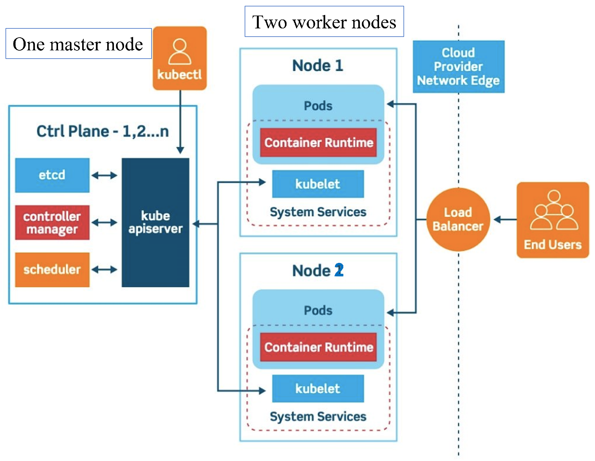
The rest of the paper is organized as follows. Section 2 presents the architecture, features, and the components of Kubernetes. Section 3 demonstrate the related work in the context of our study, such as commonly used container orchestration frameworks, load prediction methodologies and their respective principles related to our analysis, the latest custom autoscaler with obvious characteristics and excellent results, and analyzed their effectiveness and shortcomings. Section 4 is about the empirical analysis of load prediction model selection for our proposed autoscaler. Section 5 is the about the development, deployment, and evaluation of the proposed autoscaler. Conclusions and future study directions are discussed in the last section.

2. Architecture and Principles of Kubernetes

In this section, we present the details of Kubernetes including its architecture, features, and components.

2.1. Kubernetes Architecture

We observe that a Kubernetes cluster is composed of multiple nodes, divided into two groups—master nodes and worker nodes—as shown in Figure 1. The master node is the control plane of the cluster. It works with worker nodes, including the sub-modules, such as Kube APIServer, Kube Scheduler, Kube Controller Manager, ETCD, Kubectl, and other components, as shown in the right side of the figure. The worker nodes (two worker nodes are shown in the left side of the figure) are used to deploy applications in the form of containers called Pods. A worker node usually includes Kubelet, Kube-proxy, Pod, ReplicaSet, Deployment, Secret, and other components, as shown in the left side of the figure. In the context of our analysis, we present the components in Kubernetes cluster as core components, prominent components with autoscaling, prominent add-ons, and other.

2.2. Core Components

The following components are the most important and elementary components for maintaining the operation of K8s, they are Pod, ReplicaSet, Deployment, and Services, which are mainly responsible for the execution of containers, managing applications, and communication.

2.2.1. Pod

The Pod is the smallest object that developers can configure in the K8s cluster, which can run more than one container. Each container within the Pod shares the same network and K8s assigns different IP addresses for each Pod to avoid port conflicts. Generally, Pod is scheduled or managed by ReplicaSet or Deployment. Notably, we can also create a standalone Pod for testing an application. For example, we can run/deploy a Pod with an nginx image (creating a single instance of nginx application), as shown in the Listing 1.

Listing 1. Creating a standalone Pod (running an nginx server).

kubectl run nginx --image=nginx

2.2.2. ReplicaSet

ReplicaSet (RS) is a sub-component of Deployment, which provide functions such as label and selector. The label is used for marking specified Pods, and selectors help RS identify and monitor specified Pods in a myriad of Pods. Typically, ReplicaSet helps assist Deployment in managing and maintaining Pods as shown in Figure 2.

2.2.3. Deployment

Compared with ReplicaSet, Deployment comes with more features and functions, so in the real environment, developers choose Deployment to manage ReplicaSet and Pods. One of the main functions of Deployment is a rolling update, while applications in Pods need to be updated, every update can be recorded in the system, so if somehow the new version is unstable, developers can roll back to any specified version in the record. Moreover, managing ReplicaSet and Pods, and performing rolling updates, Deployments are prominently used for scaling applications. First, we see how we can run/deploy a single instance (single Pod) of an application, e.g., an nginx server, as shown in the Listing 2.

Listing 2. Creating a Deployment (running a single instance of an nginx Pod).

kubectl create deployment nginx --image=nginx

The difference of running an application with Pod and Deployment is that we can easily scale an application with the help of Deployment but not with Pod. For example (refer to the Listing 3).

Listing 3. Scaling an nginx application with the help of Deployment (running 4 instances).

kubectl scale deployments/nginx --replicas=4

Now, it can run/deploy four instances of an nginx server. At anytime we can freely increase or decrease the number of instances by changing the values of replicas parameters. Especially, we can also perform rolling update or roll back an update freely with the Deployment, as shown in the Listing 4.

Listing 4. Rolling update and rolling back of an nginx application with the Deployment.

kubectl set image deployments/nginx nginx=nginx:v3 #rolling update by v3

kubectl rollout undo deployments/nginx # rolling back to previous state

2.2.4. Services

The main function of Services (SVC) in K8s is communication. Some SVCs are responsible for connecting the internal components of the cluster, and some are responsible for the communication between the cluster and the clients. There are three types of services, such as NodePort, ClusterIP, and LoadBalancer which are as self-explanatory as their titles.

2.3. Prominent Components with Autoscaling

In this subsection, we introduce a set of three prominent components related to autoscaling activities.

2.3.1. Horizontal Pod Autoscaler (HPA)

HPA [33] is a relatively common and well-functioning reactive autoscaling strategy in K8s. HPA can manage the Deployment component to control the number of Pod counts by using the CPU utilization as a threshold, so as to achieve the purpose of autoscaling, which is shown in Figure 3. For example (refer to the Listing 5).

Listing 5. Autoscaling of an nginx application with the help of HPA.

kubectl autoscale deployment nginx --cpu-percent=70 --min=1 --max=10

In this instance, it creates an HPA for the Deployment nginx, with target CPU utilization set to 70% and the number of replicas lies between min value 1 and max value 10, which are user-defined. In detail, herein, it is to maintain an average CPU utilization limit across all Pods of the Deployment nginx to 70%, which is monitored and controlled by HPA. Notably, the limit value is user-defined that we can say desiredMetricValue as mentioned in the Expression (1) for computing the desired number of replicas if the CPU utilization exceeds the limit, which is 70% herein. If it exceeds the limit, then a new replica/Pod is deployed automatically, especially by a factor as shown in the Expression (1). Similarly, if the average CPU utilization across the Pods goes down below the limit, then the deployed replicas/Pods are shut down gradually (automatically) while maintaining the minimum number of replicas that helps optimize the resource consumption by balancing/capping the average CPU utilization within the limit. Notably, the basic algorithm for increasing or decreasing the number of replica/Pods of a particular (deployed) application is shown in the Expression (1).

$$desiredReplicas=⌈currentReplicas\times \frac{currentMetricValue}{desiredMetricValue}⌉$$

(1)

where currentReplicas denotes the number of Pods/replicas deployed currently for a particular application, and desiredReplicas denotes the number of Pods/replicas required to deploy for that application. On the other hand, as stated earlier, desiredMetricValue is the average resource utilization limit across all Pods deployed by a Deployment that is controlled by a HPA. On the other hand, the currentMetricValue is the current average resource usage which is computed by taking the average of the given metric across all Pods in the HPA’s scale target. Notably, we can use the command shown in the Listing 6 to obtain the resource usage data across the Pods, even we can filter the Pods with our specific requirement. Notably, HPA obtains utilization metric from a cluster-level component called Metrics Server [34] (this is demonstrated in the Section 2.4.1).

Listing 6. Getting/Fetching resource usage data across the Pods.

kubectl top pod

Now, we see how the desiredReplicas are computed/triggered with the resource utilization. Notably, we can track the resource utilization and the new replica/Pod deployment with the increase/decrease in resource utilization, as shown in the Listing 7.

Listing 7. Tracking of resource utilization and new replica/Pod deployment with the increase/decrease in resource utilization.

kubectl get hpa nginx

## Then we can observe the following log:

NAME       REFERENCE      TARGET    MINPODS    MAXPODS    REPLICAS    AGE

nginx     Deployment/nginx/scale   305% /70%    1         10         5         5m

Notably, to passively triggering scaling after reaching the threshold, HPA also periodically queries resource utilization to adjust the number of copies in the Deployment and RS. Last but not least, HPA supports richer scaling strategies, which can be specified in the behavior section of the spec, such as setting the time of stabilization window when scaling down and how many percents of the current replicas to be scaled down in a fixed time window. Apart from monitoring CPU utilization, HPA can also monitor custom metrics as thresholds by using interfaces defined by other programs. Notably a detailed experimental analysis is presented in Section 5.1.

2.3.2. Vertical Pod Autoscaler (VPA)

The aforementioned HPA is scaled by managing the number of Pods, while the Vertical Pod Autoscaler (VPA) [35] is scaled by reasonably allocating the CPU and memory of each Pod. Its biggest advantage is to request resources on demand or schedule the Pod to the appropriate node, which greatly improves the service efficiency of the cluster. However, compared with HPA, K8s open-source VPA is not mature enough and is in the experimental stage.

2.3.3. Cluster Autoscaler (CA)

Unlike VPA or HPA, which focus on Pod scaling, Cluster Autoscaler (CA) [36] is a component that scales the whole K8s cluster, which can automatically adjust the nodes dynamically to ensure all of the Pods can be allocated enough resources and delete nodes with low resource utilization.

2.4. Prominent Add-Ons

In this section, we introduce the prominent add-ons required for our analysis.

2.4.1. Metrics Server

Metrics Server (Metrics Server https://github.com/kubernetes-sigs/metrics-server, accessed on 10 January 2023) [34] is a cluster-level component. It periodically fetches metrics from the kubelet service through the Resource Metrics API that provides resource metrics for Pods and nodes. With this API, the metrics server can monitor metrics for HPA. In particular, Metrics Server collects resource usage metrics and passes them to K8s and is finally used by HPA for taking autoscaling decisions. However, the Metric server only records the latest value of each metric. If users need access to historical data, they need to use a third-party monitoring system or record historical metrics by themselves.

2.4.2. Prometheus

Prometheus (Prometheus https://prometheus.io/, accessed on 10 January 2023) [37] is a powerful third-party open source monitoring platform with an active developer and user community, which collects metric values in a time-series format. Moreover, it provides a visual user interface and flexible query language for users to quickly and easily obtain the target metrics.

3. Related Work

In this section, we begin with presenting a set of container orchestration frameworks while highlighting the merits and limitations of Kubernetes comparing with them. We then present the prominently used load prediction methodologies that can be integrated in our custom pod autoscaler toward predicting the load in advance for optimal scaling in Kubernetes. Then, we perform a literature review of customized proactive autoscaling strategies that have been applied to Kubernetes.

3.1. Kubernetes vs. Other Container Orchestration Frameworks

We observe that different container orchestration frameworks are developed to meet the various market needs. For detailed discussion, we go with the two easily distinguishable categories of frameworks. The first category includes fully-managed, paid, closed-source, easy deployable and manageable frameworks, such as Amazon Elastic Container Service (Amazon ECS) [12,38], Amazon Elastic Container Service for Kubernetes (EKS) [16] Google Kubernetes Engine (GKE) [16], Microsoft Azure Kubernetes Service (AKS) [16], OpenShift [13,14,39], and others. The second category includes self-managed and open-source frameworks, such as Kubernetes [7,17], Mesos [8,40], Docker Swarm [9,10,41,42], Nomad [10], SaltStack [11,43,44], and many others. Although each framework has unique features that others could do not have, their limitations dissuade some potential users. Notably, fully-managed frameworks with added features come with high cost. Moreover, they are less-customizable, less flexible, and suffer from vendor lock-in issue. On the other hand, even though open-source frameworks have a steep learning curve and have a complex setup for beginners, they are far preferred by users as they have better community services, especially Kubernetes [7,15,17,18]. We observe that among the open-source frameworks, Kubernetes is the best choice. Even compared with fully-managed services, Kubernetes is the clear winner [15,16,18,45].

Specifically, we observe comparative analyses of container orchestration frameworks in the research works [15,16] and find that Kubernetes wins the race by a fair margin (for this, we do not repeat the same analysis herein, simply inferring their analysis). Specifically, in the studies [15,16], the comparative analysis is shown among Kubernetes, Mesos, Docker Swarm, Nomad, and the fully-managed frameworks except SaltStack, while comparing with SaltStack, we see that Kubernetes is superior to SaltStack [11,43,44]. In particular, we observe that Kubernetes caters better to business needs than SaltStack. Moreover, Kubernetes is a better choice than SaltStack with quality metrics, feature updates, and other evaluation criteria [11,43,44]. Notably, Kubernetes is easier to use, as stated earlier, while the saving grace of SaltStack is that it is easier to set up, manage, and control. We also would like to state that the lack of documentation and recent research works for SaltStack results in increased complexity of usage (notably, we have checked out out the official documentation of SaltStack, https://docs.saltproject.io/en/latest/contents.html (accessed on 10 May 2023)). Specifically, Kubernetes is the dominant across the containerized application domains, such as Cloud Computing, Serverless Computing, Edge Computing, and many more. Notably, the authors in [15,46] show that Kubernetes can help stabilize the Information Technology (IT) administration and Serverless Computing efficiently, i.e., it helps stabilize the containerized applications and systems. Čilić et al. [45] analyze the performance of container orchestration frameworks for Edge Computing. Their analysis shows that Kubernetes and its derivatives are highly efficient in container orchestration across the resources of edge network compared with other orchestration frameworks.

We also observe that orchestration with Kubernetes helps optimize the Quality of Service (QoS), for example Carrión et al. [18] analyses the principles of Kubernetes scheduler in assigning physical resources to containers while optimizing QoS, such as response time, energy consumption, resource utilization, and other things. It also highlights the gaps in scheduling and concludes with future research directions to address the same.

All in all, Kubernetes has become the the de facto standard for simplifying the efficient deployment of containerized applications [7,15,17,18], so in this paper, our subject of study is Kubernetes.

3.2. Literature Review: Load Prediction Methodology

We find that the prediction results of traditional statistical analysis model [47,48] (such as ARIMA) are no longer comparable to the results predicted by the current popular deep learning models [49,50]: Long Short Term Memory (LSTM) model and the derivatives of LSTM. In this section, we demonstrate the prominent load prediction methodologies which we use in our analysis.

3.2.1. ARIMA

The Autoregressive Integrated Moving Average (ARIMA) is a classic statistical model. This model prompts to predict the potential future trends based on previous data, which has been widely used in forecasting financial trends [51] and epidemic trend [52]. As such, the time series predict result $\widehat{y_t}$ calculated based on the underlying formulation:

$$\widehat{y_t}=\mu +\sum _{i=1}^p{\varphi }_i\ast y_{t-i}+\sum _{j=1}^q{\theta }_j\ast e_{t-j}$$

(2)

In the formula, $\mu$ is a constant representing the mean of the sequence $y_t$, $y_{t-i}$ is the past ith value, and $e_{t-j}$ is past jth prediction error; ${\varphi }_i$ and ${\theta }_j$ correspond to the coefficients of autoregressive model and moving average model, respectively. The premise of using the ARIMA model for prediction is that the time series data is stationarity or stationarity after d order differencing. Therefore, the user must analyze the time series in advance and adjust the appropriate p, d, and q parameters.

3.2.2. LSTM

Before introducing the LSTM model [53], it is still necessary to introduce the Recurrent Neural Network (RNN) [54]. RNN is a deep learning model dedicated to processing sequence data or contextual data, which has been widely used to deal with sequence prediction [55], speech recognition [56], and text generation [57] tasks. However, the cell structure of RNN is too simple, which makes it easy to cause the gradient to disappear, so it is only suitable for short-term memory.

Compared with RNN, LSTM has one more hidden transmission state, and it has been added from one neural network layer to four in a single cell. The newly added neural network layer has a forgetting gate layer that controls whether to discard the previous information, an input gate layer, and a remembering gate that determines what new information is added to the cell state, which supports LSTM to learn information that has a long-term dependency, i.e., long term time series data.

3.2.3. BiLSTM

From the above RNN and LSTM models, it can be concluded that these models take into account the influence of the former text of the data on the following text. However, in actual situations, the latter part of the data also has a certain relationship with the former text. For instance, in English grammar, place related nouns are usually preceded by prepositions similar to “at” or “in”. Therefore, it is available that by inferring the previous information through the latter information, then combined with the results obtained by the forward derivation, we can obtain a more comprehensive speculation result. The example is the general idea of the Bi-directional Long Short-Term Memory (BiLSTM) model. Notably, based on the LSTM model, it derives the data forward and backward, and then concatenates the final vector to achieve the desired result. In this paper, we apply the model to the load prediction task.

3.2.4. GRU

The Gated Recurrent Unit (GRU) model [58] is also a derivative model of the LSTM model, which has a simpler network structure than the LSTM model. GRU can save computational cost by reducing the parameters that need to be learned in structure, while it can also achieve the same performance as LSTM.

$$z_t=\sigma (W_z·[h_{t-1},x_t])$$

(3)

$$r_t=\sigma (W_r·[h_{t-1},x_t])$$

(4)

$${\tilde{h}}_t=tanh(W·[r_t\ast h_{t-1},x_t])$$

(5)

$$h_t=(1-z_t)\ast h_{t-1}+z_t\ast {\tilde{h}}_t$$

(6)

3.2.5. Evaluation Metrics of Load Prediction Methodologies

Notably, in this paper, we analyze all the aforementioned methodologies as discussed in Section 4 and finally select the best one for the autoscaling task. To reasonably evaluate the results of model prediction and pick the best one, we present a set of standard evaluation metrics which are commonly used in time series forecasting, as follows:

• Mean squared error (MSE): It is the mean of the sum of squares of the errors between the true value and predicted value; we use it as a loss function to train our models.
• Root mean squared error (RMSE): It is the arithmetic square root of MSE, which focus on judging the prediction error.
• Mean absolute error (MAE): It is the mean of the absolute values of the errors between the true and predicted values.
• R-Squared ($R^2$): It is the square of the coefficients of multiple correlations between the actual values and predicted values. Notably, the closer $R^2$ is to 1, the better the model fits in general.

3.3. Literature Review: Customized Autoscaling in Kubernetes

In this section, we present the customized autoscaling strategies applied to K8s.

3.3.1. BiLSTM Based Autoscaling

As Deep Learning (DL) becomes popular, scholars have begun to try to implement deep learning models to customize autoscale. We observe that the authors in [26] propose a proactive scaling architecture based on BiLSTM. The process of scaling can be roughly summarized into two parts. The first part is the analysis phase, which applied the BiLSTM model to predict the upcoming HTTP workload. Then, the second part is the planning phase where the adaptation manager adjusts the number of Pods required according to the predicted traffic from the previous part. To evaluate the effectiveness of their proposed Proactive Custom Autoscaler (PCA), the authors used the NASA dataset from the NASA web server and perform two sets of experiments.

In the first experiment, the author chose Root Mean Square Error (RMSE) and prediction speed as the main evaluation methods. In addition to using the BiLSTM model, the famous ARIMA model is also used for comparison and testing the results of predicting one step and five steps, respectively. Judging from the results in

Table 1. Experimental results on NASA dataset.

Model Type	ARIMA	BiLSTM	ARIMA	BiLSTM
	1 Step	1 Step	5 Steps	5 Steps
MSE	196.288	183.642	237.604	207.313
RMSE	14.010	13.551	15.414	14.39
MAE	10.572	10.280	11.628	10.592
$R^2$	0.692	0.712	0.628	0.675
Prediction-speed (ms)	2299	4.3	2488	45.1

The best values are marked as bold.

, BiLSTM is better than ARIMA in terms of prediction accuracy and speed, since the MSE, RMSE, and MAE are lower and the $R^2$ is larger; therefore, it has a very high prediction speed.

The second set of experiments is to take part of the continuous data of the NASA dataset as input, to test and compare Proactive PCA with BiLSTM and HPA with traditional K8s. Figure 4 illustrates that the number of Pods and resources scheduled by PCA fits well with the actual load. Compared with PCA, the shortcomings of allocation by HPA are obvious. First of all, HPA allocates many more resources than are needed, resulting in many resources not being used. Second, due to HPA’s cooldown mechanism, there will be a significant delay every time a scaling operation is triggered, which exacerbates the problem of resource waste. Notably, we learn their evaluation method to measure the prediction model; the autoscaler helps us better analyze our experimental results.

Summary: It is all good that the authors have achieved better results with BiLSTM compared with ARIMA. Notably, it is usual that prediction with BiLSTM should be better than with ARIMA since it autoregressive model. However, the issue with BiLSTM is that BiLSTM does not suit the time sequence data well. We can not have the future time sequence data, e.g., stock price tomorrow or one month later, as such we can not process the time sequence data bidirectionally well. In particular, BiLSTM suits well with text data, e.g., Named Entity Recognition (e.g., General Motors (General Motors, USA, https://www.gm.com/, accessed on 20 March 2023) manufactures cars and trucks), Next Sentence/Word Prediction (e.g., I am        very hungry, I could eat half a pig.). For this, in our analysis, we add other two deep learning based time sequence analyzing models, such as LSTM and GRU.

3.3.2. HPA+

HPA+, a proactive scaling engine is proposed by Toka et al. [27]. The difference with the aforementioned scheme is that in addition to the LSTM model, Auto-regressive (AR), Hierarchical Temporal Memory (HTM), and Reinforcement Learning (RL)-based prediction models are also integrated for comprehensive prediction. Notably, the authors carried the experimental analysis with Markov-modulated Poisson Process (MMPP) [59] trace-driven simulation. The experimental analysis shows that the discrete-time HPA performs worst in prediction, because this is the inherent drawback of reactive scaling. On the other hand, the AR model and LSTM model have the best performance. Compared with other models, HTM and RL prediction models perform poorly. Notably, HPA+ analyses the prediction and with time the best prediction model is triggered, thereby the proactive scaling is operated. In proactive scaling, we find that HPA+ performs better compared with the native HPA in enhancing the quality of service. However, it results in excess of Pod/resource usage. Notably, the authors employ a set of policies, such as Conservative, Normal, and Best Effort to minimize the resource usage while meeting user requests respectfully.

Summary: HPA+ autoscaling engine proposes a nearly perfect solution, which is to implement a variety of different prediction models to complement each other. However, we believe that even if a good precision of prediction has been attained, a tremendous amount of computing resources are needed for forecasting.

3.3.3. Holt–Winters Exponential Smoothing on K8s VPA

The previous two research works have used various methods that modify the scaling decision in a custom autoscaler to improve the performance of HPA. On the other hand, this article [28] implements the Holt–Winters (HW) exponential smoothing algorithm and LSTM model to optimize VPA.

Before introducing the HW method, we introduce the Exponential Smoothing method, since the HW method is built on top of it. Exponential Smoothing method is a time series algorithm that takes a weight based on the comparison between the most recent observation and the previous average. One of the most used methods of exponential smoothing methods is Simple Exponential Smoothing, which is very suitable for forecasting data that does not have a fixed pattern or seasonality. Contrast to Simple Exponential Smoothing, HW method adds two more components in order to extract the seasonality of the data, so it is also called Triple Exponential Smoothing method.

To test the performance of Holt–Winters method, the author collected historical data that present either seasonal and irregular on Alibaba containers. Similarly, the author also implemented the LSTM model to join the experiment for comparison. The experiment results shows that the HW model is well suited for seasonal requests. However, when the CPU request behaves irregularly, the HW model performs poorly.

Summary: As per the analysis in this subsection, HW model is to optimize VPA (Vertical Pod Autoscaler), to scale by reasonably allocating the CPU and memory of each Pod. On the one hand, in this paper, our objective is optimize the HPA. On the other hand, we observe that HW model works well for seasonal data, but performs poorly when the data behaves irregularly. To address this, the LSTM or GRU model suit well, no matter whether the data is seasonal or irregular, they can show better performance, which indicates that the LSTM or GRU has better robustness.

3.3.4. LIBRA Autoscaling

Currently, native HPA and VPA in K8s cannot run simultaneously that monitors CPU and memory metrics, in order to maximize their respective performance, this article proposed an autoscaler called LIBRA [60] running on the top of K8s, which mix the advantages of horizontal and vertical scaling.

To test the performance of LIBRA, the author used hey—HTTP load generator (https://github.com/rakyll/hey, accessed on 10 January 2023) to produce a request with the concurrency level of 50 as 10 min long measurements. The native K8s VPA cannot work with HPA, which uses CPU utilization as an indicator, and LIBRA combines both the HPA and VPA; therefore, on the premise of fairness the author only compares the gains of these two methods. For the K8s HPA, the threshold was set to 90% and the service scaled up to four Pods. After reaching the max number of Pods, it can serve about 150 RPS (Request Per Second). As for LIBRA, the threshold also was set to 90% and LIBRA set the CPU limit of the serving Pod to 15%. Compared to HPA, it can provide 100 more RPS, and the scaled maximum number of Pods is doubled.

LIBRA can provide faster service than HPA from the perspective of threads: Single-threaded applications can simply increase the resource pool through horizontal scaling, while multi-threaded applications can effectively use the resources of multiple CPU cores through vertical scaling.

Summary: We observe that LIBRA can combine the HPA and VPA to provide more service capacity compared to the original HPA. However, as stated earlier, K8s open-source VPA is not mature enough and is in the experimental stage, so we solely focus on horizontal autoscaling. Another point is that VPA is mostly useful for resource allocation on demand or for scheduling a Pod to an appropriate node. Conversely, in this paper, we focus on satisfying the demand of multiple myriad requests of an application synchronously and in parallel with greater isolation.

3.3.5. Discussion

In this section, we demonstrate a set of autoscaling methods employed to K8s, such as BiLSTM based Autoscaling, HPA+, and Holt–Winters Exponential Smoothing on K8s VPA, and LIBRA Autoscaling. We observe that their working principles vary from method to method and also to validate their effectiveness; different sets of datasets and different sets of evaluation metrics are used across the methods. Thereby, it is not reasonable to show a comparative analysis among them. Therefore, we briefly present a summary of each method stating the merits and limitations.

4. Proposed Autoscaler: Load Prediction Model Selection

In this section, we delve into the selection of a load prediction model, which is the first step of the three steps of our customized autoscaling scheme. First, it is about the dataset and selection of the appropriate prediction objects. Thereafter, the performance evaluation of each prediction model. We use Tensorflow 2 to analyze our work.

4.1. Dataset

The dataset of this experiment uses historical data called clusterdata-2011-2 collected from the Borg [7] cluster, which collected data from 12.5k machines for 29 days. In addition to being used for load forecasting [61], this dataset is also used for research in other fields such as Mobile Edge Computing [62] and Resource Reservation [30]. Notably, the cluster data size is 41 GB and is divided into six types, as follows:

• job_events
• machine_attributes
• machine_events
• task_constrains
• task_events
• task_usage

The main dataset among them used in the experiment is task_usage, which contains a large amount of detailed data such as the measurement period, machine id, CPU usage rate, and memory usage rate as a csv file.

4.2. Preprocessing

After extracting the dataset, we can observe that the dataset (Figure 5) has a 300 s measurement period having the average CPU rate, memory rate, and machine IDs. Next, we randomly sample data from 100 machines of the raw dataset, where each row records the CPU rate and memory at 8352-time points. Finally, we save the processed data in a Pickle file (pkl format) to simulate the CPU load and memory load for training the network model.

Since we can only target one type of load as a scaling metric in K8s, we need to confirm whether different loads would affect each other, so we choose Pearson correlation coefficient [63] to measure the correlation between loads. We calculate the correlation coefficient value as 0.208 from a single randomly selected machine and conclude a weak positive correlation between CPU rate and Memory rate. Therefore, we can use CPU and memory as two datasets to perform load prediction separately.

4.3. Network Model Configuration

We train and compare LSTM, BiLSTM, and GRU models as experimental objects. Notably,

Table 2. Configuration of each model.

Parameter	LSTM	BiLSTM	GRU
hidden unit	50	100	50
Activation function	relu	relu	relu
batch size	512	512	512
Epochs	200	200	200
Optimizer	adam	adam	adam
Loss function	MSE	MSE	MSE

list the default parameters of the models. As we know, data science is about performing experiments, so we come with these parameters after several trials.

4.4. Experiment Results

In this section, we show the experimental analysis of the statistical analysis model, ARIMA, and the three deep learning models, LSTM, BiLSTM, and GRU. Notably, we assume the ARIMA model as the baseline model. For the statistical analysis model, we analyzed the original sequence in clusterdata-2011-2 and chose this sequence as the training set. For the deep learning models, we randomly select one sequence in the dataset as the training set and perform multi-step training and save the model of each prediction step. Then we randomly selected 10 sequences different from the training set as the common test set for each model and assessed the test results of each model through evaluation metrics. Notably, we determined ARIMA parameters (p, d, q) as (3, 1, 2). Then, we selected 10 sequences randomly as the test set and the test results were recorded for further analysis. The prediction result of the ARIMA model is shown in Figure 6 and detailed measurement data are shown in

Table 3. Experiment result on Clusterdata-2011-2.

Model	ARIMA	LSTM	BiLSTM	GRU
Best Step Size	-	47 Step	45 Step	24 Step
MSE	0.00197	0.00195	0.00195	0.00194
RMSE	0.04429	0.04367	0.04369	0.04360
MAE	0.03202	0.03274	0.03101	0.03057
Training Time (s)	-	1.44	2.41	0.75
Prediction Time (s)	4.1441	0.0661	0.0665	0.0651

for comparison with other models.

For deep learning models, we used the CPU usage rate of one of the 100 randomly selected machines as the training set to train the models of LSTM, BiLSTM, and GRU with prediction steps from 1 to 50, respectively. From the loss graphs in Figure 7, Figure 8 and Figure 9, we observe that the convergence speed of the three models is very fast that need only 3 to 5 epochs to reach the lowest loss value. Therefore, in the next task, the number of epochs can be reduced to save training time. On the validation loss graphs, we can see that with the epoch increases, the loss of LSTM generates a small number of fluctuations; this fluctuation is more obvious in the BiLSTM model, while the GRU model has the most stable performance.

Subsequently, we input the data of 10 machines that are not repeated at random into the trained model for testing. The predicted and true values of the two models are obtained. Figure 10, Figure 11 and Figure 12 show the predicted and true values of each model; we can observe that LSTM model and BiLSTM has almost the same performance, while the GRU model has better performance in predicting load peaks. We can observe that it is difficult to distinguish the LSTM and BiLSTM model by the aforementioned figures.

To further compare the performance among the three models, we use the MSE evaluation metric as the model’s prediction accuracy. We take the average of the MSE value obtained from each step test of every 10 machines to eliminate abnormal values. This method produces the MSE comparison chart as shown in Figure 13. From the figure, we can say that the MSE decreases as the prediction step increases. From the data distribution point of view, the distribution of GRU is relatively stable and the prediction accuracy is better than other models, then LSTM followed by BiLSTM. The best results of LSTM, BiLSTM, and GRU models are 0.00195 in the 47th step, 0.00195 in the 45th step and 0.00194 in the 24th step, respectively.

In addition, we also added the model’s training time and prediction time to the reference indicators. Figure 14 and Figure 15 compare the training time and prediction time of each step of the three models, respectively. As the prediction step size increases from 1 to 50, the training time and prediction time required for the three models are becoming longer in general. From the perspective of training time, the overall training time and growth speed of the GRU model are slightly lower than that of the LSTM model because of its simpler network structure. As the prediction step size increases, the BiLSTM model takes almost twice the training time of the GRU and LSTM models. From the perspective of prediction time, the prediction times for all three models are distributed from 0.0645 s to 0.0675 s. From the fitted straight line we can conclude that the prediction time of the GRU and LSTM models is almost the same, and the prediction time of BiLSTM is slightly higher than the previous two models.

Since the above experimental results are all statistics in Table 3, we can intuitively compare the experimental results of each model. From the perspective of prediction accuracy, the accuracy of each deep learning model is slightly better than that of traditional prediction models. In terms of average prediction time, the ARIMA model takes an average of 4.1441 s per prediction step, while each deep learning model takes around 0.06 s, which shows the result of the deep learning model is much better than traditional forecasting models. Therefore, deep learning models perform better than traditional forecasting models in terms of prediction accuracy and prediction time. Among them, the GRU is the best model in all aspects, and we encapsulate the model into the prediction logic for further experiments.

We know that the performance of GRU and LSTM does not vary a lot [64,65]. As we observe that except the training time, their performance is closely aligned. However, we know that GRU more simplified with less gates and less parameters than LSTM that makes it faster and simpler, however sometimes less adaptable and less efficient. On the other hand, since, LSTM has more logic gates and more parameters than GRU, it can add more flexibility and more expressiveness while incurring more computational cost, training time, and risk of overfitting. In fact, both the LSTM and GRU are alternatively used in time sequence data analysis and they perform more or less equally with respect to the nature of data [64,65].

5. Proposed Autoscaler: Deployment and Experimental Analysis

To be able to simulate the real K8s cluster for experiments under limited machines, we decide to build a cluster by creating virtual machines in local environment having one master node, and two worker nodes. Notably, we can add or remove nodes freely.

Here are the specific configurations:

• Windows10 VirtualBox;
• Virtual machines: Ubuntu 16.04 LTS;
• Kubernetes installation source: Kubeadm (Creating a K8s cluster with Kubeadm https://kubernetes.io/docs/setup/production-environment/tools/kubeadm/create-cluster-kubeadm/, accessed on 10 January 2023);
• Kubernetes version: 1.20;
• Docker version: 19.03.

5.1. Reactive (Default) Autoscaling in K8s (HPA in K8s)

After deploying the K8s cluster according to the above configuration, we created a simple yaml file and named it nginx-hpa.yaml for testing. This yaml file contains the configuration of two components, one is Deployment that is responsible for managing a Pod with a Docker image, e.g., an nginx [66] image. To ensure HPA works normally the CPU resource is also configured for the containers in the cluster that running the application, limit, and request are 500 m and 50 m, respectively. The other component is the Service that exposes the service for external access. Next, we run the following command to apply the yaml configuration, as shown in the Listing 8.

Listing 8. Creation of a HPA having the Deployment for an nginx server.

kubectl apply -f nginx-hpa.yaml

Then waiting for the Deployment and Service to be created and become “Running” status, we can successfully access the deployed nginx network service by accessing the IP address of any worker node and corresponding port number. Now, we apply HPA by entering the command, as shown in the Listing 9.

Listing 9. Autoscaling of nginx HPA limiting the CPU usage to $10\%$ having the replica Pods between 1 and 10.

kubectl autoscale deployment nginx-hpa --cpu-percent=10 --min=1 --max=10

We set the upper limit of CPU usage to 10% to quickly trigger scaling and set the minimum and maximum number of Pods for each replica to 1 and 10, respectively, to represent the scale of scaling. Finally, we create a load generator image by executing the command, as shown in the Listing 10 to continuously generate requests for worker nodes to access the nginx page we just created to stress test the cluster.

Listing 10. Load generator for accessing the ngnix server deployed by the nginx HPA.

kubectl run -i --tty load-generator --rm --image=busybox

--restart=Never -- /bin/sh -c ⸌⸌while true;

do wget -q -O- http://192.168.56.110:30003;

wget -q -O- http://192.168.56.111:30003; done"

We run the command, as shown in the Listing 11 to observe the actual running state of HPA.

Listing 11. Getting/Fetching data about the HPA.

kubectl get hpa

Notably, we trace the running state of HPA, when the stress test starts at “8m” (at the 8th minute). We observe that HPA did not detect the surge of requests and did not scale the replicas respectfully until about 50s have passed. One more important point to note is that when the stress test ends at “9m” (at 9th minute), HPA takes more than 1 min to perform scale down. The log shown in Figure 16 illustrates that for a sudden increase in requests, there is still a considerable delay in HPA response.

5.2. Proactive Autoscaling in K8s (CPA in K8s)

In this section, we demonstrate the CPA framework, our CPA, and the specific packaging and deployment process of our CPA.

5.2.1. Introduction to CPA Framework

Custom Pod Autoscaler (CPA) framework [31] is a customizable K8s autoscaler developed by the DigitalOcean team (DigitalOcean https://www.digitalocean.com/, accessed on 10 January 2023). It runs in a set of CPA frameworks written in the Go programming language. This framework abstracts the complex interaction process between CPA and K8s, allowing developers to use any language to write scaling logic, which has better scalability and easier management than K8s native HPA.

CPA frameworks provides developers with two stages for customizing the scaling logic: metrics gathering and evaluation. The job of the first stage metrics gathering is mainly used to collect metrics in K8s, and pass the user-defined metrics to be collected to the next stage in json format. It also works as an API that can be called to check the metrics usage of the target container or application at the current moment. The job of the evaluation stage is to pass the collected metrics as input to the scaling logic defined by the developer to decide whether to scale up or scale down to the target number of replicas.

The custom pod autoscaler operator (Custom Pod Autoscaler Operator https://github.com/jthomperoo/custom-pod-autoscaler-operator, accessed on 10 January 2023) [67] is a framework of CPA. It is an operator that takes the responsibility of creating a developer-defined CPA in the cluster as shown in Figure 17. Especially, deploying CPA operator in the cluster is also a prerequisite for deploying CPA.

5.2.2. Workflow of Our Custom Pod Autoscaler

In this section, we show step by step how to write custom autoscaling logic, encapsulate the logic into a CPA image, and finally deploy proactive autoscaler to the cluster to achieve custom autoscaling.

The workflow of the two stages in CPA is shown in Figure 18, such as Metric Gatherer and Evaluator. Herein, we define metric.py as a Metric Gatherer and define evaluate.py as an Evaluator that predicts load and computes replicas:

1.

Read target metric and information from the K8s Metrics Server.

2(a).

Convert the current number of replicas and CPU usage to JSON format and pass it to the Evaluator.

2(b).

Collect and update the historical time sequence locally into the database.

3.

Load the deep learning model and read historical time sequence to Evaluator for predicting and calculating the replicas.

4.

Assign the target number of replicas calculated by Evaluator.

Next, we introduce the internal implementation logic of the Metric Gatherer and Evaluator in detail through two flowcharts as shown in Figure 19 and Figure 20.

The main job of the Metric Gatherer (Figure 19) is to collect information about the target application. In particular, it collects the Pod information running by the target application from the K8s metrics server, then extracts the current number of copies $Cur\_r$ and the CPU usage of each Pod. Next, the total CPU usage $Tot\_u$ is obtained by summing the CPU usage of each target Pod, and then the average CPU usage $Avg\_u$ is obtained through $Tot\_u$. After that, it saves the current $Av{g}_u$ to the database and updates the historical time series $Seq\left[\right]$, and finally converts $Cur\_r$ and $Avg\_u$ into JSON format and passes it to the Evaluator.

The Evaluator (Figure 20) is primarily responsible for executing the scaling logic. First, it receives the $Cur\_r$ and $Avg\_u$ passed from the Metrics Gatherer and reads the corresponding values from the JSON file, and then reads the historical time series $Seq\left[\right]$ and the pre-trained model $Pre\_model$ from the database. Initialize the target CPU usage threshold $Tar\_ut$ and the target number of replicas $Tar\_r$ to 50 and 0, respectively. Then judge whether the historical sequence length $Seq\_len$ is greater than the input size $Inp\_size$ required by the model. If so, $Seq\left[\right]$ is passed into $Pre\_model$ as input to predict the average CPU usage $Pre\_u$ for the next step (next period of time), and then execute the HPA algorithm to calculate the corresponding $Tar\_r$. If the time sequence does not meet the model input length, it then simply executes the original HPA logic that calculates the corresponding $Tar\_r$ through $Cur\_r$ and $Avg\_u$. Finally, it converts $Tar\_r$ into JSON format and sends it to Deployment to execute the autoscaling strategy to the specified number of replicas.

5.2.3. Development and Shipment of CPA Image

In this section, we show the file structure and configuration required to build a CPA image. Notably, we have uploaded the CPA image building workflow to Github (CPA Image https://github.com/vikinglion/Autoscaler/tree/main/k8s-metrics-cpu, accessed on 20 January 2023), which also includes the configuration files for HPA and other files to carry out the experimental analysis as discussed in the later part of this paper. The file structure for the CPA image is, as shown in the Listing 12.

Listing 12. File structure for the CPA image.

k8s-metrics-cpu

-- GRU_Model_24

-- config.yaml

-- cpa.yaml

-- Dockerfile

-- metric.py

-- evaluate.py

-- requirements.txt

The workflow of metric.py and evaluate.py has been explained in detail in the previous subsection. We set the CPA configuration through config.yaml (shown in the Listing 13) for the autoscaler, which defines which scripts to run, how to call them, and a timeout for the script. We define the shell command method to drive the CPA to call the custom script and judge whether the user-defined logic is successfully called by the return value of the script. Next, we set K8s metrics server configuration to allow CPA automatically gather designated metrics such as CPU and memory. In the experiment, we set the CPU as the collection metric.

Listing 13. Configuration for the CPA image (config.yaml).

evaluate:

type: "shell"

timeout: 12500

shell:

entrypoint: "python"

command:

- "/evaluate.py"

metric:

type: "shell"

timeout: 12500

shell:

entrypoint: "python"

command:

- "/metric.py"

kubernetesMetricSpecs:

- type: Resource

resource:

name: cpu

target:

type: Utilization

requireKubernetesMetrics: true

After the configuration file is set, start to package the Dockerfile to build the CPA image. We pull in python:3.8-slim version and put the environment required by the custom script into the requirement.txt file. Finally, add the CPA configuration file config.yaml, custom scaling scripts metric.py and evaluate.py, trained model GRU_Model_24 to the environment. After that, we run the command, as shown in the Listing 14 to build a Docker image for the CPA image (Notably, the image is created in to the local repository). Due to network problems, the image cannot be directly uploaded to Docker Hub (Docker Hub https://hub.docker.com/, accessed on 10 January 2023), we push it to the public repository of Alibaba Cloud (Alibaba Cloud https://www.aliyun.com/, accessed on 10 January 2023).

Listing 14. Building a Docker image for the our custom CPA and uploading it to public repository.

docker build -t vikinglion/k8s-metrics-cpu:latest .

docker push registry.cn-hangzhou.aliyuncs.com/ vikinglion/k8s-metrics-cpu:latest

5.2.4. Deployment of CPA Image and Testing on K8s

As mentioned in the previous subsection, the prerequisite for the operation of our CPA is the successful installation of the CPA operator, so the first step is to determine the version corresponding to K8s and the operator, and then enter the command to install, as shown in the Listing 15.

Listing 15. Installation of Custom Pod Autoscaler Operator.

VERSION=v1.2.1

HELM_CHART=custom-pod-autoscaler-operator

helm install ${HELM_CHART} https://github.com/ jthomperoo/custom-pod-autoscaler-operator/

releases/download/${VERSION}/ custom-pod-autoscaler-operator-${VERSION}.tgz

Next, we focus on configuring cpa.yaml to deploy CPA, as shown in the Listing 16. First, we pull the created CPA image from the public repository of Alibaba Cloud, and then set the target application and metric in the cluster as same as the experiment in HPA. In addition, the CPA framework has also encapsulated the stabilization window mechanism; here we set it to 60 s.

Listing 16. Configuration file for deploying the CPA image while monitoring an application called php-cpa (cpa.yaml).

apiVersion: custompodautoscaler.com/v1

kind: CustomPodAutoscaler

metadata:

name: k8s-metrics-cpu

spec:

template:

spec:

containers:

- name: k8s-metrics-cpu

image: registry.cn-hangzhou.aliyuncs.com/vikinglion/k8s-metrics-cpu:latest

imagePullPolicy: IfNotPresent

scaleTargetRef:

apiVersion: apps/v1

kind: Deployment

name: php-cpa

roleRequiresMetricsServer: true

config:

- name: interval

value: "10000"

- name: downscaleStabilization

value: "60"

To generate a more stable load from the tested application, we chose the test image php-apache.yaml on the K8s official website, the application of this image defines an index.php page, and executes a for loop statement to generate CPU usage to simulate the load in the cluster. In this experiment, we copied and renamed php-apache.yaml to php-hpa.yaml and php-cpa.yaml, and deployed two identical content (two Deployments) with different names, respectively, which is used to compare the scaling effect of CPA and native HPA.

It is convenient to quickly deploy HPA through the command line; however, it is inconvenient to modify the configuration information, so we also configured hpa.yaml and the target CPU usage threshold is set to 50%, the maximum and minimum number of replicas are 20 and 1, respectively, and the stabilization window time is to 60s as in CPA. The next step is to deploy the aforementioned YAML files in the cluster. Consequently, we go in the following way, as shown in the Listing 17.

Listing 17. Deployment of HPA and CPA, and Performance analysis.

kubectl apply -f php-cpa.yaml

kubectl apply -f php-hpa.yaml

kubectl apply -f cpa.yaml

kubectl apply -f hpa.yaml

As in the previous HPA experiments, we trigger the target application to execute business logic by configuring load-generator.yaml. The working principle is to access php-cpa and php-hpa applications separately every 0.01 s through ClusterIP.

After deploying the load-generator, we captured 20 min of data to show the results. The process of scaling the number of replicas of php-cpa and php-hpa was displayed from the control interface of Prometheus (Figure 21). The blue and red lines represent the number of replicas of php-cpa and php-hpa, respectively. It can be observed from the figure that the load trend generated by the test application is relatively stable, so the autoscaling process of HPA and CPA is roughly the same with a small amount of error, which also proves that our proposed autoscaling scheme is feasible after deployed on the real K8s cluster.

6. Conclusions and Future Work

Deploying applications through cloud computing services has become the choice of most users. One of the important functions is autoscaling, which is still implemented through reactive methods to trigger scaling logic and cannot meet the needs of all users respectfully. Therefore, it is necessary to analyze specific applications and customize the corresponding scaling strategy. To this, we begin with proposing a proactive scaling scheme that is based on the GRU deep learning model to address the shortcomings of the default autoscaler, HPA. In particular, we develop a load prediction model based on GRU for the autoscaler, then based on the predicted load, our custom autoscaler scales the replicas of a deployed application to meet the user demands. Respectively, we implement our custom autoscaling scheme, deploy it to the real K8s cluster, and empirically evaluate the effectiveness of it.

The paramount advantage of our scaling scheme is that it can train the model for each metric respectfully and replace the scaling logic at any time, which has better scalability. However, there are still aspects that need to be improved in our scheme. We develop our load prediction model in terms of CPU utilization in a node. In load prediction, it would be good if we could develop the model for individual tasks; however, this would increase the training complexity. In other aspect, while testing our custom pod autoscaler, we use a load generator to trigger and drive the test application to generate CPU load in K8s. This form of test method cannot generate custom target values duly, so this is our primary problem that needs to be solved in the future. In addition, all of the prediction models are based on the supervised learning method, which relies on models that are fully trained on target metrics, so we will consider other viable strategies such as reinforcement learning or other state-of-the-art methods as alternatives.

References

1. Chiueh, S.N.T.C.; Brook, S. A survey on virtualization technologies. Rpe Rep. 2005, 142, 1–42. [Google Scholar]
2. Uhlig, R.; Neiger, G.; Rodgers, D.; Santoni, A.L.; Martins, F.C.; Anderson, A.V.; Bennett, S.M.; Kagi, A.; Leung, F.H.; Smith, L. Intel virtualization technology. Computer 2005, 38, 48–56. [Google Scholar] [CrossRef]
3. Mao, M.; Humphrey, M. A performance study on the vm startup time in the cloud. In Proceedings of the 2012 IEEE 5th International Conference on Cloud Computing, Honolulu, HI, USA, 24–29 July 2012; pp. 423–430. [Google Scholar]
4. Xavier, M.G.; Neves, M.V.; Rossi, F.D.; Ferreto, T.C.; Lange, T.; De Rose, C.A. Performance evaluation of container-based virtualization for high performance computing environments. In Proceedings of the 2013 21st Euromicro International Conference on Parallel, Distributed, and Network-Based Processing, Belfast, UK, 27 February–1 March 2013; pp. 233–240. [Google Scholar]
5. Soltesz, S.; Pötzl, H.; Fiuczynski, M.E.; Bavier, A.; Peterson, L. Container-based operating system virtualization: A scalable, high-performance alternative to hypervisors. In Proceedings of the 2nd ACM SIGOPS/EuroSys European Conference on Computer Systems 2007, Lisbon, Portugal, 21–23 March 2007; pp. 275–287. [Google Scholar]
6. Anderson, C. Docker [software engineering]. IEEE Softw. 2015, 32, 102-c3. [Google Scholar] [CrossRef]
7. Burns, B.; Grant, B.; Oppenheimer, D.; Brewer, E.; Wilkes, J. Borg, omega, and kubernetes. Queue 2016, 14, 70–93. [Google Scholar] [CrossRef] [Green Version]
8. Truyen, E.; Van Landuyt, D.; Preuveneers, D.; Lagaisse, B.; Joosen, W. A comprehensive feature comparison study of open-source container orchestration frameworks. Appl. Sci. 2019, 9, 931. [Google Scholar] [CrossRef] [Green Version]
9. Naik, N. Building a virtual system of systems using docker swarm in multiple clouds. In Proceedings of the 2016 IEEE International Symposium on Systems Engineering (ISSE), Edinburgh, UK, 3–5 October 2016; pp. 1–3. [Google Scholar]
10. Guerrero, C.; Lera, I.; Juiz, C. Resource optimization of container orchestration: A case study in multi-cloud microservices-based applications. J. Supercomput. 2018, 74, 2956–2983. [Google Scholar] [CrossRef]
11. Zadka, M.; Zadka, M. Salt Stack. In DevOps in Python: Infrastructure as Python; Apress: New York, NY, USA, 2019; pp. 121–137. [Google Scholar]
12. Acuña, P. Amazon EC2 container service. In Deploying Rails with Docker, Kubernetes and ECS; Springer: Cham, Switzerland, 2016; pp. 69–98. [Google Scholar]
13. Pousty, S.; Miller, K. Getting Started with OpenShift: A Guide for Impatient Beginners; O’Reilly Media, Inc.: Sebastopol, CA, USA, 2014. [Google Scholar]
14. Lossent, A.; Peon, A.R.; Wagner, A. PaaS for web applications with OpenShift Origin. J. Phys. Conf. Ser. 2017, 898, 082037. [Google Scholar] [CrossRef] [Green Version]
15. Mondal, S.K.; Pan, R.; Kabir, H.; Tian, T.; Dai, H.N. Kubernetes in IT administration and serverless computing: An empirical study and research challenges. J. Supercomput. 2022, 78, 2937–2987. [Google Scholar] [CrossRef]
16. Ferreira, A.P.; Sinnott, R. A performance evaluation of containers running on managed kubernetes services. In Proceedings of the 2019 IEEE International Conference on Cloud Computing Technology and Science (CloudCom), Sydney, Australia, 11–13 December 2019; pp. 199–208. [Google Scholar]
17. Sayfan, G. Mastering Kubernetes; Packt Publishing Ltd.: Birmingham, UK, 2017. [Google Scholar]
18. Carrión, C. Kubernetes scheduling: Taxonomy, ongoing issues and challenges. ACM Comput. Surv. 2022, 55, 1–37. [Google Scholar] [CrossRef]
19. Brewer, E.A. Kubernetes and the path to cloud native. In Proceedings of the 6th ACM Symposium on Cloud Computing, Kohala Coast, HI, USA, 27–29 August 2015; p. 167. [Google Scholar]
20. Vayghan, L.A.; Saied, M.A.; Toeroe, M.; Khendek, F. Deploying microservice based applications with kubernetes: Experiments and lessons learned. In Proceedings of the 2018 IEEE 11th International Conference on Cloud Computing (CLOUD), San Francisco, CA, USA, 2–7 July 2018; pp. 970–973. [Google Scholar]
21. Zhang, H.; Jiang, G.; Yoshihira, K.; Chen, H.; Saxena, A. Intelligent workload factoring for a hybrid cloud computing model. In Proceedings of the 2009 Congress on Services-I, Los Angeles, CA, USA, 6–10 July 2009; pp. 701–708. [Google Scholar]
22. Moore, L.R.; Bean, K.; Ellahi, T. Transforming reactive auto-scaling into proactive auto-scaling. In Proceedings of the 3rd International Workshop on Cloud Data and Platforms, Prague, Czech Republic, 14–17 April 2013; pp. 7–12. [Google Scholar]
23. Al-Dhuraibi, Y.; Paraiso, F.; Djarallah, N.; Merle, P. Autonomic vertical elasticity of docker containers with elasticdocker. In Proceedings of the 2017 IEEE 10th International Conference on Cloud Computing (CLOUD), Honolulu, HI, USA, 25–30 June 2017; pp. 472–479. [Google Scholar]
24. Morais, F.J.A.; Brasileiro, F.V.; Lopes, R.V.; Santos, R.A.; Satterfield, W.; Rosa, L. Autoflex: Service agnostic auto-scaling framework for iaas deployment models. In Proceedings of the 2013 13th IEEE/ACM International Symposium on Cluster, Cloud, and Grid Computing, Delft, The Netherlands, 13–16 May 2013; pp. 42–49. [Google Scholar]
25. Imdoukh, M.; Ahmad, I.; Alfailakawi, M.G. Machine learning-based auto-scaling for containerized applications. Neural Comput. Appl. 2020, 32, 9745–9760. [Google Scholar] [CrossRef]
26. Dang-Quang, N.M.; Yoo, M. Deep Learning-Based Autoscaling Using Bidirectional Long Short-Term Memory for Kubernetes. Appl. Sci. 2021, 11, 3835. [Google Scholar] [CrossRef]
27. Toka, L.; Dobreff, G.; Fodor, B.; Sonkoly, B. Machine learning-based scaling management for kubernetes edge clusters. IEEE Trans. Netw. Serv. Manag. 2021, 18, 958–972. [Google Scholar] [CrossRef]
28. Wang, T. Predictive Vertical CPU Autoscaling in Kubernetes Based on Time-Series Forecasting with Holt-Winters Exponential Smoothing and Long Short-Term Memory. 2021. Available online: http://www.diva-portal.org/smash/record.jsf?pid=diva2%3A1553841&dswid=-8736 (accessed on 10 January 2023).
29. Yan, M.; Liang, X.; Lu, Z.; Wu, J.; Zhang, W. HANSEL: Adaptive horizontal scaling of microservices using Bi-LSTM. Appl. Soft Comput. 2021, 105, 107216. [Google Scholar] [CrossRef]
30. Biran, O.; Breitgand, D.; Lorenz, D.; Masin, M.; Raichstein, E.; Weit, A.; Iyoob, I. Heterogeneous resource reservation. In Proceedings of the 2018 IEEE International Conference on Cloud Engineering (IC2E), Orlando, FL, USA, 17–20 April 2018; pp. 141–147. [Google Scholar]
31. Thompson, J. Custom Pod Autoscaler. Available online: https://github.com/jthomperoo/custom-pod-autoscaler (accessed on 6 January 2023).
32. Kubernetes Architecture and Concepts. Available online: https://platform9.com/blog/kubernetes-enterprise-chapter-2-kubernetes-architecture-concepts/ (accessed on 10 January 2023).
33. Kubernetes. How Does a HorizontalPodAutoscaler Work? Available online: https://kubernetes.io/docs/tasks/run-application/horizontal-pod-autoscale/ (accessed on 6 January 2023).
34. Kubernetes. Kubernetes Metrics Server. Available online: https://github.com/kubernetes-sigs/metrics-server/ (accessed on 6 January 2023).
35. Kubernetes. Vertical Pod Autoscaler. Available online: https://github.com/kubernetes/autoscaler/tree/master/vertical-pod-autoscaler (accessed on 6 January 2023).
36. Kubernetes. Cluster Autoscaler. Available online: https://github.com/kubernetes/autoscaler/tree/master/cluster-autoscaler (accessed on 6 January 2023).
37. Padgham, L.; Winikoff, M. Prometheus: A methodology for developing intelligent agents. In Proceedings of the International Workshop on Agent-Oriented Software Engineering, Bologna, Italy, 15 July 2002; pp. 174–185. [Google Scholar]
38. Ifrah, S. Deploying Containerized Applications with Amazon ECS. In Deploy Containers on AWS; Springer: Cham, Switzerland, 2019; pp. 83–133. [Google Scholar]
39. Aly, M.; Khomh, F.; Yacout, S. Kubernetes or openShift? Which technology best suits eclipse hono IoT deployments. In Proceedings of the 2018 IEEE 11th Conference on Service-Oriented Computing and Applications (SOCA), Paris, France, 20–22 November 2018; pp. 113–120. [Google Scholar]
40. Al Jawarneh, I.M.; Bellavista, P.; Bosi, F.; Foschini, L.; Martuscelli, G.; Montanari, R.; Palopoli, A. Container orchestration engines: A thorough functional and performance comparison. In Proceedings of the ICC 2019–2019 IEEE International Conference on Communications (ICC), Shanghai, China, 20–24 May 2019; pp. 1–6. [Google Scholar]
41. Cérin, C.; Menouer, T.; Saad, W.; Abdallah, W.B. A new docker swarm scheduling strategy. In Proceedings of the 2017 IEEE 7th International Symposium on Cloud and Service Computing (SC2), Kanazawa, Japan, 22–25 November 2017; pp. 112–117. [Google Scholar]
42. Soppelsa, F.; Kaewkasi, C. Native Docker Clustering with Swarm; Packt Publishing Ltd.: Birmingham, UK, 2016. [Google Scholar]
43. Martyshkin, A.; Biktashev, R. Research and Analysis of Computing Cluster Configuration Management Systems. In Proceedings of the Advances in Automation IV: International Russian Automation Conference, RusAutoCon2022, Sochi, Russia, 4–10 September 2022; pp. 194–205. [Google Scholar]
44. Wågbrant, S.; Dahlén Radic, V. Automated Network Configuration: A Comparison between Ansible, Puppet, and SaltStack for Network Configuration. 2022. Available online: www.diva-portal.org/smash/record.jsf?pid=diva2%3A1667034&dswid=944 (accessed on 6 January 2023).
45. Čilić, I.; Krivić, P.; Podnar Žarko, I.; Kušek, M. Performance Evaluation of Container Orchestration Tools in Edge Computing Environments. Sensors 2023, 23, 4008. [Google Scholar] [CrossRef] [PubMed]
46. Mondal, S.K.; Tan, T.; Khanam, S.; Kumar, K.; Kabir, H.M.D.; Ni, K. Security Quantification of Container-Technology-Driven E-Government Systems. Electronics 2023, 12, 1238. [Google Scholar] [CrossRef]
47. Parmar, K.S.; Bhardwaj, R. Water quality management using statistical analysis and time-series prediction model. Appl. Water Sci. 2014, 4, 425–434. [Google Scholar] [CrossRef] [Green Version]
48. Wang, Y.W.; Shen, Z.Z.; Jiang, Y. Comparison of ARIMA and GM (1, 1) models for prediction of hepatitis B in China. PLoS ONE 2018, 13, e0201987. [Google Scholar] [CrossRef]
49. Kumar, S.; Hussain, L.; Banarjee, S.; Reza, M. Energy load forecasting using deep learning approach-LSTM and GRU in spark cluster. In Proceedings of the 2018 5th International Conference on Emerging Applications of Information Technology (EAIT), West Bengal, India, 12–13 January 2018; pp. 1–4. [Google Scholar]
50. Yadav, A.; Jha, C.; Sharan, A. Optimizing LSTM for time series prediction in Indian stock market. Procedia Comput. Sci. 2020, 167, 2091–2100. [Google Scholar] [CrossRef]
51. Ariyo, A.A.; Adewumi, A.O.; Ayo, C.K. Stock price prediction using the ARIMA model. In Proceedings of the 2014 UKSim-AMSS 16th International Conference on Computer Modelling and Simulation, Cambridge, UK, 26–28 March 2014; pp. 106–112. [Google Scholar]
52. Benvenuto, D.; Giovanetti, M.; Vassallo, L.; Angeletti, S.; Ciccozzi, M. Application of the ARIMA model on the COVID-2019 epidemic dataset. Data Brief 2020, 29, 105340. [Google Scholar] [CrossRef]
53. Hochreiter, S.; Schmidhuber, J. Long short-term memory. Neural Comput. 1997, 9, 1735–1780. [Google Scholar] [CrossRef]
54. Jordan, M.I. Serial order: A parallel distributed processing approach. In Advances in Psychology; Elsevier: Amsterdam, The Netherlands, 1997; Volume 121, pp. 471–495. [Google Scholar]
55. Bengio, S.; Vinyals, O.; Jaitly, N.; Shazeer, N. Scheduled sampling for sequence prediction with recurrent neural networks. arXiv 2015, arXiv:1506.03099. [Google Scholar]
56. Graves, A.; Mohamed, A.R.; Hinton, G. Speech recognition with deep recurrent neural networks. In Proceedings of the 2013 IEEE International Conference on Acoustics, Speech and Signal Processing, Vancouver, BC, Canada, 26–31 May 2013; pp. 6645–6649. [Google Scholar]
57. Hu, Z.; Shi, H.; Tan, B.; Wang, W.; Yang, Z.; Zhao, T.; He, J.; Qin, L.; Wang, D.; Ma, X.; et al. Texar: A modularized, versatile, and extensible toolkit for text generation. arXiv 2018, arXiv:1809.00794. [Google Scholar]
58. Cho, K.; Van Merriënboer, B.; Gulcehre, C.; Bahdanau, D.; Bougares, F.; Schwenk, H.; Bengio, Y. Learning phrase representations using RNN encoder-decoder for statistical machine translation. arXiv 2014, arXiv:1406.1078. [Google Scholar]
59. Rajabi, A.; Wong, J.W. MMPP characterization of web application traffic. In Proceedings of the 2012 IEEE 20th International Symposium on Modeling, Analysis and Simulation of Computer and Telecommunication Systems, Washington, DC, USA, 7–9 August 2012; pp. 107–114. [Google Scholar]
60. Balla, D.; Simon, C.; Maliosz, M. Adaptive scaling of Kubernetes pods. In Proceedings of the NOMS 2020-2020 IEEE/IFIP Network Operations and Management Symposium, Budapest, Hungary, 20–24 April 2020; pp. 1–5. [Google Scholar]
61. Shen, H.; Hong, X. Host Load Prediction with Bi-directional Long Short-Term Memory in Cloud Computing. arXiv 2020, arXiv:2007.15582. [Google Scholar]
62. Sun, Y.; Chen, X.; Liu, D.; Tan, Y. Power-aware virtual machine placement for mobile edge computing. In Proceedings of the 2019 International Conference on Internet of Things (iThings) and IEEE Green Computing and Communications (GreenCom) and IEEE Cyber, Physical and Social Computing (CPSCom) and IEEE Smart Data (SmartData), Atlanta, GA, USA, 14–17 July 2019; pp. 595–600. [Google Scholar]
63. Benesty, J.; Chen, J.; Huang, Y.; Cohen, I. Pearson correlation coefficient. In Noise Reduction in Speech Processing; Springer: Cham, Switzerland, 2009; pp. 1–4. [Google Scholar]
64. Fu, R.; Zhang, Z.; Li, L. Using LSTM and GRU neural network methods for traffic flow prediction. In Proceedings of the 2016 31st Youth Academic Annual Conference of Chinese Association of Automation (YAC), Wuhan, China, 11–13 November 2016; pp. 324–328. [Google Scholar]
65. Yamak, P.T.; Yujian, L.; Gadosey, P.K. A comparison between arima, lstm, and gru for time series forecasting. In Proceedings of the 2019 2nd International Conference on Algorithms, Computing and Artificial Intelligence, Sanya, China, 20–22 December 2019; pp. 49–55. [Google Scholar]
66. Nginx. Nginx Unit: Dynamic Application Server. Available online: https://www.nginx.com/products/nginx-unit (accessed on 6 January 2023).
67. Thompson, J. Custom Pod Autoscaler Operator. Available online: https://github.com/jthomperoo/custom-pod-autoscaler-operator (accessed on 6 January 2023).
Figure 1. Kubernetes Cluster Architecture (adapted from [32]).
Mathematics 11 02675 g001
Figure 2. Hierarchical structure of Deployment, ReplicaSet, and Pod (adapted from official documentation of Kubernetes (https://kubernetes.io/docs/concepts/workloads/controllers/, accessed on 10 January 2023)).
Mathematics 11 02675 g002
Figure 3. HPA autoscaling process (adapted from official documentation of Kubernetes) [33].
Mathematics 11 02675 g003
Figure 4. Comparison of HPA and PCA on NASA dataset (adapted from [26]).
Mathematics 11 02675 g004
Figure 5. Randomly select a machine and extract the CPU rate and memory rate at each time point; each time point is separated by 300 s.
Mathematics 11 02675 g005
Figure 6. ARIMA Prediction.
Mathematics 11 02675 g006
Figure 7. LSTM Loss (50 steps).
Mathematics 11 02675 g007
Figure 8. BiLSTM Loss (50 steps).
Mathematics 11 02675 g008
Figure 9. GRU Loss (50 steps).
Mathematics 11 02675 g009
Figure 10. LSTM Prediction (50 steps).
Mathematics 11 02675 g010
Figure 11. BiLSTM Prediction (50 steps).
Mathematics 11 02675 g011
Figure 12. GRU Prediction (50 steps).
Mathematics 11 02675 g012
Figure 13. MSE.
Mathematics 11 02675 g013
Figure 14. Training time of each model.
Mathematics 11 02675 g014
Figure 15. Prediction time of each model.
Mathematics 11 02675 g015
Figure 16. The actual effect of HPA of K8s.
Mathematics 11 02675 g016
Figure 17. CPA autoscaling process under CPA framework.
Mathematics 11 02675 g017
Figure 18. Workflow of the customized autoscaling logic inside CPA.
Mathematics 11 02675 g018
Figure 19. Metric Gatherer flow diagram.
Mathematics 11 02675 g019
Figure 20. Evaluator flow diagram.
Mathematics 11 02675 g020
Figure 21. Scaling result of HPA and CPA on K8s. In the figure, the blue line represents the expansion result of the CPA, and the red line represents the expansion result of the HPA. Both types of autoscalers execute the autoscaling logic every 15 s.
Mathematics 11 02675 g021